Fractional diffusion with
Neumann boundary conditions:
the logistic equation

Abstract

Motivated by experimental studies on the anomalous diffusion of biological populations, we introduce a nonlocal differential operator which can be interpreted as the spectral square root of the Laplacian in bounded domains with Neumann homogeneous boundary conditions. Moreover, we study related linear and nonlinear problems exploiting a local realization of such operator as performed in [7] for Dirichlet homogeneous data. In particular we tackle a class of nonautonomous nonlinearities of logistic type, proving some existence and uniqueness results for positive solutions by means of variational methods and bifurcation theory.

1 Introduction

Nonlocal operators, and notably fractional ones, are a classical topic in harmonic analysis and operator theory, and they are recently becoming impressively popular because of their connection with many real-world phenomena, from physics [20, 14, 21] to mathematical nonlinear analysis [1, 24], from finance [4, 13] to ecology [6, 23, 17, 5]. A typical example in this context is provided by Lévy flights in ecology: optimal search theory predicts that predators should adopt search strategies based on long jumps –frequently called Lévy flights– where prey is sparse and distributed unpredictably, Brownian motion being more efficient only for locating abundant prey (see [25, 29, 17]). As the dynamic of a population dispersing via random walk is well described by a local operator –typically the Laplacian– Lévy diffusion processes are generated by fractional powers of the Laplacian $(-\Delta)^{s}$ for $s\in(0,1)$ in all $\mathbb{R}^{N}$. These operators in $\mathbb{R}^{N}$ can be defined equivalently in different ways, all of them enlightening their nonlocal nature, but, as shown in [8] and [9], they admit also local realizations: the fractional Laplacian of a given function $u$ corresponds to the Dirichlet to Neumann map of a suitable extension of $u$ to $\mathbb{R}^{N}\times[0,+\infty)$. On the contrary, on bounded domains, different not equivalent definitions are available (see e.g. [15, 3, 7] and references therein). This variety reflects the different ways in which the boundary conditions can be understood in the definition of the nonlocal operator. In particular, we wish to mention the recent paper by Cabré and Tan [7], where the operator $(-\Delta)^{1/2}$ on a bounded domain $\Omega\subset\mathbb{R}^{N}$ and associated to homogenous Dirichlet boundary conditions is defined by Fourier series, using a basis of corresponding eigenfunctions of $-\Delta$. Their point of view allows to recover also in the case of a bounded domain the aforementioned local realization: indeed, interpreting $\Omega=\Omega\times\{0\}$ as a part of the boundary of the cylinder $\Omega\times(0,+\infty)\subset\mathbb{R}^{N+1}$, the Dirichlet spectral square root of the Laplacian coincides with the Dirichlet to Neumann map for functions which are harmonic in the cylinder and zero on its lateral surface. These arguments can be extended also to different powers of $-\Delta$, see [12]. On the other hand, in population dynamic, Neumann boundary data are as natural as Dirichlet ones, as they represent a boundary acting as a perfect barrier for the population. The aim of this paper is then to provide a first contribution in the study of the spectral square root of the Laplacian with Neumann boundary conditions.
Inspired by [7], our first goal is to provide a formulation of the problem

(1.1) $$\begin{cases}(-\Delta)^{1/2}u=f&\hbox{in }\Omega,\\ \partial_{\nu}u=0&\hbox{on }\partial\Omega,\end{cases}$$

where $\Omega$ is a $C^{2,\alpha}$ bounded domain in $\mathbb{R}^{N}$, $N\geq 1$, and $f$ can be thought, for instance, as an $L^{2}(\Omega)$ function. To this aim, let us denote with $\left\{\phi_{k}\right\}_{k\geq 0}$ an orthonormal basis in $L^{2}(\Omega)$ formed by eigenfunctions associated to eigenvalues $\mu_{k}$ of the Laplace operator subjected to homogenous Neumann boundary conditions, that is

(1.2) $$\begin{cases}-\Delta\phi_{k}=\mu_{k}\phi_{k}&\hbox{ in }\Omega,\\ \partial_{\nu}\phi_{k}=0&\hbox{ on }\partial\Omega.\end{cases}$$

We can define the operator $(-\Delta)^{1/2}\colon H^{1}(\Omega)\to L^{2}(\Omega))$ by

(1.3) $$(-\Delta)^{1/2}u=\sum_{k=1}^{+\infty}\mu_{k}^{1/2}u_{k}\phi_{k}\quad\hbox{for $u$ given by}\quad u=\sum_{k=0}^{+\infty}u_{k}\phi_{k}.$$

The first series in (1.3) starts from $k=1$ since the first eigenvalue and the corresponding eigenfunction in (1.2) are given by $(\mu_{0},\phi_{0})=(0,1/\sqrt{|\Omega|})$. This simple difference with the Laplacian subjected to homogeneous Dirichlet boundary conditions has considerable effects. First of all, this implies that $(-\Delta)^{1/2}$, as the usual Neumann Laplacian, has a nontrivial kernel made of the constant functions, then it is not an invertible operator and (1.1) cannot be solved without imposing additional conditions on the datum $f$; on the other hand, given any $u$ defined on $\Omega$, its harmonic extension on ${\mathcal{C}}:=\Omega\times(0,+\infty)$ having zero normal derivative on the lateral surface needs not to belong to any Sobolev space, as constant functions show. These features has to be taken into account when establishing the functional framework where to set the variational formulation of (1.1). In this direction, we will first provide a proper interpretation of (1.1), and a corresponding local realization, in the zero mean setting. To this aim, let us introduce the space of functions defined in the cylinder ${\mathcal{C}}$

$$\mathcal{H}^{1}(\mathcal{C}):=\left\{v\in H^{1}(\mathcal{C}):\,\int_{\Omega}v(x,y)\,dx=0,\;\forall\,y\in(0,+\infty)\right\}.$$

An easy application of the Poincaré-Wirtinger inequality shows that we can choose as a norm of $v\in\mathcal{H}^{1}(\mathcal{C})$ the $L^{2}$ norm of the gradient of $v$ (see Proposition 2.2 and Lemma 2.3). It comes out that, when the datum $f$ has zero mean, a possible solution of (1.1) is the trace of a function belonging to $\mathcal{H}^{1}(\mathcal{C})$. The corresponding space of traces can be equivalently defined in different ways, since Proposition 2.4 shows that

$$\mathcal{H}^{1/2}(\Omega) :=\left\{u\in H^{1/2}(\Omega):\,\int_{\Omega}u(x)\,dx=0\right\}=\left\{u=v(x,0):\,v\in\mathcal{H}^{1}(\mathcal{C})\right\}$$

$$=\left\{u\in L^{2}(\Omega):\,u=\sum_{k=1}^{+\infty}u_{k}\phi_{k}\hbox{ such that }\sum_{k=1}^{+\infty}\mu^{1/2}_{k}u^{2}_{k}<+\infty\right\}.$$

In proving this result, one obtains that every $u\in\mathcal{H}^{1/2}(\Omega)$ has an harmonic extension $v\in\mathcal{H}^{1}(\mathcal{C})$ given by

(1.4) $$v(x,y)=\sum_{k=1}^{+\infty}u_{k}\phi_{k}(x)e^{-\mu^{1/2}_{k}y},\qquad\text{for $(\mu_{k},\phi_{k})$ solving \eqref{autof}},$$

and which is also the unique weak solution of the problem

(1.5) $$\begin{cases}\Delta v=0&\text{ in }\mathcal{C},\\ \partial_{\nu}v=0&\text{ on }\partial\Omega\times(0,+\infty),\\ v(x,0)=u(x)&\text{ on }\Omega.\end{cases}$$

Thus, given $u\in\mathcal{H}^{1/2}(\Omega)$ we can find a unique $v\in\mathcal{H}^{1}(\mathcal{C})$ solving (1.5), for which it is well defined the functional acting on $H^{1/2}(\Omega)$ as

$$\langle-\partial_{y}v(\cdot,0),g\rangle:=\int_{\mathcal{C}}\nabla v\cdot\nabla\tilde{g}\,dxdy,$$

where $\tilde{g}$ is any $H^{1}({\mathcal{C}})$ extension of $g$. Since this functional is actually an element of the dual of $\mathcal{H}^{1/2}(\Omega)$, it is well defined the operator $L_{1/2}(u)=-\partial_{y}v(\cdot,0)$ between $\mathcal{H}^{1/2}(\Omega)$ and its dual. Thus, restricting the study to the zero mean function spaces, and taking into account equations (1.3) and (1.4), we have that $L_{1/2}$ conincides with $(-\Delta)^{1/2}$, but it is invertible: for every $f$ in the dual space of $\mathcal{H}^{1/2}(\Omega)$ there exists a unique $u\in\mathcal{H}^{1/2}(\Omega)$ such that $L_{1/2}u=f$, and this function $u$ is the trace on $\Omega$ of the unique solution $v\in\mathcal{H}^{1}(\mathcal{C})$ of the problem (see Lemma 2.14)

(1.6) $$\begin{cases}\Delta v=0&\hbox{in }\Omega\times(0,+\infty),\\ \partial_{\nu}v=0&\hbox{on }\partial\Omega\times(0,+\infty),\\ \partial_{\nu}v(x,0)=f(x)&\hbox{on }\Omega.\end{cases}$$

The link between $L_{1/2}$ and $(-\Delta)^{1/2}$ now becomes transparent since

$$(-\Delta)^{1/2}(u)=L_{1/2}\left(u-\int u\right)$$

that is, the image of a function $u$ trough $(-\Delta)^{1/2}$ is the same of the one yield by $L_{1/2}$ acting on the zero mean component of $u$ (see Definition 2.12). In this way we have recovered the local realization of $(-\Delta)^{1/2}$ as a map Dirichlet-Neumann since

$$(-\Delta)^{1/2}u=L_{1/2}\left(u-\int u\right)=-\partial_{y}\tilde{v}(x,0)=\partial_{\nu}\tilde{v}$$

where $\tilde{v}$ solves (1.5) with Dirichlet datum $\tilde{u}=u-\int u$ instead of $u$. Therefore, if $f$ has zero mean, denoting with $\tilde{u}(x)=\tilde{v}(x,0)$ the unique solution of $L_{1/2}\tilde{u}={f}$ then the solutions set of (1.1) is given by $\tilde{u}+h$ for $h\in\mathbb{R}$.
Since we are interested in ecological applications, as a first study we focus our attention on the logistic equation. More precisely, consider a population dispersing via the above defined anomalous diffusion in a bounded region $\Omega$, with Neumann boundary conditions, growing logistically within the region; then $u$, the population density, solves the diffusive equation

$$\begin{cases}u_{t}=d(-\Delta)^{1/2}u(x,t)+u(x,t)(m(x)-u(x,t))&\text{in }\Omega\times(0,+\infty),\\ \partial_{\nu}u=0&\text{on }\partial\Omega\times(0,+\infty),\\ u(x,0)=u_{0}(x)&\text{in }\Omega,\end{cases}$$

where $d>0$ acts as a diffusion coefficient, the term $-u^{2}$ express the self-limitation of the population and $m\in C^{0,1}(\overline{\Omega})$ corresponds to the birth rate of the population if self-limitation is ignored. The weight $m$ may be positive or negative in different regions, denoting favorable or hostile habitat, respectively. The stationary states of this equation are the solutions of the following nonlinear problem

(1.7) $$\begin{cases}(-\Delta)^{1/2}u=\lambda u(m(x)-u)&\text{in }\Omega,\\ \partial_{\nu}u=0&\text{on }\partial\Omega,\end{cases}$$

where $\lambda=1/d>0$. When the diffusion follows the rules of the Brownian motion this model has been introduced in [26] and studied by many authors (see [11] and the references therein). One of the major task in this problem is describing how favorable and unfavorable habitats, represented by the interaction between $\lambda$ and $m$, affects the overall suitability of an environment for a given populations [10]. The typical known facts for the stationary problem associated to Brownian motion can be summarized as follows:

Theorem 1.1 ([16, 28]).

i) If the function $m$ has negative mean inside $\Omega$ and it is positive somewhere, then there exists a positive number $\overline{\mu}_{1}$ such that for every $\lambda>\overline{\mu}_{1}$ there exists a unique positive solution $u_{\lambda}$

(1.8) $$\begin{cases}-\Delta u=\lambda u(m(x)-u)&\text{in }\Omega,\\ \partial_{\nu}u=0&\text{on }\partial\Omega,\end{cases}$$

and $u_{\lambda}\to 0$ as $\lambda\to\overline{\mu}_{1}^{+}$.
ii) If $m$ has nonnegative average, then for every $\lambda>0$ there exists a unique positive solution $u_{\lambda}$ of (1.8) and $u_{\lambda}\to h^{*}$ as $\lambda\to 0^{+}$, for $h^{*}$ expressed by

(1.9) $$h^{*}=\int m(x)dx=\frac{1}{|\Omega|}\int_{\Omega}m(x)dx.$$

The number $\overline{\mu}_{1}$ appearing in i) is the first positive eigenvalue with positive eigenfunction of the operator $-\Delta$ with Neumann boundary condition and with a weight $m$ satisfying the hypotheses in i).
In our situation, we have, first of all, to clarify that by a weak positive solution of (1.7) we mean a function $u\in H^{1/2}(\Omega)$, $u(x)>0$, $u(x)=\tilde{u}(x)+h$ with $h\in\mathbb{R}^{+}$ and $\tilde{u}\in\mathcal{H}^{1/2}(\Omega)$, so that $\tilde{u}(x)=\tilde{v}(x,0)$ for $\tilde{v}\in\mathcal{H}^{1}(\mathcal{C})$ and $(\tilde{v},h)\in\mathcal{H}^{1}(\mathcal{C})\times\mathbb{R}$ is a weak solution of the nonlinear problem

(1.10) $$\begin{cases}\Delta\tilde{v}=0&\hbox{in }\Omega\times(0,+\infty),\\ \partial_{\nu}\tilde{v}=0&\hbox{on }\partial\Omega\times(0,+\infty),\\ \partial_{\nu}\tilde{v}=\lambda(\tilde{v}+h)(m(x)-\tilde{v}-h)&\hbox{on }\Omega\times\{0\},\\ \displaystyle\int_{\Omega}\lambda(\tilde{v}(x,0)+h)(m(x)-\tilde{v}(x,0)-h)dx=0,\end{cases}$$

in the sense that

$$\begin{cases}\displaystyle\int_{\mathcal{C}}\nabla\tilde{v}\nabla\psi\,dxdy=\int_{\Omega}\lambda(\tilde{v}+h)(m(x)-\tilde{v}-h)\psi\,dx\qquad\forall\,\psi\in\mathcal{H}^{1}(\mathcal{C}),\vskip 6.0pt plus 2.0pt minus 2.0pt\\ \displaystyle\int_{\Omega}\lambda(\tilde{v}+h)(m(x)-\tilde{v}-h)dx=0.\end{cases}$$

In other words, we impose that the right hand side has zero mean, choosing, in this way, the mean of a solution $u$ as $h=h_{u}$. Then we obtain the well posedeness of the problem

$$\begin{cases}L_{1/2}\tilde{u}=\lambda(\tilde{u}+h_{u})(m(x)-\tilde{u}-h_{u})&\hbox{in }\Omega,\\ \partial_{\nu}\tilde{u}=0&\hbox{on }\partial\Omega,\end{cases}$$

since now the right hand side has zero mean, and we obtain in this way the zero part mean of $u$. Moreover, notice that the mean of the function $v(x,y)$ solution of (1.10) with $v(x,y)=\tilde{v}+h_{u}$ and $\tilde{v}(x,0)=0$ is exactly the mean of $u$.
Our main existence result is the following

Theorem 1.2.

Let $m\in C^{0,1}(\overline{\Omega}),\,m\not\equiv 0$. Then the following conclusion hold:
i) If $\int_{\Omega}m(x)dx<0$ and there exists $x_{0}\in\Omega$ such that $m(x_{0})>0$, then there exists a positive number $\lambda_{1}$ such that for every $\lambda>\lambda_{1}$ there exists a unique positive solution $u_{\lambda}$ of (1.7), with $u_{\lambda}\to 0$ as $\lambda\to\lambda_{1}^{+}$ .
ii) If $\int_{\Omega}m(x)dx\geq 0$, then for every $\lambda>0$ there exists a unique positive solution $u_{\lambda}$ of (1.7) with $u_{\lambda}\to h^{*}$ for $\lambda\to 0^{+}$.

As in the standard diffusion case, $\lambda_{1}$ is the first positive eigenvalue with positive eigenfunction of the problem

$$\begin{cases}(-\Delta)^{1/2}u=\lambda m(x)u&\hbox{in }\Omega,\\ \partial_{\nu}u=0&\hbox{on }\partial\Omega.\end{cases}$$

which existence is proved in Theorem 3.7. Theorem 1.2 will be obtained via classical bifurcation theory, indeed, in case i), we can show that a smooth cartesian branch of positive solutions bifurcates from the trivial solution $(\lambda,h,\tilde{u})=(\lambda_{1},0,0)$, this branch can be continued in all the interval $(\lambda_{1},+\infty)$, and contains all the positive solutions of (1.7), that is to say that for every $\lambda>0$ there exists a unique positive solution (see Proposition 3.15, and Theorem3.20). We tackle case ii) first assuming that the mean of $m$ is positive. This allows us choose as a bifurcation parameter $h$, the future mean of $u$, instead of $\lambda$, and find a branch bifurcating from the trivial solution $(\lambda,h,\tilde{u})=(0,h^{*},0)$, with $h^{*}$ defined as in (1.9). As in the previous case we can show that this branch is global and contains all the positive solutions (see Proposition 3.16, and Theorem3.20). Finally, we complete the proof of case ii) by approximation in Theorem 3.22.
All the effort made in finding the proper formulation for the linear and the nonlinear problem enables us to prove the existence results for (1.7), which are in accordance with the case of standard diffusion. But, trying to enlighten the differences between the two models, one has to take care of the eigenvalues appearing in Theorems 1.1 and 1.2, that is $\overline{\mu}_{1}$ and $\lambda_{1}$. Since such eigenvalues act as a survival threshold in hostile habitat, it is a natural question to wonder which is the lowest one, indeed this indicates whether or not the fractional search strategy is preferable with respect to the brownian one. This appears to be a difficult question, since the eigenvalues depend in a nontrivial way on $m$, and also on the sequence $(\mu_{k})_{k}$ defined in (1.2). At the end of Section 3 we report some simple numerical experiments to hint such complexity.

2 Functional setting

In this section we will introduce the functional spaces where the spectral Laplacian associated to homogeneous Neumann boundary conditions will be defined. Moreover, we will study the main properties of this operator and find the proper conditions under which the inverse operator is well defined. Finally, we will prove summability and regularity properties enjoyed by the solutions of the linear problem.
Throughout the paper $\Omega$ is a $C^{2,\alpha}$ bounded domain and we will use the notation ${\mathcal{C}}=\Omega\times(0,+\infty)$.
In this plan we will make use of the following projections operators.

Definition 2.1.

Let us define the operators $A_{\mathcal{C}},\,Z_{\mathcal{C}}\colon H^{1}(\mathcal{C})\to H^{1}(\mathcal{C})$ by

$$A_{\mathcal{C}}v:=\int_{\Omega}v(x,\cdot)\,dx=\frac{1}{|\Omega|}\int_{\Omega}v(x,\cdot)dx,\qquad Z_{\mathcal{C}}v:=v-A_{\mathcal{C}}v,$$

for $|\Omega|$ denoting the Lebesgue measure of the domain $\Omega$. $A_{\mathcal{C}}$ and $Z_{\mathcal{C}}$ give the average (with respect to $x$) and the zero-averaged part of a function $v$, respectively. Analogously, for $u\in H^{1/2}(\Omega)$, we write

(2.1) $$A_{\Omega}u:=\int_{\Omega}u(x)\,dx,\qquad Z_{\Omega}u:=u-A_{\Omega}u.$$

When no confusion is possible, we drop the subscript in $A$, $Z$.

It is standard to prove that, in both cases, $A$ and $Z$ are linear and continuous, and that $\mathrm{tr}_{\Omega}\circ Z_{\mathcal{C}}=Z_{\Omega}\circ\mathrm{tr}_{\Omega}$. Since the integration in the definition of $A_{\mathcal{C}}$ is performed only with respect to the $x$ variable, it is natural to interpret the image of a function $v$ through the operator $A_{\mathcal{C}}$ as a function of one variable. $A_{\mathcal{C}}v(y)$ enjoys the following properties.

Proposition 2.2.

If $v\in H^{1}(\mathcal{C})$ then $A_{\mathcal{C}}{v}\in H^{1}(0,+\infty)$. In particular, it is a continuous function up to $0^{+}$, and it vanishes as $y$ tends to infinity.

Proof.

Since $\partial_{y}v(\cdot,y)\in L^{2}(\Omega)$ for almost every $y$, we can compute $(A_{\mathcal{C}}v)^{\prime}(y)$ and obtain, by Hölder’s inequality,

$$\int_{0}^{+\infty}\left((A_{\mathcal{C}}v)^{\prime}\right)^{2}\,dy =\int_{0}^{+\infty}\frac{1}{|\Omega|^{2}}\left(\int_{\Omega}\partial_{y}v\,dx\right)^{2}\,dy$$

$$\leq\int_{0}^{+\infty}\frac{1}{|\Omega|}\left(\int_{\Omega}|\partial_{y}v|^{2}\,dx\right)\,dy<+\infty.$$

As a consequence, $A_{\mathcal{C}}{v}\in H^{1}(0,\infty)$, so that it is continuous in $y$ and it vanishes as $y$ tends to $+\infty$. ∎

Introducing the following functional spaces

(2.2) $$\begin{split}\mathcal{H}^{1}(\mathcal{C})&:=\mathrm{Ker}A_{\mathcal{C}}=\left\{v\in H^{1}(\mathcal{C}):\,\int_{\Omega}v(x,y)\,dx=0,\;\forall\,y\in(0,+\infty)\right\},\\ \mathcal{H}^{1/2}(\Omega)&:=\mathrm{Ker}A_{\Omega}=\left\{u\in H^{1/2}(\Omega):\,\int_{\Omega}u(x)\,dx=0\right\},\end{split}$$

it is worth noticing that the former is well defined by Proposition 2.2. Moreover, we can choose as a norm on $\mathcal{H}^{1}(\mathcal{C})$ the quantity

(2.3) $$\|v\|_{\mathcal{H}^{1}(\mathcal{C})}^{2}:=\|\nabla v\|_{L^{2}}^{2}$$

as it is equivalent to the $H^{1}$-norm thanks to the following lemma.

Lemma 2.3.

There exists a positive constant $K$ such that for every $v\in\mathcal{H}^{1}(\mathcal{C})$ it holds

$$\|v\|_{L^{2}}\leq K\|\nabla v\|_{L^{2}}.$$

Proof.

We set $\nabla_{\!\!x}v=(\partial_{x_{1}}v,\dots,\partial_{x_{n}}v)$ and we notice that for any $v\in\mathcal{H}^{1}(\mathcal{C})$ the Poincaré-Wirtinger inequality implies

$$\begin{array}[]{rl}\displaystyle\|v\|_{L^{2}}^{2}&\displaystyle=\int_{0}^{+\infty}dy\int_{\Omega}v^{2}(x,y)dx\leq\int_{0}^{+\infty}\left(c_{pw}\int_{\Omega}|\nabla_{x}v(x,y)|^{2}dx\right)dy\\ \\ &\displaystyle\leq c_{pw}\int_{\mathcal{C}}|\nabla_{x}v(x,y)|^{2}dxdy\leq c_{pw}\int_{\mathcal{C}}|\nabla v(x,y)|^{2}dxdy=K^{2}\|\nabla v\|_{L^{2}}^{2}\end{array}$$

proving the claim. ∎

The following proposition gives a complete description of the space $\mathcal{H}^{1/2}(\Omega)$.

Proposition 2.4.

Let $\mathcal{H}^{1/2}(\Omega)$ be defined in (2.2). Then the following conclusions hold:

$$\text{(i)}\quad\mathcal{H}^{1/2}(\Omega) =\left\{u=\mathrm{tr}_{\Omega}v:\,v\in\mathcal{H}^{1}(\mathcal{C})\right\}$$

$$=\left\{u\in L^{2}(\Omega):\,u=\sum_{k=1}^{+\infty}u_{k}\phi_{k}\hbox{ such that }\sum_{k=1}^{+\infty}\mu^{1/2}_{k}u^{2}_{k}<+\infty\right\};\qquad\qquad\quad$$

(ii)$\quad\mathcal{H}^{1/2}(\Omega)$ is an Hilbert space with the norm

$$\|u\|_{\mathcal{H}^{1/2}(\Omega)}=\left\{\int_{\Omega}\int_{\Omega}\frac{|u(x)-u(x^{\prime})|^{2}}{|x-x^{\prime}|^{N+1}}dxdx^{\prime}\right\}^{1/2}$$

equivalent to the usual one in $H^{1/2}(\Omega)$.

Proof.

Since $\Omega$ is of class $C^{2,\alpha}$, we have that $H^{1/2}(\Omega)$ can be equivalently characterized as $\left\{u=\mathrm{tr}_{\Omega}v:\,v\in H^{1}(\mathcal{C})\right\}$, where we write tr$v=v|_{\Omega}=v(\cdot,0)$. Then Proposition 2.2 provides the inclusion

$$\left\{u=\mathrm{tr}_{\Omega}v:\,v\in\mathcal{H}^{1}(\mathcal{C})\right\}\subset\mathcal{H}^{1/2}(\Omega).$$

In order to show the opposite one, consider $u\in\mathcal{H}^{1/2}(\Omega)$ and consider $v\in H^{1}(\mathcal{C})$ such that $u=\mathrm{tr}_{\Omega}v$. Notice that $Z_{\mathcal{C}}v\in\mathcal{H}^{1}(\mathcal{C})$ and Proposition 2.2 implies that

$$\mathrm{tr}_{\Omega}(Z_{\mathcal{C}}v)=\mathrm{tr}_{\Omega}(v-A_{\mathcal{C}}v)=u-\int_{\Omega}v(x,0)\,dx=u$$

then we have found $\tilde{v}=Z_{\mathcal{C}}v$ belonging to $\mathcal{H}^{1}(\mathcal{C})$ and such that $u=\mathrm{tr}_{\Omega}(\tilde{v})$, yielding the first equality in (i). As far as the second equality is concerned, we start by proving the inclusion

$$\left\{u=\mathrm{tr}_{\Omega}v:\,v\in\mathcal{H}^{1}(\mathcal{C})\right\}\subset\left\{u\in L^{2}(\Omega):\,u=\sum_{k=1}^{+\infty}u_{k}\phi_{k}\hbox{ such that }\sum_{k=1}^{+\infty}\mu^{1/2}_{k}u^{2}_{k}<+\infty\right\}.$$

Indeed any $v\in\mathcal{H}^{1}(\mathcal{C})$ can be written as $v(x,y)=\sum_{k\geq 1}v_{k}(y)\phi_{k}(x)$, with

$$\|v\|^{2}_{\mathcal{H}^{1}(\mathcal{C})}=\int_{0}^{+\infty}\left(\sum_{k\geq 1}\mu_{k}v_{k}(y)^{2}+v_{k}^{\prime}(y)^{2}\right)\,dy$$

then

$$\sum_{k\geq 1}\mu_{k}v_{k}(y)^{2}<+\infty\quad\text{a.e. in $(0,+\infty).$}$$

Let us fix $\bar{y}$ such that $\displaystyle\sum_{k\geq 1}\mu_{k}^{1/2}v_{k}(\bar{y})^{2}$ is finite and take $u=\mathrm{tr}_{\Omega}v=\displaystyle\sum_{k\geq 1}v_{k}(0)\phi_{k}(x)$. We have

$$\begin{split}\|v\|_{\mathcal{H}^{1}(\mathcal{C})}^{2}\geq\sum_{k\geq 1}\int_{0}^{\bar{y}}2\left|\mu_{k}^{1/2}v_{k}(y)v_{k}^{\prime}(y)\right|\,dy\geq\left|\sum_{k\geq 1}\mu_{k}^{1/2}v_{k}(\bar{y})^{2}-\sum_{k\geq 1}\mu_{k}^{1/2}v_{k}(0)^{2}\right|,\end{split}$$

implying the desired inclusion. On the other hand, let $\sum_{k\geq 1}\mu_{k}^{1/2}u_{k}^{2}<+\infty$, and let us define

(2.4) $$v(x,y)=\sum_{k=1}^{+\infty}u_{k}\phi_{k}(x)e^{-\mu^{1/2}_{k}y}.$$

It is a direct check to verify that $v\in\mathcal{H}^{1}(\mathcal{C})$ (see also Lemma 2.10 in [7]), obtaining that all the equalities in (i) hold.

Let us now show conclusion (ii), starting with proving that there exist constants $A,\,B$ such that

(2.5) $$A\|u\|_{H^{1/2}(\Omega)}\leq\|u\|_{\mathcal{H}^{1/2}(\Omega)}\leq B\|u\|_{H^{1/2}(\Omega)}$$

As

$$\|u\|_{H^{1/2}(\Omega)}^{2}=\|u\|_{L^{2}}^{2}+\int_{\Omega}\int_{\Omega}\frac{|u(x)-u(x^{\prime})|^{2}}{|x-x^{\prime}|^{N+1}}dxdx^{\prime}.$$

The right hand side inequality holds for $B=1$; in order to show the left hand side inequality, let us argue by contradiction and suppose that there exists a sequence $u_{n}\in\mathcal{H}^{1/2}(\Omega)$, with $\|u_{n}\|_{L^{2}(\Omega)}=1$ and $\|u_{n}\|_{\mathcal{H}^{1/2}(\Omega)}\to 0$. Then $u_{n}$ is uniformly bounded in $H^{1/2}(\Omega)$ and there exists $u\in\mathcal{H}^{1/2}(\Omega)$ such that $u_{n}$ converges to $u$ weakly in $H^{1/2}(\Omega)$ and strongly in $L^{2}(\Omega)$ (notice that we do not know that the quantity $\|\cdot\|_{\mathcal{H}^{1/2}(\Omega)}$ is a norm on $\mathcal{H}^{1/2}(\Omega)$). As a consequence, $\|u\|_{L^{2}(\Omega)}=1$ and

$$\int_{\Omega}\int_{\Omega}\frac{|u(x)-u(x^{\prime})|^{2}}{|x-x^{\prime}|^{N+1}}dxdx^{\prime}=0,$$

which is an obvious contradiction. As a byproduct of inequalities (2.5) we obtain that $\|\cdot\|_{\mathcal{H}^{1/2}(\Omega)}$ is a well defined norm and since $\mathcal{H}^{1/2}(\Omega)$ is a closed subspace of $H^{1/2}(\Omega)$ with respect to the usual norm conclusion (ii) holds. ∎

Carefully reading the proof of the second equality in (i) of the previous proposition, one realizes that for any $u\in\mathcal{H}^{1/2}(\Omega)$ we can construct a suitable extension $v\in\mathcal{H}^{1}(\mathcal{C})$ which is harmonic and that can be written in terms of a Fourier expansion as shown in (2.4). In the next lemma we provide a variational characterization of such extension.

Lemma 2.5.

For every $u\in\mathcal{H}^{1/2}(\Omega)$ there exists an unique $v\in\mathcal{H}^{1}(\mathcal{C})$ achieving

$$\inf\left\{\|v\|_{\mathcal{H}^{1}(\mathcal{C})}^{2}=\int_{\mathcal{C}}|\nabla v(x,y)|^{2}\,dxdy:\,v\in\mathcal{H}^{1}(\mathcal{C}),\,v(\cdot,0)=u\right\}.$$

Moreover, the function $v$ is the unique (weak) solution of the problem

(2.6) $$\begin{cases}\Delta v=0&\text{ in }\mathcal{C},\\ \partial_{\nu}v=0&\text{ on }\partial\Omega\times(0,+\infty),\\ v(x,0)=u(x)&\text{ on }\Omega.\end{cases}$$

Finally,

(2.7) $$\hbox{if}\quad u(x)=\displaystyle\sum_{k=1}^{+\infty}u_{k}\phi_{k}(x)\quad\text{then}\quad v(x,y)=\sum_{k=1}^{+\infty}u_{k}\phi_{k}(x)e^{-\mu^{1/2}_{k}y}$$

Proof.

We observe that the functional to be minimized is simply the square of the norm in $\mathcal{H}^{1}(\mathcal{C})$, and the set on which we minimize is non empty and weakly closed thanks to the compact embedding of $H^{1/2}(\Omega)$ in $L^{p}(\Omega)$, for any exponent $p<2N/(N-1)$. The strict convexity of the functional implies the existence and uniqueness of the minimum point.

As usual, the unique minimum point $v$ satisfies the boundary condition on $\Omega$ (in the $H^{1/2}$-sense) by constraint, and

$$\int_{\mathcal{C}}\nabla v\cdot\nabla\psi=0\qquad\forall\psi\in\mathcal{H}^{1}(\mathcal{C})\hbox{ s.t. }\psi(x,0)\equiv 0.$$

As a consequence, for every $\zeta\in H^{1}(\mathcal{C})$ such that $\zeta(x,0)\equiv 0$, it is possible to choose $\psi:=\zeta-A_{\mathcal{C}}\zeta$ as a test function in the previous equation. This provides

(2.8) $$\begin{split}0&=\int_{\mathcal{C}}\nabla v\cdot\nabla\zeta-\int_{\mathcal{C}}\partial_{y}v(x,y)(A_{\mathcal{C}}\zeta)^{\prime}(y)\,dxdy\\ &=\int_{\mathcal{C}}\nabla v\cdot\nabla\zeta-|\Omega|\int_{0}^{+\infty}(A_{\mathcal{C}}v)^{\prime}(y)(A_{\mathcal{C}}\zeta)^{\prime}(y)\,dy\\ &=\int_{\mathcal{C}}\nabla v\cdot\nabla\zeta\qquad\qquad\qquad\forall\zeta\in H^{1}(\mathcal{C})\hbox{ s.t. }\zeta(x,0)\equiv 0.\end{split}$$

In a standard way this implies both that $v$ is harmonic in $\mathcal{C}$ and that it satisfies the boundary condition on $\partial\Omega\times(0,+\infty)$ (in the $H^{-1/2}$-sense).

Finally, if $u(x)$ is given as in (2.7), then $v$ as in (2.7) solves problem (2.6) and the uniqueness of the solution provides the claim. ∎

Definition 2.6.

We will refer to the unique $v$ solving (2.6) as the Neumann harmonic extension of the function $u$.

Remark 2.7.

As we already noticed,

$$\begin{split}H^{1/2}(\Omega)&=\left\{u\in L^{2}(\Omega):\,\|u\|_{L^{2}}^{2}+\int_{\Omega}\int_{\Omega}\frac{|u(x)-u(x^{\prime})|^{2}}{|x-x^{\prime}|^{N+1}}dxdx^{\prime}<+\infty\right\}\\ &=\left\{u=\mathrm{tr}_{\Omega}v:\,v\in H^{1}(\mathcal{C})\right\}.\end{split}$$

Furthermore, it is well known that the two norms

$$\begin{split}\|u\|_{H^{1/2}(\Omega),1}^{2}&=\|u\|_{L^{2}}^{2}+\int_{\Omega}\int_{\Omega}\frac{|u(x)-u(x^{\prime})|^{2}}{|x-x^{\prime}|^{N+1}}dxdx^{\prime},\\ \|u\|_{H^{1/2}(\Omega),2}^{2}&=\inf\left\{\|v\|_{H^{1}(\mathcal{C})}^{2}:\,v\in H^{1}(\mathcal{C}),\,v(\cdot,0)=u\right\}\end{split}$$

are equivalent. Reasoning as in the proof of Proposition 2.4, and taking into account Lemma 2.5, we obtain that $\mathcal{H}^{1/2}(\Omega)$ can be equipped with the equivalent norms

$$\begin{split}\|u\|_{\mathcal{H}^{1/2}(\Omega),1}^{2}&=\int_{\Omega}\int_{\Omega}\frac{|u(x)-u(x^{\prime})|^{2}}{|x-x^{\prime}|^{N+1}}dxdx^{\prime},\\ \|u\|_{\mathcal{H}^{1/2}(\Omega),2}^{2}&=\inf\left\{\|v\|_{\mathcal{H}^{1}(\mathcal{C})}^{2}:\,v\in\mathcal{H}^{1}(\mathcal{C}),\,v(\cdot,0)=u\right\}=\sum_{k=1}^{+\infty}\mu^{1/2}_{k}u^{2}_{k},\end{split}$$

where the terms $u_{k}$ are the Fourier coefficients of $u$. In particular, the harmonic extension of $u$ depends on $u$ in a linear and continuous way.

In order to introduce and study the dual space of $\mathcal{H}^{1/2}(\Omega)$ let us first introduce the following space.

Definition 2.8.

Let us define the following subspace of $H^{-1/2}(\Omega)$.

$$\mathcal{H}^{-1/2}(\Omega):=\left\{f\in H^{-1/2}(\Omega):\,\langle f,1\rangle=0\right\},$$

where $\langle\cdot,\cdot\rangle$ denotes the duality pairing.

The subspace just introduced as a strict connection with the dual space of $\mathcal{H}^{1/2}(\Omega)$ as well explained in the following proposition.

Proposition 2.9.

It holds $\mathcal{H}^{1/2}(\Omega)^{*}\cong\mathcal{H}^{-1/2}(\Omega).$

Proof.

We can exploit the splitting $H^{1/2}(\Omega)=\mathcal{H}^{1/2}(\Omega)\oplus\mathbb{R}$ in order to obtain

$$\mathcal{H}^{1/2}(\Omega)^{*}=H^{-1/2}(\Omega)/\sim\qquad\text{where }f_{1}\sim f_{2}\iff f_{1}|_{\mathcal{H}^{1/2}(\Omega)}=f_{2}|_{\mathcal{H}^{1/2}(\Omega)}.$$

More precisely, on one hand if $g\in\mathcal{H}^{1/2}(\Omega)^{*}$ then, for every $c\in\mathbb{R}$,

$$f:=g\circ Z_{\Omega}+cA_{\Omega}\in H^{-1/2}(\Omega);$$

on the other hand, if $f\in H^{-1/2}(\Omega)$ then $g:=f|_{\mathcal{H}^{1/2}(\Omega)}\in\mathcal{H}^{1/2}(\Omega)^{*}$ and

$$f=g\circ Z_{\Omega}+\langle f,1\rangle A_{\Omega}.$$

Moreover, both the maps defined above are linear and continuous. This proves that $\mathcal{H}^{1/2}(\Omega)^{*}$ is isomorphic to $\left\{f\in H^{-1/2}(\Omega):\,\langle f,1\rangle=c\right\}$, for every fixed $c$, and in particular for $c=0$. ∎

As a first step to arrive to a correct definition of the half Laplacian operator, let us prove the following lemma

Lemma 2.10.

Let $u\in\mathcal{H}^{1/2}(\Omega)$, and let $v\in\mathcal{H}^{1}(\mathcal{C})$ denote its Neumann harmonic extension. Then the functional $\partial_{\nu}v\Big{\rvert}_{\Omega\times\{0\}}=-\partial_{y}v(\cdot,0)\colon H^{1/2}(\Omega)\to\mathbb{R}$ is well defined as

$$\langle-\partial_{y}v(\cdot,0),g\rangle:=\int_{\mathcal{C}}\nabla v\cdot\nabla\tilde{g}\,dxdy,$$

where $g\in H^{1/2}(\Omega)$ and $\tilde{g}$ is any $H^{1}(\mathcal{C})$-extension of $g$. Moreover,

$$-\partial_{y}v(\cdot,0)\in\mathcal{H}^{-1/2}(\Omega).$$

Proof.

The functional is well defined, indeed if $\tilde{g}_{1}$ and $\tilde{g}_{2}$ are two extensions of $g$ we have that $(\tilde{g}_{2}-\tilde{g}_{1})(x,0)\equiv 0$ and, arguing as in equation (2.8), yields

$$\int_{\mathcal{C}}\nabla v\cdot\nabla\tilde{g}_{2}\,dxdy-\int_{\mathcal{C}}\nabla v\cdot\nabla\tilde{g}_{1}\,dxdy=\int_{\mathcal{C}}\nabla v\cdot\nabla(\tilde{g}_{2}-\tilde{g}_{1})\,dxdy=0.$$

Moreover $-\partial_{y}v(x,0)$ is linear and continuous: indeed, let us choose as an extension of $g$ $G:=A_{\Omega}g+\tilde{g}$, where $\tilde{g}$ is the harmonic extension of $Z_{\Omega}g$; by Remark 2.7 applied to $\tilde{g}$ we have that

$$\begin{split}|\langle-\partial_{y}v(\cdot,0),g\rangle|^{2}&\leq\|v\|^{2}_{\mathcal{H}^{1}(\mathcal{C})}\left(|A_{\Omega}g|^{2}+\|\tilde{g}\|^{2}_{\mathcal{H}^{1}(\mathcal{C})}\right)\\ &\leq C\left(\|g\|_{L^{2}}^{2}+\|g\|_{\mathcal{H}^{1/2}(\Omega)}^{2}\right)=C\|g\|_{H^{1/2}(\Omega)}^{2}.\end{split}$$

As a consequence $-\partial_{y}v(x,0)\in H^{-1/2}(\Omega)$. Finally, since $w(x,y):=(1-y)^{+}$ belongs to $H^{1}(\mathcal{C})$, by definition we obtain that

$$\langle-\partial_{y}v(\cdot,0),1\rangle=\int_{\mathcal{C}}\nabla v\cdot\nabla w\,dxdy=-\int_{\mathcal{C}\cap\{y<1\}}v_{y}\,dxdy=\int_{\Omega}[-v(x,1)+v(x,0)]\,dx,$$

which vanishes because $v\in\mathcal{H}^{1}(\mathcal{C})$. ∎

Remark 2.11.

If the harmonic extension $v$ is more regular (for instance $H^{2}(\mathcal{C})$), then we can employ integration by parts in order to prove that the definition of $-\partial_{y}v(x,0)$ given above agrees with the usual one.

Thanks to the previous lemmas, we are now in a position to define the fractional operators we work with.

Definition 2.12.

We define the operator $L_{1/2}\colon\mathcal{H}^{1/2}(\Omega)\to\mathcal{H}^{-1/2}(\Omega)$ as

(2.9) $$L_{1/2}u=-\partial_{y}v(\cdot,0).$$

where $v$ is the harmonic extension of $u$ according to (2.6). Analogously, we define the operator $(-\Delta_{\mathcal{N}})^{1/2}\colon H^{1/2}(\Omega)\to H^{-1/2}(\Omega)$ by

$$(-\Delta_{\mathcal{N}})^{1/2}=L_{1/2}\circ Z_{\Omega}.$$

In Definition 2.12 we have introduced the fractional Laplace operator associated to homogeneous Neumann boundary conditions as a Dirichlet to Neumann map. Moreover, thanks to the equivalences of Proposition 2.4, we realize the spectral expression of this operator as explained in the following remark.

Remark 2.13.

Since the harmonic extension operator $u\mapsto v$ is linear and continuous by Remark 2.7, we have that both $L_{1/2}$ and $(-\Delta_{\mathcal{N}})^{1/2}$ are linear and continuous. Moreover, if $u\in H^{1}(\Omega)$ and $u(x)=\displaystyle\sum_{k=1}^{+\infty}u_{k}\phi_{k}(x)$, we can use equation (2.7) to infer that $\partial_{y}v(x,0)\in L^{2}(\Omega)$. This allows to write

$$(-\Delta_{\mathcal{N}})^{1/2}u(x)=L_{1/2}(u)(x)=-\partial_{y}v(x,0)=\sum_{k=1}^{+\infty}\mu^{1/2}_{k}u_{k}\phi_{k}(x).$$

In particular, if $u\in H^{2}(\Omega)$ then

$$(-\Delta_{\mathcal{N}})^{1/2}\circ(-\Delta_{\mathcal{N}})^{1/2}u=-\Delta_{\mathcal{N}}u$$

provides the usual Laplace operator associated to homogeneous Neumann boundary conditions on $\partial\Omega$.

We remark that we can think to $L_{1/2}$ as acting between $\mathcal{H}^{1/2}(\Omega)$ and its dual thank to Proposition 2.9. While $(-\Delta_{\mathcal{N}})^{1/2}\colon H^{1/2}(\Omega)\to H^{-1/2}(\Omega)$ is neither injective nor surjective, we have that $L_{1/2}\colon\mathcal{H}^{1/2}(\Omega)\to\mathcal{H}^{-1/2}(\Omega)$ is invertible.

Lemma 2.14.

For every $f\in\mathcal{H}^{-1/2}(\Omega)$ there exists a unique $v\in\mathcal{H}^{1}(\mathcal{C})$ such that

(2.10) $$\int_{\mathcal{C}}\nabla v(x,y)\cdot\nabla\psi(x,y)dxdy=\langle f,\psi(\cdot,0)\rangle\qquad\forall\,\psi\in\mathcal{H}^{1}(\mathcal{C}).$$

Moreover, the function $v$ is the unique (weak) solution of the problem

(2.11) $$\begin{cases}\Delta v=0&\hbox{in }\mathcal{C},\\ \partial_{\nu}v=0&\hbox{on }\partial\Omega\times(0,+\infty),\\ \partial_{\nu}v(x,0)=f(x)&\hbox{on }\Omega.\end{cases}$$

Proof.

The existence and uniqueness of $v$ follows from Riesz representation Theorem. The fact that $v$ satisfies (2.11) follows once one shows that equation (2.10) holds also for every $\psi\in H^{1}(\mathcal{C})$. This can be readily done exactly as in the proof of Lemma 2.5. Further, it is also a consequence of the next result. ∎

The choice of $\mathcal{H}^{1}(\mathcal{C})$ as test function space is not restrictive as the following lemma shows.

Lemma 2.15.

Let $f\in\mathcal{H}^{-1/2}(\Omega)$, and $v\in\mathcal{H}^{1}(\mathcal{C})$ be defined as in Lemma 2.14. Then:

• there exist positive constants $C$, $k$ depending on $f$ such that, for every $y>0$,

  $$\int_{\Omega}|\nabla v(x,y)|^{2}\,dx\leq Ce^{-ky};$$

• equation (2.10) holds for any $\psi\in H^{1}_{\mathrm{loc}}(\overline{\mathcal{C}})$ admitting a constant $C^{\prime}$ such that, for every $y$,

  (2.12) $$\|\psi(\cdot,y)\|_{L^{2}(\Omega)}\leq C^{\prime}.$$

Proof.

Let $\psi\in H^{1}(\Omega\times(0,y))$. Since $\Omega\times(0,y)$ is bounded, we can test (2.11) with $\psi$ and use integration by parts in order to obtain that, for a.e. $y$,

(2.13) $$\int_{\mathcal{C}\cap\{t<y\}}\nabla v(x,t)\cdot\nabla\psi(x,t)\,dxdt=\langle f,\psi(\cdot,0)\rangle+\int_{\Omega}v_{y}(x,y)\psi(x,y)\,dx.$$

As far as the first statement is concerned, the above equation used with $\psi=v$ gives

$$\begin{split}\Phi(y)&:=\int_{y}^{+\infty}\int_{\Omega}|\nabla v(x,t)|^{2}\,dxdt\\ &=\int_{\mathcal{C}}|\nabla v(x,t)|^{2}\,dxdt-\int_{\mathcal{C}\cap\{t<y\}}|\nabla v(x,t)|^{2}\,dxdt\\ &=\langle f,v(\cdot,0)\rangle-\langle f,v(\cdot,0)\rangle-\int_{\Omega}v_{y}(x,y)v(x,y)\,dx.\end{split}$$

Then $\Phi$ is absolutely continuous and

$$\begin{split}\Phi(y)&=-\int_{\Omega}v(x,y)v_{y}(x,y)\,dx\leq\left(\int_{\Omega}v^{2}(x,y)\,dx\right)^{1/2}\left(\int_{\Omega}v_{y}^{2}(x,y)\,dx\right)^{1/2}\\ &\leq c_{pw}\left(\int_{\Omega}|\nabla_{x}v(x,y)|^{2}\,dx\right)^{1/2}\left(\int_{\Omega}v_{y}^{2}(x,y)\,dx\right)^{1/2}\\ &\leq\frac{c_{pw}}{2}\int_{\Omega}|\nabla v(x,y)|^{2}\,dx=-k\Phi^{\prime}(y),\end{split}$$

which implies $\Phi(y)\leq\Phi(0)\cdot e^{-ky}$ and the required inequality.

Now we turn to the second statement. If $\psi$ is as in its assumption then (2.13) holds. In order to conclude we must prove that the last term in that equation vanishes as $y\to+\infty$. But this is easily proved by applying Hölder inequality and using the first part of the lemma. ∎

Remark 2.16.

In particular, the previous proposition implies that equation (2.10) holds for any $\psi\in H^{1}(\mathcal{C})$. On the other hand, from its proof one can deduce that more general test functions are admissible, for instance functions such that their $L^{2}(\Omega)$ norm does not grow too much with respect to $y$.

We are now in the position to define the inverse operator of $L_{1/2}$.

Definition 2.17.

We define the operator $T_{1/2}\colon\mathcal{H}^{-1/2}(\Omega)\to\mathcal{H}^{1/2}(\Omega)$ by

(2.14) $$T_{1/2}(f)=tr_{\Omega}(v)=v(x,0)$$

where $v$ solves (2.11).

We collect in the following proposition the properties of $T_{1/2}$.

Proposition 2.18.

The operator $T_{1/2}$ defined in (2.14) is linear and such that $L_{1/2}\circ T_{1/2}=T_{1/2}\circ L_{1/2}=Id$.

Moreover $T_{1/2}\colon\mathcal{L}^{2}(\Omega):=\big{\{}f\in L^{2}(\Omega),\,:\,\int_{\Omega}f(x)dx=0\big{\}}\to\mathcal{L}^{2}(\Omega)$ is compact, positive, self-adjoint and $T_{1/2}\circ T_{1/2}=(-\Delta_{{\mathcal{N}}})^{-1}|_{\mathcal{L}^{2}(\Omega)}$.

Proof.

First, let us observe that $T_{1/2}$ is well defined, as for every $f\in\mathcal{H}^{-1/2}(\Omega)$ there exists a unique $v$ solution of (2.11), moreover $T_{1/2}$ is evidently linear. If $v(x,0)=T_{1/2}(f)$, where $v$ is the solution of (2.11), then $L_{1/2}v=\partial_{\nu}v(x,0)$ and from (2.11), $L_{1/2}T_{1/2}(f)=\partial_{\nu}v(x,0)=f(x)$, i.e. $T_{1/2}$ is the inverse of the operator $L_{1/2}$.
In order to show that $T_{1/2}$ is compact when restricted to $\mathcal{L}^{2}(\Omega)$, let us take $f_{n}\in\mathcal{L}^{2}(\Omega)$ weakly converging to $f\in\mathcal{L}^{2}(\Omega)$ and consider $T_{1/2}(f_{n})=v_{n}(x,0)$ with $v_{n}\in\mathcal{H}^{1}(\mathcal{C})$ sequence of solutions of (2.11) with datum $f_{n}$. From the weak formulation of (2.11) we obtain that $v_{n}$ is uniformly bounded in $\mathcal{H}^{1}(\mathcal{C})$, so that it weakly converges to a function $v\in\mathcal{H}^{1}(\mathcal{C})$, which turns out to be a weak solution with datum $f$. Choosing as test function $\psi=v_{n}-v$ in the equation satisfied by $v_{n}$ and taking advantage of the compact embedding of $\mathcal{H}^{1/2}(\Omega)$ in $\mathcal{L}^{2}(\Omega)$ immediately gives the strong convergence of $v_{n}$ to $v$ in $\mathcal{H}^{1}(\mathcal{C})$. And by continuity of the trace operator, $v_{n}(x,0)=T_{1/2}(f_{n})$ converges to $v(x,0)=T_{1/2}(f)$ in $\mathcal{L}^{2}(\Omega)$.
Arguing as in Proposition 2.12 in [7] it is easy to obtain that $T_{1/2}$ restricted to $\mathcal{L}^{2}(\Omega)$ is self-adjoint and positive.
Finally, the last part of the statement can be proved by following the argument of Proposition 2.12 in [7] (see also Remark 2.13). ∎

To end this section, we face some regularity issues. As already observed, any of the above harmonic extensions is of course smooth inside $\mathcal{C}$. On the other hand, improved regularity up to the boundary seems to be prevented by the fact that $\partial\mathcal{C}$ is only Lipschitz. Nonetheless, we can exploit the homogeneous Neumann condition (together with some regularity of $\partial\Omega$) in order to suitably extend the harmonic functions outside $\mathcal{C}$, thus removing that obstruction.

Proposition 2.19.

Let $\Omega$ be of class $C^{2,\alpha}$, and let $f\in\mathcal{H}^{-1/2}(\Omega)$, $v\in\mathcal{H}^{1}(\mathcal{C})$ satisfy (2.10). Then $v\in C^{2,\alpha}(\overline{\Omega}\times(0,+\infty))$ and

• if $f\in L^{p}(\Omega)$, $2\leq p<\infty$, then $v\in W^{1,p}(\mathcal{C})$ and $\|v\|_{W^{1,p}}\leq C(\Omega,p)\|f\|_{L^{p}}$;

• if $f\in W^{1,p}(\Omega)$, $2\leq p<\infty$, then $v\in W^{2,p}(\mathcal{C})$ and $\|v\|_{W^{2,p}}\leq C(\Omega,p)\|f\|_{W^{1,p}}$;

• if $f\in C^{0,\alpha}(\overline{\Omega})$ then $v\in C^{1,\alpha}(\overline{\mathcal{C}})$ and $\|v\|_{C^{1,\alpha}}\leq C(\Omega,\alpha)\|f\|_{C^{0,\alpha}}$.

Proof.

The fact that $v\in C^{2,\alpha}(\overline{\Omega}\times(0,+\infty))$ follows from standard regularity theory for the Laplace equation with homogeneous Neumann boundary conditions on smooth domains. As far as (i) is concerned, due to the exponential decay of $v$ given by Lemma 2.15, we are left to prove regularity near $\{y=0\}$. To start with, for any $x_{0}\in\Omega$, let us consider any half-ball

$$B^{+}=B^{+}_{R}(x_{0},0)=\left\{(x,y):\,|(x-x_{0},y)|<R,\,y>0\right\}\subset\mathcal{C}$$

and let us introduce the notation

$$H^{1;0}_{0}(B^{+}):=\left\{\psi\in H^{1}(B^{+}):\,\psi|_{\partial B^{+}\cap\{y>0\}}\equiv 0\right\},\quad a(v,\psi):=\int_{B^{+}}\nabla v\cdot\nabla\psi\,dxdy.$$

Since $v$ solves (2.10), integration by parts yields

(2.15) $$a(v,\psi) =\int_{B^{+}\cap\{y=0)\}}f(x)\psi(x,0)\,dx=\int_{\partial B^{+}}f(x)\psi(x,y)\,d\sigma$$

$$=-\int_{B^{+}}f(x)\partial_{y}\psi(x,y)\,dxdy,\quad\forall\psi\in H^{1;0}_{0}(B^{+}).$$

As a consequence, Theorem 3.14 in [27] implies that $v\in W^{1,p}(B^{+}_{r})(x_{0},0)$ for every $r<R$. On the other hand, let $x_{0}\in\partial\Omega$. By assumption, there exists an open neighborhood $U\ni(x_{0},0)$ and a $C^{2,\alpha}$-diffeomorphism $\Phi$ between $U\cap\{y>0\}$ and $B^{+}_{1}(0,0)$ which is the identity on the $y$-coordinate and such that $\Phi(x_{0},0)=(0,0)$, $\Phi(U\cap\mathcal{C})=B^{+}\cap\{x_{N}<0\}$. Let $\tilde{v}=v\circ\Phi^{-1}$. Since $v$ is harmonic we have that $\tilde{v}$ satisfies an equation like (2.15) on $B^{+}\cap\{x_{N}<0\}$, where now the bilinear form $a$ has $C^{1,\alpha}$ coefficients (which depend on $\Omega$ through the first derivatives of $\Phi$). Accordingly, the conormal derivative of $\tilde{v}$ on $\{x_{N}=0\}$ vanishes. Since $\Omega$ is $C^{2,\alpha}$, the last fact allows to extend $\tilde{v}$ to the whole $B^{+}$ by (conormal) reflection, at least when the initial neighborhood $U$ is sufficiently small; in a standard way, the extended function satisfies again an equation like (2.15), and now the corresponding $a$ has Lipschitz-continuous coefficients. Furthermore, the analogous extension of $f$ is again $L^{p}$. As a consequence, Theorem 3.14 in [27] implies also in this situation that $\tilde{v}$, and hence $v$, is $W^{1,p}(B^{+}_{r})$ for $r<R$. Taking into account the previous discussion, property (i) follows by a covering argument. Finally, (ii) and (iii) can be proved with minor changes in the previous argument, by using Theorems 3.15, 3.12 and 1.17 in [27]. ∎

The previous proposition implies a number of regularity properties for the inverse operator $T_{1/2}$. Analogous arguments yield improved regularity also for the direct operator $L_{1/2}$.

Proposition 2.20.

Let $\Omega$ be of class $C^{2,\alpha}$, and let $u\in\mathcal{H}^{1/2}(\Omega)$ be such that

$$u\in C^{1,\alpha}(\overline{\Omega})\quad\text{ and }\quad\partial_{\nu}u=0\text{ on }\partial\Omega.$$

Finally, let $v\in\mathcal{H}^{1}(\mathcal{C})$ be the Neumann harmonic extension of $u$ according to Lemma 2.5. Then $v\in C^{1,\alpha}(\overline{\mathcal{C}})$, and $\|v\|_{C^{1,\alpha}(\mathcal{C})}\leq C(\Omega,\alpha)\|u\|_{C^{1,\alpha}(\Omega)}$.

Proof.

It is sufficient to show that $w(x,y):=v(x,y)-u(x)$ is $C^{1,\alpha}(\overline{\mathcal{C}})$. This can be done by following straightforwardly the proof of Proposition 2.19, once one notices that, instead of equation (2.15), $w$ satisfies $w(x,0)=0$ and, as $v$ is harmonic,

$$a(w,\psi)=\int_{B^{+}}-\nabla_{x}u(x)\cdot\nabla_{x}\psi(x,y)\,dxdy\quad\forall\psi\in H^{1}_{0}(B^{+}),$$

for every $B^{+}\subset\mathcal{C}$. Hence the role that $f$ had in the aforementioned proposition is now played by $\nabla_{x}u$. Since $\nabla_{x}u$ is $C^{0,\alpha}(\overline{\mathcal{C}})$, the proposition follows again by applying [27], Theorem 3.12, to $w$ (or to suitable extensions $\tilde{w}$ near $\partial\Omega\times\{0\}$). ∎

As a conclusion of this section we state the following result, which will be useful in the applications

Corollary 2.21.

Let us define the spaces

$$X:=\left\{u\in C^{1,\alpha}(\overline{\Omega}):\,A_{\Omega}u=0,\,\partial_{\nu}u(x)=0\;\text{on}\;\,\partial\Omega\right\},\;F:=\left\{f\in C^{0,\alpha}(\overline{\Omega}):\,A_{\Omega}f=0\right\}.$$

Then the operators

$$L_{1/2}\colon X\to F,\qquad T_{1/2}\colon F\to X$$

are linear and continuous and $L_{1/2}\circ T_{1/2}=T_{1/2}\circ L_{1/2}=Id$.

Proof.

The conclusion easily follows from Propositions 2.18 and 2.19. ∎

In the following we will be concerned with positive solutions of equations involving the fractional operators defined above. In this perspective, the arguments we employed to improve regularity allow to check the validity of suitable maximum principles and Hopf lemma. In particular, the following strong maximum principle holds.

Proposition 2.22.

Let $c\in L^{\infty}(\Omega)$ and nonnegative. Every $u\in C^{1,\alpha}(\overline{\Omega})$ satisfying

(2.16) $$\begin{cases}(-\Delta_{\mathcal{N}})^{1/2}u+c(x)u\geq 0&\text{ in }\Omega\\ u\geq 0&\text{ in }\Omega,\end{cases}$$

is either identically zero or strictly positive on $\overline{\Omega}$.

Proof.

Let us write $u=Z_{\Omega}u+A_{\Omega}u=:\tilde{u}+c_{u}$, and let $\tilde{v}$ denote the Neumann harmonic extension of $\tilde{u}$ to $\mathcal{C}$. Then $v(x,y):=\tilde{v}(x,y)+c_{u}$ is harmonic, non-negative, and $v(x,0)=u(x)$. Now, if $u(x_{0})=0$ for some $x_{0}\in\Omega$, this would imply $\partial_{\nu}v(x_{0},0)=(-\Delta)^{1/2}u(x_{0})\geq 0$, in contradiction with the Hopf principle for harmonic functions. On the other hand, if $u(x_{0})=0$ for some $x_{0}\in\partial\Omega$, we can argue in the same way, considering instead of $v$ its conormal even extension, as in the proof of Proposition 2.19. ∎

Remark 2.23.

As a direct consequence of Proposition 2.22 and of classical maximum principle for harmonic functions, we deduce that, if $u>0$ satisfies (2.16), then its harmonic extension $v=\tilde{v}+c_{u}$ is positive in $\overline{\mathcal{C}}$.

3 The Weighted Logistic Equation

Our main application is the study of the positive solutions of the nonlinear Problem (1.7), understood in terms of the operator $(-\Delta_{\mathcal{N}})^{1/2}$. To this aim, a necessary solvability condition is that the right hand side of the equation has null average. On the other hand the possible solution $u$, being positive, has positive average. In order to apply the theory developed in the previous section, we recall that any $u\in H^{1/2}(\Omega)$ can be decomposed as

(3.1) $$u=A_{\Omega}u+Z_{\Omega}u=:\tilde{u}+c_{u},$$

where $c_{u}$ is constant and $\tilde{u}\in\mathcal{H}^{1/2}(\Omega)$. Using Lemma 2.5 we can denote by $\tilde{v}$ the Neumann harmonic extension of $\tilde{u}$ to $\mathcal{C}$, obtaining that

$$v(x,y):=\tilde{v}(x,y)+c_{u}$$

is harmonic and $v(x,0)=u(x)$. It is worthwhile noticing that, as far as $c_{u}\neq 0$, $v\not\in H^{1}(\mathcal{C})$.

Taking into account the previous discussion, we can now define what we mean by a weak solution of a general nonlinear problem.

Definition 3.1.

A weak solution $u\colon\Omega\to\mathbb{R}$ of the nonlinear problem

(3.2) $$\begin{cases}(-\Delta)^{1/2}u=f(x,u)&\hbox{in }\Omega,\\ \partial_{\nu}u=0&\hbox{on }\partial\Omega,\end{cases}$$

is a function $u\in H^{1/2}(\Omega)$ such that $f(\cdot,u(\cdot))\in H^{-1/2}(\Omega)$ and

$$\text{both }\quad A_{\Omega}f(\cdot,u)=0\qquad\text{and }\quad(-\Delta_{\mathcal{N}})^{1/2}u=f(\cdot,u).$$

In particular $u(x)=v(x,0)$, where $v(x,y)=\tilde{v}(x,y)+h$, and $(\tilde{v},h)\in\mathcal{H}^{1}(\mathcal{C})\times\mathbb{R}$ is a weak solution of the nonlinear problem

(3.3) $$\begin{cases}\Delta\tilde{v}=0&\hbox{in }\mathcal{C},\\ \partial_{\nu}\tilde{v}=0&\hbox{on }\partial\Omega\times(0,+\infty),\\ \partial_{\nu}\tilde{v}=f(x,\tilde{v}+h)&\hbox{on }\Omega\times\{0\},\\ \displaystyle\int_{\Omega}f(x,\tilde{v}(x,0)+h)dx=0,\end{cases}$$

in the sense that

(3.4) $$\begin{cases}\displaystyle\int_{\mathcal{C}}\nabla\tilde{v}\nabla\psi\,dxdy=\int_{\Omega}f(x,\tilde{v}+h)\psi\,dx\qquad\forall\,\psi\in\mathcal{H}^{1}(\mathcal{C}),\vskip 6.0pt plus 2.0pt minus 2.0pt\\ \displaystyle\int_{\Omega}f(x,\tilde{v}(x,0)+h)dx=0.\end{cases}$$

Using the previous definition we can now rewrite Problem (1.7) in the equivalent form

(3.5) $$\begin{cases}\displaystyle(-\Delta_{\mathcal{N}})^{1/2}u=\lambda u(m(x)-u),\\ \displaystyle\lambda\int_{\Omega}u(m(x)-u)\,dx=0,\end{cases}$$

and we recall that we assume

$$\lambda>0\qquad\text{ and }\qquad m\in C^{0,1}(\overline{\Omega}).$$

Remark 3.2.

In the standard diffusion case, nonlinear boundary data have been frequently considered especially in the determination of selection-migration problem for alleles in a region, admitting flow of genes throughout the boundary (see [18] and the references therein).

As in the classical literature concerning the logistic equation, the comprehension of the linearized problem arises as crucial in the study. In our context, this correspond to tackle the following weighted eigenvalue problem

(3.6) $$\begin{cases}\displaystyle(-\Delta_{\mathcal{N}})^{1/2}u=\lambda m(x)u,\\ \displaystyle\lambda\int_{\Omega}m(x)u\,dx=0.\end{cases}$$

Remark 3.3.

When $m\equiv 1$, the nontrivial solutions of

$$\begin{cases}\displaystyle(-\Delta_{\mathcal{N}})^{1/2}\varphi=\lambda\varphi,\\ \displaystyle\int_{\Omega}\varphi\,dx=0,\end{cases}$$

are $\varphi_{k}=\phi_{k}$ associated to $\lambda_{k}=\sqrt{\mu_{k}}$ where $\phi_{k}$ and $\mu_{k}$ are respectively eigenfunctions and eigenvalues of the usual Laplace operator $-\Delta$ with homogeneous Neumann boundary conditions as in (1.2).

Remark 3.4.

Taking into account the usual decomposition $u=\tilde{u}+c_{u}$ as in (3.1), we have that Problem (3.6) can be written as

$$\begin{cases}\displaystyle\tilde{u}-\lambda T_{1/2}(m(\tilde{u}+c_{u}))=0,\\ \displaystyle\int_{\Omega}m(\tilde{u}+c_{u})\,dx=0.\end{cases}$$

where $T_{1/2}$ is compact by Proposition 2.18. If moreover we assume $\int_{\Omega}m\neq 0$, we can solve the second equation for $c_{u}$ and infer the equivalent formulation

$$\tilde{u}-\lambda T_{1/2}\left(m\tilde{u}-\frac{\int_{\Omega}m\tilde{u}}{\int_{\Omega}m}m\right)=0.$$

As a consequence, we can apply Fredholm’s Alternative, obtaining that the spectrum of the operator at the left hand side consists in a sequence of eigenvalues $(\lambda_{k})_{k}$, with associated kernel of dimension $d_{k}<+\infty$ and closed range having codimension $d_{k}$.

Lemma 3.5.

Any nontrivial solution $u$ of Problem (3.6) is of class $C^{1,\alpha}(\overline{\Omega})$. Moreover, $u\geq 0$ implies $u>0$ in $\overline{\Omega}$.

Proof.

The proof relies on the classical bootstrap technique. Indeed, as above, let us write $u=\tilde{u}+c_{u}$ and let us denote with $\tilde{v}$ the Neumann harmonic extension of $\tilde{u}$. Since $m\in C^{0,1}(\overline{\Omega})$, Proposition 2.19 and the trace and Sobolev embedding theorems imply

$$\tilde{v}\in W^{1,r}(\mathcal{C})\implies\tilde{u}\in W^{1-1/r,r}(\Omega)\implies\tilde{u}\in L^{Nr/(N+1-r)}(\Omega)\\ \implies\lambda mu\in L^{Nr/(N+1-r)}(\Omega)\implies\tilde{v}\in W^{1,Nr/(N+1-r)}(\mathcal{C}),$$

whenever $2\leq r<N+1$. Starting from $r_{0}=2$ and iterating the above procedure the first part of the proposition follows. As a consequence, the second one is implied by Proposition 2.22. ∎

Searching for positive solutions of (3.5), we are interested in positive eigenfunctions of (3.6). Of course, $\lambda=0$ is always eigenvalue with normalized eigenfunction $\varphi_{0}=1/\sqrt{|\Omega|}>0$, but this does not prevent the existence of positive eigenfunctions associated with positive eigenvalues.

Lemma 3.6.

If there exists a positive eigenvalue $\lambda_{1}$ with a positive eigenfunction $\varphi_{1}$ then the function $m$ is such that

(3.7) $$\int_{\Omega}m(x)dx<0\quad\text{ and }\quad\exists\,x_{0}\in\Omega\text{ such that }m(x_{0})>0.$$

Proof.

Supposing that there exists $\lambda_{1}>0$ with positive nonconstant eigenfunction $\varphi_{1}$, we can apply Lemma 2.15 and use $\varphi_{0}=1/\sqrt{|\Omega|}>0$ as a test function in the weak formulation of (3.6) satisfied by $\varphi_{1}$ to obtain

$$0=\lambda_{1}\int_{\Omega}m(x)\varphi_{1}(x)\,dx.$$

As $\varphi_{1}$ is positive, $m$ has to change sign. Now, taking advantage of the usual decomposition, let us write $\varphi_{1}(x)=v_{1}(x,0)=\tilde{v}_{1}(x,0)+h$. From Remark 2.23, we deduce that $v_{1}>0$ on $\overline{\mathcal{C}}$, and Lemma 2.15 allows to use $\psi=1/v_{1}$ as test function in the equation satisfied by $\varphi_{1}$. We obtain

$$-\int_{\mathcal{C}}\left|\frac{\nabla v_{1}}{v_{1}}\right|^{2}\,dxdy=\lambda_{1}\int_{\Omega}m(x)dx,$$

and the lemma follows. ∎

The following result shows that the previous necessary condition is also sufficient in order to obtain the existence of a first positive eigenvalue with positive eigenfunction.

Theorem 3.7.

Let us suppose that $m\in C^{0,1}(\overline{\Omega})$ satisfies condition (3.7). Then

• there exists $\lambda_{1}>0$ and $\varphi_{1}\in C^{1,\alpha}(\overline{\Omega})$, $\varphi_{1}>0$ in $\overline{\Omega}$, solution of (3.6) with $\lambda=\lambda_{1}$;

• $\lambda_{1}$ is the smallest positive eigenvalue, it is simple and any other solution of (3.6) with $\lambda>\lambda_{1}$ changes sign.

Proof.

We will find $\varphi_{1}$ solving the extension Problem (3.3), via a constrained minimization. Namely, we look for a minimum of the functional $E\colon\mathcal{H}^{1}(\mathcal{C})\times\mathbb{R}\to\mathbb{R}$ defined by

$$E(\tilde{v},h)=\frac{1}{2}\int_{\mathcal{C}}|\nabla\tilde{v}|^{2}dxdy$$

constrained on the manifold

(3.8) $${\mathcal{M}}={\big{\{}}(\tilde{v},h)\in\mathcal{H}^{1}(\mathcal{C})\times\mathbb{R}\,:\,\int_{\Omega}m(x)(\tilde{v}(x,0)+h)^{2}dx=1{\big{\}}}.$$

First, let us observe that ${\mathcal{M}}\neq\emptyset$, indeed, from (3.7) we can find $\omega$ an open set of positive measure such that $m(x)>0$ in $\omega$, so that for any $\tilde{w}\in C^{\infty}_{c}(\omega)$ having zero mean there exists a suitable positive real number $C$, such that $(w/\sqrt{C},0)$ belongs to ${\mathcal{M}}$. Let us consider a sequence $(\tilde{v}_{n},h_{n})\in{\mathcal{M}}$ such that

$$E(\tilde{v}_{n},h_{n})\to\inf_{{\mathcal{M}}}E\geq 0.$$

From the definition of $E$ it follows that $\tilde{v}_{n}$ is uniformly bounded in $\mathcal{H}^{1}(\mathcal{C})$, so that $\tilde{v}_{n}(x,0)$ is uniformly bounded in $H^{1/2}(\Omega)$; by the compact embedding of the trace space $H^{1/2}(\Omega)$ in $L^{2}(\Omega)$ we obtain that there exists $\tilde{v}_{1}\in\mathcal{H}^{1}(\mathcal{C})$ such that $\tilde{v}_{n}$ tends to $\tilde{v}_{1}$ weakly in $\mathcal{H}^{1}(\mathcal{C})$, and $\tilde{v}_{n}(x,0)$ strongly converges to $\tilde{v}_{1}(x,0)$ in $L^{2}(\Omega)$. As far as the sequence $h_{n}$ is concerned, let us show that it is bounded by contradiction, assuming that, up to a subsequence, $h_{n}\to+\infty$ (the case $h_{n}\to-\infty$ can be handled analogously). By the definition of ${\mathcal{M}}$ it follows

$$\lim_{n\to+\infty}h_{n}\int_{\Omega}m(x)dx=-2\int_{\Omega}m(x)\tilde{v}_{n}(x,0)dx+\text{\small o}(1),$$

where o$(1)$ denotes a quantity tending to zero as $n$ goes to infinity. Then, a contradiction follows from (3.7). As a consequence, there exists $h_{1}$ such that $h_{n}\to h_{1}$ in $\mathbb{R}$. By weak lower semicontinuity of $E$, it results that the pair $(\tilde{v}_{1},h_{1})$ satisfies

(3.9) $$E(\tilde{v}_{1},h_{1})=\inf_{{\mathcal{M}}}E,\qquad\int_{\Omega}m(x)(\tilde{v}_{1}(x,0)+h_{1})^{2}dx=1.$$

Moreover, let us show $E(\tilde{v}_{1},h_{1})>0$. Again by contradiction, let us assume that $E(\tilde{v}_{1},h_{1})=0$; then, as $\tilde{v}_{1}\in\mathcal{H}^{1}(\mathcal{C})$, it follows $\tilde{v}_{1}=0$, and from (3.9) we obtain that

$$h_{1}^{2}\int_{\Omega}m(x)dx=1,$$

so that (3.7) yields again a contradiction. Since $(\tilde{v}_{1},h_{1})$ is a constrained minimum point of $E$ on ${\mathcal{M}}$, there exists $\lambda\in\mathbb{R}$ such that, by Proposition 2.15, for every $\psi\in H^{1}_{\rm loc}(\overline{\mathcal{C}})$ satisfying (2.12), it holds

(3.10) $$\int_{\mathcal{C}}\nabla\tilde{v}_{1}(x,y)\nabla\psi(x,y)\,dxdy=\lambda\int_{\Omega} m(x)(\tilde{v}_{1}(x,0)+h_{1})\psi(x)dx,$$

(3.11) $$\int_{\Omega}m(x)(\tilde{v}_{1}(x,0)+h_{1})dx =0.$$

Choosing $\psi=\tilde{v}_{1}+h_{1}$ we infer

$$\inf_{{\mathcal{M}}}E=E(\tilde{v}_{1},h_{1})=\int_{\mathcal{C}}|\nabla\tilde{v}_{1}|^{2}\,dxdy=\lambda\int_{\Omega}m(x)(\tilde{v}_{1}(x,0)+h_{1})^{2}dx=\lambda,$$

thus $\lambda>0$ and we can define

(3.12) $$\lambda_{1}:=\lambda=\displaystyle\inf_{{\mathcal{M}}}E=E(\tilde{v},h_{1})\quad\text{ and }\quad\varphi_{1}(x):=v_{1}(x,0)=\tilde{v}_{1}(x,0)+h_{1}$$

its corresponding eigenfunction, which is a weak solution of Problem (3.6). As a consequence, Lemma 3.5 implies that $\varphi_{1}\in C^{1,\alpha}(\overline{\Omega})$ for every $\alpha\in(0,1)$. Since any other solution $(\lambda,v)$ with $\lambda>0$ of (3.6) corresponds to a constrained critical point of $E$ on ${\mathcal{M}}$, $\lambda_{1}$ is the smallest positive eigenvalue. In order to show that $\varphi_{1}$ can be chosen positive, let us take $w(x)=|\varphi_{1}(x)|=|\tilde{v}_{1}(x,0)+h|$. Writing $w(x)=\tilde{w}(x)+c_{w}$, with $\tilde{w}\in\mathcal{H}^{1/2}(\Omega)$ and $c_{w}$ constant, let us consider $\tilde{\zeta}(x,y)\in\mathcal{H}^{1}(\mathcal{C})$ the harmonic extension of $\tilde{w}(x)$ obtained thanks to Lemma 2.5. Notice that $(\tilde{\zeta},c_{w})\in{\mathcal{M}}$; moreover $\tilde{\zeta}(x,0)=|\tilde{v}_{1}(x,0)+h|-c_{w}=z(x,0)$ for $z(x,y)=|\tilde{v}_{1}(x,y)+h|-c_{w}$ so that, thanks to Remark 2.7

$$E(\tilde{w})\leq E(z)=\int_{\mathcal{C}}|\nabla|\tilde{v}_{1}(x,y)+h||^{2}\leq\int_{\mathcal{C}}|\nabla\tilde{v}_{1}|^{2}=E(\tilde{v}_{1}).$$

As a consequence, also the nonnegative function $w$ solves the minimization Problem (3.9), showing that we can assume, without loss of generality, that $\varphi_{1}$ is nonnegative. But then Lemma 3.5 applies again, yielding $\varphi_{1}>0$ on $\overline{\Omega}$. It is possible to show that $\lambda_{1}$ is simple by contradiction, supposing that there exists $\varphi_{1}$ and $u$ solutions of (3.12), with $\varphi_{1}(x)=v_{1}(x,0)=\tilde{v}_{1}(x,0)+h$, $u(x)=w(x,0)=\tilde{w}(x,0)+k$. From Remark 2.23, we deduce that $v_{1}(x,y)>0$ in $\mathcal{C}$, so that we can use $\psi(x,y)=w^{2}(x,y)/v_{1}(x,y)$ as test function in the equation satisfied by $\varphi_{1}$, obtaining

$$\lambda_{1}\int_{\Omega}\!\!\!\!m(x)u^{2}(x)dx=\int_{\mathcal{C}}\!\!\nabla v_{1}(x,y)\left[2\frac{w(x,y)}{v_{1}(x,y)}\nabla w(x,y)-\left(\frac{w(x,y)}{v_{1}(x,y)}\right)^{2}\!\!\!\!\nabla v_{1}(x,y)\right]\!dxdy.$$

This implies

$$\lambda_{1}\int_{\Omega}m(x)u^{2}(x)dx =-\int_{\mathcal{C}}{\Big{|}}\nabla w(x,y)-\frac{w(x,y)}{v_{1}(x,y)}\nabla v_{1}(x,y){\Big{|}}^{2}dxdy$$

$$+\lambda_{1}\int_{\Omega}m(x)u^{2}(x)dx,$$

that is

$$0=-\int_{\mathcal{C}}{\Big{|}}\nabla w(x,y)-\frac{w(x,y)}{v_{1}(x,y)}\nabla v_{1}(x,y){\Big{|}}^{2}dxdy=\int_{\mathcal{C}}v_{1}^{2}(x,y){\Big{|}}\nabla\left(\frac{w(x,y)}{v_{1}(x,y)}\right){\Big{|}}^{2}dxdy,$$

yielding the linear dependence between $\varphi_{1}$ and $u$. Moreover, it is possible to follow the same argument as in [19] to obtain that also the algebraic multiplicity of $\lambda_{1}$ is one.
Now we come to part (ii). In order to show that there is not a positive solution $u$ of Problem (3.6) associated to $\lambda>\lambda_{1}$, let us argue again by contradiction, and suppose that there exists $u(x)=w(x,0)=\tilde{w}(x,0)+k$ positive eigenfunction associated to an eigenvalue $\lambda$ greater than $\lambda_{1}$. As before, observe that Remark 2.23 allows to choose as test function $\psi(x,y)=v_{1}(x,y)^{2}/w(x,y)$ in the equation satisfied by $u$ and obtain

$$\lambda\int_{\Omega}\!\!\!m(x)\varphi_{1}^{2}(x)dx=\int_{\mathcal{C}}\!\!\!\nabla w(x,y)\left[2\frac{v_{1}(x,y)}{w(x,y)}\nabla v_{1}(x,y)-\left(\frac{v_{1}(x,y)}{w(x,y)}\right)^{2}\nabla w(x,y)\right]\!\!dxdy,$$

which gives

$$(\lambda-\lambda_{1})\int_{\Omega}m(x)\varphi_{1}^{2}(x)dx=-\int_{\mathcal{C}}{\Big{|}}\nabla v_{1}(x,y)-\frac{v_{1}(x,y)}{w(x,y)}\nabla w(x,y){\Big{|}}^{2}dxdy$$

and (3.9) immediately implies that $\lambda<\lambda_{1}$. ∎

Remark 3.8.

Notice that changing $m$ in $-m$ we can prove that there exists a first eigenvalue $\lambda_{-1}<0$ with a positive eigenfunction $\varphi_{1}$ when the following condition holds

(3.13) $$\int_{\Omega}m(x)dx>0,\qquad\exists x_{0}\in\Omega,\quad\text{such that}\quad m(x_{0})<0.$$

Moreover, arguing as in the end of Theorem 3.7 it is possible to prove that there are not positive eigenvalues with positive eigenfunctions, when $m$ has positive mean.

We are finally in the position to tackle the logistic equation (3.5); let us start our study with the easy observation concerning the autonomous problem, i.e. $m\equiv 1$, contained in the following proposition.

Proposition 3.9.

If $m\equiv 1$ then every non-negative solution $u$ of (3.5) is either $u=0$ or $u=1$.

Proof.

Let $u(x)=v(x,0)=\tilde{v}(x,0)+c_{u}$ be a solution of (3.5). Lemma 2.15 implies that we can choose as test function $\psi(x,y)=v(x,y)-1$. Since $\nabla\psi=\nabla v$ we obtain

$$0\leq\int_{\mathcal{C}}|\nabla v(x,y)|^{2}dxdy=-\lambda\int_{\Omega}u(x)(u(x)-1)^{2}dx\leq 0,$$

and the lemma follows. ∎

Back to the nonautonomous case, the next two results provide a priori bounds on the set of the positive solutions of (3.5) and on the set of the parameters $\lambda$.

Lemma 3.10.

Let

$$M=\sup_{\Omega}m^{+}.$$

Then any positive solution of (3.5) satisfies

(3.14) $$u(x)\leq M.$$

In particular, if $m(x)\leq 0$ then no positive solution exists.

Proof.

Let $u(x)=v(x,0)=\tilde{v}(x,0)+c_{u}$ be a positive solution of (3.5). We use Lemma 2.15 to choose as test function $\varphi(x,y)=(v(x,y)-M)^{+}$ and obtain

$$\int_{{\mathcal{C}}\cap{\mathcal{C}}^{+}}\!\!\!|\nabla\tilde{v}(x,y)|^{2}={\lambda}\int_{\Omega}f(x,u(x))(u(x)-M)^{+}\leq-\lambda\int_{\Omega}[(u(x)-M)^{+}]^{2}u(x),$$

where ${\mathcal{C}}^{+}=\{(x,y)\in{\mathcal{C}}\,:\,v(x,y)\geq M\}$ and $f(x,s)=s(m(x)-s)$. Since the left hand side is non-negative, we obtain that $[(u(x)-M)^{+}]^{2}u(x)=0$ a.e., and the lemma follows. ∎

Corollary 3.11.

Any nonnegative weak solution of (3.5) is $C^{1,\alpha}(\overline{\Omega})$ and strictly positive on $\overline{\Omega}$.

Proof.

This is an easy consequence of Lemma 3.10, and Propositions 2.19 and 2.22. ∎

Concerning the set of the parameters $\lambda$ the following necessary condition holds.

Lemma 3.12.

Assume (3.7). Then, if there exists a positive solution of (3.5), then $\lambda>\lambda_{1}$.

Proof.

Let $u(x)=v(x,0)=\tilde{v}(x,0)+c_{u}$, be a solution of equation (3.6) and let $v_{1}=\tilde{v}_{1}+h$ satisfying (3.10) and (3.11). By Corollary 3.11 we can take as a test function in the equation satisfied by $v_{1}$, $\psi(x,y)=v^{2}(x,y)/v_{1}(x,y)$ to obtain

$$\int_{\mathcal{C}}\!\!\!\!\nabla v_{1}(x,y)\left[2\frac{v(x,y)}{v_{1}(x,y)}\nabla v_{1}(x,y)-\Big{(}\frac{v(x,y)}{v_{1}(x,y)}\Big{)}^{2}\nabla v_{1}(x,y)\right]dxdy=\lambda_{1}\!\!\int_{\Omega}\!\!m(x)u^{2}(x)dx$$

and by using (3.5)

$$0 \geq-\lambda_{1}\int_{\Omega}u^{3}(x)dx-\int_{\mathcal{C}}{\Big{|}}\nabla v(x,y)-\frac{v(x,y)}{v_{1}(x,y)}\nabla v_{1}(x,y){\Big{|}}^{2}dxdy$$

$$=\left(\frac{\lambda_{1}}{\lambda}-1\right)\int_{\mathcal{C}}\nabla|v(x,y)|^{2}dxdy,$$

providing the conclusion. ∎

We will obtain existence results for Problem (3.5) via Bifurcation Theory; developing this approach we have to take into account that every solution may have a constant component that is invisible in the differential part of the equation, then in order to make this component appear, we will be concerned with the map $G\colon\mathbb{R}\times\mathbb{R}\times X\to Y$ where $X$ is defined in Corollary 2.21, $Y$ is defined as

$$Y=\left\{(w,t)\in C^{0,\alpha}(\overline{\Omega})\times\mathbb{R},\;t=\int_{\Omega}w(x)dx,\right\}$$

and $G$ has components $G_{1}(\lambda,h,\tilde{u})$ and $G_{2}(\lambda,h,\tilde{u}))$ given by

(3.15) $$\begin{cases}G_{1}(\lambda,h,\tilde{u})=-L_{1/2}(\tilde{u})+\lambda f(x,\tilde{u}+h),&\vskip 6.0pt plus 2.0pt minus 2.0pt\\ \displaystyle G_{2}(\lambda,h,\tilde{u})=\int_{\Omega}G_{1}(\lambda,h,\tilde{u})dx=\int_{\Omega}\lambda f(x,\tilde{u}+h)dx,\end{cases}$$

for $f(x,s)=s(m(x)-s)$. Let us remark that, since $\int_{\Omega}G_{1}dx=G_{2}$, we have that the elements in the range of $G$ automatically satisfy the condition in the definition of $Y$. Moreover, thanks to Corollary 3.11, the zeroes of $G$ correspond to solutions of Problem (3.5). Of course, we are interested in nontrivial solutions.

Definition 3.13.

We denote the sets of trivial solutions of $G(\lambda,h,\tilde{u})=0$ as

$$\mathcal{T}_{1}:=\left\{(\lambda,0,0):\lambda>0\right\},\qquad\mathcal{T}_{2}:=\left\{(0,h,0):h>0\right\},$$

and the set of positive solutions as

$$\mathcal{S}:=\left\{(\lambda,h,\tilde{u}):\lambda>0,\,\tilde{u}+h>0\text{ in }\overline{\Omega}\right\}.$$

Remark 3.14.

We observe that if $m\leq 0$ on $\overline{\Omega}$ then Lemma 3.10 implies $\mathcal{S}=\emptyset$. On the other hand, if $m$ is a positive constant, reasoning as in Lemma 3.9 we infer that $\mathcal{S}=\left\{(\lambda,m,0):\lambda>0\right\}$. As a consequence, in the following we can assume without loss of generality that $m$ is not constant and is positive somewhere.

The following local bifurcation result is concerned with the case of negative mean of the function $m$.

Proposition 3.15.

Let condition (3.7) hold and let $\lambda_{1}$ be defined as in Theorem 3.7. Then $(\lambda_{1},0,0)$ is a bifurcation point of positive solutions of Problem (3.5) from $\mathcal{T}_{1}$, and it is the only one. Moreover, locally near such point, $\mathcal{S}$ is a unique $C^{1}$ cartesian curve, parameterized by $\lambda\in(\lambda_{1},\lambda_{1}+\delta)$, for some $\delta>0$.

Proof.

The proof relies on classical results about the local bifurcation from a simple eigenvalue, see for example [2], Chapter 5, Theorem 4.1.
The derivative of $G$ with respect to the pair $(h,\tilde{u})$ has components

(3.16) $$\partial_{(h,\tilde{u})}G_{1}(\lambda,h,u)[k,\tilde{w}] =-L_{1/2}\tilde{w}+\lambda f^{\prime}_{s}(x,\tilde{u}+h)(\tilde{w}+k),$$

(3.17) $$\partial_{(h,\tilde{u})}G_{2}(\lambda,h,u)[k,\tilde{w}] =\lambda\int_{\Omega}f^{\prime}_{s}(x,\tilde{u}+h)(\tilde{w}+k)dx,$$

which, evaluated at the triplet $(\lambda,0,0)$, gives

$$\partial_{(h,\tilde{u})}G(\lambda,0,0)[k,\tilde{w}]=\big{(}-L_{1/2}\tilde{w}+\lambda m(x)(\tilde{w}+k),\lambda\int_{\Omega}m(x)(\tilde{w}+k)dx\big{)}.$$

Now, by Remark 3.4, we have that $(\lambda,0,0)$ can be a bifurcation point for positive solutions only if there exists a pair $(k,\tilde{w})$ with $\tilde{w}+k>0$ belonging to the kernel of the operator $\partial_{(h,\tilde{u})}G(\lambda,0,0)$, i.e. such that

$$\begin{cases}L_{1/2}\tilde{w}=\lambda m(x)(\tilde{w}+k),\vskip 6.0pt plus 2.0pt minus 2.0pt\\ \displaystyle\lambda\int_{\Omega}m(x)(\tilde{w}+k)dx=0,\end{cases}$$

which is equivalent to say that the function $w(x,y)=\tilde{w}(x,y)+k$ is a positive solution of

(3.18) $$\begin{cases}(-\Delta_{\mathcal{N}})^{1/2}w=\lambda m(x)w,\vskip 6.0pt plus 2.0pt minus 2.0pt\\ \displaystyle\lambda\int_{\Omega}m(x)w\,dx=0.\end{cases}$$

For this linear eigenvalue problem, Theorem 3.7 shows that there exists only one positive simple eigenvalue $\lambda_{1}$ with a positive eigenfunction $\varphi_{1}$ satisfying (3.12). Decomposing $\varphi_{1}$ as $\tilde{\varphi}_{1}+c_{\varphi_{1}}=\tilde{\varphi}_{1}+h_{1}$, we deduce that the kernel of the operator $\partial_{(h,\tilde{u})}G(\lambda_{1},0,0)$ is generated by $(h_{1},\tilde{\varphi}_{1})$. By virtue of Remark 3.4, this implies that the range of the operator $\partial_{(h,\tilde{u})}G(\lambda_{1},0,0)$ is closed and that it has codimension one. Such range consists in the pairs $(\tilde{w},t)$ such that there exists a solution $z(x,y)=\tilde{z}(x,y)+h$ of the problem

$$\begin{cases}(-\Delta_{\mathcal{N}})^{1/2}z=\lambda_{1}m(x)z+w,\vskip 6.0pt plus 2.0pt minus 2.0pt\\ \displaystyle\lambda_{1}\int_{\Omega}m(x)z\,dx=t.\end{cases}$$

Taking as test function $\psi(x,y)=\tilde{v}_{1}(x,y)$ in the weak formulation of the first equation we derive that the range is given by

$$\left\{(w,t)\in Y\;\text{such that}\;\displaystyle\int_{\Omega}w(x)\varphi_{1}(x)\,dx=0\right\}.$$

Deriving (3.16) and (3.17) with respect to $\lambda$ leads to

$$\partial_{\lambda}\partial_{(h,\tilde{u})}G(\lambda,h,u)[l,k,\tilde{w}]=\big{(}f^{\prime}_{s}(x,\tilde{u}+h)(\tilde{w}+k),\int_{\Omega}f^{\prime}_{s}(x,\tilde{u}+h)(\tilde{w}+k)dx\big{)}$$

and, denoting with $M$ the operator $\partial_{\lambda}\partial_{(h,\tilde{u})}G(\lambda,h,u)[\lambda_{1},0,0]$ we have that

$$M(h_{1},\tilde{\varphi_{1}})=\big{(}m(x)(\tilde{\varphi_{1}}+h_{1}),\int_{\Omega}m(x)(\tilde{\varphi_{1}}+h_{1})dx\big{)}=\big{(}m(x)\varphi_{1},\int_{\Omega}m(x)\varphi_{1}dx\big{)}.$$

At this point, in order to apply the aforementioned theorem from [2], we only have to check that $M(h_{1},\tilde{\varphi_{1}})$ does not belong to the range of $\partial_{(h,\tilde{u})}G$, and this occurs because

$$\int_{\Omega}m(x)(\tilde{\varphi_{1}}(x)+h_{1})(\tilde{\varphi_{1}}(x)+h_{1})dx=\int_{\Omega}m(x)\varphi_{1}^{2}dx=\frac{1}{\lambda_{1}}\int_{\mathcal{C}}|\nabla\varphi_{1}|^{2}=1.$$

Then at $(\lambda_{1},0,0)$ a bifurcation occurs. Moreover, as $f(x,s)=s(m(x)-s)$ is of class $C^{2}$ with respect to $s$, the set of the nontrivial solution of $G(\lambda,\tilde{u},h)=0$ near $(\lambda_{1},0,0)$ is a unique $C^{1}$ cartesian curve, parameterized by

(3.19) $$\lambda=\lambda_{1}+\mu(t),\quad h=th_{1}+\beta(\lambda_{1}+\mu(t),t\tilde{\varphi_{1}}),\quad\tilde{u}=t\tilde{\varphi_{1}}+\gamma(\lambda_{1}+\mu(t),t\tilde{\varphi_{1}})$$

for $t\in(-\varepsilon,\varepsilon)$, $t\neq 0$. Here both $\gamma(\lambda_{1}+\mu(t),t\tilde{\varphi_{1}})$ and $\beta(\lambda_{1}+\mu(t),t\tilde{\varphi_{1}})$ are $o(t)$ as $t\to 0$, while a direct computation shows that $\mu^{\prime}(0)>0$. Thus, for sufficiently small $t>0$, it is possible to write $t=t(\lambda)$, and the solution $(\lambda,h,\tilde{u})$ is positive. ∎

Coming to the case of positive mean of the function $m$, it is more convenient to use as a bifurcation parameter $h$ instead of $\lambda$.

Proposition 3.16.

Assume

(3.20) $$\int_{\Omega}m(x)dx>0,$$

and let $h^{*}$ be defined as

(3.21) $$h^{*}=\int_{\Omega}m(x)dx.$$

Then $(0,h^{*},0)$ is a bifurcation point of positive solutions of Problem (3.5) from $\mathcal{T}_{2}$, and it is the only one. Moreover, locally near such point, $\mathcal{S}$ is a unique $C^{1}$ cartesian curve, parameterized by $\lambda\in(0,\delta)$, for some $\delta>0$.

Proof.

The derivative of $G$ with respect to $(\lambda,\tilde{u})$ has components

(3.22) $$\partial_{(\lambda,\tilde{u})}G_{1}(\lambda,h,\tilde{u})[l,\tilde{w}] =-L_{1/2}\tilde{w}+\lambda f^{\prime}_{s}(x,\tilde{u}+h)\tilde{w}+lf(x,\tilde{u}+h)$$

(3.23) $$\partial_{(\lambda,\tilde{u})}G_{2}(\lambda,h,\tilde{u})[l,\tilde{w}] =\lambda\int_{\Omega}f^{\prime}_{s}(x,\tilde{u}+h)\tilde{w}dx+l\int_{\Omega}f(x,\tilde{u}+h)dx,$$

so that a pair $(l,\tilde{w})$ belongs to the kernel of $\partial_{(\lambda,\tilde{u})}G(0,h,0)$ if and only if $(l,\tilde{w})$ solves the problem

(3.24) $$\begin{cases}-L_{1/2}\tilde{w}+lf(x,h)=0,\vskip 6.0pt plus 2.0pt minus 2.0pt\\ \displaystyle l\int_{\Omega}f(x,h)dx=0.\end{cases}$$

For $l=0$, taking into account Corollary 2.21 we find $\tilde{w}=0$, while for $l\neq 0$ the mean of $f(x,h)$ has to be zero and this, thanks to (3.20), yields the positive value for $h^{*}$ given by (3.21). With this choice of $h^{*}$, for any $l$ there exists a unique solution of the first equation. Denoting with $\tilde{z}^{*}$ the one corresponding to $l=1$, we obtain that the kernel of $\partial_{(\lambda,\tilde{u})}G(0,h,0)$ is the one dimensional space generated by the pair $(1,\tilde{z}^{*})$.
On the other hand, pair $(w,t)$ belongs to the range of $\partial_{(\lambda,\tilde{u})}G(0,h^{*},0)$ if and only if there exists a solution $(\tilde{v},l)$ of the problem

$$\begin{cases}L_{1/2}\tilde{v}=lf(x,h^{*})+w,\vskip 6.0pt plus 2.0pt minus 2.0pt\\ \displaystyle l\int_{\Omega}f(x,h^{*})dx=t.\end{cases}$$

Since the function $f(x,h^{*})$ has zero mean, $t$ has to be zero and the range is given by the set $\left\{(w,t)\in Y,\,\text{such that}\;t=0\right\}$ which is closed and of codimension one. Deriving (3.22) and (3.23) with respect to $h$ leads to

$$\partial_{h}\partial_{(\lambda,\tilde{u})}G_{1}(\lambda,h,u)[l,\tilde{w}] =\lambda f^{{}^{\prime\prime}}_{s}(x,\tilde{u}+h)\tilde{w}+lf^{\prime}_{s}(x,\tilde{u}+h),$$

$$\partial_{h}\partial_{(\lambda,\tilde{u})}G_{2}(\lambda,h,u)[l,\tilde{w}] =\lambda\int_{\Omega}f^{{}^{\prime\prime}}_{s}(x,\tilde{u}+h)\tilde{w}dx+l\int_{\Omega}f^{\prime}_{s}(x,\tilde{u}+h)dx.$$

This time we obtain the operator $N=\partial_{h}\partial_{(\lambda,\tilde{u})}G(0,h^{*},0)$, which computed on $(1,\tilde{z}^{*})$ gives

$$N(1,\tilde{z}^{*})=\Big{(}f^{\prime}_{s}(x,h^{*}),\int_{\Omega}f^{\prime}_{s}(x,h^{*})dx\Big{)}$$

If the second component of $N(1,\tilde{z}^{*})\neq 0$ then $N(1,\tilde{z}^{*})$ does not belong to the range of $\partial_{(\lambda,\tilde{u})}G(0,h^{*},0)$ implying that bifurcation occurs in this case too; and this is true since (3.21) yields

$$N(1,\tilde{z}^{*})=\Big{(}m(x)-2\int m(x)dx,-\int_{\Omega}m(x)dx\Big{)}.$$

As before, using [2], Chapter 5, Theorem 4.1, we deduce the existence of a cartesian curve in a neighborhood of $(0,h^{*},0)$ with representation

$$h=h^{*}+\nu(t),\quad\lambda=t+\alpha(h^{*}+\nu(t),tz^{*}),\quad\tilde{u}=tz^{*}+\gamma(h^{*}+\nu(t),tz^{*}),$$

for $t\in(-\varepsilon,\varepsilon)$, $t\neq 0$. Here both $\alpha(h^{*}+\nu(t),tz^{*})$ and $\gamma(h^{*}+\nu(t),tz^{*})$ are $o(t)$ as $t\to 0$, while $\nu(0)=0$. Since $h^{*}$ is positive and also $\lambda$ is positive for $t$ positive and small, the proposition easily follows. ∎

Remark 3.17.

We stress the fact that both in Proposition 3.15 and in Proposition 3.16 we can locally parameterize $\mathcal{S}$ with respect to $\lambda$, even though in the latter the bifurcation parameter is $h$.

Remark 3.18.

If (3.13) holds we can go through the proof of Proposition 3.15 and use Remark 3.8 to obtain that $\lambda_{1}<0$ is bifurcation point of positive solutions of (3.5) with $\lambda<0$ and $u=\tilde{u}+h$ nonnegative. Moreover, as in the case of $\lambda_{1}>0$, Lemma 3.12 implies that the bifurcation occurs on the right hand side of $\lambda_{1}$. Finally, let us notice that, in order to show the local bifurcation from $(0,h^{*},0)$, it is enough to assume (3.20) and $m$ needs not to be sign-changing.

Note that, by Proposition 2.18, it is possible to reformulate the equation $G=0$ in terms of a identity minus compact map, see also Remark 3.4. Then a classical result due to Rabinowitz [22] implies that the continuum bifurcating either from $(\lambda_{1},0,0)$ or from $(0,h^{*},0)$ is actually global. Here we prefer to recover this result from a stronger one: indeed we are going to show that the set $\mathcal{S}$ of positive solutions is a smooth arc.

Lemma 3.19.

Let $(\lambda_{0},\tilde{u}_{0},h_{0})\in\mathcal{S}$. Then there exist $\mathcal{U}\in\mathbb{R}\times\mathbb{R}\times X$ neighborhood of $(\lambda_{0},\tilde{u}_{0},h_{0})$, $\delta>0$ and a $C^{1}$ map $\Psi\colon(\lambda_{0}-\delta,\lambda_{0}+\delta)\to\mathbb{R}\times X$ such that

$$\mathcal{S}\cap\mathcal{U}=\left\{(\lambda,\Psi_{1}(\lambda),\Psi_{2}(\lambda)):\lambda\in(\lambda_{0}-\delta,\lambda_{0}+\delta)\right\}.$$

Proof.

The conclusion will follow from the application of the Implicit Function Theorem to the map $G(\lambda,h,\tilde{u})$ defined in (3.15). To this aim, taking into account (3.16), (3.17), we want to show the invertibility of the operator

$$\partial_{(h,\tilde{u})}G(\lambda_{0},h_{0},\tilde{u}_{0})[t,\tilde{z}]=\left(-L_{1/2}\tilde{z}-\lambda_{0}(m-2u_{0})(\tilde{z}+t),\lambda_{0}\int_{\Omega}(m-2u_{0})(\tilde{z}+t)\right).$$

We claim that, for such operator, the Fredholm Alternative holds. Reasoning as in Remark 3.4, to obtain the claim it is enough to show that $\int_{\Omega}(m(x)-2u_{0})\neq 0$. But this can be easily obtained by testing the equation for $u_{0}$ with $1/v_{0}$, where as usual $u_{0}(x)=\tilde{u}_{0}(x)+h_{0}=\tilde{v}(x,0)+h_{0}=v(x,0)$:

$$\int_{\Omega}(m(x)-2u_{0})dx<\int_{\Omega}(m(x)-u_{0})dx=-\int_{\mathcal{C}}\left|\frac{\nabla v_{0}}{v_{0}}\right|^{2}dxdy.$$

Once the Fredholm Alternative is established, we have that $\partial_{(h,\tilde{u})}G(\lambda_{0},h_{0},\tilde{u}_{0})$ is invertible if and only if its kernel is trivial. In turn, $(t,\tilde{z})$ belongs to the kernel if and only if $z=\tilde{z}+t$ solves the problem

$$\begin{cases}\displaystyle(-\Delta_{\mathcal{N}})^{1/2}z=\lambda_{0}(m(x)-2u_{0})z,\vskip 6.0pt plus 2.0pt minus 2.0pt\\ \displaystyle\lambda_{0}\int_{\Omega}(m(x)-2u_{0})z=0.\end{cases}$$

Taking $\psi(x,y)=w^{2}(x,y)/v_{0}(x,y)$ as test function in the equation satisfied by $v_{0}$, where $w$ is the harmonic extension of $z$, we obtain

$$\int_{\mathcal{C}}\!\!\!\nabla v_{0}(x,y)\left[2\frac{w}{v_{0}}\nabla w(x,y)-\left(\frac{w}{v_{0}}\right)^{2}\nabla v_{0}(x,y)\right]dxdy=\lambda_{0}\int_{\Omega}\!\!\!\!\left(m(x)-u_{0}(x)\right)z^{2}(x)dx.$$

Then we can test the equation for $w$ with $w$ itself, and subtract it from the equation above. We obtain

$$0\leq-\int_{\Omega}\Big{|}\nabla w(x,y)-\frac{w(x,y)}{v_{0}(x,y)}\nabla v_{0}(x,y)\Big{|}^{2}dxdy=\lambda_{0}\int_{\Omega}u_{0}(x)z^{2}(x)dx\leq 0,$$

which implies that $z$, and then $(t,\tilde{z})$, must vanish. ∎

Theorem 3.20.

Let $\mathcal{S}$ be as in Definition 3.13. Then

• if (3.7) holds then ${\mathcal{S}}$ is the graph of a $C^{1}$ map $\Psi\colon(\lambda_{1},+\infty)\to\mathbb{R}\times X$, with $\Psi(\lambda_{1}^{+})=(0,0)$;

• if (3.20) holds then ${\mathcal{S}}$ is the graph of a $C^{1}$ map $\Psi\colon(0,+\infty)\to\mathbb{R}\times X$, with $\Psi(0^{+})=(h^{*},0)$.

Proof.

To start with, we prove that $\mathcal{S}$ contains such a graph. Let us assume condition (3.7), and let us define

$$\Lambda:=\sup_{\lambda>\lambda_{1}}\left\{\exists\,\Psi\in C^{1}((\lambda_{1},\lambda),\mathbb{R}\times X),\;\mathrm{graph}(\Psi)\subset\mathcal{S}\right\}.$$

Proposition 3.15 and Lemma 3.12 imply that $\Lambda>\lambda_{1}$, let us suppose by contradiction that $\Lambda<+\infty$, and consider a cartesian curve $\Psi\colon(\lambda_{1},\Lambda)\to\mathbb{R}\times X$, defined by $\Psi(\lambda)=(\Psi_{1}(\lambda),\Psi_{2}(\lambda))$, with $(\lambda,\Psi_{1}(\lambda),\Psi_{2}(\lambda))\in\mathcal{S}$. Let us consider a sequence $\lambda_{n}<\Lambda$ tending to $\Lambda$ with corresponding solutions $(\lambda_{n},h_{n},\tilde{u}_{n})$, where $h_{n}=\Psi_{1}(\lambda_{n})$, $\tilde{u}_{n}=\Psi_{2}(\lambda_{n})$, and $u_{n}=\tilde{u}_{n}+h_{n}$. Moreover, let us recall that we can write $\tilde{u}_{n}(x)=\tilde{v}_{n}(x,0)$ and $v_{n}(x,y)=\tilde{v}_{n}(x,y)+h_{n}$. Taking as test function in (3.5) $\psi(x,y)=v_{n}(x,y)$ and applying Lemma 3.10, we immediately infer the uniform bound

(3.25) $$\|\tilde{v}_{n}\|_{\mathcal{H}^{1}(\mathcal{C})}\leq L,$$

from which we deduce that $\tilde{u}_{n}$ is uniformly bounded in the spaces $L^{p}(\Omega)$ with $1\leq p\leq 2N/(N-1)$. Since $G_{2}(\lambda_{n},h_{n},\tilde{u}_{n})=0$, where $G_{2}$ is defined in (3.15), and as $\tilde{u}_{n}$ has zero mean, $h_{n}$ has to be positive and we obtain

$$h_{n}^{2}|\Omega|\leq h_{n}\left[\int_{\Omega}m(x)dx-2\int_{\Omega}\tilde{u}_{n}(x)dx\right]+L\leq cL+h_{n}M|\Omega|,$$

for $c$ positive constant and $M$ defined in Lemma 3.10. Hence, also $h_{n}$ is bounded and there exists $h\geq 0$ such that, up to subsequences, $h_{n}\to h$, and $u_{n}=\tilde{u}_{n}+h_{n}\to\tilde{u}+h\geq 0$. From Proposition 2.22 we have two possibilities, either $u>0$ or $u\equiv 0$. In the first case we have obtained a positive solution of (3.5) with $\lambda=\Lambda$ and Lemma 3.19 provides a contradiction with the definition of $\Lambda$. In the second case, $\Lambda$ turns out to be a local bifurcation point for positive solutions, but then Proposition 3.15 implies that $\Lambda=\lambda_{1}$ which is again a contradiction, showing that $\Lambda=+\infty$.
When (3.20) is assumed we define

$$\Lambda:=\sup_{\lambda>0}\left\{\exists\,\Psi\in C^{1}((0,\lambda),\mathbb{R}\times X),\;\mathrm{graph}(\Psi)\subset\mathcal{S}\right\}.$$

Then $\Lambda>0$ by Proposition 3.16, and arguing as above we obtain that also in this case $\Lambda=+\infty$.
Finally, we are left to show that $\mathcal{S}\setminus\mathrm{graph}(\Psi)$ is empty. We prove it assuming (3.7), when (3.20) holds the same conclusion can be obtained with minor changes. Let us argue by contradiction and suppose that there exists $\lambda^{*}$ with distinct positive solutions $(\lambda^{*},h_{1},\tilde{u}_{1})$ and $(\lambda^{*},h_{2},\tilde{u}_{2})$. Arguing as above, it is possible to see that $(\lambda^{*},h_{1},\tilde{u}_{1})$ and $(\lambda^{*},h_{2},\tilde{u}_{2})$ belong respectively to global branches ${\mathcal{S}_{1}}$ and ${\mathcal{S}_{2}}$ of positive solutions that can be parameterized by cartesian curves $\Psi_{1},\Psi_{2}\colon[\lambda_{1},+\infty)\to\mathbb{R}\times X$. Notice that ${\mathcal{S}_{1}}\cap{\mathcal{S}_{2}}=\emptyset$ and neither ${\mathcal{S}_{1}}$ nor ${\mathcal{S}_{2}}$ may have turning points, otherwise Lemma 3.19 would be contradicted. As a consequence $\lambda_{1}$ is a multiple bifurcation point of positive solutions, but this is in contradiction with the local representation provided in (3.19). ∎

Corollary 3.21.

There exists exactly one positive solution $u(x)=\tilde{u}(x)+h$ associated to any $\lambda>\lambda_{1}$ when (3.7) holds, and there exists exactly one positive solution $\tilde{u}+h$ for every $\lambda>0$ when (3.20) holds.

Proof.

This is an evident consequence of Theorem 3.20. ∎

Taking into account Remark 3.14 we have that the only case left uncover by Theorem 3.20 is when $m$ has zero mean but it is not identically zero. Notice that in such case the candidate bifurcation point is the origin, but it is not possible to argue as in the previous results, as the mixed derivatives $\partial_{\lambda}\partial_{(h,\tilde{u})}G(0,0,0)$, $\partial_{h}\partial_{(\lambda,\tilde{u})}G(0,0,0)$ are now both trivial. Nevertheless, we can still prove the existence of a solution for every $\lambda>0$ arguing by approximation.

Theorem 3.22.

Assume that $m$ is a Lipschitz function not identically zero and satisfying

$$\int_{\Omega}m(x)dx=0.$$

Then ${\mathcal{S}}$ is the graph of a $C^{1}$ map $\Psi\colon(0,+\infty)\to\mathbb{R}\times X$, with $\Psi(0^{+})=(0,0)$.

Proof.

Let us choose $n_{0}>1$ such that for every $n>n_{0}$ the weight

$$m_{n}(x)=m(x)-\frac{1}{n}$$

satisfies hypothesis (3.7). Letting $\mathcal{M}_{n}$ be defined as in (3.8), with $m_{n}$ in the place of $m$, Theorem 3.7 yields the existence of a first positive eigenvalue

$$\lambda_{1,n}=\inf_{v(x,0)\in\mathcal{M}_{n}}\int_{\mathcal{C}}|\nabla v(x,y)|^{2}dxdy$$

associated to the weight $m_{n}(x)$. Let us define

$$u_{n}(x):=p_{n}m(x)+q_{n},\qquad\text{where }p_{n}:=\frac{2}{\sqrt{n}\int_{\Omega}m^{2}}.$$

We claim that, when $n$ is sufficiently large, $q_{n}$ can be chosen in such a way that $u_{n}\in\mathcal{M}_{n}$, that is,

$$\int_{\Omega}m_{n}(x)(p_{n}m(x)+q_{n})^{2}dx=1.$$

Indeed, since $\int_{\Omega}m^{2}=\int_{\Omega}mm_{n}$, by direct calculations the above equation can be rewritten as

$$q_{n}^{2}-4\sqrt{n}\,q_{n}+n-\frac{4\int_{\Omega}m^{2}m_{n}}{\left(\int_{\Omega}m^{2}\right)^{2}}=0,$$

which solvability is equivalent to the condition

$$3n+\frac{4\int_{\Omega}m^{2}m_{n}}{\left(\int_{\Omega}m^{2}\right)^{2}}\geq 0,$$

trivially satisfied for $n$ large. With this choice of $q_{n}$ we have that, denoting with $\hat{m}$ the Neumann harmonic extension of $m$ and writing $v_{n}(x,y)=p_{n}\hat{m}(x,y)+q_{n}$, it holds $v_{n}(x,0)=u_{n}(x)$. This implies

$$\lambda_{1,n}\leq\int_{\mathcal{C}}|\nabla v_{n}(x,y)|^{2}dxdy=p_{n}^{2}\int_{\mathcal{C}}|\nabla\hat{m}(x,y)|^{2}dxdy,$$

yielding $\lambda_{1,n}\to 0$ as $n\to\infty$.
Now, Theorem 3.20 provides a sequence of $C^{1}$ functions $\Psi_{n}\colon[\lambda_{1,n},+\infty)\to\mathbb{R}\times X$ with $\Psi_{n}(\lambda)=(h_{n},\tilde{u}_{n})$ positive solution of (3.5) with weight $m_{n}(x)$. Let us fix $0<\delta<\Lambda$ and $n_{1}>n_{0}$ such that $\lambda_{1,n}<\delta$ for every $n\geq n_{1}$, so that $\Psi_{n}$ is defined in $[\delta,\Lambda]$ for every $n\geq n_{1}$. Using Lemma 3.10 and Proposition 2.19, we obtain that $(h_{n},\tilde{u}_{n})$ is uniformly bounded in $\mathbb{R}\times X$, so that up to a subsequence $(h_{n},\tilde{u}_{n})$ converges in $\mathbb{R}\times\mathcal{H}^{1}(\mathcal{C})$ to a pair $(h,\tilde{u})$ solution of (3.5); moreover, the same a priori bounds implies that $\Psi_{n}$ satisfies the hypotheses of Ascoli-Arzelà Theorem in the closed, bounded interval $[\delta,\Lambda]$, yielding the existence of a continuous function $\Psi:[\delta,\Lambda]$ such that $\Psi_{n}$ converges to $\Psi$ uniformly and $\Psi(\lambda)=(h,\tilde{u})$. By the arbitrariness of $\delta$ and $\Lambda$, we have that $\Psi$ is defined in the whole interval $[0,+\infty)$, and $\Psi(0)=(0,0)$.

The only thing left to show is that $\Psi(\lambda)\neq 0$ for ever $\lambda>0$. Let us argue by contradiction and suppose that there exists $\lambda>0$ such that $\Psi_{n}(\lambda)=(h_{n},\tilde{u}_{n})\to(0,0)$. As usual, let $u_{n}=\tilde{u}_{n}+h_{n}$ and $v_{n}=\tilde{v}_{n}+h_{n}$ be such that $v_{n}(x,0)=u_{n}(x)$. Setting $z_{n}=u_{n}/\|\tilde{v}_{n}\|_{\mathcal{H}^{1}(\mathcal{C})}$, $w_{n}=v_{n}/\|\tilde{v}_{n}\|_{\mathcal{H}^{1}(\mathcal{C})}$, we obtain

$$\int_{\mathcal{C}}\nabla w_{n}\nabla\psi=\lambda\int_{\Omega}z_{n}(m_{n}(x)-u_{n})\psi,\qquad\int_{\Omega}z_{n}(m_{n}(x)-u_{n})=0,$$

for every test function $\psi$. Passing to the limit we obtain

$$\int_{\mathcal{C}}\nabla w\nabla\psi=\lambda\int_{\Omega}m(x)z\psi,\qquad\int_{\Omega}m(x)z=0,$$

which is equivalent to say that the nontrivial function $z$ is a nonnegative eigenfunction associated to the positive eigenvalue $\lambda$, but as $m$ has zero mean value this contradicts Lemmas 3.5, 3.6. ∎

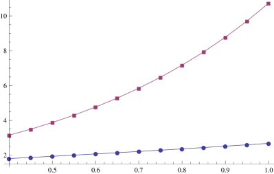
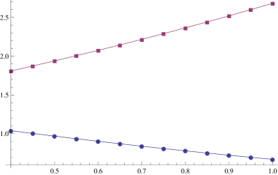
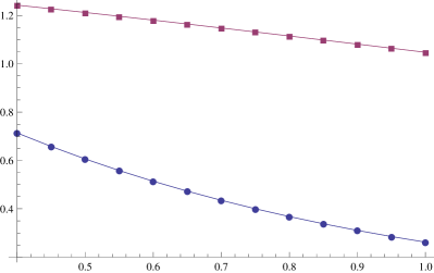
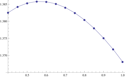
Figure 1: graphs of $\Lambda(s,m_{1},(0,L))$ (dots) and $\Lambda(s,m_{2},(0,L))$ (squares) as functions of $s\in[0.4,1]$, for $L=2.5$ (top left), $L=5$ (top right), $L=8$ (bottom left). At bottom right, the graph of $\Lambda(s,m_{1},(0,L))$ for $L=3.5$.

As we mentioned in the introduction, a relevant question is the one of comparing the two eigenvalues

$$\begin{split}\lambda_{1}(m,\Omega)&=\inf\left\{\int_{\mathcal{C}}|\nabla v(x,y)|^{2}dxdy:\int_{\Omega}m(x)v^{2}(x,0)dx=1,\int_{\Omega}m(x)v(x,0)dx=0\right\},\\ \overline{\mu}_{1}(m,\Omega)&=\inf\left\{\int_{\Omega}|\nabla u(x)|^{2}dx:\int_{\Omega}m(x)u^{2}(x)dx=1,\int_{\Omega}m(x)u(x)dx=0\right\},\end{split}$$

which correspond to the linearized version of (1.7) and (1.8), respectively. We conclude this section showing some simple numerical results in dimension $N=1$. Using the usual Fourier representation with basis defined in (1.2), we have that

$$\begin{split}mu&=\sum_{i}\left[\int_{\Omega}m(x)\left(\sum_{j}u_{j}\phi_{j}(x)\right)\phi_{i}(x)dx\right]\phi_{i}\\ &=\sum_{i}\left[\sum_{j}u_{j}\left(\int_{\Omega}m(x)\phi_{j}(x)\phi_{i}(x)dx\right)\right]\phi_{i}:=\sum_{i}\left[\sum_{j}M_{ij}u_{j}\right]\phi_{i}.\end{split}$$

Under this point of view, solving the above minimization problems amounts to finding the smallest positive eigenvalue $\Lambda(s,m,\Omega)$ of the problem

$$\mathrm{diag}\left(\mu_{i}^{s}\right)_{i\geq 0}\mathbf{u}=\Lambda M\mathbf{u},$$

indeed $\lambda_{1}(m,\Omega)=\Lambda(1/2,m,\Omega)$ and $\overline{\mu}_{1}(m,\Omega)=\Lambda(1,m,\Omega)$. In turn, such eigenvalue can be easily approximated by truncating the Fourier series. In Figure 1 we report these approximations in the cases $\Omega=(0,L)$ and

$$m_{1}(x)=\cos\left(\frac{\pi}{L}x\right)-\frac{1}{2},\qquad m_{2}(x)=\cos\left(\frac{2\pi}{L}x\right)-\frac{1}{2}.$$

Hence $m$ has always mean equal to $1/2$, while

$$\mu_{1}(L)=\frac{\pi^{2}}{L^{2}}.$$

We observe that in the case $L=2.5<\pi$ then $\mu_{1}>1$, and thus $\Lambda$ is increasing in $s$ for any choice of $m$ as one can trivially prove. On the other hand, when $\mu_{1}<1$ the situation is more variegated. In any case, the eigenvalue corresponding to $m_{1}$ is always lower than the one corresponding to $m_{2}$, in agreement with the results obtained for similar weights in the case of the standard Laplacian in [10].

Eugenio Montefusco,
Dipartimento di Matematica,
Sapienza Università di Roma,
p.le Aldo Moro 5, 00185 Roma, Italy.
E-mail address: montefusco@mat.uniroma1.it

Benedetta Pellacci,
Dipartimento di Scienze Applicate,
Università degli Studi di Napoli Parthenope,
Centro Direzionale Isola C4, 80143 Napoli, Italy.
E-mail address: pellacci@uniparthenope.it

Gianmaria Verzini
Dipartimento di Matematica,
Politecnico di Milano,
p.za Leonardo da Vinci 32, 20133 Milano, Italy.
E-mail address: gianmaria.verzini@polimi.it

References

- [1] G. Alberti, G. Bouchitté, and P. Seppecher. Phase transition with the line-tension effect. Arch. Rational Mech. Anal., 144(1):1–46, 1998.
- [2] A. Ambrosetti and G. Prodi. A primer of nonlinear analysis, volume 34 of Cambridge Studies in Advanced Mathematics. Cambridge University Press, Cambridge, 1995. Corrected reprint of the 1993 original.
- [3] F. Andreu, J. M. Mazón, J. D. Rossi, and J. Toledo. The Neumann problem for nonlocal nonlinear diffusion equations. J. Evol. Equ., 8(1):189–215, 2008.
- [4] D. Applebaum. Lévy processes—from probability to finance and quantum groups. Notices Amer. Math. Soc., 51(11):1336–1347, 2004.
- [5] H. Berestycki, J.-M. Roquejoffre, and L. Rossi. The periodic patch model for population dynamics with fractional diffusion. Discrete Contin. Dyn. Syst. Ser. S, 4(1):1–13, 2011.
- [6] X. Cabré and J.-M. Roquejoffre. Propagation de fronts dans les équations de Fisher-KPP avec diffusion fractionnaire. C. R. Math. Acad. Sci. Paris, 347(23-24):1361–1366, 2009.
- [7] X. Cabré and J. Tan. Positive solutions of nonlinear problems involving the square root of the Laplacian. Adv. Math., 224(5):2052–2093, 2010.
- [8] L. Caffarelli and L. Silvestre. An extension problem related to the fractional Laplacian. Comm. Partial Differential Equations, 32(7-9):1245–1260, 2007.
- [9] L. A. Caffarelli, S. Salsa, and L. Silvestre. Regularity estimates for the solution and the free boundary of the obstacle problem for the fractional Laplacian. Invent. Math., 171(2):425–461, 2008.
- [10] R. S. Cantrell and C. Cosner. The effects of spatial heterogeneity in population dynamics. J. Math. Biol., 29(4):315–338, 1991.
- [11] R. S. Cantrell and C. Cosner. Conditional persistence in logistic models via nonlinear diffusion. Proc. Roy. Soc. Edinburgh Sect. A, 132(2):267–281, 2002.
- [12] A. Capella, J. Dávila, L. Dupaigne, and Y. Sire. Regularity of radial extremal solutions for some non-local semilinear equations. Comm. Partial Differential Equations, 36(8):1353–1384, 2011.
- [13] R. Cont and P. Tankov. Financial modelling with jump processes. Chapman & Hall/CRC Financial Mathematics Series. Chapman & Hall/CRC, Boca Raton, FL, 2004.
- [14] G. K. Gächter and M. J. Grote. Dirichlet-to-Neumann map for three-dimensional elastic waves. Wave Motion, 37(3):293–311, 2003.
- [15] Q.-Y. Guan and Z.-M. Ma. Reflected symmetric -stable processes and regional fractional Laplacian. Probab. Theory Related Fields, 134(4):649–694, 2006.
- [16] P. Hess. Periodic-parabolic boundary value problems and positivity, volume 247 of Pitman Research Notes in Mathematics Series. Longman Scientific & Technical, Harlow, 1991.
- [17] N. E. Humphries et al. Environmental context explains Levy and Brownian movement patterns of marine predators. Nature, 465(7301):1066–1069, 2010.
- [18] G. F. Madeira and A. S. do Nascimento. Bifurcation of stable equilibria and nonlinear flux boundary condition with indefinite weight. J. Differential Equations, 251(11):3228–3247, 2011.
- [19] A. Manes and A. M. Micheletti. Un’estensione della teoria variazionale classica degli autovalori per operatori ellittici del secondo ordine. Boll. Un. Mat. Ital. (4), 7:285–301, 1973.
- [20] R. Metzler and J. Klafter. The random walk’s guide to anomalous diffusion: a fractional dynamics approach. Phys. Rep., 339(1):77, 2000.
- [21] D. P. Nicholls and M. Taber. Joint analyticity and analytic continuation of Dirichlet-Neumann operators on doubly perturbed domains. J. Math. Fluid Mech., 10(2):238–271, 2008.
- [22] P. H. Rabinowitz. Some global results for nonlinear eigenvalue problems. J. Functional Analysis, 7:487–513, 1971.
- [23] A. M. Reynolds and C. J. Rhodes. The Lévy flight paradigm: random search patterns and mechanisms. Ecology, 90(4):877–887, 2009.
- [24] O. Savin and E. Valdinoci. Elliptic PDEs with fibered nonlinearities. J. Geom. Anal., 19(2):420–432, 2009.
- [25] M. Shlesinger, G. Zaslavsky, and J. Klafter. Strange Kinetics. Nature, 363(6424):31–37, 1993.
- [26] J. G. Skellam. Random dispersal in theoretical populations. Biometrika, 38:196–218, 1951.
- [27] G. M. Troianiello. Elliptic differential equations and obstacle problems. The University Series in Mathematics. Plenum Press, New York, 1987.
- [28] K. Umezu. Behavior and stability of positive solutions of nonlinear elliptic boundary value problems arising in population dynamics. Nonlinear Anal., 49(6, Ser. A: Theory Methods):817–840, 2002.
- [29] G. Viswanathan et al. Levy flight search patterns of wandering albatrosses. Nature, 381(6581):413–415, 1996.