A finite volume scheme for a Keller-Segel model
with additional cross-diffusion

Abstract.

A finite volume scheme for the (Patlak-) Keller-Segel model in two space dimensions with an additional cross-diffusion term in the elliptic equation for the chemical signal is analyzed. The main feature of the model is that there exists a new entropy functional yielding gradient estimates for the cell density and chemical concentration. The main features of the numerical scheme are positivity preservation, mass conservation, entropy stability, and—under additional assumptions—entropy dissipation. The existence of a discrete solution and its numerical convergence to the continuous solution is proved. Furthermore, temporal decay rates for convergence of the discrete solution to the homogeneous steady state is shown using a new discrete logarithmic Sobolev inequality. Numerical examples point out that the solutions exhibit intermediate states and that there exist nonhomogeneous stationary solutions with a finite cell density peak at the domain boundary.

1. Introduction

Chemotaxis, the directed movement of cells in response to chemical gradients, plays an important role in many biological fields, such as embryogenesis, immunology, cancer growth, and wound healing [21, 31]. At the macroscopic level, chemotaxis models can be formulated in terms of the cell density $n(x,t)$ and the concentration of the chemical signal $S(x,t)$. A classical model to describe the time evolution of these two variables is the (Patlak-) Keller-Segel system, suggested by Patlak in 1953 [29] and Keller and Segel in 1970 [24]. Assuming that the time scale of the chemical signal is much larger than that of the cell movement, the classical parabolic-elliptic Keller-Segel equations read as follows:

$$\partial_{t}n=\operatorname{div}(\nabla n-n\nabla S),\quad 0=\Delta S+\mu n-S\quad\mbox{in }\Omega,$$

where $\Omega\subset{\mathbb{R}}^{2}$ is a bounded domain or $\Omega={\mathbb{R}}^{2}$, with homogeneous Neumann boundary and initial conditions. The parameter $\mu>0$ is the secretion rate at which the chemical substance is emitted by the cells. The nonlinear term $n\nabla S$ models the cell movement towards higher concentrations of the chemical signal.

This model exhibits the phenomenon of cell aggregation. The more cells are aggregated, the more the attracting chemical signal is produced by the cells. This process is counterbalanced by cell diffusion, but if the cell density is sufficiently large, the nonlocal chemical interaction dominates diffusion and results in a blow-up of the cell density. In two space dimensions, the critical threshold for blow-up is given by $M=\int_{\Omega}n_{0}dx=4\pi$ if $\Omega$ is a bounded connected domain with $C^{2}$ boundary [27] and $M=8\pi$ in the radial and whole-space case [3, 28]. The existence and uniqueness of smooth global-in-time solutions in the subcritical case is proved for bounded domains in [23] and in the whole space in [5]. In the critical case $M=8\pi$, a global whole-space solution exists, which becomes unbounded as $t\to\infty$ [4]. Furthermore, there exist radially symmetric initial data such that, in the supercritical case, the solution forms a $\delta$-singularity in finite time [20].

Motivated by numerical and modeling issues, the question how blow up can be avoided has been investigated intensively the last years. It has been suggested to modify the chemotactic sensitivity (modeling, e.g., volume-filling effects), to allow for degenerate cell diffusion, or to include suitable growth-death terms. We refer to [22] for references. Another idea is to introduce additional cell diffusion in the equation for the chemical concentration [9, 22]. This diffusion term avoids, even for arbitrarily small diffusion constants, the blow-up and leads to the global-in-time existence of weak solutions [22]. The model, which is investigated in this paper, reads as follows:

(1) $$\partial_{t}n=\operatorname{div}(\nabla n-n\nabla S),\quad 0=\Delta S+\delta\Delta n+\mu n-S,\quad x\in\Omega,\ t>0,$$

where $\delta>0$ is the additional diffusion constant. We impose the homogeneous Neumann boundary and initial conditions

(2) $$\nabla n\cdot\nu=\nabla S\cdot\nu=0\quad\mbox{on }\partial\Omega,\ t>0,\quad n(\cdot,0)=n_{0}\quad\mbox{in }\Omega.$$

The advantage of the additional diffusion term is that blow-up of solutions is translated to large gradients which may help to determine the blow-up time numerically. Another advantage is that the enlarged system (1) exhibits an interesting entropy structure (see below).

At first sight, the additional term $\delta\Delta n$ seems to complicate the mathematical analysis. Indeed, the resulting diffusion matrix of the system is neither symmetric nor positive definite, and we cannot apply the maximum principle to the equation for the chemical signal anymore. It was shown in [22] that all these difficulties can be resolved by the observation that the above system possesses a logarithmic entropy,

$$E(t)=\int_{\Omega}\big{(}n(\log n-1)+1\big{)}dx,$$

which is dissipated according to

(3) $$\frac{dE}{dt}+\int_{\Omega}\left(4|\nabla\sqrt{n}|^{2}+\frac{1}{\delta}|\nabla S|^{2}+\frac{1}{\delta}S^{2}\right)dx=\frac{\mu}{\delta}\int_{\Omega}nSdx.$$

Suitable Gagliardo-Nirenberg inequalities applied to the right-hand side lead to gradient estimates for $\sqrt{n}$ and $S$, which are the starting point for the global existence and long-time analysis.

In this paper, we aim at developing a finite volume scheme which preserves the entropy structure on the discrete level by generalizing the scheme proposed in [16]. In contrast to [16], we are able to prove the existence of discrete solutions and their numerical convergence to the continuous solution for all values of the initial mass. Moreover, we show that the discrete solution converges for large times to the homogeneous steady state if $\mu$ or $1/\delta$ are sufficiently small, using a new discrete logarithmic Sobolev inequality (Proposition 3).

In the literature, there exist several approaches to solve the classical Keller-Segel system numerically. The parabolic-elliptic model was approximated by using finite difference [34, 36] or finite element methods [25, 32, 35]. Also a dynamic moving-mesh method [6], a variational steepest descent approximation scheme [2], and a stochastic particle approximation [18, 19] were developed. Concerning numerical schemes for the parabolic-parabolic model (in which $\partial_{t}S$ is added to the second equation in (1)), we mention the second-order central-upwind finite volume method of [11], the discontinuous finite element approach of [14], and the conservative finite element scheme of [33]. We also cite the paper [7] for a mixed finite element discretization of a Keller-Segel model with nonlinear diffusion.

There are only a few works in which a numerical analysis of the scheme was performed. Filbet proved the existence and numerical convergence of finite volume solutions [16]. Error estimates for a conservative finite element approximation were shown by Saito [32, 33]. Epshteyn and Izmirlioglu proved error estimates for a fully discrete discontinuous finite element method [14]. Convergence proofs for other schemes can be found in, e.g., [2, 19].

This paper contains the first numerical analysis for the Keller-Segel model (1) with additional cross-diffusion. Its originality comes from the fact that we “translate” all the analytical properties of [22] on a discrete level, namely positivity preservation, mass conservation, entropy stability, and entropy dissipation (under additional hypotheses).

The paper is organized as follows. Section 2 is devoted to the description of the finite volume scheme and the formulation of the main results. The existence of a discrete solution is shown in Section 3. A discrete version of the entropy-dissipation relation (3) and corresponding gradient estimates are proved in Section 4. These estimates allow us to obtain in Section 5 the convergence of the discrete solution to the continuous one when the approximation parameters tend to zero. A proof of the discrete logarithmic Sobolev inequality is given in Section 6. The long-time behavior of the discrete solution is investigated in Section 7. Finally, we present some numerical examples in Section 8 and compare the discrete solutions to our model (1) with those computed from the classical Keller-Segel system.

2. Numerical scheme and main results

In this section, we introduce the finite volume scheme and present our main results.

2.1. Notations and assumptions

Let $\Omega\subset{\mathbb{R}}^{2}$ be an open, bounded, polygonal subset. An admissible mesh of $\Omega$ is given by a family $\mathcal{T}$ of control volumes (open and convex polygons), a family $\mathcal{E}$ of edges, and a family of points $(x_{K})_{K\in\mathcal{T}}$ which satisfy Definition 9.1 in [15]. This definition implies that the straight line between two neighboring centers of cells $(x_{K},x_{L})$ is orthogonal to the edge $\sigma=K|L$. For instance, Voronoi meshes are admissible meshes [15, Example 9.2]. Triangular meshes satisfy the admissibility condition if all angles of the triangles are smaller than $\pi/2$ [15, Example 9.1].

We distinguish the interior edges $\sigma\in\mathcal{E}_{\rm int}$ and the boundary edges $\sigma\in\mathcal{E}_{\rm ext}$. The set of edges $\mathcal{E}$ equals the union $\mathcal{E}_{\rm int}\cup\mathcal{E}_{\rm ext}$. For a control volume $K\in\mathcal{T}$, we denote by $\mathcal{E}_{K}$ the set of its edges, by $\mathcal{E}_{{\rm int},K}$ the set of its interior edges, and by $\mathcal{E}_{{\rm ext},K}$ the set of edges of $K$ included in $\partial\Omega$.

Furthermore, we denote by d the distance in ${\mathbb{R}}^{2}$ and by m the Lebesgue measure in ${\mathbb{R}}^{2}$ or ${\mathbb{R}}$. We assume that the family of meshes satisfies the following regularity requirement: there exists $\xi>0$ such that for all $K\in\mathcal{T}$ and all $\sigma\in\mathcal{E}_{{\rm int},K}$ with $\sigma=K|L$, it holds

(4) $$\text{\rm d}(x_{K},\sigma)\geq\xi\,\text{\rm d}(x_{K},x_{L}).$$

This hypothesis is needed to apply discrete Sobolev-type inequalities [1]. Introducing for $\sigma\in\mathcal{E}$ the notation

$$d_{\sigma}=\left\{\begin{array}[]{ll}\text{\rm d}(x_{K},x_{L})&\quad\mbox{if }\sigma\in\mathcal{E}_{\rm int},\ \sigma=K|L,\\ \text{\rm d}(x_{K},\sigma)&\quad\mbox{if }\sigma\in\mathcal{E}_{{\rm ext},K},\end{array}\right.$$

we define the transmissibility coefficient

$$\tau_{\sigma}=\frac{\text{\rm m}(\sigma)}{d_{\sigma}},\quad\sigma\in\mathcal{E}.$$

The size of the mesh is denoted by

$$\Delta x=\max_{K\in\mathcal{T}}\text{diam}(K).$$

Let $T>0$ be some final time and $M_{T}$ the number of time steps. Then the time step size and the time points are given by, respectively,

$$\Delta t=\frac{T}{M_{T}},\quad t^{k}=k\Delta t,\quad 0\leq k\leq M_{T}.$$

We denote by $\mathcal{D}$ an admissible space-time discretization of $\Omega_{T}=\Omega\times(0,T)$ composed of an admissible mesh $\mathcal{T}$ of $\Omega$ and the values $\Delta t$ and $M_{T}$. The size of this space-time discretization $\mathcal{D}$ is defined by $\eta=\max\{\Delta x,\Delta t\}$.

Let $X(\mathcal{T})$ be the linear space of functions $\Omega\to{\mathbb{R}}$ which are constant on each cell $K\in\mathcal{T}$. We define on $X(\mathcal{T})$ the discrete $L^{p}$ norm, discrete $W^{1,p}$ seminorm, and discrete $W^{1,p}$ norm by, respectively,

$$\|u\|_{0,p,\mathcal{T}} =\left(\sum_{K\in\mathcal{T}}\text{\rm m}(K)|u|^{p}\right)^{1/p},$$

$$|u|_{1,p,\mathcal{T}} =\left(\sum_{\sigma\in\mathcal{E}_{\rm int}}\frac{\text{\rm m}(\sigma)}{d_{\sigma}^{p-1}}|D_{\sigma}u|^{p}\right)^{1/p},$$

$$\|u\|_{1,p,\mathcal{T}} =\|u\|_{0,p,\mathcal{T}}+|u|_{1,p,\mathcal{T}},$$

where $u\in X(\mathcal{T})$, $1\leq p<\infty$, and $D_{\sigma}u=|u_{K}-u_{L}|$ for $\sigma=K|L\in\mathcal{E}_{\rm int}$.

2.2. Finite volume scheme and main results

We are now in the position to define the finite volume discretization of (1)-(2). Let $\mathcal{D}$ be a finite volume discretization of $\Omega_{T}$. The initial datum $n_{0}$ is approximated by its $L^{2}$ projection on control volumes:

(5) $$n^{0}_{\mathcal{D}}=\sum_{K\in\mathcal{T}}n_{K}^{0}\mathbf{1}_{K},\quad\mbox{where }n^{0}_{K}=\frac{1}{\text{\rm m}(K)}\int_{K}n_{0}(x)dx,$$

and $\mathbf{1}_{K}$ is the characteristic function on $K$. Denoting by $n^{k}_{K}$ and $S^{k}_{K}$ approximations of the mean value of $n(\cdot,t^{k})$ and $S(\cdot,t^{k})$ on $K$, respectively, the numerical scheme reads as follows:

(6) $$\text{\rm m}(K)\frac{n^{k+1}_{K}-n^{k}_{K}}{\Delta t}-\sum_{\sigma\in\mathcal{E}_{K}}\tau_{\sigma}Dn_{K,\sigma}^{k+1}+\sum_{\begin{subarray}{c}\sigma\in\mathcal{E}_{\rm int},\\ \sigma=K|L\end{subarray}}\tau_{\sigma}\big{(}(DS^{k+1}_{K,\sigma})^{+}n_{K}^{k+1}-(DS^{k+1}_{K,\sigma})^{-}n_{L}^{k+1}\big{)}=0,$$

(7) $$-\sum_{\sigma\in\mathcal{E}_{K}}\tau_{\sigma}DS^{k+1}_{K,\sigma}-\delta\sum_{\sigma\in\mathcal{E}_{K}}\tau_{\sigma}Dn^{k+1}_{K,\sigma}=\text{\rm m}(K)(\mu n_{K}^{k+1}-S_{K}^{k+1}),$$

for all $K\in\mathcal{T}$ and $0\leq k\leq M_{T}-1$. Here, $v^{+}=\max\{0,v\}$, $v^{-}=\max\{0,-v\}$, and

(8) $$DU_{K,\sigma}^{k}=\left\{\begin{array}[]{ll}U_{L}^{k}-U_{K}^{k}&\quad\mbox{for }\sigma=K|L\in\mathcal{E}_{{\rm int},K},\\ 0&\quad\mbox{for }\sigma\in\mathcal{E}_{{\rm ext},K}.\end{array}\right.$$

The approximation $S^{0}_{K}$ is computed from (7) with $k=-1$. This scheme is based on a fully implicit Euler discretization in time and a finite volume approach for the volume variable. The implicit scheme allows us to establish discrete entropy-dissipation estimates which would not be possible with an explicit scheme. This approximation is similar to that in [16] except the additional cross-diffusion term in the second equation.

The numerical approximations $n_{\mathcal{D}}$ and $S_{\mathcal{D}}$ of $n$ and $S$ are defined by

$$n_{\mathcal{D}}(x,t)=\sum_{K\in\mathcal{T}}n_{K}^{k+1}\mathbf{1}_{K}(x),\quad S_{\mathcal{D}}(x,t)=\sum_{K\in\mathcal{T}}S_{K}^{k+1}\mathbf{1}_{K}(x),\quad\mbox{where }x\in\Omega,\ t\in(t^{k},t^{k+1}],$$

and $k=0,\ldots,M_{T}-1$. Furthermore, we define approximations $\nabla^{\mathcal{D}}n_{\mathcal{D}}$ and $\nabla^{\mathcal{D}}S_{\mathcal{D}}$ of the gradients of $n$ and $S$, respectively. To this end, we introduce a dual mesh: for $K\in\mathcal{T}$ and $\sigma\in\mathcal{E}_{K}$, let $T_{K,\sigma}$ be defined by:

• If $\sigma=K|L\in\mathcal{E}_{{\rm int},K}$, $T_{K,\sigma}$ is the cell (“diamond”) whose vertices are given by $x_{K}$, $x_{L}$, and the end points of the edge $\sigma=K|L$.

• If $\sigma\in\mathcal{E}_{{\rm ext},K}$, $T_{K,\sigma}$ is the cell (“triangle”) whose vertices are given by $x_{K}$ and the end points of the edge $\sigma=K|L$.

An example of construction of $T_{K,\sigma}$ can be found in [10]. Clearly, $T_{K,\sigma}$ defines a partition of $\Omega$. The approximate gradient $\nabla^{\mathcal{D}}n_{\mathcal{D}}$ is a piecewise constant function, defined in $\Omega_{T}=\Omega\times(0,T)$ by

$$\nabla^{\mathcal{D}}n_{\mathcal{D}}(x,t)=\frac{\text{\rm m}(\sigma)}{\text{\rm m}(T_{K,\sigma})}Dn_{K,\sigma}^{k+1}\nu_{K,\sigma},\quad x\in T_{K,\sigma},\ t\in(t^{k},t^{k+1}),$$

where $Dn_{K,\sigma}^{k+1}$ is given as in (8) and $\nu_{K,\sigma}$ is the unit vector normal to $\sigma$ and outward to $K$. The approximate gradient $\nabla^{\mathcal{D}}S_{\mathcal{D}}$ is defined in a similar way.

Our first result is the existence of solutions to the finite volume scheme.

Theorem 1 (Existence of finite volume solutions).

Let $\Omega\subset{\mathbb{R}}^{2}$ be an open, bounded, polygonal subset and let $\mathcal{D}$ be an admissible discretization of $\Omega\times(0,T)$. The initial datum satisfies $n_{0}\in L^{2}(\Omega)$, $n_{0}\geq 0$ in $\Omega$. Then there exists a solution $\{(n_{K}^{k},S_{K}^{k}),\,K\in\mathcal{T},\,0\leq k\leq M_{T}\}$ to (5)-(7) satisfying

(9) $$n_{K}^{k}\geq 0\quad\mbox{for all }K\in\mathcal{T},\,k\geq 0,$$

(10) $$\sum_{K\in\mathcal{T}}\text{\rm m}(K)n_{K}^{k}=\sum_{K\in\mathcal{T}}\text{\rm m}(K)n_{K}^{0}=\|n_{0}\|_{L^{1}(\Omega)}\quad\mbox{for all }k\geq 0.$$

Properties (9) and (10) show that the scheme is positivity preserving and mass conserving. It is also entropy stable; see (17) below.

Let $(\mathcal{D}_{\eta})_{\eta>0}$ be a sequence of admissible space-time discretizations indexed by the size $\eta=\max\{\Delta x,\Delta t\}$ of the discretization. We denote by $(\mathcal{T}_{\eta})_{\eta>0}$ the corresponding meshes of $\Omega$. We suppose that these discretizations satisfy (4) uniformly in $\eta$, i.e., $\xi>0$ does not depend on $\eta$. Let $(n_{\eta},S_{\eta}):=(n_{\mathcal{D}_{\eta}},S_{\mathcal{D}_{\eta}})$ be a finite volume solution, constructed in Theorem 1, on the discretization $\mathcal{D}_{\eta}$. We set $\nabla^{\eta}:=\nabla^{\mathcal{D}_{\eta}}$. Our second result concerns the convergence of $(n_{\eta},S_{\eta})$ to a weak solution $(n,S)$ to (1)-(2).

Theorem 2 (Convergence of the finite volume solutions).

Let the assumptions of Theorem 1 hold. Furthermore, let $(\mathcal{D}_{\eta})_{\eta>0}$ be a sequence of admissible discretizations satisfying (4) uniformly in $\eta$, and let $(n_{\eta},S_{\eta})$ be a sequence of finite volume solutions to (5)-(7). Then there exists $(n,S)$ such that, up to a subsequence,

$$n_{\eta}\to n \quad\mbox{strongly in }L^{2}(\Omega_{T}),$$

$$\nabla^{\eta}n_{\eta}\rightharpoonup\nabla n \quad\mbox{weakly in }L^{2}(\Omega_{T}),$$

$$S_{\eta}\rightharpoonup S,\ \nabla^{\eta}S_{\eta}\rightharpoonup\nabla S \quad\mbox{weakly in }L^{2}(\Omega_{T}),$$

and $(n,S)\in L^{2}(0,T;H^{1}(\Omega))^{2}$ is a weak solution to (1)-(2) in the sense of

(11) $$\int_{0}^{T}\int_{\Omega}(n\partial_{t}\phi-\nabla n\cdot\nabla\phi+n\nabla S\cdot\nabla\phi)dx+\int_{\Omega}n_{0}\phi(\cdot,0)dx =0,$$

(12) $$\int_{0}^{T}\int_{\Omega}(-\nabla S\cdot\nabla\phi-\delta\nabla n\cdot\nabla\phi+\mu n\phi-S\phi)dx =0$$

for all test functions $\phi\in C_{0}^{\infty}(\Omega\times[0,T])$.

It is shown in [22, Theorem 1.3] that, if the secretion rate $\mu>0$ is sufficiently small or the diffusion parameter $\delta>0$ is sufficiently large, the solution $(n,S)$ to (1)-(2) converges exponentially fast to the homogeneous steady state $(n^{*},S^{*})$, where $n^{*}=\|n_{0}\|_{L^{1}(\Omega)}/\text{\rm m}(\Omega)$ and $S^{*}=\mu n^{*}$. The proof in [22] is based on the logarithmic Sobolev inequality. Therefore, we state first a novel discrete version of this inequality, which is proved in Section 6.

Proposition 3 (Discrete logarithmic Sobolev inequality).

Let $\Omega\subset{\mathbb{R}}^{d}$ $(d\geq 1)$ be an open bounded polyhedral domain and let $\mathcal{T}$ be an admissible mesh of $\Omega$ satisfying (4). Then there exists a constant $C_{L}>0$ only depending on $\Omega$, $d$, and $\xi$ such that for all $u\in X(\mathcal{T})$,

$$\int_{\Omega}u^{2}\log\frac{u^{2}}{m^{-1}\|u\|_{0,2,\mathcal{T}}^{2}}dx\leq C_{L}|u|_{1,2,\mathcal{T}}^{2},$$

where we abbreviated $m=\text{\rm m}(\Omega)$.

The constant $C_{L}>0$ can be made more precise. Let $C_{S}(q)>0$ be the constant in the discrete Sobolev inequality [1, Theorem 4]

(13) $$\|u\|_{0,q,\mathcal{T}}\leq\frac{C_{S}(q)}{\sqrt{\xi}}\|u\|_{1,2,\mathcal{T}}\quad\mbox{for }u\in X(\mathcal{T}),$$

where $1\leq q\leq 2d/(d-2)$ (and $1\leq q<\infty$ if $d\leq 2$), and let $C_{P}(r)>0$ be the constant in the discrete Poincaré-Wirtinger inequality [1, Prop. 1]

(14) $$\|u-\bar{u}\|_{0,r,\mathcal{T}}\leq\frac{C_{P}(r)}{\sqrt{\xi}}|u|_{1,2,\mathcal{T}}\quad\mbox{for }u\in X(\mathcal{T}),$$

where $1\leq r\leq 2$ and $\bar{u}=m^{-1}\int_{\Omega}u(x)dx$, $m=\text{\rm m}(\Omega)$. Then

$$C_{L}=\frac{q}{(q-2)\xi}\left(C_{S}(q)^{2}+\frac{C_{S}(q)^{2}C_{P}(2)^{2}}{\xi}+\frac{q-4}{q}C_{P}(2)^{2}\right).$$

For our result on the long-time behavior, we introduce the discrete relative entropy

$$E[n^{k}|n^{*}]=\sum_{K\in\mathcal{T}}\text{\rm m}(K)n_{K}^{k}\log\left(\frac{n_{K}^{k}}{n^{*}}\right)\geq 0,\quad k\geq 0.$$

Theorem 4 (Long-time behavior of finite volume solutions).

Let the assumptions of Theorem 1 hold and let $(n_{\mathcal{D}},S_{\mathcal{D}})$ be a solution to (5)-(7). Then for all $k\geq 0$,

$$E[n^{k+1}|n^{*}]+\Delta t(1-C^{*})\big{|}\sqrt{n^{k+1}}\big{|}_{1,2,\mathcal{T}}^{2}+\frac{\Delta t}{2\delta}\|S^{k+1}-S^{*}\|_{1,2,\mathcal{T}}^{2}\leq E[n^{k}|n^{*}],$$

where $C^{*}=\mu^{2}C(\Omega)^{2}\|n_{0}\|_{L^{1}(\Omega)}/(\delta\xi)$, $C(\Omega)>0$ only depending on $\Omega$, and $\xi$ is the parameter in (4). In particular, if $C^{*}<1$, the discrete relative entropy is nonincreasing and

$$\|n^{k}-n^{*}\|_{0,1,\mathcal{T}} \leq\sqrt{4E[n^{0}|n^{*}]\|n_{0}\|_{L^{1}(\Omega)}}\left(1+\frac{1-C^{*}}{C_{L}}\Delta t\right)^{-k/2},$$

$$\|S^{k}-S^{*}\|_{1,2,\mathcal{T}} \leq\sqrt{\frac{2\delta E[n^{0}|n^{*}]}{\Delta t}}\left(1+\frac{1-C^{*}}{C_{L}}\Delta t\right)^{-(k-1)/2},\quad k\in{\mathbb{N}},$$

where $C_{L}>0$ is the constant in the discrete logarithmic Sobolev inequality (see Proposition 3). In particular, for each $K\in\mathcal{T}$,

$$(n_{K}^{k},S_{K}^{k})\to(n^{*},S^{*})\quad\mbox{as }k\to\infty.$$

In [22], the long-time behavior of solutions is shown under the condition $\mu^{2}\|n_{0}\|_{L^{1}(\Omega)}/\delta<C(\Omega)$ for a constant $C(\Omega)>0$ appearing in some Poincaré-Sobolev inequality. We observe that our condition depends additionally on the regularity of the finite volume mesh. The convergence of $\|n^{k}-n^{*}\|_{0,1,\mathcal{T}}$ is approximately exponential for sufficiently small $\Delta t>0$. The convergence result for $\|S^{k}-S^{*}\|_{1,2,\mathcal{T}}$ is weaker in view of the factor $(\Delta t)^{-1}$. In [22], the exponential convergence of $S-S^{*}$ is shown in the $L^{2}(\Omega)$ norm only and therefore, our result is not surprising.

3. Existence of finite volume solutions

In this section, we prove Theorem 1. The proof is based on the Brouwer fixed-point theorem. Let $k\in\{1,\ldots,M_{T}-1\}$ and let $(n^{k},S^{k})$ be a solution to (6) and (7), with $k+1$ replaced by $k$, satisfying (9)-(10). We introduce the set

$$Z=\{u\in X(\mathcal{T}):u\geq 0\mbox{ in }\Omega,\ \|u\|_{L^{1}(\Omega)}\leq\|n_{0}\|_{L^{1}(\Omega)}\}.$$

The finite-dimensional space $Z$ is convex and compact. In the following, we define the fixed-point operator by solving a linearized problem. First, we construct $\widetilde{S}\in X(\mathcal{T})$ using the following scheme:

(15) $$-\sum_{\sigma\in\mathcal{E}_{K}}\tau_{\sigma}D\widetilde{S}_{K,\sigma}+\text{\rm m}(K)\widetilde{S}_{K}=\delta\sum_{\sigma\in\mathcal{E}_{K}}\tau_{\sigma}Dn_{K,\sigma}^{k}+\mu\text{\rm m}(K)n_{K}^{k},\quad K\in\mathcal{T}.$$

Second, we compute $\widetilde{n}\in X(\mathcal{T})$ using the scheme

(16) $$\frac{\text{\rm m}(K)}{\Delta t}(\widetilde{n}_{K}-n_{K}^{k})-\sum_{\sigma\in\mathcal{E}_{K}}\tau_{\sigma}D\widetilde{n}_{K,\sigma}+\sum_{\begin{subarray}{c}\sigma\in\mathcal{E}_{\rm int},\\ \sigma=K|L\end{subarray}}\tau_{\sigma}\big{(}(D\widetilde{S}_{K,\sigma})^{+}\widetilde{n}_{K}-(D\widetilde{S}_{K,\sigma})^{-}\widetilde{n}_{L}\big{)}=0.$$

Step 1: Existence and uniqueness for (15) and (16). The linear system (15) can be written as $A\widetilde{S}=b$, where $A$ is the matrix with the elements

$$A_{K,K}=\sum_{\sigma\in\mathcal{E}_{K}}\tau_{\sigma}+\text{\rm m}(K),\quad A_{K,L}=-\tau_{\sigma}\quad\mbox{ for }K,L\in\mathcal{T}\mbox{ with }\sigma=K|L\in\mathcal{E}_{{\rm int},K},$$

and $b$ is the vector with the elements

$$b_{K}=\delta\sum_{\sigma\in\mathcal{E}_{K}}\tau_{\sigma}Dn_{K,\sigma}^{k}+\mu\text{\rm m}(K)n_{K}^{k}.$$

Since for all $L\in\mathcal{T}$,

$$|A_{L,L}|-\sum_{K\neq L}|A_{K,L}|=\text{\rm m}(L)>0,$$

the matrix $A$ is strictly diagonally dominant with respect to the columns and hence, $A$ is invertible. This shows the unique solvability of (15).

Similarly, (16) can be written as $B\widetilde{n}=c$, where $B$ is the matrix with the elements

$$B_{K,K} =\frac{\text{\rm m}(K)}{\Delta t}+\sum_{\sigma\in\mathcal{E}_{K}}\tau_{\sigma}(1+(D\widetilde{S}_{K,\sigma})^{+}),\quad K\in\mathcal{T},$$

$$B_{K,L} =-\tau_{\sigma}(1+(D\widetilde{S}_{K,\sigma})^{-}),\quad\mbox{ for }K,L\in\mathcal{T}\mbox{ with }\sigma=K|L\in\mathcal{E}_{{\rm int},K},$$

and $c$ is the vector with the elements $c_{K}=\text{\rm m}(K)n^{k}_{K}/\Delta t$, $K\in\mathcal{T}$. The diagonal elements of $B$ are positive, and the off-diagonal elements are nonpositive. Moreover, $B$ is strictly diagonal dominant with respect to the columns since for all $\sigma=K|L\in\mathcal{E}_{{\rm int},K}$, we have $D\widetilde{S}_{L,\sigma}=-D\widetilde{S}_{K,\sigma}$ which yields $(D\widetilde{S}_{L,\sigma})^{+}=(D\widetilde{S}_{K,\sigma})^{-}$ and hence,

$$|B_{L,L}|-\sum_{K\neq L}|B_{K,L}|=\frac{\text{\rm m}(L)}{\Delta t}>0.$$

We infer that $B$ is an M-matrix and invertible, which gives the existence and uniqueness of a solution $\widetilde{n}$ to (16).

The M-matrix property of $B$ implies that $B^{-1}$ is positive. As a consequence, since $n^{k}$ and $c$ are nonnegative componentwise, by the induction hypothesis, $\widetilde{n}=B^{-1}c$ is nonnegative componentwise. This means that $\widetilde{n}$ satisfies (9). Summing (16) over $K\in\mathcal{T}$, we compute

$$\sum_{K\in\mathcal{T}}\text{\rm m}(K)\widetilde{n}_{K}=\sum_{K\in\mathcal{T}}\text{\rm m}(K)n_{K}^{k}=\|n_{0}\|_{L^{1}(\Omega)}.$$

Step 2: Continuity of the fixed-point operator. The solution to (15) and (16) defines the fixed-point operator $F:Z\to Z$, $F(n)=\widetilde{n}$. We have to show that $F$ is continuous. For this, let $(n^{\gamma})_{\gamma\in{\mathbb{N}}}\subset Z$ be a sequence converging to $n$ in $X(\mathcal{T})$ as $\gamma\to\infty$. Setting $\widetilde{n}^{\gamma}=F(n^{\gamma})$ and $\widetilde{n}=F(n)$, we have to prove that $\widetilde{n}^{\gamma}\to\widetilde{n}$ in $X(\mathcal{T})$. Using the scheme (15), we construct first $\widetilde{S}^{\gamma}$ (respectively, $\widetilde{S}$) from $n^{\gamma}$ (respectively, $n$). Then, using the scheme (16), we obtain $\widetilde{n}^{\gamma}$ (respectively, $\widetilde{n}$).

We claim that $\widetilde{S}^{\gamma}-\widetilde{S}\to 0$ in $X(\mathcal{T})$ as $\gamma\to\infty$. Indeed, since the map $n\mapsto\tilde{S}$, where $\tilde{S}$ is constructed from (15), is linear on the finite dimensional space $X(\mathcal{T})$, it is obviously continuous. Moreover, using the scheme (16) and performing the same computations as in the proof of Theorem 2.1 in [16], it follows that

$$\sum_{K\in\mathcal{T}}\text{\rm m}(K)|\widetilde{n}^{\gamma}_{K}-\widetilde{n}_{K}|\leq 2\Delta t\bigg{(}\sum_{K\in\mathcal{T}}|\widetilde{n}_{K}|^{2}\bigg{)}^{1/2}\bigg{(}\sum_{K\in\mathcal{T}}\sum_{\sigma\in\mathcal{E}_{K}}\tau_{\sigma}|D(\widetilde{S}^{\gamma}-\widetilde{S})_{K,\sigma}|^{2}\bigg{)}^{1/2}.$$

The right-hand side converges to zero as $\widetilde{S}^{\gamma}\to\widetilde{S}$ in $X(\mathcal{T})$, which proves that $\widetilde{n}^{\gamma}\to\widetilde{n}$ in $X(\mathcal{T})$.

Step 3: Application of the fixed-point theorem. The assumptions of the Brouwer fixed-point theorem are satisfied, implying the existence of a fixed point of $F$, i.e. of a solution $n^{k+1}$ to (6) satisfying (9). We have shown in Step 1 that (10) holds for $n^{k+1}$. Finally, we construct $S^{k+1}$ using scheme (7).

4. A priori estimates

The proof of Theorem 2 is based on suitable a priori estimates which are shown in this section. We introduce a discrete version of the entropy functional used in [22]:

$$E^{k}=\sum_{K\in\mathcal{T}}\text{\rm m}(K)H(n_{K}^{k}),\quad\mbox{where }H(s)=s(\log s-1)+1.$$

Proposition 5 (Entropy stability).

There exists a constant $C>0$ only depending on $\Omega$, $\mu$, $\delta$, $\|n_{0}\|_{L^{1}(\Omega)}$, and $\xi$ (see (4)) such that for all $k\geq 0$,

$$E^{k+1}-E^{k} +\frac{\Delta t}{2}\sum_{\sigma\in\mathcal{E}_{\rm int}}\tau_{\sigma}\big{|}D(\sqrt{n^{k+1}})_{K,\sigma}\big{|}^{2}+\frac{\Delta t}{\delta}\sum_{K\in\mathcal{T}}\text{\rm m}(K)|S^{k+1}|^{2}$$

(17) $${}+\frac{\Delta t}{\delta}\sum_{\sigma\in\mathcal{E}_{\rm int}}\tau_{\sigma}|DS_{K,\sigma}^{k+1}|^{2}\leq C\Delta t.$$

Proof.

By the convexity of $H$, we find that

$$E^{k+1}-E^{k}=\sum_{K\in\mathcal{T}}\text{\rm m}(K)\big{(}H(n_{K}^{k+1})-H(n_{K}^{k})\big{)}\leq\sum_{K\in\mathcal{T}}\text{\rm m}(K)\log(n_{K}^{k+1})(n_{K}^{k+1}-n_{K}^{k}).$$

Inserting the scheme (6), we can write

$$E^{k+1}-E^{k} \leq\Delta t\sum_{\begin{subarray}{c}\sigma\in\mathcal{E}_{\rm int},\\ \sigma=K|L\end{subarray}}\tau_{\sigma}(n^{k+1}_{L}-n^{k+1}_{K})\log n_{K}^{k+1}$$

(18) $$\phantom{xx}{}-\Delta t\sum_{\begin{subarray}{c}\sigma\in\mathcal{E}_{\rm int},\\ \sigma=K|L\end{subarray}}\tau_{\sigma}\big{(}(DS^{k+1}_{K,\sigma})^{+}n_{K}^{k+1}-(DS^{k+1}_{K,\sigma})^{-}n_{L}^{k+1}\big{)}\log n_{K}^{k+1}=:I_{1}+I_{2}.$$

Now, we argue similarly as in the proof of Lemma 3.1 in [16]. We employ the symmetry of $\tau_{\sigma}$ and a Taylor expansion of $\log$ around $n_{K}^{k+1}$ to infer that

$$I_{1} =-\Delta t\sum_{\begin{subarray}{c}\sigma\in\mathcal{E}_{\rm int},\\ \sigma=K|L\end{subarray}}\tau_{\sigma}(n_{K}^{k+1}-n_{L}^{k+1})(\log n_{K}^{k+1}-\log n_{L}^{k+1})$$

$$=-\Delta t\sum_{\begin{subarray}{c}\sigma\in\mathcal{E}_{\rm int},\\ \sigma=K|L\end{subarray}}\tau_{\sigma}(n_{K}^{k+1}-n_{L}^{k+1})^{2}\frac{1}{\bar{n}_{\sigma}^{k+1}}=-\Delta t\sum_{\begin{subarray}{c}\sigma\in\mathcal{E}_{\rm int},\\ \sigma=K|L\end{subarray}}\tau_{\sigma}\left(\frac{Dn_{K,\sigma}^{k+1}}{\sqrt{\bar{n}_{\sigma}^{k+1}}}\right)^{2},$$

where $\bar{n}_{\sigma}^{k+1}=t_{\sigma}n_{K}^{k+1}+(1-t_{\sigma})n_{L}^{k+1}$ for some $t_{\sigma}\in(0,1)$. We perform a summation by parts in $I_{2}$, using again the symmetry of $\tau_{\sigma}$:

$$I_{2}=-\Delta t\sum_{\begin{subarray}{c}\sigma\in\mathcal{E}_{\rm int},\\ \sigma=K|L\end{subarray}}\tau_{\sigma}\big{(}(DS^{k+1}_{K,\sigma})^{+}n_{K}^{k+1}-(DS^{k+1}_{K,\sigma})^{-}n_{L}^{k+1}\big{)}(\log n_{K}^{k+1}-\log n_{L}^{k+1}).$$

Reordering the sum and using the expression for $\bar{n}_{\sigma}^{k+1}$ in the Taylor expansion of log, it is shown in [16, p. 468] that

$$I_{2}\leq-\Delta t\sum_{\begin{subarray}{c}\sigma\in\mathcal{E}_{\rm int},\\ \sigma=K|L\end{subarray}}\tau_{\sigma}\bar{n}_{\sigma}^{k+1}DS_{K,\sigma}^{k+1}(\log n_{K}^{k+1}-\log n_{L}^{k+1}).$$

The Taylor expansion shows that $\bar{n}_{\sigma}^{k+1}(\log n_{K}^{k+1}-\log n_{L}^{k+1})=n_{K}^{k+1}-n_{L}^{k+1}$, which gives

$$I_{2}\leq-\Delta t\sum_{\begin{subarray}{c}\sigma\in\mathcal{E}_{\rm int},\\ \sigma=K|L\end{subarray}}\tau_{\sigma}DS_{K,\sigma}^{k+1}(n_{K}^{k+1}-n_{L}^{k+1})=\Delta t\sum_{\begin{subarray}{c}\sigma\in\mathcal{E}_{\rm int},\\ \sigma=K|L\end{subarray}}\tau_{\sigma}DS_{K,\sigma}^{k+1}Dn_{K,\sigma}^{k+1}.$$

Summarizing the estimates for $I_{1}$ and $I_{2}$, (18) leads to

(19) $$E^{k+1}-E^{k}\leq-\Delta t\sum_{\begin{subarray}{c}\sigma\in\mathcal{E}_{\rm int},\\ \sigma=K|L\end{subarray}}\tau_{\sigma}\left(\frac{Dn_{K,\sigma}^{k+1}}{\sqrt{\bar{n}_{\sigma}^{k+1}}}\right)^{2}+\Delta t\sum_{\begin{subarray}{c}\sigma\in\mathcal{E}_{\rm int},\\ \sigma=K|L\end{subarray}}\tau_{\sigma}DS_{K,\sigma}^{k+1}Dn_{K,\sigma}^{k+1}.$$

The first term can be estimated for $\sigma=K|L$ as follows:

(20) $$\frac{|Dn_{K,\sigma}^{k+1}|}{\sqrt{\bar{n}_{\sigma}^{k+1}}}=\frac{\sqrt{n_{L}^{k+1}}+\sqrt{n_{K}^{k+1}}}{\sqrt{\bar{n}_{\sigma}^{k+1}}}|D(\sqrt{n^{k+1}})_{K,\sigma}|\geq|D(\sqrt{n^{k+1}})_{K,\sigma}|.$$

In order to bound the second term, we multiply the scheme (7) by $(\Delta t/\delta)S_{K}^{k+1}$ and sum over $K\in\mathcal{T}$:

$$0 =\frac{\Delta t}{\delta}\sum_{K\in\mathcal{T}}\sum_{\sigma\in\mathcal{E}_{K}}\tau_{\sigma}DS_{K,\sigma}^{k+1}S_{K}^{k+1}+\Delta t\sum_{K\in\mathcal{T}}\sum_{\sigma\in\mathcal{E}_{K}}\tau_{\sigma}Dn_{K,\sigma}^{k+1}S_{K}^{k+1}$$

$$\phantom{xx}{}+\frac{\mu\Delta t}{\delta}\sum_{K\in\mathcal{T}}\text{\rm m}(K)n_{K}^{k+1}S_{K}^{k+1}-\frac{\Delta t}{\delta}\sum_{K\in\mathcal{T}}\text{\rm m}(K)|S_{K}^{k+1}|^{2}.$$

By summation by parts, we find that

$$\Delta t\sum_{\begin{subarray}{c}\sigma\in\mathcal{E}_{\rm int},\\ \sigma=K|L\end{subarray}}\tau_{\sigma}Dn_{K,\sigma}^{k+1}DS_{K,\sigma}^{k+1} =-\frac{\Delta t}{\delta}\sum_{\begin{subarray}{c}\sigma\in\mathcal{E}_{\rm int},\\ \sigma=K|L\end{subarray}}\tau_{\sigma}|DS_{K,\sigma}^{k+1}|^{2}+\frac{\mu\Delta t}{\delta}\sum_{K\in\mathcal{T}}\text{\rm m}(K)n_{K}^{k+1}S_{K}^{k+1}$$

(21) $$\phantom{xx}{}-\frac{\Delta t}{\delta}\sum_{K\in\mathcal{T}}\text{\rm m}(K)|S_{K}^{k+1}|^{2}.$$

Inserting (21) into (19) and employing (20), it follows that

$$E^{k+1}-E^{k} +\Delta t\sum_{\begin{subarray}{c}\sigma\in\mathcal{E}_{\rm int},\\ \sigma=K|L\end{subarray}}\tau_{\sigma}|D(\sqrt{n^{k+1}})_{K,\sigma}|^{2}+\frac{\Delta t}{\delta}\sum_{K\in\mathcal{T}}\text{\rm m}(K)|S_{K}^{k+1}|^{2}$$

(22) $${}+\frac{\Delta t}{\delta}\sum_{\begin{subarray}{c}\sigma\in\mathcal{E}_{\rm int},\\ \sigma=K|L\end{subarray}}\tau_{\sigma}|DS_{K,\sigma}^{k+1}|^{2}\leq\frac{\mu\Delta t}{\delta}\sum_{K\in\mathcal{T}}\text{\rm m}(K)n_{K}^{k+1}S_{K}^{k+1}.$$

It remains to estimate the right-hand side. We follow the proof of Proposition 3.1 in [22]. The Hölder inequality yields

(23) $$\mu\sum_{K\in\mathcal{T}}\text{\rm m}(K)n_{K}^{k+1}S_{K}^{k+1}\leq\mu\|n^{k+1}\|_{0,6/5,\mathcal{T}}\|S^{k+1}\|_{0,6,\mathcal{T}}.$$

The discrete $L^{6}$ norm of $S^{k+1}$ can be bounded by the discrete $H^{1}$ norm using the discrete Sobolev inequality (13)

$$\|S^{k+1}\|_{0,6,\mathcal{T}}\leq C\|S^{k+1}\|_{1,2,\mathcal{T}},$$

where $C>0$ depends only on $\Omega$ and $\xi$. For the discrete $L^{6/5}$ norm of $n^{k+1}$, we employ the discrete Gagliardo-Nirenberg inequality [1, Theorem 3] with $\theta=1/6$:

$$\|n^{k+1}\|_{0,6/5,\mathcal{T}}=\big{\|}\sqrt{n^{k+1}}\big{\|}_{0,12/5,\mathcal{T}}^{2}\leq C\big{\|}\sqrt{n^{k+1}}\big{\|}_{0,2,\mathcal{T}}^{2(1-\theta)}\big{\|}\sqrt{n^{k+1}}\big{\|}_{1,2,\mathcal{T}}^{2\theta},$$

where $C>0$ depends only on $\Omega$ and $\xi$. Mass conservation (10) implies that

$$\|n^{k+1}\|_{0,6/5,\mathcal{T}}\leq C\|n_{0}\|_{L^{1}(\Omega)}^{1-\theta}\left(\|n_{0}\|_{L^{1}(\Omega)}^{1/2}+\big{|}\sqrt{n^{k+1}}\big{|}_{1,2,\mathcal{T}}\right)^{2\theta}.$$

With these estimates, (23) becomes

$$\mu\sum_{K\in\mathcal{T}}\text{\rm m}(K)n_{K}^{k+1}S_{K}^{k+1} \leq C\mu\|S^{k+1}\|_{1,2,\mathcal{T}}\|n_{0}\|_{L^{1}(\Omega)}^{1-\theta}\left(\|n_{0}\|_{L^{1}(\Omega)}^{1/2}+\big{|}\sqrt{n^{k+1}}\big{|}_{1,2,\mathcal{T}}\right)^{2\theta}$$

$$\leq 2C\mu\|S^{k+1}\|_{1,2,\mathcal{T}}\|n_{0}\|_{L^{1}(\Omega)}^{1-\theta}\left(\|n_{0}\|_{L^{1}(\Omega)}+\big{|}\sqrt{n^{k+1}}\big{|}_{1,2,\mathcal{T}}^{2}\right)^{\theta}.$$

Then, by Young’s inequality with $p_{1}=2$, $p_{2}=2/(1-2\theta)$, $p_{3}=1/\theta$,

$$\mu\sum_{K\in\mathcal{T}}\text{\rm m}(K)n_{K}^{k+1}S_{K}^{k+1} \leq\frac{1}{2}\|S^{k+1}\|_{1,2,\mathcal{T}}^{2}+C(\delta,\mu)\|n_{0}\|_{L^{1}(\Omega)}^{2(1-\theta)/(1-2\theta)}$$

$$\phantom{xx}{}+\frac{\delta}{2}\left(\|n_{0}\|_{L^{1}(\Omega)}+\big{|}\sqrt{n^{k+1}}\big{|}_{1,2,\mathcal{T}}^{2}\right)$$

$$\leq\frac{1}{2}\|S^{k+1}\|_{1,2,\mathcal{T}}^{2}+\frac{\delta}{2}\big{|}\sqrt{n^{k+1}}\big{|}_{1,2,\mathcal{T}}^{2}+C(\delta,\mu,\|n_{0}\|_{L^{1}(\Omega)}).$$

Together with (22), this finishes the proof. ∎

Summing (17) over $k=0,\ldots,M_{T}-1$ and using the mass conservation (10), we conclude immediately the following $\eta$-uniform bounds for the family of solutions $(n_{\eta},S_{\eta})_{\eta>0}$ to (5)-(7) with discretizations $\mathcal{D}_{\eta}$:

(24) $$(n_{\eta}),\ (n_{\eta}\log n_{\eta})\mbox{ are bounded in }L^{\infty}(0,T;L^{1}(\Omega)),$$

(25) $$(\nabla^{\eta}n_{\eta})\mbox{ is bounded in }L^{2}(\Omega_{T}),$$

(26) $$(S_{\eta})\mbox{ is bounded in }L^{2}(0,T;H^{1}(\Omega)).$$

Proposition 6.

The family $(n_{\eta})_{\eta>0}$ is bounded in $L^{2}(0,T;H^{1}(\Omega))$.

Proof.

First, we claim that $(n_{\eta})$ is bounded in $L^{2}(0,T;W^{1,1}(\Omega))$. To simplify the notation, we write $n_{\eta}^{k+1}:=n_{\eta}(\cdot,t^{k+1})\in X(\mathcal{T}_{\eta})$. Applying the Cauchy-Schwarz inequality, we obtain

$$|n_{\eta}^{k+1}|_{1,1,\mathcal{T}_{\eta}} =\sum_{\begin{subarray}{c}\sigma\in\mathcal{E}_{\rm int},\\ \sigma=K|L\end{subarray}}\text{\rm m}(\sigma)|n_{L}^{k+1}-n_{K}^{k+1}|$$

$$\leq\sum_{K\in\mathcal{T}_{\eta}}\sum_{\sigma\in\mathcal{E}_{K}}\sqrt{\tau_{\sigma}}\big{|}D(\sqrt{n^{k+1}})_{K,\sigma}\big{|}\cdot\sqrt{\text{\rm m}(\sigma)d_{\sigma}}\sqrt{n_{K}^{k+1}}$$

$$\leq\big{|}\sqrt{n_{\eta}^{k+1}}\big{|}_{1,2,T_{\eta}}\left(\sum_{K\in\mathcal{T}_{\eta}}\Big{(}\sum_{\sigma\in\mathcal{E}_{K}}\text{\rm m}(\sigma)d_{\sigma}\Big{)}n_{K}^{k+1}\right)^{1/2}.$$

Observe that in two space dimensions,

$$\sum_{\sigma\in\mathcal{E}_{K}}\text{\rm m}(\sigma)\text{\rm d}(x_{K},\sigma)=2\text{\rm m}(K),$$

since the straight line between $x_{K}$ and $x_{L}$ is orthogonal to the edge $\sigma=K|L$. Using this property, the mesh regularity assumption (4), and the mass conservation (10), it follows that

$$|n_{\eta}^{k+1}|_{1,1,\mathcal{T}_{\eta}} \leq\left(\frac{2}{\xi}\right)^{1/2}\big{|}\sqrt{n_{\eta}^{k+1}}\big{|}_{1,2,\mathcal{T}_{\eta}}\left(\sum_{K\in\mathcal{T}_{\eta}}\text{\rm m}(K)n_{K}^{k+1}\right)^{1/2}$$

(27) $$=\left(\frac{2}{\xi}\right)^{1/2}\big{|}\sqrt{n_{\eta}^{k+1}}\big{|}_{1,2,\mathcal{T}_{\eta}}\|n_{0}\|_{L^{1}(\Omega)}^{1/2}.$$

In view of the entropy stability estimate (17), we infer that $(n_{\eta})$ is bounded in $L^{2}(0,T;$ $W^{1,1}(\Omega))$. Because of the discrete Sobolev inequality [1, Theorem 4],

$$\|n_{\eta}^{k+1}\|_{0,2,\mathcal{T}_{\eta}}\leq C\|n_{\eta}^{k+1}\|_{1,1,T_{\eta}},$$

the family $(n_{\eta})$ is bounded in $L^{2}(\Omega_{T})$.

In order to estimate the approximate gradient of $n_{\eta}$, we employ (19). The last term in (19) is treated as follows. We multiply (7) by $\Delta t\,n_{K}^{k+1}$, sum over $K\in\mathcal{T}$, and sum by parts:

$$\Delta t\sum_{\begin{subarray}{c}\sigma\in\mathcal{E}_{\rm int},\\ \sigma=K|L\end{subarray}} \tau_{\sigma}DS_{K,\sigma}^{k+1}Dn_{K,\sigma}^{k+1}=-\delta\Delta t\sum_{\begin{subarray}{c}\sigma\in\mathcal{E}_{\rm int},\\ \sigma=K|L\end{subarray}}\tau_{\sigma}|Dn_{K,\sigma}^{k+1}|^{2}$$

$$\phantom{xx}{}+\mu\Delta t\sum_{K\in\mathcal{T}_{\eta}}\text{\rm m}(K)|n_{K}^{k+1}|^{2}-\Delta t\sum_{K\in\mathcal{T}_{\eta}}\text{\rm m}(K)S_{K}^{k+1}n_{K}^{k+1}$$

$$\leq-\delta\Delta t\sum_{\begin{subarray}{c}\sigma\in\mathcal{E}_{\rm int},\\ \sigma=K|L\end{subarray}}\tau_{\sigma}|Dn_{K,\sigma}^{k+1}|^{2}+C\big{(}\|n_{\eta}^{k+1}\|_{0,2,\mathcal{T}_{\eta}}^{2}+\|S_{\eta}^{k+1}\|_{0,2,\mathcal{T}_{\eta}}^{2}\big{)}.$$

Inserting this estimate into (19), we infer that

$$E^{k+1}-E^{k} +\frac{\Delta t}{2}\sum_{\begin{subarray}{c}\sigma\in\mathcal{E}_{\rm int},\\ \sigma=K|L\end{subarray}}\tau_{\sigma}\big{|}D\big{(}\sqrt{n^{k+1}}\big{)}_{K,\sigma}\big{|}^{2}+\delta\Delta t\sum_{\begin{subarray}{c}\sigma\in\mathcal{E}_{\rm int},\\ \sigma=K|L\end{subarray}}\tau_{\sigma}|Dn_{K,\sigma}^{k+1}|^{2}$$

$$\leq C\big{(}\|n_{\eta}^{k+1}\|_{0,2,\mathcal{T}_{\eta}}^{2}+\|S_{\eta}^{k+1}\|_{0,2,\mathcal{T}_{\eta}}^{2}\big{)}.$$

Summing this inequality over $k=0,\ldots,M_{T}-1$ and observing that the right-hand side is uniformly bounded, we conclude that $(\nabla^{\eta}n_{\eta})$ is bounded in $L^{2}(\Omega_{T})$, which finishes the proof. ∎

5. Convergence of the finite volume scheme

We prove Theorem 2. Consider the family $(n_{\eta},S_{\eta})_{\eta>0}$ of approximate solutions to (5)-(7). In order to apply compactness results, we need to control the difference $n_{\eta}(\cdot,t+\tau)-n_{\eta}(\cdot,t)$. To this end, let $\phi\in L^{\infty}(0,T;H^{2+\varepsilon}(\Omega))$, where $\varepsilon>0$. We denote by $\phi_{K}$ the average of $\phi$ in the control volume $K$. Using scheme (6) and the notation $n_{\eta}^{k+1}:=n_{\eta}(\cdot,t^{k+1})$,

$$\sum_{K\in\mathcal{T}_{\eta}}\text{\rm m}(K)(n_{K}^{k+1}-n_{K}^{k})\phi_{K} \leq\frac{\Delta t}{2}\sum_{K\in\mathcal{T}_{\eta}}\sum_{\sigma\in\mathcal{E}_{K}}\tau_{\sigma}\big{(}|Dn_{K,\sigma}^{k+1}|+n_{K}^{k+1}|DS_{K,\sigma}^{k+1}|\big{)}|D\phi_{K,\sigma}|$$

$$\leq\Delta t\big{(}|n_{\eta}^{k+1}|_{1,2,\mathcal{T}_{\eta}}|\phi|_{1,2,\mathcal{T}_{\eta}}+\|n_{\eta}^{k+1}\|_{0,2,\mathcal{T}_{\eta}}|S_{\eta}^{k+1}|_{1,2,\mathcal{T}_{\eta}}|\phi|_{1,\infty,\mathcal{T}_{\eta}}\big{)}$$

$$\leq C\Delta t\big{(}|n_{\eta}^{k+1}|_{1,2,\mathcal{T}_{\eta}}+\|n_{\eta}^{k+1}\|_{0,2,\mathcal{T}_{\eta}}|S_{\eta}^{k+1}|_{1,2,\mathcal{T}_{\eta}}\big{)}\|\phi\|_{H^{2+\varepsilon}(\Omega)},$$

where $C>0$ only depends on $\Omega$. Summing over $k=0,\ldots,M_{T}-1$ and employing Hölder’s inequality, the uniform bound on $n_{\eta}$ from Proposition 6 and on $S_{\eta}$ from (26) imply the existence of a constant $C>0$, independent of $\eta$, such that

(28) $$\sum_{k=0}^{M_{T}-1}\sum_{K\in\mathcal{T}_{\eta}}\text{\rm m}(K)(n_{K}^{k+1}-n_{K}^{k})\phi_{K}\leq C\Delta t\|\phi\|_{L^{\infty}(0,T;H^{2+\varepsilon}(\Omega))}.$$

Now, similarly as in the proof of Lemma 10.6 in [15], for all $0<\tau<\Delta t$,

$$\int_{0}^{T-\tau}\int_{\Omega} \big{(}n_{\eta}(x,t+\tau)-n_{\eta}(x,t)\big{)}\phi(x,t)dx\,dt$$

$$\leq\sum_{k=0}^{M_{T}-1}\int_{0}^{T-\tau}\chi_{k}(t,t+\tau)dt\sum_{K\in\mathcal{T}_{\eta}}\text{\rm m}(K)(n_{K}^{k+1}-n_{K}^{k})\phi_{K},$$

where

$$\chi_{k}(t,t+\tau)=\left\{\begin{array}[]{ll}1&\quad\mbox{if }k\Delta t\in(t,t+\tau],\\ 0&\quad\mbox{if }k\Delta t\not\in(t,t+\tau].\end{array}\right.$$

Inserting (28) into the above inequality and observing that

$$\int_{0}^{T-\tau}\chi_{k}(t,t+\tau)dt\leq\tau\leq\Delta t,$$

we infer that

$$\int_{0}^{T-\tau}\int_{\Omega}\big{(}n_{\eta}(x,t+\tau)-n_{\eta}(x,t)\big{)}\phi(x,t)dx\,dt\leq C\|\phi\|_{L^{\infty}(0,T;H^{2+\varepsilon}(\Omega))}.$$

This gives a uniform estimate for the time translations of $n_{\eta}$ in $L^{1}(0,T;(H^{2+\varepsilon}(\Omega))^{\prime})$. Since the embedding $H^{1}(\Omega)\hookrightarrow L^{p}(\Omega)$ is compact for all $1\leq p<\infty$ in two space dimensions, we conclude from the discrete Aubin lemma [13] that there exists a subsequence of $(n_{\eta})$, not relabeled, such that, as $\eta\to 0$,

$$n_{\eta}\to n\quad\mbox{strongly in }L^{2}(0,T;L^{p}(\Omega)),\ p<\infty.$$

Furthermore, since $(\nabla^{\eta}n_{\eta})$ is bounded in $L^{2}(\Omega_{T})$, there exists $y\in L^{2}(\Omega_{T})$ such that

$$\nabla^{\eta}n_{\eta}\rightharpoonup y\quad\mbox{weakly in }L^{2}(\Omega_{T}).$$

It is shown in the proof of Lemma 4.4 in [10] that $y=\nabla n$ in the sense of distributions. The bound of $(S_{\eta})$ in $L^{2}(0,T;H^{1}(\Omega))$ implies the existence of a subsequence, which is not relabeled, such that

$$S_{\eta}\rightharpoonup S,\quad\nabla^{\eta}S_{\eta}\rightharpoonup z\quad\mbox{weakly in }L^{2}(\Omega_{T}).$$

Again, it follows that $z=\nabla S$ in the sense of distributions.

The limit $\eta\to 0$ in the scheme (5)-(7) is performed exactly as in the proofs of Propositions 4.2 and 4.3 in [16], using the above convergence results and the fact that $(n_{\eta}\nabla^{\eta}S_{\eta})$ converges weakly to $n\nabla S$ in $L^{1}(\Omega_{T})$. Compared to [16], we have to pass to the limit also in the additional cross-diffusion term which does not give any difficulty since this term is linear in $n_{\eta}$. This shows that $(n,S)$ solves the weak formulation (11)-(12), finishing the proof.

6. Proof of the discrete logarithmic Sobolev inequality

The proof follows [12, Lemma 2.1]. Set

$$v=\frac{\sqrt{m}(u-\bar{u})}{\|u-\bar{u}\|_{0,2,\mathcal{T}}}\in X(\mathcal{T}),$$

where $m=\text{\rm m}(\Omega)$ and $\bar{u}=m^{-1}\int_{\Omega}udx$. Then $\int_{\Omega}vdx=0$ and $m^{-1}\int_{\Omega}v^{2}dx=1$. Using Jensen’s inequality for the (probability) measure $m^{-1}v^{2}dx$, we find that for $q>2$,

$$\frac{1}{m}\int_{\Omega}v^{2}\log(v^{2})dx =\frac{2}{q-2}\int_{\Omega}\log(v^{q-2})(m^{-1}v^{2}dx)\leq\frac{2}{q-2}\log\left(\int_{\Omega}v^{q-2}(m^{-1}v^{2}dx)\right)$$

$$=\frac{q}{q-2}\log(m^{-1}\|v\|_{0,q,\mathcal{T}}^{2})\leq\frac{q}{q-2}(m^{-1}\|v\|_{0,q,\mathcal{T}}^{2}-1),$$

because of $\log x\leq x-1$ for $x>0$. With the definition of $v$, this inequality becomes

$$\int_{\Omega}(u-\bar{u})^{2}\log\frac{(u-\bar{u})^{2}}{m^{-1}\|u-\bar{u}\|_{0,2,\mathcal{T}}^{2}}dx\leq\frac{q}{q-2}\big{(}\|u-\bar{u}\|_{0,q,\mathcal{T}}^{2}-\|u-\bar{u}\|_{0,2,\mathcal{T}}^{2}\big{)}.$$

By the discrete Sobolev inequality (13), we infer that for $2<q\leq 2d/(d-2)$ (and $2<q<\infty$ if $d\leq 2$)

$$\int_{\Omega}(u-\bar{u})^{2}\log\frac{(u-\bar{u})^{2}}{m^{-1}\|u-\bar{u}\|_{0,2,\mathcal{T}}^{2}}dx \leq\frac{q}{q-2}\,\frac{C_{S}(q)^{2}}{\xi}|u|_{1,2,\mathcal{T}}^{2}$$

$$\phantom{xx}{}+\frac{q}{q-2}\left(\frac{C_{S}(q)^{2}}{\xi}-1\right)\|u-\bar{u}\|_{0,2,\mathcal{T}}^{2}.$$

Inequality (4.2.19) in [17] (adapted to domains with general measure) shows that

$$\int_{\Omega}u^{2}\log\frac{u^{2}}{m^{-1}\|u\|_{0,2,\mathcal{T}}^{2}}dx\leq\int_{\Omega}(u-\bar{u})^{2}\log\frac{(u-\bar{u})^{2}}{m^{-1}\|u-\bar{u}\|_{0,2,\mathcal{T}}^{2}}dx+2\|u-\bar{u}\|_{0,2,\mathcal{T}}^{2}.$$

Hence, with the discrete Poincaré inequality (14),

$$\int_{\Omega}u^{2}\log\frac{u^{2}}{m^{-1}\|u\|_{0,2,\mathcal{T}}}dx \leq\frac{q}{q-2}\,\frac{C_{S}(q)^{2}}{\xi}|u|_{1,2,\mathcal{T}}^{2}+\frac{1}{q-2}\left(\frac{qC_{S}(q)^{2}}{\xi}+(q-4)\right)\|u-\bar{u}\|_{0,2,\mathcal{T}}^{2}$$

$$\leq\frac{q}{(q-2)\xi}\left(C_{S}(q)^{2}+\frac{C_{S}(q)^{2}C_{P}(2)^{2}}{\xi}+\frac{q-4}{q}C_{P}(2)^{2}\right)|u|_{1,2,\mathcal{T}}^{2},$$

and Proposition 3 follows.

7. Long-time behavior

In this section, we prove Theorem 4. Similarly as in the proof of Proposition 5 (see (19) and (20)), we have

$$E[n^{k+1}|n^{*}] -E[n^{k}|n^{*}]=\sum_{K\in\mathcal{T}}\text{\rm m}(K)(H(n_{K}^{k+1})-H(n_{K}^{k}))$$

(29) $$\leq-\Delta t\sum_{\begin{subarray}{c}\sigma\in\mathcal{E}_{\rm int},\\ \sigma=K|L\end{subarray}}\tau_{\sigma}\big{|}D\big{(}\sqrt{n^{k+1}}\big{)}_{K,\sigma}\big{|}^{2}+\Delta t\sum_{\begin{subarray}{c}\sigma\in\mathcal{E}_{\rm int},\\ \sigma=K|L\end{subarray}}\tau_{\sigma}DS_{K,\sigma}^{k+1}Dn_{K,\sigma}^{k+1}.$$

In view of the identity $S^{*}=\mu n^{*}$, we can formulate the scheme (7) for all $K\in\mathcal{T}$ as

$$0=\sum_{\sigma\in\mathcal{E}_{K}}\tau_{\sigma}D(S^{k+1}-S^{*})_{K,\sigma}+\delta\sum_{\sigma\in\mathcal{E}_{K}}\tau_{\sigma}Dn^{k+1}_{K,\sigma}+\text{\rm m}(K)\big{(}\mu(n_{K}^{k+1}-n^{*})-(S_{K}^{k+1}-S^{*})\big{)}.$$

Multiplying this equation by $(S_{K}^{k+1}-S^{*})/\delta$ and summing over $K\in\mathcal{T}$ gives

$$0 =-\frac{1}{\delta}\sum_{\begin{subarray}{c}\sigma\in\mathcal{E}_{\rm int},\\ \sigma=K|L\end{subarray}}\tau_{\sigma}\big{|}D(S^{k+1}-S^{*})_{K,\sigma}\big{|}^{2}-\sum_{\begin{subarray}{c}\sigma\in\mathcal{E}_{\rm int},\\ \sigma=K|L\end{subarray}}\tau_{\sigma}DS_{K,\sigma}^{k+1}Dn_{K,\sigma}^{k+1}$$

$$\phantom{xx}{}+\frac{\mu}{\delta}\sum_{K\in\mathcal{T}}\text{\rm m}(K)(n_{K}^{k+1}-n^{*})(S_{K}^{k+1}-S^{*})-\frac{1}{\delta}\sum_{K\in\mathcal{T}}\text{\rm m}(K)(S_{K}^{k+1}-S^{*})^{2}.$$

Replacing the last term in (29) by the above equation and using the Cauchy-Schwarz and Young inequalities, it follows that

$$E[n^{k+1}|n^{*}]-E[n^{k}|n^{*}] +\Delta t\big{|}\sqrt{n^{k+1}}\big{|}_{1,2,\mathcal{T}}^{2}+\frac{\Delta t}{\delta}\|S^{k+1}-S^{*}\|_{1,2,\mathcal{T}}^{2}$$

$$=\frac{\mu\Delta t}{\delta}\sum_{K\in\mathcal{T}}\text{\rm m}(K)(n_{K}^{k+1}-n^{*})(S_{K}^{k+1}-S^{*})$$

$$\leq\frac{\mu^{2}\Delta t}{2\delta}\|n^{k+1}-n^{*}\|_{0,2,\mathcal{T}}^{2}+\frac{\Delta t}{2\delta}\|S^{k+1}-S^{*}\|_{0,2,\mathcal{T}}^{2}.$$

The second term on the right-hand side can be absorbed by the corresponding expression on the left-hand side. For the first term, we employ the continuous embedding of $BV(\Omega)$ into $L^{2}(\Omega)$ in dimension 2 and the definition of the seminorm $|\cdot|_{1,1,\mathcal{T}}$ [1, Theorem 2]:

$$\|n^{k+1}-n^{*}\|_{0,2,\mathcal{T}}\leq C(\Omega)|n^{k+1}|_{1,1,\mathcal{T}}.$$

Then, using inequality (27), we can estimate:

(30) $$\|n^{k+1}-n^{*}\|_{0,2,\mathcal{T}}^{2}\leq\frac{2}{\xi}C(\Omega)^{2}\|n_{0}\|_{L^{1}(\Omega)}\big{|}\sqrt{n^{k+1}}\big{|}_{1,2,\mathcal{T}}^{2}.$$

Setting $C^{*}=\mu^{2}C(\Omega)^{2}\|n_{0}\|_{L^{1}(\Omega)}/(\delta\xi)$, this yields

$$E[n^{k+1}|n^{*}]-E[n^{k}|n^{*}]+\Delta t(1-C^{*})\big{|}\sqrt{n^{k+1}}\big{|}_{1,2,\mathcal{T}}^{2}+\frac{\Delta t}{2\delta}\|S^{k+1}-S^{*}\|_{1,2,\mathcal{T}}^{2}\leq 0.$$

To proceed, we assume that $C^{*}<1$. With the discrete logarithmic Sobolev inequality (Proposition 3),

$$E[n^{k+1}|n^{*}]\leq C_{L}|\sqrt{n^{k+1}}|_{1,2,\mathcal{T}}^{2},$$

we infer that

(31) $$E[n^{k+1}|n^{*}]\left(1+\frac{1-C^{*}}{C_{L}}\Delta t\right)-E[n^{k}|n^{*}]+\frac{\Delta t}{2\delta}\|S^{k+1}-S^{*}\|_{1,2,\mathcal{T}}^{2}\leq 0,$$

and hence,

(32) $$E[n^{k}|n^{*}]\leq\left(1+\frac{1-C^{*}}{C_{L}}\Delta t\right)^{-k}E[n^{0}|n^{*}].$$

Then, by the Csiszár-Kullback inequality [8, Prop. 3.1] (this result is valid in bounded domains too),

$$\|n^{k}-n^{*}\|_{0,1,\mathcal{T}}^{2}\leq 4\|n_{0}\|_{L^{1}(\Omega)}E[n^{k}|n^{*}]\leq 4\|n_{0}\|_{L^{1}(\Omega)}\left(1+\frac{1-C^{*}}{C_{L}}\Delta t\right)^{-k}E[n^{0}|n^{*}].$$

Going back to (31), we find that

$$\|S^{k+1}-S^{*}\|_{1,2,\mathcal{T}}^{2}\leq\frac{2\delta}{\Delta t}E[n^{k}|n^{*}]\leq\frac{2\delta}{\Delta t}\left(1+\frac{1-C^{*}}{C_{L}}\Delta t\right)^{-k}E[n^{0}|n^{*}],$$

which concludes the proof.

8. Numerical experiments

In this section, we investigate the numerical convergence rates and give some examples illuminating the long-time behavior of the finite volume solutions to nonhomogeneous steady states.

8.1. Numerical convergence rates

We compute first the spatial convergence rate of the numerical scheme. We consider the system (1) on the square $\Omega=(-\frac{1}{2},\frac{1}{2})^{2}$. The time step is chosen to be $\Delta t=10^{-8}$, and the final time is $t=10^{-4}$. The initial data is the Gaussian

$$n_{0}(x,y)=\frac{M}{2\pi\theta}\exp\left(-\frac{(x-x_{0})^{2}+(y-y_{0})^{2}}{2\theta}\right),$$

where $\theta=10^{-2}$, $M=\|n_{0}\|_{L^{1}(\Omega)}=6\pi$, and $x_{0}=y_{0}=0.1$. The model parameters are $\delta=10^{-3}$ and $\mu=1$. We compute the numerical solution on a sequence of square meshes. The coarsest mesh is composed of $4\times 4$ squares. The sequence of meshes is obtained by dividing successively the size of the squares by 4. Then, the finest grid is made of $256\times 256$ squares. The $L^{p}$ error at time $t$ is given by

$$e_{\Delta x}=\|n_{\Delta x}(\cdot,t)-n_{\rm ex}(\cdot,t)\|_{L^{p}(\Omega)},$$

where $n_{\Delta x}$ represents the approximation of the cell density computed from a mesh of size $\Delta x$ and $n_{\rm ex}$ is the “exact” solution computed from a mesh with $256\times 256$ squares (and with $\Delta t=10^{-8}$). The numerical scheme is said to be of order $m$ if for all sufficiently small $\Delta x>0$, it holds that $e_{\Delta x}\leq C(\Delta x)^{m}$ for some constant $C>0$. Figure 1 shows that the convergence rates in the $L^{1}$, $L^{2}$, and $L^{\infty}$ norms are around one. As expected, the scheme is of first order.

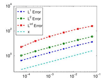
Figure 1. Spatial convergence orders in the $L^{1}$, $L^{2}$, and $L^{\infty}$ norm.

8.2. Decay rates

According to Theorem 4, the solution to the Keller-Segel system converges to the homogeneous steady state if $\mu$ or $1/\delta$ are sufficiently small. We will verify this property experimentally. To this end, let $\Omega=(-\frac{1}{2},\frac{1}{2})^{2}$ and

$$n_{0}(x,y)=\frac{M}{2\pi\theta}\exp\left(-\frac{x^{2}+y^{2}}{2\theta}\right),$$

where $\theta=10^{-2}$ and $M=5\pi$. We compute the approximate solution on a $32\times 32$ Cartesian grid, and we choose $\Delta t=2\cdot 10^{-4}$. In Figure 2, we depict the temporal evolution of the relative entropy $E^{*}(t^{k})=E[n^{k}|n^{*}]$ in semi-logarithmic scale. In all cases shown, the convergence seems to be of exponential rate. The rate becomes larger for larger values of $\delta$ or smaller values of $\mu$ which is in agreement with estimate (32). In fact, the constant $C^{*}$ is proportional to $\mu^{2}/\delta$ (see Theorem 4) and the rate improves if $\mu^{2}/\delta$ is smaller.

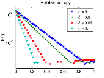
(a) $\mu=1$.

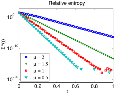
(b) $\delta=10^{-3}$.

Figure 2. Relative entropy $E[n^{k}|n^{*}]$ versus time $t^{k}$ in semi-logarithmic scale for various values of $\delta$ and $\mu$.

As a numerical check, we computed the evolution of the relative entropies for different grid sizes $N$ and different time step sizes $\Delta t$. Figure 3 shows that the decay rate does not depend on the time step or the mesh considered.

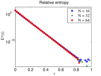
(a) $\Delta t=2.10^{-5}$.

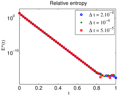
(b) $N=16$.

Figure 3. Relative entropy $E[n^{k}|n^{*}]$ versus time $t^{k}$ in semi-logarithmic scale for various mesh and time step sizes.

8.3. Nonsymmetric initial data on a square

In this subsection, we explore the behavior of the solutions to (1) for different values of $\delta$. We choose $\Omega=(-\frac{1}{2},\frac{1}{2})^{2}$ with a $64\times 64$ Cartesian grid, $\mu=1$, and $\Delta t=2\cdot 10^{-5}$. We consider two nonsymmetric initial functions with mass $6\pi$:

(33) $$n_{0,1}(x,y) =\frac{6\pi}{2\pi\theta}\exp\left(-\frac{(x-x_{0})^{2}+(y-y_{0})^{2}}{2\theta}\right),$$

(34) $$n_{0,2}(x,y) =\frac{4\pi}{2\pi\theta}\exp\left(-\frac{(x-x_{0})^{2}+(y-y_{0})^{2}}{2\theta}\right)+\frac{2\pi}{2\pi\theta}\exp\left(-\frac{(x-x_{1})^{2}+(y-y_{1})^{2}}{2\theta}\right),$$

where $\theta=10^{-2}$, $x_{0}=y_{0}=0.1$, and $x_{1}=y_{1}=-0.2$ (see Figure 4).

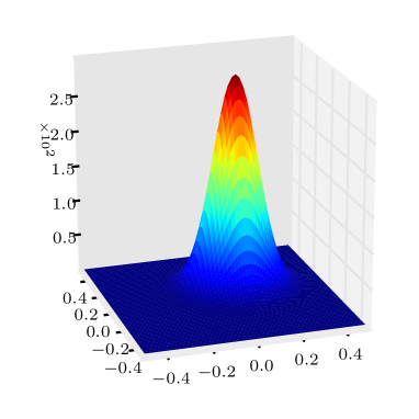
(a) Initial datum $n_{0,1}$.

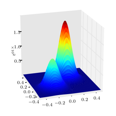
(b) Initial datum $n_{0,2}$.

Figure 4. Initial cell densities.

We consider first the case $\delta=0$, which corresponds to the classical parabolic-elliptic Keller-Segel system. In this case, our finite volume scheme coincides with that of [16]. We recall that solutions to the classical parabolic-elliptic model blow up in finite time if the initial mass satisfies $M>4\pi$ [27] (in the non-radial case). The numerical results at a time just before the numerical blow-up are presented in Figure 5. We observe the blow-up of the cell density in finite time, and the blow-up occurs at the boundary, as expected. More precisely, it occurs at that corner which is closest to the global maximum of the initial datum.

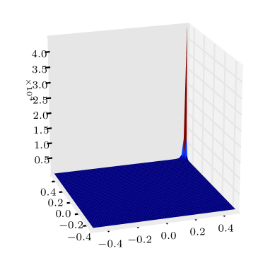
(a) Initial datum $n_{0,1}$, $t=1$.

(b) Initial datum $n_{0,2}$, $t=0.6$.

Figure 5. Cell density computed from nonsymmetric initial data with $M=6\pi$ and $\delta=0$.

Next, we choose $\delta=10^{-3}$ and $\delta=10^{-2}$. According to Theorem 1, the numerical solution exists for all time. This behavior is confirmed in Figure 6, where we show the cell density at time $t=5$. At this time, the solution is very close to the steady state which is nonhomogeneous. We observe a smoothing effect of the cross-diffusion parameter $\delta$; the cell density maximum decreases with increasing values of $\delta$.

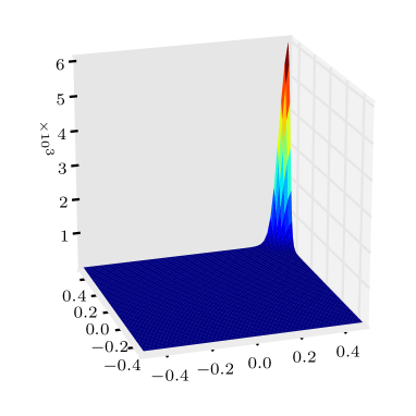
(a) Initial datum $n_{0,1}$, $\delta=10^{-3}$.

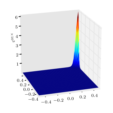
(b) Initial datum $n_{0,2}$, $\delta=10^{-3}$.

(c) Initial datum $n_{0,1}$, $\delta=10^{-2}$.

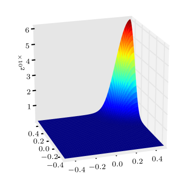
(d) Initial datum $n_{0,2}$, $\delta=10^{-2}$.

Figure 6. Cell density computed at $t=5$ from nonsymmetric initial data with $M=6\pi$ for different values of $\delta$.

8.4. Symmetric initial data on a square

We consider, as in the previous subsection, the domain $\Omega=(-\frac{1}{2},\frac{1}{2})^{2}$ with a $64\times 64$ Cartesian grid, $\mu=1$, and $\Delta t=10^{-5}$. Here, we consider the radially symmetric initial datum

(35) $$n_{0,3}(x,y)=\frac{M}{2\pi\theta}\exp\left(-\frac{x^{2}+y^{2}}{2\theta}\right)$$

with $M=20\pi$ and $\theta=10^{-2}$. Since $M>8\pi$ and the initial datum is radially symmetric, we expect that the solution to the classical Keller-Segel model ($\delta=0$) blows up in finite time [26, 30]. Figure 7 shows that this is indeed the case, and blow-up occurs in the center of the domain.

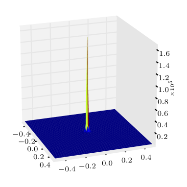
Figure 7. Cell density at time $t=0.05$ computed from to the radially symmetric initial datum $n_{0,3}$ with $M=20\pi$ and $\delta=0$.

In contrast to the classical Keller-Segel system, when taking $\delta=10^{-3}$, the cell density peak moves to a corner of the domain and converges to a nonhomogeneous steady state (see Figure 8). The time evolution of the $L^{\infty}$ norm of the cell density shows an interesting behavior (see Figure 9). We observe two distinct levels. The first one is reached almost instantaneously. The $L^{\infty}$ norm stays almost constant and the cell density seems to stabilize at an intermediate symmetric state (Figure 8a). After some time, the $L^{\infty}$ norm increases sharply and the cell density peak moves to the boundary (Figure 8b). Then the solution stabilizes again (Figure 8c). We note that we obtain the same steady state when using a Gaussian centered at $(-10^{-3},-10^{-3})$.

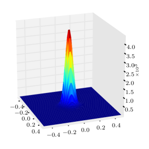
(a) $t=0.6$.

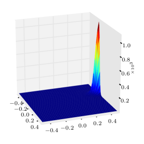
(b) $t=0.73$.

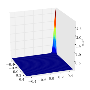
(c) $t=5$.

Figure 8. Cell density computed from the radially symmetric initial datum $n_{0,3}$ with $M=20\pi$ and $\delta=10^{-3}$.

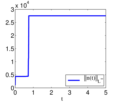
Figure 9. Time evolution of $\|n^{k}\|_{L^{\infty}(\Omega)}$ computed from the radially symmetric initial datum $n_{0,3}$ with $M=20\pi$ and $\delta=10^{-3}$.

8.5. Nonsymmetric initial data on a rectangle

We consider the domain $\Omega=(-1,1)$ $\times(-\frac{1}{2},\frac{1}{2})$ and compute the approximate solutions on a $128\times 64$ Cartesian grid with $\Delta t=5\cdot 10^{-5}$. The secretion rate is again $\mu=1$, and we choose the initial data $n_{0,1}$ and $n_{0,2}$, defined in (33)-(34) with mass $M=6\pi$. If $\delta=0$, the solution blows up in finite time and the blow up occurs in a corner as in the square domain (see Figure 10). If $\delta=10^{-3}$, the approximate solutions converge to a non-homogeneous steady state (Figure 11). Interestingly, before moving to the corner, the solution evolving from the nonsymmetric initial datum $n_{0,2}$ shows some intermediate behavior; see Figure 11b.

(a) Initial datum $n_{0,1}$, $t=0.5$.

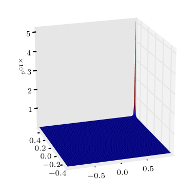
(b) Initial datum $n_{0,2}$, $t=1.7$.

Figure 10. Cell density computed from nonsymmetric initial data with $M=6\pi$ and $\delta=0$.

(a) Initial datum $n_{0,1}$, $t=1$.

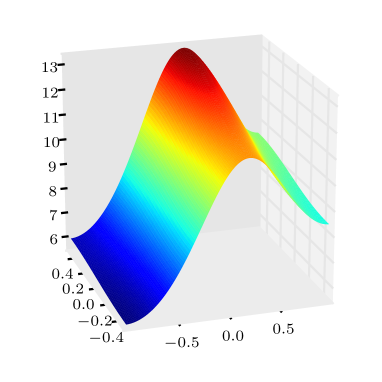
(b) Initial datum $n_{0,2}$, $t=1$.

(c) Initial datum $n_{0,1}$, $t=5$.

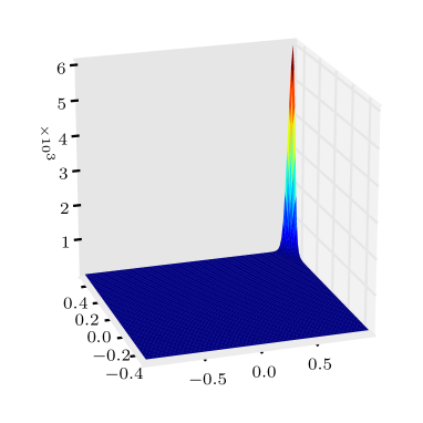
(d) Initial datum $n_{0,2}$, $t=5$.

Figure 11. Cell density computed from nonsymmetric initial data with $M=6\pi$ and $\delta=10^{-3}$.

8.6. Symmetric initial data on a rectangle

The domain is still the rectangle $\Omega=(-1,1)\times(-\frac{1}{2},\frac{1}{2})$, we take a $128\times 64$ Cartesian grid, $\mu=1$, and $\Delta t=10^{-5}$. We choose the initial datum $n_{0,3}$, defined in (35), with $M=20\pi$. Clearly, the approximate solution to the classical Keller-Segel model $\delta=0$ blows up in finite time in the center $(0,0)$ of the rectangle. When $\delta=10^{-3}$, the cell density peak first moves to the closest boundary point before moving to a corner of the domain, as in the square domain (Figure 12). However, in contrast to the case of a square domain, there exist two intermediate states, one up to time $t\approx 0.9$ and another in the interval $(0.9,2.3)$, and one final state for long times (see Figure 13). We note that the same qualitative behavior is obtained using $\delta=10^{-2}$.

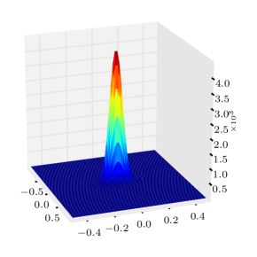
(a) $t=0.7$.

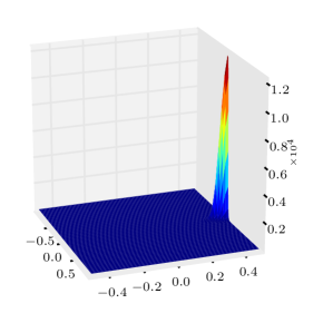
(b) $t=1.9$.

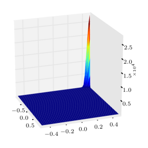
(c) $t=2.5$.

Figure 12. Cell density computed from the symmetric initial datum $n_{0,3}$ with $M=20\pi$ and $\delta=10^{-3}$.

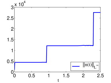
Figure 13. Time evolution of $\|n^{k}\|_{L^{\infty}(\Omega)}$ computed from the radially symmetric initial datum $n_{0,3}$ with $M=20\pi$ and $\delta=10^{-3}$.

References

- [1] M. Bessemoulin-Chatard, C. Chainais-Hillairet, and F. Filbet. On discrete functional inequalities for some finite volume schemes. Submitted for publication, 2012. http://arxiv.org/abs/1202.4860.
- [2] A. Blanchet, V. Calvez, and J. A. Carrillo. Convergence of the mass-transport steepest descent scheme for the subcritical Patlak-Keller-Segel model. SIAM J. Numer. Anal. 46 (2008), 691-721.
- [3] A. Blanchet, E. Carlen, and J. A. Carrillo. Functional inequalities, thick tails and asymptotics for the critical mass Patlak-Keller-Segel model. J. Funct. Anal. 261 (2012), 2142-2230.
- [4] A. Blanchet, J. A. Carrillo, and N. Masmoudi. Infinite time aggregation for the critical Patlak-Keller-Segel model in . Comm. Pure Appl. Math. 61 (2008), 1449-1481.
- [5] A. Blanchet, J. Dolbeault, and B. Perthame. Two-dimensional Keller-Segel model: Optimal critical mass and qualitative properties of the solutions. Electr. J. Diff. Eqs. 44 (2006), 1-33.
- [6] C. Budd, R. Carretero-González, and R. Russell. Precise computations of chemotactic collapse using moving mesh methods. J. Comput. Phys. 202 (2005), 463-487.
- [7] M. Burger, J. A. Carrillo, and M.-T. Wolfram. A mixed finite element method for nonlinear diffusion equations. Kinetic Related Models 3 (2010), 59-83.
- [8] M. Cáceres, J. A. Carrillo, and J. Dolbeault. Nonlinear stability in for a confined system of charged particles. SIAM J. Math. Anal. 34 (2002), 478-494.
- [9] J. A. Carrillo, S. Hittmeir, and A. Jüngel. Cross diffusion and nonlinear diffusion preventing blow up in the Keller-Segel model. To appear in Math. Mod. Meth. Appl. Sci., 2012.
- [10] C. Chainais-Hillairet, J.-G. Liu, and Y.-J. Peng. Finite volume scheme for multi-dimensional drift-diffusion equations and convergence analysis. Math. Mod. Numer. Anal. 37 (2003), 319-338.
- [11] A. Chertock and A. Kurganov. A second-order positivity preserving central-upwind scheme for chemotaxis and haptotaxis models. Numer. Math. 111 (2008), 169-205.
- [12] L. Desvillettes and K. Fellner. Entropy methods for reaction-diffusion equations with degenerate diffusion arising in reservible chemistry. Preprint, 2007. http://www.uni-graz.at/fellnerk.
- [13] M. Dreher and A. Jüngel. Compact families of piecewise constant functions in . Nonlin. Anal. 75 (2012), 3072-3077.
- [14] Y. Epshteyn and A. Izmirlioglu. Fully discrete analysis of a discontinuous finite element method for the Keller-Segel chemotaxis model. J. Sci. Comput. 40 (2009), 211-256.
- [15] R. Eymard, T. Gallouët, and R. Herbin. Finite volume methods. In: P. G. Ciarlet and J. L. Lions (eds.). Handbook of Numerical Analysis, Vol. 7. North-Holland, Amsterdam (2000), 713-1020.
- [16] F. Filbet. A finite volume scheme for the Patlak-Keller-Segel chemotaxis model. Numer. Math. 104 (2006), 457-488.
- [17] A. Guionnet and B. Zegarlinski. Lectures on logarithmic Sobolev inequalities. In: J. Azéma et al. (eds.), Séminaire de Probabilités, Vol. 36, pp. 1-134, Lect. Notes Math. 1801, Springer, Berlin, 2003.
- [18] J. Haškovec and C. Schmeiser. Stochastic particle approximation for measure valued solutions of the 2D Keller-Segel system. J. Stat. Phys. 135 (2009), 133-151.
- [19] J. Haškovec and C. Schmeiser. Convergence of a stochastic particle approximation for measure solutions of the 2D Keller-Segel system. Commun. Part. Diff. Eqs. 36 (2011), 940-960.
- [20] M. Herrero and J. Velázquez. Singularity patterns in a chemotaxis model. Math. Annalen 306 (1996), 583-623.
- [21] T. Hillen and K. Painter. A user’s guide to PDE models for chemotaxis. J. Math. Biol. 58 (2009), 183-217.
- [22] S. Hittmeir and A. Jüngel. Cross diffusion preventing blow-up in the two-dimensional Keller-Segel model. SIAM J. Math. Anal. 43 (2011), 997-1022.
- [23] W. Jäger and S. Luckhaus. On explosions of solutions to a system of partial differential equations modelling chemotaxis. Trans. Amer. Math. Soc. 329 (1992), 819-824.
- [24] E. Keller and L. Segel. Initiation of slime mold aggregation viewed as an instability. J. Theor. Biol. 26 (1970), 399-415.
- [25] A. Marrocco. Numerical simulation of chemotactic bacteria aggregation via mixed finite elements. Math. Mod. Numer. Anal. 4 (2003), 617-630.
- [26] T. Nagai. Blow-up of radially symmetric solutions to a chemotaxis system. Adv. Math. Sci. Appl. 5 (1995), 581-601.
- [27] T. Nagai. Blowup of nonradial solutions to parabolic-elliptic systems modeling chemotaxis in two-dimensional domains. J. Inequal. Appl. 6 (2001), 37-55.
- [28] T. Nagai, T. Senba, and K. Yoshida. Application of the Trudinger-Moser inequality to a parabolic system of chemotaxis. Funkcial. Ekvac. 40 (1997), 411-433.
- [29] C. Patlak. Random walk with persistence and external bias. Bull. Math. Biophys. 15 (1953), 311-338.
- [30] B. Perthame. PDE models for chemotactic movements. Parabolic, hyperbolic and kinetic. Appl. Math. 49 (2005), 539-564.
- [31] B. Perthame. Transport Equations in Biology. Birkhäuser, Basel, 2007.
- [32] N. Saito. Conservative upwind finite-element method for a simplified Keller-Segel system modelling chemotaxis. IMA J. Numer. Anal. 27 (2007), 332-365.
- [33] N. Saito. Error analysis of a conservative finite-element approximation for the Keller-Segel model of chemotaxis. Comm. Pure Appl. Anal. 11 (2012), 339-364.
- [34] N. Saito and T. Suzuki. Notes on finite difference schemes to a parabolic-elliptic system modelling chemotaxis. Appl. Math. Comput. 171(2005), 72-90.
- [35] R. Strehl, A. Sokolov, D. Kuzmin, and S. Turek. A flux-corrected finite element method for chemotaxis problems. Comput. Meth. Appl. Math. 10 (2010), 219-232.
- [36] R. Tyson, L. Stern, and R. LeVeque. Fractional step methods applied to a chemotaxis model. J. Math. Biol. 41 (2000), 455-475.