High-Resolution Spectroscopy During Eclipse of the Young Substellar Eclipsing Binary 2MASS 0535$-$0546. II. Secondary Spectrum: No Evidence that Spots Cause the Temperature Reversal

Abstract

We present high-resolution optical spectra of the young brown-dwarf eclipsing binary 2M0535$-$05, obtained during eclipse of the higher-mass (primary) brown dwarf. Combined with our previous spectrum of the primary alone (Paper I), the new observations yield the spectrum of the secondary alone. We investigate, through a differential analysis of the two binary components, whether cool surface spots are responsible for suppressing the temperature of the primary. In Paper I, we found a significant discrepancy between the empirical surface gravity of the primary and that inferred via fine analysis of its spectrum. Here we find precisely the same discrepancy in surface gravity, both qualitatively and quantitatively. While this may again be ascribed to either cool spots or model opacity errors, it implies that cool spots cannot be responsible for preferentially lowering the temperature of the primary: if they were, spot effects on the primary spectrum should be preferentially larger, and they are not. The $T_{\rm eff}$ we infer for the primary and secondary, from the TiO-$\epsilon$ bands alone, show the same reversal, in the same ratio, as is empirically observed, bolstering the validity of our analysis. In turn, this implies that if suppression of convection by magnetic fields on the primary is the fundamental cause of the $T_{\rm eff}$ reversal, then it cannot be a local suppression yielding spots mainly on the primary (though both components may be equally spotted), but a global suppression in the interior of the primary. We briefly discuss current theories of how this might work.

1 Introduction: Results for 2M0535 So Far

2MASS 05352184$-$0546085 (hereafter 2M0535) is a very young system located in the Orion Nebula Cluster, and identified by Stassun et al. (2006, hereafter SMV06) as the first known substellar eclipsing binary (EB). EBs allow extremely precise direct measurements (via their orbital dynamics and eclipse lightcurves) of the component masses and radii, and hence their surface gravities ($\log g$), as well as the ratio of their luminosities (and thus the ratio of their effective temperatures, $T_{\rm eff}$). 2M0535 therefore enables one to rigorously test the evolutionary models and synthetic spectra that are widely used to characterize the vast majority of brown dwarfs (for which a direct determination of mass and radius is not possible), and to do so at the young ages where our theoretical knowledge is most lacking.

The measurements by SMV06 were refined by Stassun et al. (2007) and Gómez Maqueo Chew et al. (2009, hereafter G09). The central results are: (1) Both components of 2M0535 are moderate mass brown dwarfs ($M_{\rm A}=0.0572\pm 0.0033\,M_{\odot}$, $M_{\rm B}=0.0366\pm 0.0022\,M_{\odot}$); (2) their radii ($R_{\rm A}=0.690\pm 0.011R_{\odot}$, $R_{\rm B}=0.540\pm 0.009R_{\odot}$) are consistent with the theoretical expectation that young brown dwarfs should be much larger than their field counterparts; and (3) the $T_{\rm eff}$ ratio of the components ($T_{\rm eff,B}/T_{\rm eff,A}=1.050\pm 0.004$) shows a surprising reversal, with the more massive primary (A) being cooler than the secondary (B).

The $T_{\rm eff}$ reversal is not predicted by any current set of theoretical evolutionary tracks. To explain it, Chabrier et al. (2007, henceforth CGB07) proposed that strong magnetic fields on the primary suppress convection, both globally in the interior, and/or locally near the surface (producing cool surface spots); neither effect is included in standard evolutionary models, and both would act to depress the effective temperature of the primary. MacDonald & Mullan (2009, hereafter MM09) subsequently put forward a qualitatively similar hypothesis, wherein magnetic fields lower the $T_{\rm eff}$ of the primary by inhibiting interior convection (though their theory differs in important respects from that of CGB07, as we discuss later).

Bolstering the case for strong magnetic fields preferentially affecting the primary, Reiners et al. (2007) found that, compared to the secondary, the primary is a relatively rapid rotator (which should boost field generation), with very prominent chromospheric H$\alpha$ emission (ultimately powered by the release of magnetic stresses). Mohanty et al. (2009) subsequently showed, through an analysis of the optical to mid-infrared spectral energy distribution of 2M0535, that ongoing disk accretion is highly improbable in this system. Thus the H$\alpha$ emission in the primary is indeed likely to be chromospheric in origin, supporting Reiners et al.’s conclusion that it harbors strong magnetic fields. Interestingly, these results are also consistent with the behaviour of low-mass field stars: chromospherically active late-K and M field dwarfs appear cooler than inactive ones of the same luminosity (Morales et al., 2008; Stassun et al., 2012).

The implication is that magnetic fields appear to have a large impact on the effective temperature of low-mass stars and brown dwarfs. If true, this would have far-reaching consequences for our understanding of these objects. For example, the initial mass function (IMF) in young star-forming regions is often derived by comparing (sub)stellar luminosities and temperatures to theoretical HR diagrams. The latter do not include any field effects, while a substantial fraction of low-mass stars and brown dwarfs at these very early ages show evidence of strong fields (rapid rotation and high activity), just like 2M0535A and active field dwarfs; thus, the inferred IMF might be skewed by a field-induced depression in $T_{\rm eff}$, potentially causing an overestimate of the number of low-mass brown dwarfs.

The issue now is to decipher how exactly fields achieve this effect, if indeed they are responsible. As noted above, theory suggests they might do so by producing cool surface spots (through local suppression of convection), and/or by inhibiting convection globally in the (sub)stellar interior. Observationally, checking for the presence of spots is clearly easier. G09 carried out the first investigation of spots on 2M0535AB. They showed that the small amplitude residual (non-eclipse) variations in the system’s lightcurve, modulated at the rotational periods of the primary and secondary, can be well-reproduced by cool spots asymmetrically covering a small fraction ($\lesssim$ 10%) of both components’ surfaces. While they find no evidence for a large ($\gtrsim$ 50%) spot coverage preferentially on the primary, as required by CGB07’s theory if spots are to account for the $T_{\rm eff}$ reversal, they cannot rule out such spots either, if the latter are arranged symmetrically about the primary’s rotation axis (e.g., polar spots, latitudinal bands, or “leopard spots”).

To check for spots independent of their orientation, one must examine the spectra of the binary components. Cool spots are by definition cooler than the surrounding photosphere, and the effective surface gravity within them is also lower (because the magnetic pressure partly offsets the gas pressure, mimicking the reduction in gas pressure caused by a lower surface gravity); both effects alter the shape of temperature- and gravity- (more accurately, gas-pressure-) sensitive spectral lines relative to an unspotted spectrum. We embarked upon this study in a previous paper (Mohanty et al., 2010, hereafter Paper I), where we analysed the high-resolution optical spectrum of the primary 2M0535A alone (obtained during secondary eclipse, with a negligible 1.6% contamination by the secondary). Specifically, we derived $T_{\rm eff}$ and $\log g$ by simultaneously fitting the observed TiO-$\epsilon$ band and red lobe of the KI doublet with state-of-the-art synthetic spectra, and compared our results to the empirically known $\log g$. We found that at the $T_{\rm eff}$ $\approx$ 2500 K inferred from TiO, the KI lobe implies $\log g$ $\approx$ 3.0, or 0.5 dex lower than the empirical value. Conversely, at the known $\log g$ of 3.5, the $T_{\rm eff}$ inferred from K I is 2650 K, or 150 K higher than derived from TiO.

Such discrepancies are indeed expected if the photosphere is spotted, due to the temperature and effective gravity properties of spots noted above. In particular, we showed that the spectrum of 2M0535A is consistent with an unspotted stellar photosphere with $T_{\rm eff}$ = 2700 K and (empirical) $\log g$ = 3.5, coupled with axisymmetric cool spots that are 15% cooler (2300 K), have an effective $\log g$ = 3.0 (0.5 dex lower than photospheric) and cover 70% of the surface. The spot temperature and gravity are consistent with the properties of sunspots and starspots in general, as well as with the previous lightcurve analysis of 2M0535, while the covering fraction agrees with CGB07’s requirement if spots are to cause the $T_{\rm eff}$ reversal.

On the other hand, these discrepancies may arise from errors in the molecular opacities or equation of state (EOS) in the synthetic spectra we used to fit the data. Such errors are known to be present from analyses of field dwarfs (Reiners et al., 2005); while it is unclear whether they persist in the model spectra at the much lower $\log g$ appropriate for very young brown dwarfs, it is certainly possible (see Paper I).

2 Goal of This Paper

In either case, a resolution demands an analogous analysis of the spectrum of the secondary, 2M0535B. That is our goal here. If a large covering fraction of spots is preferentially affecting the primary, then the much less spotted secondary should evince much smaller spectral discrepancies, if any. If opacity/EOS errors are to blame instead, then the secondary should show similar discrepancies: since its empirical $\log g$ is nearly the same as the primary’s, and so is its $T_{\rm eff}$ (as implied by an empirical $T_{\rm eff}$ ratio very close to unity), opacity/EOS uncertainties in the model spectra should affect our analyses of both components to a similar degree. Note that, in the latter case, one cannot appeal to real spot effects on the primary simply being washed out by model errors. As discussed above, the primary spot covering fraction required to produce the $T_{\rm eff}$ reversal is of the same order as inferred from its spectrum under the assumption of error-free models; if model errors are in fact large enough to overwhelm spot effects, then such spots are automatically too small to cause the reversal. Finally, the secondary may also exhibit similar (or larger) discrepancies if it is as (or more) spotted than the primary. In this case too, spots can be excluded as the cause of the $T_{\rm eff}$ reversal, since the latter requires the primary to be far more spotted than the secondary.

To summarize, our aim is to investigate whether the secondary spectrum shows much smaller discrepancies than the primary; if it does, then spots on the primary are favoured as the mechanism for $T_{\rm eff}$ reversal, otherwise such spots can be effectively ruled out.

3 Observations and Data Reduction

The data collection and reduction for the observation of the primary eclipse were performed in precisely the same manner, using the same instrumental setup and procedures, as for our previous observation and analysis of the secondary eclipse (Paper I). Here we briefly summarize the salient details.

We observed 2M0535 on the night of UT 2011 March 15 with the High Resolution Echelle Spectrometer (HIRES) on Keck-I. We observed in the spectrograph’s “red” (HIRESr) configuration with an echelle angle of $-0.403$ deg and a cross-disperser angle of 1.7035 deg. In this configuration, the two features of primary interest in this paper, TiO $\lambda\lambda$8435–8455 and K I $\lambda$7700, fall on the “green” chip, in echelle orders 42 and 46, respectively. We used the OG530 order-blocking filter and the 1$\farcs$15$\times$7$\farcs$0 slit, and binned the chip during readout by 2 pixels in the dispersion direction. The resulting resolving power is $R\approx 34\,000$, with a 3.7-pixel ($\sim 8.8$ km s^-1) FWHM resolution element.

We obtained three consecutive integrations of 2M0535, each of 2400 s. ThAr arc lamp calibration exposures were obtained before and after the 2M0535 exposures, and sequences of bias and dome flat-field exposures were obtained at the beginning of the night. The 2M0535 exposures were processed along with these calibrations using standard IRAF tasks and the makee reduction package written for HIRES by T. Barlow. The latter includes optimal extraction of the orders as well as subtraction of the adjacent sky background. The three exposures of 2M0535 were processed separately and then median combined with cosmic-ray rejection into a single final spectrum. The signal-to-noise (S/N) of the final spectrum is $\sim 15$ per resolution element.

To complement our observation of the secondary eclipse in Paper I, here we intentionally chose the observations to coincide exactly with the primary eclipse, i.e. when the higher-mass, larger, lower-$T_{\rm eff}$ primary component was behind the secondary as seen from Earth. The first exposure started at UT 05:51 hr, and the third exposure ended at UT 07:54 hr, corresponding to orbital phases of 0.7371 and 0.7458, respectively, during which time the primary is maximally blocked (cf. Fig. 3 in Stassun et al., 2007). Integrated over the entire 2-hr observation, the total light contribution from the blocked primary was $\approx$35.1%, calculated using the accurately determined radius ratio, temperature ratio, and orbital parameters, including the orbital inclination, from the light curve modeling performed in G09.

Given the exorbitant time cost of the observations and the difficulty in scheduling at precisely the right phase, it was not feasible to obtain multiple observations for this project. However, the extensive light curve observations of Stassun et al. (2006, 2007) and G09, spanning more than 10 years, clearly demonstrate that the system is not variable outside of eclipse at more than $\sim$10%. So we have good reason to believe that the observation presented here should be adequately representative.

4 Methodology

4.1 Isolation of the secondary spectrum

For our analysis, we require the spectrum of the lower-mass component (the “secondary”) of 2M0535 alone, i.e., as uncontaminated by light from the primary component as possible. In Paper I, we observed the 2M0535 system during secondary eclipse, i.e., when the primary component was in front of the secondary. The secondary eclipse is near total, and thus our observations in Paper I provided a “pure” measurement of the primary component’s spectrum, with a negligible 1.6% contamination from the secondary component.

The spectrum that we have obtained here of the secondary component is much less pure—it is 35.1% contaminated by the primary’s light (see above)—because the primary eclipse is not total. Thus, we have used our isolated spectrum of the primary component from Paper I to correct the observed spectrum of the secondary component. Specifically, we shifted the isolated primary spectrum in velocity according to the known ephemeris of the system (see G09), scaled it to 35.1% of the total light, and subtracted it from the observed spectrum of the secondary. Because this procedure involves subtraction of two observed spectra with comparable S/N, the S/N of the resulting final isolated spectrum of the secondary is decreased to $\sim 10$.

4.2 Synthetic spectra

In order to conduct an analysis identical to that in Paper I, we use a subset of the same atmospheric models adopted in that paper. Specifically, we use synthetic spectra for plane-parallel atmospheres generated using the PHOENIX code, designated AMES-Cond (version 2.4 Allard et al., 2001). As in our analysis of the primary, we use solar-metallicity models ($[M/H]=0.0$). While the metallicity of 2M0535 is not explicitly known, a large deviation from solar is not expected for a young object in a nearby star-forming region.

Note that in Paper I, we considered AMES-Dusty as well as AMES-Cond models. Both treat the formation of dust grains self-consistently, through chemical equilibrium calculations. Once formed, however, the grains are assumed to remain entirely suspended in the photosphere in the Dusty models, and settle completely below the photosphere in the Cond ones. Under physical conditions where the chemical equations imply no dust formation, the Cond and Dusty spectra are identical; in the models, this occurs for $T_{\rm eff}$ $\geq$ 2500 K. For the latter temperatures, therefore, either set of models may be used. In Paper I, we used Dusty models for $T_{\rm eff}$ $<$ 2500 K (i.e., in the dust formation regime; for late M-types with grains, Dusty models are expected to be more appropriate than Cond, since grains are expected to start settling out of the atmosphere only around mid-to-late L types), and Cond models for $T_{\rm eff}$ $\geq$ 2500 K (since either Cond or Dusty can be used in this grainless regime, and the high-resolution Cond spectra available to us extend to higher $T_{\rm eff}$ than the Dusty ones). In the present paper, concerned with investigating the secondary component of 2M0535, we use only the (grainless) Cond models at $T_{\rm eff}$ $>$ 2500 K, since the secondary is warmer than the primary considered in Paper I, and is definitely hotter than $\sim$2500 K (see Mohanty et al., 2009).

4.3 Determination of $T_{\rm eff}$ and $\log g$

Our goal is to determine the $T_{\rm eff}$ and $\log g$ of the lower-mass component of 2M0535 (the “secondary,” hereafter 2M0535B) from comparisons to synthetic spectra. As in Paper I, we again follow (Mohanty et al., 2004, hereafter M04), who have shown that two ideal regions for this analysis are the TiO- bandheads at $\lambda\lambda\lambda$8435, 8445, 8455, and the red lobe of the K Idoublet at $\lambda$7700 (the blue lobe falls in the gap between echelle orders in the HIRES setting used). In particular, the TiO bandheads are very sensitive to $T_{\rm eff}$, but negligibly so to $\log g$, while the K I absorption is sensitive to both; using the two regions in tandem therefore enables one to disentangle and individually determine these two parameters, as we did for the 2M0535A component in Paper I.

The synthetic spectra were treated for comparison to the data precisely as in Paper I. Briefly, the model spectra were broadened by the instrumental profile, and interpolated onto the wavelength scale of the data. Since our data are not flux calibrated, both the data and models were then normalized over a selected pseudo-continuum interval, just outside the TiO-$\epsilon$ and K I bands of interest, for comparison: over $\lambda\lambda$[8405.0–8414.0] for TiO, and $\lambda\lambda$[7693.0–7698.0] for K I. The only change from Paper I is that no rotational broadening of the synthetic spectra was required in the present case, since the slowly-rotating 2M0535B is effectively unbroadened ($v\sin i<5$ km s^-1; Reiners et al., 2007) compared to the instrumental resolution (8.8 km s^-1; see above). Finally, we note, as in Paper I, that the models were originally constructed at intervals of 100 K and 0.5 dex in $T_{\rm eff}$ and $\log g$, respectively, so we have linearly interpolated between adjacent spectra to construct a finer final grid of models, with steps of 50 K in $T_{\rm eff}$ and 0.25 dex in $\log g$.

5 Results

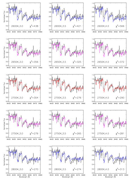
Figure 1: Observed TiO-$\epsilon$ region in 2M0535B (black) compared to Cond models (Allard et al., 2001). Best-fit models shown in red; worse but still admissible fits by eye shown in magenta; and all others, which clearly diverge from the data by eye, shown in blue. The by-eye fits prefer $T_{\rm eff}$ $\approx$ 2700$\pm$50 K. Note that the model fits are relatively insensitive to gravity over the 1 dex range plotted; see Section 5. The corresponding $\chi^{2}$ values for the model fits are also shown in each panel. Note that the best-fit $\chi^{2}$ models (2700–2800 K) are $\sim$50 K hotter than the best-fit models by eye (2650–2750 K); this is because the cores of the bandheads are better fit by the slightly cooler models, but the flux in these spectral regions is weighted less in the $\chi^{2}$ fits to account for lower S/N there. The best-fit models from the two methods are nevertheless consistent with each other, given the $\sim$50 K uncertainty in the by-eye fits; see §5.

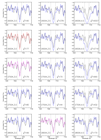
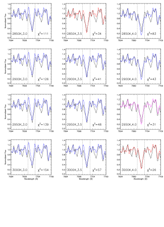
Figure 2: Observed red lobe of K I in 2M0535B (black) compared to Cond models (Allard et al., 2001). From top to bottom, the three columns on the left depict model $T_{\rm eff}$ from 2600 to 2800 K, and the three columns on the right show $T_{\rm eff}$ from 2850 to 3000 K. Best-fit models by eye are shown in red; worse but still admissible fits by eye are shown in magenta; and all others, which clearly diverge from the data, are shown in blue. Note that the K I absorption is sensitive to both $T_{\rm eff}$ and gravity: a 150 K increase in $T_{\rm eff}$ compensates for a 0.5 dex rise in log g. At $T_{\rm eff}$ = 2700 K, corresponding to the best-fit by eye to TiO-$\epsilon$ (Figure 1), the K I by-eye fit implies $\log g$ = 3.0, while at the empirically determined $\log g$ = 3.5, it implies $T_{\rm eff}$ = 2850 K. At the still higher gravity of $\log g$ = 4.0, the best model fit by eye is at 3000 K, but this gravity is empirically ruled out. The corresponding $\chi^{2}$ values are also shown in each panel; the best-fit models implied by these values are in good agreement with the by-eye results. See Section 5.

The models are overplotted on the data in Figs. 1 and 2, for TiO and K I respectively, over the range of model $T_{\rm eff}$ and $\log g$ plausible for this cool and very young (low-gravity) object. To guide the eye better, both the synthetic and observed spectra have been boxcar-smoothed by 3 pixels in these plots. Models that best fit the data, by eye, are plotted in red, marginally worse fits in magenta, and bad fits in blue. We note the following trends.

TiO-$\epsilon$: Fig. 1 shows that, as expected, the TiO-$\epsilon$ bandheads are quite insensitive to gravity, over the range in $\log g$ shown, but highly sensitive to temperature. The best fit by eye is obtained to the model at 2700 K (in red), while models within $\pm$50 K of this (in magenta) are marginally worse. Models that are even cooler/hotter (in blue) appear clearly inconsistent with the data: the bandheads at 8445 Å and (especially) 8435 Å are significantly stronger than the data by $T_{\rm eff}$ = 2600 K, while the bandheads at 8445 Å and (especially) 8455 Å are considerably weaker than the data by 2800 K. Since even a 100 K deviation from the best fit is evident to the eye, our precision in $T_{\rm eff}$ determination by eye is likely to be $\sim$50 K (in agreement with M04). From the TiO-$\epsilon$ fits alone, therefore, we would infer $T_{\rm eff}$ $\approx$ 2700$\pm$50 K.

K I and TiO-$\epsilon$: Fig. 2 reveals, again as expected, that the K I line is very sensitive to both $T_{\rm eff}$ and $\log g$, becoming stronger with both decreasing temperature and increasing gravity (the extent of this absorption line – [7700–7703] Å , used for both these by-eye fits and the chi-squared analysis below – is demarcated by the vertical dashed lines in this plot). We see that, at the temperature inferred from TiO (2700$\pm$50 K), the best-fit by eye to K I is at $\log g$ = 3.0 (the best fit here is actually at the lower end of this $T_{\rm eff}$ range, at 2650 K (red); the 2700 K model K I (magenta) is somewhat narrower than the data, while the 2750 K model (blue) is appreciably narrower). At the empirically known gravity of this object, $\log g$ = 3.5, 2700$\pm$50 K models are significantly stronger (broader and deeper) than the data; at this gravity, the best by-eye model fit is obtained at 2850 K (red), which is unsupported by the TiO fits. Finally, for completeness, we also show that at $\log g$ = 4.0, the best fit by eye is at 3000 K (red). The steadily increasing best-fit $T_{\rm eff}$ with increasing $\log g$ simply illustrates the degeneracy between temperature and gravity in the K I line: specifically, an increase of 0.5 dex in $\log g$ is compensated for by an increase of $\sim$150–200 K in $T_{\rm eff}$ (as found my M04). In summary, the best fit to K I at the $T_{\rm eff}$ derived from TiO occurs at a gravity 0.5 dex lower than the known value, while imposing the correct $\log g$ yields a $T_{\rm eff}$ that is $\sim$150 K higher than from TiO, and incompatible with the latter.

To better quantify the fitting results from Figs. 1 and 2, and the uncertainties therein, we carried out chi-square comparisons between the synthetic spectra and data. The TiO comparisons were made over the wavelength range [8420:8480] Å (which includes all three bandheads; see Fig. 1), and the K I ones over [7700.2:7703] Å(corresponding to the entire line, until the pseudo-continuum is reached on either side of line center; see Fig. 2). These ranges correspond to 26 data points for K I and 265 for TiO. The data and models were not smoothed for this exercise, since smoothing introduces correlations between adjacent pixels, thereby vitiating the interpretation of the chi-square vaues. However, the S/N of our data for 2M0535B is lower than that for the primary in Paper I (mainly because, while we compensated for the lower luminosity of the secondary with longer observing times, isolating the secondary spectrum required subtracting the scaled primary spectrum from our data, adding to the noise; see §4.1). This is of concern in the line/bandhead cores, where the flux is lowest, and especially in the K I line core, which is significantly fainter, and thus noisier, than the bottom of the TiO bandheads. To account for this, our chi-square values for individual pixels are weighted by the data pixel flux (for both TiO and K I), effectively making fainter pixels (and thus the line cores) less significant than brighter ones.

The results are plotted in Fig. 3. At the empirical gravity of 2M0535, ($\log g$ = 3.5), the best-fit $T_{\rm eff}$ from K I is 2825 K, in agreement with our by-eye estimate above. The corresponding 1$\sigma$ uncertainty is 35 K. The TiO chi-squares indicate $T_{\rm eff}$ = $2750\pm 15$ K (also at the empirical $\log g$ = 3.5, though these chi-square contours discriminate much less between different gravities than the K I contours, in keeping with the relative insensitivity of TiO to $\log g$). This is again consistent with the by-eye $T_{\rm eff}$ inferred from TiO. Finally, at this $T_{\rm eff}$ and $\log g$ = 3.5, the K I line is marginally fit at the 3$\sigma$ contour level. Given the formal uncertainties in $T_{\rm eff}$ from the TiO and K I chi-squares, the probability that the two $T_{\rm eff}$ at this gravity are equal is only 0.7%. We can thus rule out the possibility that TiO and K I give the same $T_{\rm eff}$ (at the same, empirically determined, $\log g$) with 99.3% confidence.

These results are essentially the same as those obtained in Paper I for 2M0535A: in both the primary and the secondary, the temperatures obtained from TiO-$\epsilon$ and K I are incompatible with each other by $\sim$100–150 K, which is statistically significant at the $\geq$3$\sigma$ level.

We caution that the statistical significance of this discrepancy is formally higher for the primary (see Paper I), because of the lower S/N (equivalently, lower chi-square weighting of the line cores) in the secondary. Thus, our results here should be validated further with higher S/N observations of 2M0535B. Our confidence that our results are not due simply to statistical fluctuations, however, is bolstered by three facts: (a) the qualitative trend for both components is the same: the $T_{\rm eff}$ from TiO is lower than from K I; (b) the quantitative discrepancy between the TiO and K I temperatures is also roughly the same in both cases; and (c) the ratio of component $T_{\rm eff}$ we obtain from TiO, $T_{\rm eff}$_B/$T_{\rm eff}$_A $\approx$ 1.1, is consistent (within the $\pm$50 K spacing in our model $T_{\rm eff}$ grid) with the empirical ratio of 1.05.

6 Discussion

6.1 Implications for Spots Causing $T_{\rm eff}$ Reversal

Assuming that our results are not substantially affected by the lack of high S/N data in the very cores of the lines in the secondary spectrum (as we have argued above they are not), there are only four possible interpretations of the combined analysis presented here and in Paper I.

(1)  Spots are the major cause of the spectral discrepancy in 2M0535A and B. In this case, given that we find the same discrepancy, both qualitatively and quantitatively, in both components, spots cannot be responsible for preferentially depressing the $T_{\rm eff}$ of the primary.

(2)  Opacity/EOS errors cause most of the discrepancy instead. If so, then the spot coverage on the primary would be far too small to produce the $T_{\rm eff}$ reversal: as noted in §2, it is only by ascribing the entire discrepancy in the primary to spots, without considering any model errors, that we get the very large coverage required by CGB07’s spot theory.

(3)  Spots and model errors contribute equally to the discrepancy in each component. In this case, both of the above conclusions would hold: the spot coverage on the primary would be too small, and there would anyway be no marked difference in spottedness between the components, again excluding spots as the cause of the $T_{\rm eff}$ reversal.

(4)  Spots cause the discrepancy in the primary, but model errors, or some other effect, cause it in the secondary. This is unlikely in the extreme, requiring a monumental coincidence. In particular, the empirical $\log g$ of 2M0535A and B are nearly identical, and their $T_{\rm eff}$ are very similar as well (as evinced by the empirical $T_{\rm eff}$ ratio of $\sim$1.05, very close to unity). Model errors would then have to be very prominent at the secondary’s $T_{\rm eff}$ and $\log g$, but disappear over the small parameter jump to the primary, which is improbable; simultaneously, the effects of such errors on the secondary spectrum would have to coincidentally mimic exactly the spot effects on the primary, which is even more unlikely. The same argument applies to any other effect invoked for the secondary but not the primary.

Together, these lines of reasoning imply that, while spots may be present on both 2M0535A and B (and almost certainly are to some extent, as shown by the lightcurve analysis of G09), they cannot be responsible for preferentially lowering the $T_{\rm eff}$ of the primary by a large amount, and thus causing the $T_{\rm eff}$ reversal.

6.2 General Implications for Magnetic Fields Causing $T_{\rm eff}$ Suppression

In light of this result, one might postulate that magnetic fields are not responsible for the temperature reversal at all, and perhaps heating due to tidal interactions (Heller et al. 2010; Gomez Maqueo Chew et al. 2012) is to blame instead. However, with an orbital period of $\sim$10 days, and rotation periods of $\sim$3 days and $\sim$14 days in the primary and secondary respectively (Gomez Maqueo Chew et al. 2009), the two brown dwarfs in 2M0535-05 are sufficiently well separated and sufficiently non-synchronous that significant tidal interactions can be reasonably ruled out (Heller et al. 2010, though a more thorough treatment of the coupled evolution of tidal effects and substellar structure is required to confirm this, as the latter authors note).

On the other hand, even if spots, caused by a local suppression of convection by magnetic fields, are ruled out, fields may still produce the $T_{\rm eff}$ reversal by globally inhibiting convection in the interior of the primary. Both CGB07 and MM09 have proposed such a mechanism. The two theories differ significantly in the interior field strengths invoked, however.

MM09 apply a modified Gough-Taylor instability criterion, in which the magnetic energy basically scales as fraction ($\sim$1–10%) of the total thermal energy, to derive required field strengths of order 10–100 MG in the interior. In more recent work, they derive much smaller fields, but still $\sim$1 MG (MacDonald & Mullan 2012). However, these fields are orders of magnitude greater than the few 10s of kG interior fields, in equipartition with the kinetic (turbulent and convective) energy, suggested by recent simulations (Browning, 2008; Browning et al., 2010). Moreover, interior fields $\gtrsim$ 1 MG may also be buoyantly unstable; more detailed simulations are needed to check if this can be avoided.

Conversely, CGB07 present qualitative physical arguments suggesting that interior fields of $\sim$10 kG (consistent with equipartition with the kinetic energy, and with the recent simulational results cited above) can seriously impede global convection in young brown dwarfs. Within the context of mixing length theory, they find that a convective length scale parameter of $\alpha\ll 0.5$ is required to explain the $T_{\rm eff}$ reversal in 2M0535AB. Testing this, however, requires detailed full 3D simulations of cooling flows along flux tubes in a magnetized convecting medium, which is a considerable undertaking.

Nevertheless, such simulations are essential to discriminate between the theories above, and test whether magnetic fields can indeed inhibit interior convection sufficiently to explain the observed $T_{\rm eff}$ reversal. The rapid pace of advance in simulational complexity (e.g. Browning, 2008; Browning et al., 2010) gives one hope that this will be become a reality in the not-too-distant future. Concurrently, more observations are required to test the universality of such temperature suppression in young very low mass stars and brown dwarfs, not just in eclipsing systems but also in isolated objects. The techniques used by Morales et al. (2008) for field low-mass stars offer a way forward here, though uncertainties in age-dependent luminosities for young objects will simultaneously present a problem in applying these methods. However difficult a task, it must be tackled in order to really understand how magnetic fields affect the fundamental parameters of stars and brown dwarfs.

Figure 3: Determination of goodness-of-fit and formal fit parameter uncertainties. Contours of constant $\chi^{2}-\chi_{\rm min}^{2}=$ 2.3, 6.2, 11.8, representing 1$\sigma$, 2$\sigma$, 3$\sigma$ joint confidence intervals in the $T_{\rm eff}$–$\log g$ parameter plane. Top: joint confidence intervals for fitting of K I. The absolute minimum $\chi^{2}$ best fit is for $T_{\rm eff}$ = 3000 K and $\log g$ = 4.0, however an equally good fit at the 1$\sigma$ level is at $T_{\rm eff}$ = 2825 K and $\log g$ = 3.5 (see Fig. 2). Bottom: joint confidence intervals for fitting of TiO. A best-fit $T_{\rm eff}$ = $2750\pm 15$ K is strongly preferred at high confidence. The best-fit $T_{\rm eff}$ from TiO-$\epsilon$ and K I at the empirical $\log g$ of 3.5 differ by 100–150 K at $\sim 3\sigma$ confidence.

References

- Allard et al. (2001) Allard, F., Hauschildt, P. H., Alexander, D. R., Tamanai, A., & Schweitzer, A. 2001, ApJ, 556, 357
- Browning et al. (2010) Browning, M. K., Basri, G., Marcy, G. W., West, A. A., & Zhang, J. 2010, AJ, 139, 504
- Browning (2008) Browning, M. K. 2008, ApJ, 676, 1262
- Chabrier et al. (2007) Chabrier, G., Gallardo, J., & Baraffe, I. 2007, A&A, 472L, 17 (CGB07)
- Gómez Maqueo Chew et al. (2009) Gómez Maqueo Chew, Y., Stassun, K. G., Prša, A., & Mathieu, R. D. 2009, ApJ, 699, 1196 (G09)
- Gómez Maqueo Chew et al. (2012) Gómez Maqueo Chew, Y., Stassun, K. G., Prša, A., Stempels, E., Hebb, L., Barnes, R., Heller, R. & Mathieu, R. D. 2012, AJ, 745, 58
- Heller et al. (2010) Heller, R., Jackson, B., Jackson, B., Barnes, R., Greenberg, R. & Homeier, D. 2010, A&A, 514, 22
- MacDonald & Mullan (2009) MacDonald, J. & Mullan, D.J., 2009, ApJ, 700, 387
- MacDonald & Mullan (2012) MacDonald, J. & Mullan, D.J., 2012, MNRAS, 421, 3084
- Mohanty et al. (2010) Mohanty, S., Stassun, K. G., & Doppmann, G. W. 2010, ApJ, 722, 1138 (Paper I)
- Mohanty et al. (2009) Mohanty, S., Stassun, K. G., & Mathieu, R. D. 2009, ApJ, 697, 713
- Mohanty et al. (2004) Mohanty, S., Basri, G., Jayawardhana, R., Allard, F., Hauschildt, P., & Ardila, D. 2004, ApJ, 609, 854 (M04)
- Morales et al. (2008) Morales, J. C., Ribas, I., & Jordi, C. 2008, A&A, 478, 507
- Reiners et al. (2007) Reiners, A., Seifahrt, A., Stassun, K. G., Melo, C., & Mathieu, R. D. 2007, ApJ, 671L, 149
- Reiners et al. (2005) Reiners, A., Basri, G., & Mohanty, S. 2005, ApJ, 634, 1346
- Stassun et al. (2012) Stassun, K. G., Kratter, K. M., Scholz, A., & Dupuy, T. J. 2012, ApJ, submitted
- Stassun et al. (2007) Stassun, K. G., Mathieu, R. D., & Valenti, J. A. 2007, ApJ, 664, 1154
- Stassun et al. (2006) Stassun, K. G., Mathieu, R. D., & Valenti, J. A. 2006, Nature, 440, 311 (SMV06)