The cosmic microwave background:
observing directly the early universe

Abstract

The Cosmic Microwave Background (CMB) is a relict of the early universe. Its perfect 2.725K blackbody spectrum demonstrates that the universe underwent a hot, ionized early phase; its anisotropy (about 80 $\mu$K rms) provides strong evidence for the presence of photon-matter oscillations in the primeval plasma, shaping the initial phase of the formation of structures; its polarization state (about 3 $\mu$K rms), and in particular its rotational component (less than 0.1 $\mu$K rms) might allow to study the inflation process in the very early universe, and the physics of extremely high energies, impossible to reach with accelerators. The CMB is observed by means of microwave and mm-wave telescopes, and its measurements drove the development of ultra-sensitive bolometric detectors, sophisticated modulators, and advanced cryogenic and space technologies. Here we focus on the new frontiers of CMB research: the precision measurements of its linear polarization state, at large and intermediate angular scales, and the measurement of the inverse-Compton effect of CMB photons crossing clusters of Galaxies. In this framework, we will describe the formidable experimental challenges faced by ground-based, near-space and space experiments, using large arrays of detectors. We will show that sensitivity and mapping speed improvement obtained with these arrays must be accompanied by a corresponding reduction of systematic effects (especially for CMB polarimeters), and by improved knowledge of foreground emission, to fully exploit the huge scientific potential of these missions.

1 INTRODUCTION

We live in an expanding universe, cooling down from a state of extremely high density and temperature, the big bang. In our universe the ratio between the density of photons (the photons of the cosmic microwave background) and the density of baryons is of the order of 10⁹: this abundance of photons dominated the dynamics of the Universe in the initial phase (first 50000 years). During the first 380000 years the universe was ionized and opaque to radiation, due to the tight coupling between photons and charged baryons. Radiation thermalized in this primeval fireball, producing a blackbody spectrum. When the universe cooled down below 3000K, neutral atoms formed (recombination), and radiation decoupled from matter, traveling basically without any further interaction all the way to our telescopes. Due to the expansion of the universe, the wavelengths of photons expand (by the same amount all lengths expanded, a factor of 1100). What was a glowing 3000K blackbody 380000 years after the big bang, has been redshifted to millimeter waves, and is now observable as a faint background of microwaves. This is the cosmic microwave background, which has been observed as a 2.725K blackbody filling the present universe [1].

The CMB is remarkably isotropic. However, it is widely believed that the large scale structure of the universe observed today (see e.g. [2]) derives from the growth of initial density seeds, already visible as small anisotropies in the maps of the Cosmic Microwave Background. This scenario works only if there is dark (i.e. not interacting electromagnetically) matter, already clumped at the epoch of CMB decoupling, gravitationally inducing anisotropy in the CMB. There are three physical processes converting the density perturbations present at recombination into observable CMB temperature fluctuations $\Delta T/T$. They are: the photon density fluctuations $\delta_{\gamma}$, which can be related to the matter density fluctuations $\Delta\rho$ once a specific class of perturbations is specified; the gravitational redshift of photons scattered in an over-density or an under-density with gravitational potential difference $\Delta\phi_{r}$; the Doppler effect produced by the proper motion with velocity $v$ of the electrons scattering the CMB photons. In formulas:

$$\frac{\Delta T}{T}(\vec{n})\approx\frac{1}{4}\delta_{\gamma r}+\frac{1}{3}{\Delta\phi_{r}\over c^{2}}-\vec{n}\cdot{\vec{v_{r}}\over c}$$ (1)

where $\vec{n}$ is the line of sight vector and the subscript $r$ labels quantities at recombination.

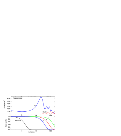
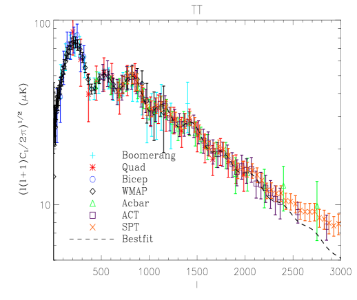
Figure 1: Left-Top: Angular power spectrum for CMB anisotropy (TT) and for EE polarization. The latter has been amplified 20 times to make it visible in the same plot of TT. The angular scale $\gamma$ corresponding to multipole $\ell$ is approximately $\gamma(^{o})=180/\ell$. Left-Bottom: Filter functions of CMB telescopes with different angular resolutions. A FWHM smaller than 1^o is needed to be sensitive to the ”acoustic peaks” due to photon-baryon oscillations in the early universe. The curves are labeled with the beam FWHM. Differential instruments will not be sensitive to multipoles $\ell<180/\alpha(^{o})$ where $\alpha$ is the angular separation of the beam switch; experiments scanning a limited sky region with angular size $\theta$ cannot be sensitive to multipoles with $\ell<180/\theta(^{o})$ . Right: Selected recent measurements of the angular power spectrum of CMB anisotropy.

Our description of fluctuations with respect to the FRW isotropic and homogeneous metric is totally statistical. So we are not able to forecast the map $\Delta T/T$ as a function of $(\theta,\phi)$, but we are able to predict its statistical properties. If the fluctuations are random and Gaussian, all the information encoded in the image is contained in the angular power spectrum of the map, detailing the contributions of the different angular scales to the fluctuations in the map. In other words, the power spectrum of the image of the CMB details the relative abundance of the spots with different angular scales.

If we expand the temperature of the CMB in spherical harmonics, we have

$${\Delta T\over T}=\sum a_{\ell,m}^{T}Y_{\ell}^{m}(\theta,\phi)$$ (2)

the power spectrum of the CMB temperature anisotropy is defined as

$$c_{\ell}^{TT}=\langle TT\rangle=\langle a_{\ell,m}^{T}a_{\ell,m}^{T,*}\rangle$$ (3)

with no dependence on $m$ since there are no preferred directions. Since we have only a statistical description of the observable, the precision with which the theory can be compared to measurement is limited both by experimental errors and by the statistical uncertainty in the theory itself. Each observable has an associated cosmic and sampling variance, which depends on how many independent samples can be observed in the sky. In the case of the $c_{\ell}$s, their distribution is a $\chi^{2}$ with $2\ell+1$ degrees of freedom, which means that low multipoles have a larger intrinsic variance than high multipoles (see e.g. [3]).

Theory predicts the angular power spectrum of CMB anisotropy with remarkable detail, given a model for the generation of density fluctuations in the Universe, and a set of parameters describing the background cosmology. Assuming scale-invariant initial density fluctuations, the main features of the power spectrum $c_{\ell}^{TT}$ are a $1/\left[\ell(\ell+1)\right]$ trend at low multipoles, produced by the Sachs-Wolfe effect[4] (second term in equation 1); a sequence of peaks and dips at multipoles above $\ell=100$, produced by acoustic fluctuations in the primeval plasma of photons and baryons[5, 6, 7], and a damping tail at high multipoles, due to the finite depth of the recombination and free-streaming effects[8]. Detailed models and codes are available to compute the angular power spectrum of the CMB image (see e.g. [9, 10]). The power spectrum $c_{\ell}^{TT}$ derived from the current best-fit cosmological model is plotted in fig.1 (top panel).

High signal-to-noise maps of the CMB have been obtained since year 2000 [11] (see fig.2).

Figure 2: Left: The first map of the CMB with angular resolution and signal to noise ratio sufficient to resolve degree-sized causal horizons in the early universe was obtained by the BOOMERanG experiment, at 145 GHz, using an off-axis telescope flown on a stratospheric balloon[11]. The structures visible in the map are CMB anisotropies, while the contamination from local foregrounds and from instrument noise are both negligible. Right: The WMAP satellite has mapped the whole sky, confirming the ubiquitous presence of causal horizons, and allowing a precise determination of the power spectrum of CMB anisotropy and of the cosmological parameters [12, 13].

From such maps, the power spectrum of CMB anisotropy is now measured quite well (see e.g. [14, 11, 15, 16, 17, 18, 19, 20, 21, 22, 23, 24, 25, 26, 13, 27] and fig.1, right panel); moreover, higher order statistics are now being measured with the accuracy required to constrain cosmological parameters (see e.g. [28]). Despite of the very small signals, the measurements from independent experiments, using diverse experimental techniques, are remarkably consistent. Moreover, an adiabatic inflationary model, with cold dark matter and a cosmological constant, fits very well the measured data (see e.g. [29, 30, 31, 32, 33, 34, 35, 36, 37, 38, 39, 40, 18, 41, 12, 42, 43, 44, 45]).

The CMB is expected to be slightly polarized, since most of the CMB photons undergo a last Thomson scattering at recombination, and the radiation distribution around the scattering centers is slightly anisotropic. Any quadrupole anisotropy in the incoming distribution produces linear polarization in the scattered radiation. The main term of the local anisotropy due to density (scalar) fluctuations is dipole, while the quadrupole term is much smaller. For this reason the expected polarization is quite weak ([46, 47, 48, 49]). The polarization field can be expanded into a curl-free component (E-modes) and a curl component (B-modes). Six auto and cross power spectra can be obtained from these components: $\langle TT\rangle$, $\langle TE\rangle$, $\langle EE\rangle$, $\langle BB\rangle$, $\langle TB\rangle$, and $\langle EB\rangle$. For example

$$c_{\ell}^{TE}=\langle TE\rangle=\langle a_{\ell,m}^{T}a_{\ell,m}^{E,*}\rangle$$ (4)

where the $a_{\ell,m}^{E}$ and $a_{\ell,m}^{B}$ decompose the map of the Stokes parameters $Q$ and $U$ of linear polarization in spin-2 spherical harmonics:

$$(Q\pm iU)(\theta,\phi)=\sum_{\ell m}\left(a_{\ell m}^{E}\mp ia_{\ell m}^{B}\right)~{}_{\pm 2}Y_{\ell m}(\theta,\phi)$$ (5)

.

Due to the parity properties of these components, standard cosmological models have $\langle TB\rangle=0$ and $\langle EB\rangle=0$. Linear scalar (density) perturbations can only produce E-modes of polarization (see e.g. [50]). In the concordance model, $\langle EE\rangle\sim 0.01\langle TT\rangle$, making $\langle EE\rangle$ a very difficult observable to measure. The power spectrum $c_{\ell}^{EE}$ derived from the current best-fit cosmological model is plotted in fig.1 (top-left panel).

Tensor perturbations (gravitational waves) produce both E-modes and B-modes. If inflation happened (see e.g. [51, 52, 53, 54]), it produced a weak background of gravitational waves. The resulting level of the B-modes depends on the energy scale of inflation, but is in general very weak (see e.g. [55, 56]). Alternative scenarios, like the cyclic model[57], do not produce B-modes at all[58].

There is a strong interest in measuring CMB polarization, and in particular the B-modes, because their detection would represent the final confirmation of the inflation hypothesis, and their level would constrain the energy-scale of the inflation process, which, we know, happened at extremely high energies (which cannot be investigated on earth laboratories [59]).

For long time attempts to measure CMB polarization resulted in upper limits (see e.g. [60, 61, 62, 63, 64, 65]). The possibility of detecting the $\langle BB\rangle$ signature of the inflationary gravity waves background renewed the interest in these measurements ([66, 67, 68, 69, 70, 71, 72, 73, 74, 75, 76, 77, 78, 79, 80]). The first statistically significant detections of CMB polarization have been reported by the coherent radiometer experiments DASI[81], CAPMAP[82], CBI[83], WMAP for both $\langle TE\rangle$[77] and $\langle EE\rangle$[84], and by the bolometric instrument BOOMERanG-03[85, 86, 87]. The quality of CMB polarization measurements has improved steadily with the introduction of instruments with detectors arrays, like QUAD[88, 89, 90], BICEP[91], and QUIET[92].

Recent measurements of the angular power spectra of CMB polarization are collected in fig.3. The polarization power spectra measured by these experiments are all consistent with the forecast from the “concordance” model best fitting the WMAP $\langle TT\rangle$ power spectrum. In addition, they constrain the optical depth to reionization (the process ionizing the universe when the first massive stars formed), which is not well constrained by anisotropy measurements alone (see e.g.[93]).

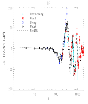
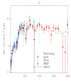
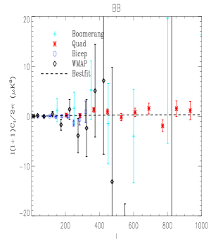
Figure 3: Left: Recent selected measurements of the angular cross-spectrum Temperature-E-modes-polarization $\langle TE\rangle$. Center: Recent selected measurements of the angular power spectrum of E-modes-polarization $\langle EE\rangle$. Right: Recent selected measurements (upper limits) of the angular power spectrum of B-modes-polarization $\langle BB\rangle$. Note the different vertical scales for the three plots. The dashed line is the model prediction for the same cosmological parameters best fitting $\langle TT\rangle$ measurements.

The WMAP data have sufficient coverage to allow a stacking analysis and show the irrotational pattern of polarization pseudovectors around cold and hot spots of the CMB sky[45]: a clear visual demonstration of the polarization produced by density perturbations in the early universe.

To date, measurements of the rotational component of the polarization field $\langle BB\rangle$ resulted in upper limits, implying a ratio of tensor to scalar fluctuations $r\lower 2.15277pt\hbox{$\;\buildrel<\over{\sim}\;$}0.3$.

2 OBSERVING THE CMB

The CMB is a diffuse mm-wave source, filling the sky (with a photon density of $\sim 400\gamma/cm^{3}$) and very faint with respect to radiation produced in the same wavelength range by our living environment and by the instruments used to measure it (the telescope, the optical system, the filters, the detector). The greatest difficulty in measuring the CMB is to reduce the contamination from other sources.

Measuring the specific brightness of the CMB with the COBE-FIRAS instrument required cooling cryogenically the spectrometer (a Martin-Puplett Fourier-Transform Spectrometer) and the bolometric detectors, and launching it in a 400 km orbit. The first operation reduced drastically the emission of the instrument and the noise of the detectors, the second minimized the emission of the earth atmosphere. The COBE-FIRAS was a null-instrument, comparing the specific sky brightness, collected by a multi-mode Winston concentrator[94], to the brightness of an internal cryogenic blackbody reference. The output was precisely nulled (within detector noise) for T_ref=2.725 K . This implies that the brightness of the empty sky is a blackbody at the same temperature, and that the early universe was in thermal equilibrium. The brightness of a 2.725K blackbody[95] is relatively large (compared to the typical noise of mm-wave detectors), but everything at room temperature emits microwaves in the same frequency range: the instrument itself, the surrounding environment, the earth atmosphere. A room-temperature blackbody is orders of magnitude brighter than the CMB. Low emissivity, reflective surfaces must be used to shield the instrument, which needs to be cooled to cryogenic temperatures. Also, to avoid a very wide dynamic range, a cryogenic reference source should be used in the comparison. All this drove the design of the COBE-FIRAS instrument  [1].

The FIRAS one can be considered a definitive measurement of the spectrum of the CMB in the mm range: the deviations from a pure blackbody are less than 0.01% in the peak region, small enough to be fully convincing about the thermal nature of the CMB. However, there are regions of the spectrum where small deviations from a pure blackbody could be expected.

The ARCADE experiment [96, 97], another cryogenic flux collector working with coherent detectors from a stratospheric platform, focused on the low frequency end of the spectrum, looking for cm-wave deviations. In addition to emission from unresolved extragalactic sources, processes like the reionization due to the first stars, and particle decays in the early universe, would heat the diffuse matter, which in turn would cool, injecting the excess heat in the CMB (see e.g. [98]).

CMB anisotropy and polarization measurements target at much smaller brightnesses. The specific brightness of CMB anisotropy (and its polarization) is a modified blackbody

$$\Delta B=B(\nu,T_{CMB})\frac{xe^{x}}{e^{x}-1}\frac{\Delta T}{T}\;\;\;\;;\;\;\;\;x={h\nu\over kT}$$ (6)

peaking at 220 GHz, and with $\Delta T/T$ of the order of 30 ppm, resulting in very faint brightness differences. However, in differential measurements common mode signals (coming from the average CMB but also from the instrument and the environment) can be rejected with high efficiency.

The focus here shifts on angular resolution (i.e. size of the telescope), sensitivity (i.e. noise of the detectors and photon-noise from the radiative background), and mapping speed.

2.1 Angular Resolution and Sidelobes

Theory predicts a power spectrum $c_{\ell}^{**}$ with important features at degree and sub-degree angular scales (i.e. multipoles above $\ell=100$, see top panel of Fig.1). Resolving those features requires sub-degree angular resolution. In the bottom panel of Fig.1 we plot the window function (i.e. the sensitivity of the instrument to different multipoles) for Gaussian beams with different $FWHM$: $B_{\ell}^{2}=e^{-\ell(\ell+1/2)/\sigma^{2}}$, with $\sigma=FWHM/\sqrt{8\ln 2}$ [99].

At the frequency of maximum specific brightness of the CMB (160 GHz), and for a FWHM of 10^′, the diameter of the entrance pupil of a diffraction-limited optical system has to be around 0.8 m. However, to reduce the spillover from strong sources in the sidelobes, it is needed to oversize the entrance pupil (i.e. the diameter of the collecting mirror/lens) leaving a guard-ring around the entrance pupil. The aperture stop is placed in a cold part of the system, effectively apodizing the illumination of primary light collector. So, at least meter-sized telescopes are needed to explore the features of the angular power spectrum of the CMB, while 10m class telescopes are needed to study its finest details.

Bolometric systems are capable of integrating many radiation modes, boosting their sensitivity at the cost of a corresponding increase in the size of the entrance pupil. At lower frequencies, where the atmosphere is more transparent, the required telescope size increases by a large factor (for example by a factor $\sim$ 4 at $\sim$ 40 GHz), entering in the realm of large and expensive telescope structures, including compact interferometric systems.

For all these reasons, CMB telescopes cannot easily be cooled at cryogenic temperatures to reduce their radiative background, unless they are operated in space (see below).

The control of telescope sidelobes is also extremely important. If ground pickup is not properly minimized, the nuisance signal coming from the earth emission in the far sidelobes can be comparable or larger than the CMB anisotropy signal. The detector will receive power from the boresight, pointed to the sky, but also from all the surrounding sources, weighted by the angular response $R$ as follows:

$$W(\theta,\phi)=A\int_{4\pi}B(\theta^{\prime},\phi^{\prime})R(\theta-\theta^{\prime},\phi-\phi^{\prime})d\Omega$$ (7)

where $B(\theta,\phi)$ is the brightness from direction $(\theta,\phi)$.

Beyond the main beam (off-axis angles $\theta\gg\lambda/D$) the envelope of the angular response $R$ for a circular aperture in diffraction limited conditions scales as $\theta^{-3}$. For a ground based experiment, where the sky fills the main beam with solid angle $\Omega_{M}\ll 1$ sr and the emission from ground fills a large solid angle in the sidelobes $\Omega_{S}\sim 2\pi$ sr, the detected signal can be approximated as

$$W\simeq A\left[B_{sky}\langle R\rangle_{M}\Omega_{M}+B_{ground}\langle R\rangle_{S}\Omega_{S}\right]=A\left[I_{M}+I_{S}\right]$$ (8)

where $\langle\rangle_{M,S}$ represent the averages of the angular response $R$ over the main lobe (where $\langle R\rangle_{M}\lower 2.15277pt\hbox{$\;\buildrel<\over{\sim}\;$}1$) and over the sidelobes (where $\langle R\rangle_{S}\ll 1$). In the case of a 2.725K sky emission and of a 250K ground emission, for example, in order to have $I_{S}\ll I_{M}$ we need $\langle R\rangle_{S}\ll 4\times 10^{-5}$ for a 10^o FWHM experiment, and $\langle R\rangle_{S}\ll 1\times 10^{-8}$ for a 10^′ FWHM experiment. Hence the necessity of additional shields surrounding the telescope, to increase the number of diffractions that radiation from the ground must undergo before reaching the detectors.

The situation is even worse in the case of anisotropy measurements, where the interesing signal is of a few $\mu K$. Here a differential instrument is needed, which helps in reducing the sidelobes contribution to the measured signal. The last resource is to send the instrument far from the earth, so that the solid angle occupied by ground emission is $\ll 2\pi$. This is the case for the WMAP and Planck space missions, devoted to CMB anisotropy and polarization measurements. They both operate from the Lagrange point L2 of the sun-earth system, where the solid angle occupied by the earth is only $2\times 10^{-4}$ sr. This relaxes the conditions on sidelobes rejection by a factor $\sim 30000$ with respect to ground-based or balloon-borne experiments.

The telescope and shields configurations are optimized using numerical methods (see e.g. www.ticra.com), normally based on the geometrical theory of diffraction [100] to speed-up the computations (see e.g. [101]).

To reduce the sidelobes, off-axis telescope designs are preferred, and complemented by extensive ground and sun shields (see e.g. [102, 103, 104, 105, 106, 107, 108, 85, 109, 110]). In particular, compact test range telescope configurations offer wide focal planes (allowing the use of large format detector arrays, see below), with excellent cross-polarization quality (which is essential for CMB polarization studies) see e.g. [111, 112].

The actual sidelobes pattern is usually measured with strong far-field sources (like a Gunn oscillator in the focus of a large telescope, producing a plane-wave to illuminate the telescope of the instrument). For space missions, where the operating environment can be very different from the laboratory conditions, the sidelobes are measured during the mission, using the Moon or the Sun (see e.g. [113]).

2.2 Sensitivity

The sensitivity of a detector measuring CMB anisotropy depends on detector performance (usually quantified by its intrinsic noise equivalent temperature, $NET_{i}$, in CMB temperature fluctuation units ($\mu K_{CMB}$)) and on the noise of the incoming radiative background, $NET_{\gamma}$. The latter is computed following [114] (but see also [115, 116]): it depends on the emission of the instrument itself (presence of warm lenses, mirrors, windows) and on the atmosphere above the operation site (the telescope can be ground-based, on a stratospheric balloon, or on a satellite). Operating above the earth atmosphere photon noise is reduced, and the instrument must be cooled cryogenically to exploit the optimal environmental conditions. In figure 4 we compare the photon noise from the natural radiative background and from the instrument to the signal to be detected, for several typical situations. Keep in mind that photon noise $\langle N^{2}\rangle^{1/2}$ in figure 4 is given for unit optical bandwidth (1 $cm^{-1}$), unit electrical bandwidth (1 Hz, roughly corresponding to 1 s of integration), and for a throughput $A\Omega=1cm^{2}sr$, and scales as the square root of these; moreover, in Rayleigh-Jeans conditions, it scales also as the square root of the emissivity $\epsilon$.

Figure 4: Photon noise from the natural radiative background and from the instrument (left scale) compared to CMB anisotropy and polarization signals (right scale). The two top continuous lines represent the noise due to quantum fluctuations of atmospheric emission, for 2 mm PWV and 0.5 mm PWV, typical of a high altitude ground based observatory. The dotted line is the noise due to quantum fluctuations of the emission from the residual atmosphere, at balloon (41 km) altitude. The lower thin continuous line is the photon noise of the CMB itself. The dashed lines represent the noise produced by a low-emissivity ( $\epsilon=5\times 10^{-3}$ ) optical system at different temperatures (300K, 40K, 4K, 1.5K from top to bottom). The dot-dashed lines represent a typical CMB anisotropy brightness fluctuation (corresponding to $\Delta T_{CMB}=90\mu K$, higher line ) and a typical CMB polarization fluctuation (corresponding to $\Delta T_{CMB}=3\mu K$, lower line).

From figure 4 it is evident that ground-based observations are limited to low frequencies ($\;\buildrel<\over{\sim}\;$ 40 GHz) and the W and D bands (note, however, that only quantum fluctuations have been plotted here, while turbulence, winds, instabilities can increase atmospheric noise significantly). Balloon-borne telescopes can work with room-temperature telescopes, while to exploit the low radiative background of space the telescope should be cooled to at least 40K, and better below 4K if high frequency measurements are planned.

Quite recently mm-wave bolometers operated below 0.3K have achieved background limited conditions (i.e. $NET_{i}\lower 2.15277pt\hbox{$\;\buildrel<\over{\sim}\;$}NET_{\gamma}$). This is the case of the bolometers of the HFI instrument[117] aboard of the Planck satellite, where the telescope is cooled radiatively to 40K[118]. For these detectors $NEP_{i}\lower 2.15277pt\hbox{$\;\buildrel<\over{\sim}\;$}10^{-17}W/\sqrt{Hz}$ ([119]), and a cold optical system is required, to exploit their excellent performance (compare this $NEP_{i}$ to the photon noise in fig. 4, for a typical throughput $A\Omega\sim\lambda^{2}\sim 0.05cm^{2}sr$).

2.3 Mapping Speed

Once background-limited conditions are reached, the only way to improve the performance of a CMB survey is to increase the number of detectors simultaneously scanning different directions, i.e. to produce large arrays of mm-wave detectors. This will boost the mapping speed of the experiment, by a factor of the order of the number of detectors in the focal plane. The need for large arrays required an important technology development to achieve fully automated production of a large number of pixels. This is very difficult to achieve in the case of coherent detectors, because of the cost and the power dissipation of each amplifier. In the case of bolometers and other incoherent detectors (like KIDs and CEBs, see below), it has been possible to devise pixel architectures which can be completely produced by photolithography and micromachining, with low cost and negligible power per pixel.

Bolometers are thermal detectors, absorbing radiation and sensing the resulting temperature increase. For a review of CMB bolometers development and operation see e.g. [120, 121]. The development of fully lithographed arrays is the result of a long process started with the development of the so-called spider-web bolometer [122], followed by the polarization sensitive bolometer (PSB) [123]. Several of these devices were arranged on the same wafer [124]. Then voltage-biased Transition Edge superconducting Sensors (TES) were developed (see e.g. [125, 126, 127, 128, 129] and integrated on the array wafer (see e.g. [130, 131, 132, 133, 134, 135, 136, 137]). In parallel to the development of the TES bolometers, a large effort has been spent in the development of the readout electronics, which uses SQUIDs to read and multiplex a large number of detectors with a limited number of wires, thus maintaining the heat load on the cryostat at manageable levels [138, 139]. These detectors have been installed at large CMB telescopes (ACT, SPT, APEX …) with excellent performance, providing high resolution CMB measurements. Antenna coupling to the radiation, dual polarization sensitivity, and even spectral filtering are now also integrated in the TES wafers (see e.g.[140, 141, 142, 143, 144, 145, 146]), producing powerful imaging/polarimetry/spectrometry capabilities in a lightweight block.

In addition to TESs, the quest for large mm-wave cameras for CMB research drove the development of other non-coherent detection technologies.

In the MKIDs (microwave kinetic inductance detectors) low energy photons (like CMB photons, in the meV range) break Cooper pairs in a superconducting film, changing its surface impedance, and in particular the kinetic inductance $L_{k}$. The change is small, but can be measured using the film as the inductor in a superconducting resonator, which can have very high merit factor $Q$, up to $\simeq 10^{6}$, and thus be very sensitive to the variations of its components. Many independent MKIDs are arranged in an array, an shunt the same line, where a comb of frequencies fitting the resonances of the pixels is carried. CMB photons absorbed by a given pixel produce a change in the transmission of a single frequency of the comb. So MKIDs are intrinsically multiplexable, requiring only two shielded cables to supply and read hundreds of pixels. The initial KID concept [147], where mm-wave photons are antenna coupled to the resonator, has evolved in the LEKID (Lumped Elements Kinetic Inductance Detector) concept [148, 149], where the resonator is shaped as an efficient absorber of mm-waves analogous to bolometer absorbers. The great advantage of MKIDs with respect to TES is that the fabrication process is significantly simpler, and also the readout electronics requires only a wide-band amplifier cryogenically cooled. Today, MKID arrays are produced in many laboratories (see e.g. [150, 151, 152]) and are starting to be operated at large telescopes (see e.g. [153, 154]).

In a Cold Electron Bolometer (CEB) [155] the signal power collected by an antenna is capacitively coupled to a tunnel-junction (SIN) sensor and is dissipated in the electrons which act as a nanoabsorber; it is also removed from the absorber in the form of hot electrons by the same SIN junctions. This electron cooling provides strong negative electrothermal feedback, improving the time-constant, the responsivity and the NEP[156]. Since the thermistor is the gas of electrons, confined in a $\sim$ 100 nm junction and thermally insulated from the rest of the sensor, these detectors should be quite immune to cosmic-rays hits, an important nuisance for TES and KIDs in space. Moreover, these detectors promise very good performance in a wide range of radiative backgrounds, while efficient multiplexing schemes are still to be developed.

3 CURRENT TRENDS IN CMB RESEARCH

We have entered the era of precision observations of the CMB.

Planck [157] has produced a shallow survey of the whole sky in nine mm - submm bands (centered at 30, 44, 70, 100, 143, 217, 353, 545, 857 GHz). Taking advantage of the wide frequency coverage and of the extreme sensitivity of the measurements, it is possible to separate efficiently the different contributions to the brightness of the sky along each line of sight (see figure 5).

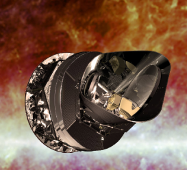
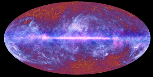
Figure 5: Left: The Planck satellite, scanning the sky in the mm/submm from the Lagrangian point L2 of the sun-earth system. Right: Map of the sky in Galactic coordinates, obtained from the full sky surveys of Planck at nine frequencies. The maps have been linearly combined in two ways: the red-yellow palette evident at high galactic latitudes is the combination maximizing CMB signals. Here the horizon-sized spots are ubiquitous and dominant at high galactic latitudes. The blue-white palette is the combination maximizing the local foreground. The power of wide frequency coverage is evident: from this map it is possible to monitor the faintest interstellar clouds at high galactic latitudes. Figure credit: European Space Agency.

While it is evident from fig.5 that foreground emission can be important even at high galactic latitudes, it is also clear that the multifrequency survey of Planck allows to detect and remove tiny contaminations from thin interstellar clouds. With the foregrounds under control, Planck is expected to produce very precise measurements of CMB anisotropy and polarization in the next data release, early in 2013.

High-resolution anisotropy measurements are now performed mainly in the direction of clusters of galaxies (SZ effect) and to search for non-Gaussianity of the CMB. High sensitivity polarization measurements aim at measuring B-modes from inflation and from lensing of E-modes. We will outline here a few, selected issues that we consider relevant for the continuation of these studies.

3.1 Sunyaev-Zeldovich Effect and spectral anisotropy measurements

The Sunyaev-Zeld́ovich (SZ) effect[158] is the energization of CMB photons crossing clusters of galaxies, due to the inverse Compton effect with the hot intergalactic plasma. The order of magnitude of the effect can be estimated noticing that the optical depth for a rich cluster is $\tau\sim n_{e}\sigma_{T}\ell\lower 2.15277pt\hbox{$\;\buildrel<\over{\sim}\;$}0.01$ and the fractional energy gain of each interacting photon is of the order of $kT_{e}/m_{e}c^{2}\sim 0.01$, so the fractional CMB temperature change will be $\Delta T/T\sim\tau kT_{e}/m_{e}c^{2}\lower 2.15277pt\hbox{$\;\buildrel<\over{\sim}\;$}10^{-4}$: a large signal if compared to the primordial CMB anisotropy. The SZ effect is thus a powerful tool for studying the physics of clusters and using them as cosmological probes (see e.g. [159, 160, 161]). Large mm-wave telescopes ([109, 110, 136]), coupled to imaging multi-band arrays of bolometers, are now operating in excellent sites and produce a number of detections and maps of the SZ effect in selected sky areas, discovering new clusters, and establishing cluster and cosmological parameters.

From the Planck data an early catalogue of massive clusters detected via the SZ effect has been extracted[162]. This consists of 169 known clusters, plus 20 new discoveries, including exceptional members[163]. All these measurements take advantage of the extreme sensitivity of bolometers, with their excellent performance in the frequency range 90-600 GHz where the spectral signatures of the SZ effect lie.

Several components contribute to the signal detected from the line of sight crossing the cluster: a thermal component due to the inverse Compton effect; a Doppler component, caused by the collective motion of the cluster with respect to the CMB restframe; a non-thermal component caused by a non-thermal population of electrons, produced by e.g. the AGNs present in the cluster, relativistic plasma in cluster cavities, shock acceleration; the intrinsic anisotropy of the CMB; the emission of dust, free-free and synchrotron in our Galaxy and in the galaxies of the cluster. Since the spectrum of thermal SZ significantly departs from the spectra of the foreground and background components, multi-frequency SZ measurements allow the estimation of several physical parameters of the cluster, provided there are more observation bands than parameters to be determined, or some of the contributions are known to be negligible. In [164] we have analyzed how different experimental configurations perform in this particular components separation exercise. Ground-based few-band photometers cannot provide enough information to separate all physical components, because atmospheric noise limits the number of useful independent bands. These instruments need external information (optical, X-ray, far-IR, etc.) to produce mainly measurements of the optical depth of the thermal SZ (see e.g. [165, 166, 167, 168, 169, 170, 171, 172]).

Future space-based spectrometers can cover the full range of interesting frequencies and offer much more information. A cryogenic differential imaging Fourier Transform Spectrometer (FTS) in the focal plane of a space mission with a cold telescope, like Millimetron[173], would be a powerful experiment, measuring accurately all the parameters of a cluster. The FIRAS experiment has demonstrated the power of these large-throughput, wide frequency coverage instruments, which are intrinsically differential. In that case one of the two input ports collected radiation from the sky, while the other port was illuminated by an internal blackbody: the perfect nulling of the measured difference spectrum demonstrated accurately the blackbody nature of the cosmic microwave background. In this implementation, the two input ports of the instrument collect radiation from two contiguous regions of the focal plane of the same telescope (see left panel of fig.6). In this way only the anisotropic component of the brightness distribution produces a measurable signal, while the common-mode signals from the instrument, the telescope, and the CMB itself are efficiently rejected. The FTS is sensitive to a wide frequency band (say 70 - 1000 GHz for SZ studies), so photon noise is the limiting factor. In fig.6 we compare what can be achieved with a warm system on a stratospheric balloon[174, 175, 176] (center panel) to what can be ultimately achieved with a cold system in deep space[164] (right panel). In both cases important improvements with respect to the state-of-the-art determination of cluster parameters are expected. The intermediate case of a cold spectrometer coupled to a warm telescope in a Molniya orbit has been studied in [177] .

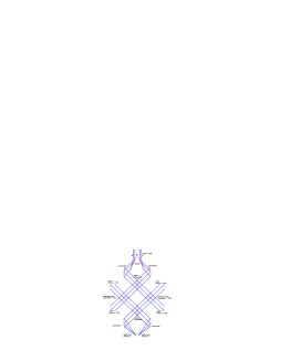
Figure 6: Left : Block-diagram of a differential FTS. This very symmetrical configuration reduces instrumental offsets and doubles the efficiency with respect to the standard MPI FTS[178]. Center : Simulated observations of a rich cluster of galaxies with a warm differential FTS aboard of a stratospheric balloon, like OLIMPO. Right : Same for a differential FTS aboard of a satellite in L2, with a large (10m) cold (4K) telescope, like Millimetron. In both cases, 3 hours of observation are assumed, and bolometer performance limited only by the radiative background. The two continuous lines represent the SZ effect from the plasma in the cluster and differential emission of interstellar dust, the two main components of the measured brightness.

Other important scientific targets of these instruments are the measurement of the $C^{+}$ and CO lines, in the redshift desert and beyond, for a large number of galaxies, and spectral observations of a number of processes in the early universe and in the recombination and reionization eras (see e.g. [179, 180, 181, 177, 182, 183]).

3.2 B-modes of CMB polarization

Measuring the tiny B-modes signal is a formidable experimental challenge. For this reason it is very important that independent teams develop advanced experiments, using different techniques and methods. Only independent consistent detections will provide convincing evidence for the existence of B-modes.

The mainstream in this field is the use of large arrays of single-mode bolometric polarimeters, using a polarization modulator in the optical path (as close as possible to the input port of the instrument, to avoid modulating instrumental polarization) to modulate only the polarized part of the incoming signal. The throughput of the telescope has to be very large, of the order of $\sum_{i=1}^{n}N_{i}\lambda_{i}^{2}/F_{i}$, where the number of detectors $N_{i}$ in each band $i$ is of the order of 10³, and the filling factor of the focal plane is $F_{i}\lower 2.15277pt\hbox{$\;\buildrel<\over{\sim}\;$}1$.

The removal of the polarized foreground (mainly produced by the interstellar medium) is a matter of the utmost importance. It has been analyzed in great detail, most recently in the framework of the Planck mission (see e.g. [184, 185, 186] and references therein) and of future missions devoted to CMB polarization (see e.g. [187]). The solution is to carry out surveys with wide frequency coverage, from tens of GHz (to survey strongly polarized synchrotron emission) to several hundreds of GHz (to survey polarized emission from interstellar dust). For this reason a number of bands $n\sim 10$ is required to separate the foreground components from the primordial CMB signal. Accommodating all the bands in the focal plane of the telescope exacerbates the large throughput problem for these systems, also because only the center region of the focal plane has optimal polarization efficiency and beam-symmetry properties. Multichroic pixels including bolometric detectors in 3 or more bands under the same microlens have been developed [146], allowing a very efficient use of focal plane space. This approach has been proposed for the LiteBIRD satellite [188].

In the case of incoherent detectors, intrinsically insensitive to the polarization status of the incoming power, the classic Stokes polarimeter requires a half-wave plate retarder plus a polarizer. If the HWP is rotated with a rotation rate ${\dot{\theta}}$, the linearly polarized part of the incoming signal is modulated at $4{\dot{\theta}}$, while the unpolarized and the circular polarization components are not modulated. Wide-band retarders can be obtained in transmission using a sandwich of birefringent crystals (see e.g. [189, 190, 191, 192, 193]) or suitable meta-materials assembled with metal meshes [194]. In reflection, a rotation mirror / polarizer combination [195] can be used, or a translating polarizer / mirror assembly (Variable Delay Modulator [196]), or a translating circular polarizer / mirror combination (Transational Polarization Rotator [197]). The main issues with these modulators is the equalization of the transmission (reflection) for the two orthogonal polarizations (any mismatch, even at a level of 1$\%$, will produce a comparatively very large $2{\dot{\theta}}$ signal) and the need to cool at cryogenic temperatures the modulator, to reduce its (polarized) emission (see [198] for a discussion).

Reaching satisfactory performance over a wide frequency band and a wide throughput is problematic. In the case of the dielectric HWP, a sandwich of differently oriented plates is required, following the Pancharatman [199] recipe. This approach is suitable for accurate measurements of CMB polarization in the range 120-450 GHz[200]. However, it is currently impossible to obtain large-diameter ($\lower 2.15277pt\hbox{$\;\buildrel>\over{\sim}\;$}30cm$) slabs of sapphire (or any other birefringent crystal suitable for mm wavelengths), so their use is limited to medium throughput systems. Using metal meshes might solve the problem, but requires a careful equalization of the conductivity of the meshes. In the case of the mirror/polarizer combination, which can be produced in very large sizes, the operative band is restricted to $\sim 20\%$ of the center frequency. It is possible, however, to operate the modulator at multiples of a fundamental frequency, with decreasing fractional bandwidth, as proposed in [201].

A Martin-Puplett Fourier Transform Spectrometer[178], with the two input ports $A$ and $B$ (fig.6) co-aligned to look at the same sky patch, becomes a polarimeter. In fact, it produces at the two output ports $a$ and $b$, with polarization $x$ and $y$, the following 4 signals, which can be detected by 4 independent detectors: $[I_{a,x}(z)-\langle I_{a,x}\rangle]\propto\int(E^{2}_{B,x}(\sigma)-E^{2}_{A,y}(\sigma))cos(4\pi\sigma z)d\sigma$ ; $[I_{a,y}(z)-\langle I_{a,y}\rangle]\propto\int(E^{2}_{B,y}(\sigma)-E^{2}_{A,x}(\sigma))cos(4\pi\sigma z)d\sigma$ ; $[I_{b,x}(z)-\langle I_{b,x}\rangle]\propto\int(E^{2}_{A,x}(\sigma)-E^{2}_{B,y}(\sigma))cos(4\pi\sigma z)d\sigma$ ; $[I_{b,y}(z)-\langle I_{b,y}\rangle]\propto\int(E^{2}_{A,y}(\sigma)-E^{2}_{B,x}(\sigma))cos(4\pi\sigma z)d\sigma$ , where $\sigma$ is the wavenumber and $z$ is the position of the moving mirror. Summing and subtracting the Fourier-transformed signals from detectors couples it is possible to estimate the $\sl frequency$ $\sl spectra$ of the Stokes parameters of the incoming radiation. This is the principle of operation of the proposed PIXIE experiment[182], a space-based large-throughput spectro-polarimeter covering the frequency range 30-6000 GHz. The optical axis of the spectro-polarimeter is aligned to the spin axis of the satellite, so that any polarization signal becomes spin-synchronous. In this configuration, the specifications for beam ellipticity, and beam, gain and polarization mismatch for the four detectors are very stringent. These could be relaxed with the use of a rotating achromatic HWP at the entrance of the system, but it is currently impossible to fabricate a high-efficiency highly-balanced HWP over such a wide frequency range.

There is a long list of potential systematic effects in Stokes polarimeters (see e.g. [202]), and the requirements for a clean detection of B-modes are extremely stringent (see e.g. table 6.1 in [203]). A few examples: tens of mK signals at $2{\dot{\theta}}$ are produced by the unpolarized 2.7K background, modulated by $\sim 1\%$ efficiency mismatch between the ordinary and extraordinary rays in the waveplate. The emission of a mismatched HWP also produces tens of mK signals at $2{\dot{\theta}}$, unless its temperature is below 2K. These signals challenge the dynamic range of the detector, which is optimized for measuring CMB polarization signals $\sim 10^{4}$ times smaller. Any non-linearity in the detector can convert part of this $2{\dot{\theta}}$ signal into a $4{\dot{\theta}}$ signal, producing a large offset in the polarization measurement. If part of the emission of the polarizer is reflected back by the waveplate, it is modulated at $4{\dot{\theta}}$, contributing with additional $\sim$ few $\mu K$ signals to the offset. A possible solution to this problem is the step and integrate strategy (see e.g. [204]). At variance with the continuous rotation strategy, here the HWP is kept steady during sky scans, and angular steps are performed at the turnarounds. All the systematic effects generated internally to the instrument produce a constant offset during each scan, which can be removed, while the sky polarization is modulated at the (very low) frequency of the repetition of the scans. In addition to these effect, other noticeable sources of systematic problems are the ellipticity of the main beam ($<10^{-4}$), the level of its polarized sidelobes ($<10^{-6}$), the instrumental polarization ($<10^{-4}$), the relative gain calibration ($<10^{-5}$): all these convert unpolarized brightness fluctuations into apparent B-modes signals; an error in the main polarimeter axis angle ($<0.2^{o}$) and the cross-polar response ($<3\times 10^{-3}$) convert E-modes into apparent B-modes; moreover, the relative pointing of differenced observation directions must be $<0.1$ arcsec to avoid conversion of brightness fluctuations into apparent B-mode signals. Pathfinder experiments are the best way to find and test the best mitigation methods for all these subtle systematic effects. Current attempts exploit different techniques, ranging from ground-based coherent polarimeters, like QUIET[92], to ground-based bolometer arrays with HWP, like POLARBEAR[205], to ground-based bolometric interferometers, like QUBIC[206], to stratospheric balloons like SPIDER[207], EBEX[208], and LSPE[209]. Using completely independent techniques, these experiments provide a powerful test set for any detection of B-modes in the CMB, in view of a post-Planck next generation space mission for the CMB.

4 CONCLUSIONS

The future of CMB studies is bright. A large community has grown around the success of CMB missions, producing large amounts of excellent data. The experiments have drifted from a situation where sensitivity was the issue to a situation where control of systematic effects is the main problem. So we are facing very difficult challenges, with the ambition of understanding the most distant phenomena happening in our universe, analyzing tiny signals embedded in an overwhelming noisy background. When we approached CMB research for the first time, in 1980, measuring the intrinsic anisotropy of the CMB was considered almost science-fiction. Today CMB anisotropy is measured in a single pass with scanning telescopes using large arrays of bolometers. This experience makes us confident that much more is coming in this field, with the enthusiastic contribution of young researchers and the cross-fertilization between cosmologists, astrophysicists, solid-state / detector physicists, optics experts.

- [1] Mather, J. C., Fixsen, D. J., and Shafer, R. A., e. a., “Calibrator Design for the COBE Far-Infrared Absolute Spectrophotometer (FIRAS),” ApJ 512, 511–520 (Feb. 1999).
- [2] Padmanabhan, T., [Structure Formation in the Universe ] (June 1993).
- [3] White, M., Krauss, L. M., and Silk, J., “Cosmic Variance in Cosmic Microwave Background Anisotropies: From 1 degrees to COBE,” ApJ 418, 535 (Dec. 1993).
- [4] Sachs, R. K. and Wolfe, A. M., “Perturbations of a Cosmological Model and Angular Variations of the Microwave Background,” ApJ 147, 73 (Jan. 1967).
- [5] Sunyaev, R. A. and Zeldovich, Y. B., “Small-Scale Fluctuations of Relic Radiation,” Ap&SS 7, 3–19 (Apr. 1970).
- [6] Peebles, P. J. E. and Yu, J. T., “Primeval Adiabatic Perturbation in an Expanding Universe,” ApJ 162, 815 (Dec. 1970).
- [7] Hu, W. and White, M., “Acoustic Signatures in the Cosmic Microwave Background,” ApJ 471, 30 (Nov. 1996).
- [8] Hu, W. and White, M., “The Damping Tail of Cosmic Microwave Background Anisotropies,” ApJ 479, 568 (Apr. 1997).
- [9] Hu, W. and Dodelson, S., “Cosmic Microwave Background Anisotropies,” ARA&A 40, 171–216 (2002).
- [10] Lewis, A., Challinor, A., and Lasenby, A., “Efficient Computation of Cosmic Microwave Background Anisotropies in Closed Friedmann-Robertson-Walker Models,” ApJ 538, 473–476 (Aug. 2000).
- [11] de Bernardis, P., Ade, P. A. R., and Bock, J. J. e. a., “A flat Universe from high-resolution maps of the cosmic microwave background radiation,” Nature 404, 955–959 (Apr. 2000).
- [12] Bennett, C. L., Hill, R. S., and Hinshaw, G. e. a., “First-Year Wilkinson Microwave Anisotropy Probe (WMAP) Observations: Foreground Emission,” ApJS 148, 97–117 (Sept. 2003).
- [13] Larson, D., Dunkley, J., and Hinshaw, G. e. a., “Seven-year Wilkinson Microwave Anisotropy Probe (WMAP) Observations: Power Spectra and WMAP-derived Parameters,” ApJS 192, 16 (Feb. 2011).
- [14] Wright, E. L., Mather, J. C., and Bennett, C. L. e. a., “Preliminary spectral observations of the Galaxy with a 7 deg beam by the Cosmic Background Explorer (COBE),” ApJ 381, 200–209 (Nov. 1991).
- [15] Lee, A. T., Ade, P., and Balbi, A. e. a., “A High Spatial Resolution Analysis of the MAXIMA-1 Cosmic Microwave Background Anisotropy Data,” ApJ 561, L1–L5 (Nov. 2001).
- [16] de Bernardis, P., Ade, P. A. R., and Bock, J. J. e. a., “Multiple Peaks in the Angular Power Spectrum of the Cosmic Microwave Background: Significance and Consequences for Cosmology,” ApJ 564, 559–566 (Jan. 2002).
- [17] Halverson, N. W., Leitch, E. M., and Pryke, C. e. a., “Degree Angular Scale Interferometer First Results: A Measurement of the Cosmic Microwave Background Angular Power Spectrum,” ApJ 568, 38–45 (Mar. 2002).
- [18] Ruhl, J. E., Ade, P. A. R., and Bock, J. J. e. a., “Improved Measurement of the Angular Power Spectrum of Temperature Anisotropy in the Cosmic Microwave Background from Two New Analyses of BOOMERANG Observations,” ApJ 599, 786–805 (Dec. 2003).
- [19] Grainge, K., Carreira, P., and Cleary, K. e. a., “The cosmic microwave background power spectrum out to l= 1400 measured by the Very Small Array,” MNRAS 341, L23–L28 (June 2003).
- [20] Jones, W. C., Ade, P. A. R., and Bock, J. J. e. a., “A Measurement of the Angular Power Spectrum of the CMB Temperature Anisotropy from the 2003 Flight of BOOMERANG,” ApJ 647, 823–832 (Aug. 2006).
- [21] Kuo, C. L., Ade, P. A. R., and Bock, J. J. e. a., “Improved Measurements of the CMB Power Spectrum with ACBAR,” ApJ 664, 687–701 (Aug. 2007).
- [22] Hinshaw, G., Spergel, D. N., and Verde, L. e. a., “First-Year Wilkinson Microwave Anisotropy Probe (WMAP) Observations: The Angular Power Spectrum,” ApJS 148, 135–159 (Sept. 2003).
- [23] Hinshaw, G., Nolta, M. R., and Bennett, C. L. e. a., “Three-Year Wilkinson Microwave Anisotropy Probe (WMAP) Observations: Temperature Analysis,” ApJS 170, 288–334 (June 2007).
- [24] Nolta, M. R., Dunkley, J., and Hill, R. S. e. a., “Five-Year Wilkinson Microwave Anisotropy Probe Observations: Angular Power Spectra,” ApJS 180, 296–305 (Feb. 2009).
- [25] Reichardt, C. L., Ade, P. A. R., and Bock, J. J. e. a., “High-Resolution CMB Power Spectrum from the Complete ACBAR Data Set,” ApJ 694, 1200–1219 (Apr. 2009).
- [26] Fowler, J. W., Acquaviva, V., and Ade, P. A. R. e. a., “The Atacama Cosmology Telescope: A Measurement of the 600 8000 Cosmic Microwave Background Power Spectrum at 148 GHz,” ApJ 722, 1148–1161 (Oct. 2010).
- [27] Das, S., Marriage, T. A., and Ade, P. A. R. e. a., “The Atacama Cosmology Telescope: A Measurement of the Cosmic Microwave Background Power Spectrum at 148 and 218 GHz from the 2008 Southern Survey,” ApJ 729, 62 (Mar. 2011).
- [28] Das, S., Sherwin, B. D., and Aguirre, P. e. a., “Detection of the Power Spectrum of Cosmic Microwave Background Lensing by the Atacama Cosmology Telescope,” Physical Review Letters 107, 021301 (July 2011).
- [29] de Bernardis, P., de Gasperis, G., and Masi, S. e. a., “Detection of cosmic microwave background anisotropy at 1.8 deg: Theoretical implications on inflationary models,” ApJ 433, L1–L4 (Sept. 1994).
- [30] Bond, J. R., Jaffe, A. H., and Knox, L., “Estimating the power spectrum of the cosmic microwave background,” Phys. Rev. D 57, 2117–2137 (Feb. 1998).
- [31] Bond, J. R., Jaffe, A. H., and Knox, L., “Radical Compression of Cosmic Microwave Background Data,” ApJ 533, 19–37 (Apr. 2000).
- [32] Dodelson, S. and Knox, L., “Dark Energy and the Cosmic Microwave Background Radiation,” Physical Review Letters 84, 3523–3526 (Apr. 2000).
- [33] Tegmark, M. and Zaldarriaga, M., “Current Cosmological Constraints from a 10 Parameter Cosmic Microwave Background Analysis,” ApJ 544, 30–42 (Nov. 2000).
- [34] Tegmark, M. and Zaldarriaga, M., “New Microwave Background Constraints on the Cosmic Matter Budget: Trouble for Nucleosynthesis?,” Physical Review Letters 85, 2240–2243 (Sept. 2000).
- [35] Bridle, S. L., Zehavi, I., and Dekel, A. e. a., “Cosmological parameters from velocities, cosmic microwave background and supernovae,” MNRAS 321, 333–340 (Feb. 2001).
- [36] Douspis, M., Bartlett, J. G., and Blanchard, A. e. a., “Concerning parameter estimation using the cosmic microwave background,” A&A 368, 1–14 (Mar. 2001).
- [37] Lange, A. E., Ade, P. A., and Bock, J. J. e. a., “Cosmological parameters from the first results of Boomerang,” Phys. Rev. D 63, 042001 (Feb. 2001).
- [38] Jaffe, A. H., Ade, P. A., and Balbi, A. e. a., “Cosmology from MAXIMA-1, BOOMERANG, and COBE DMR Cosmic Microwave Background Observations,” Physical Review Letters 86, 3475–3479 (Apr. 2001).
- [39] Lewis, A. and Bridle, S., “Cosmological parameters from CMB and other data: A Monte Carlo approach,” Phys. Rev. D 66, 103511 (Nov. 2002).
- [40] Netterfield, C. B., Ade, P. A. R., and Bock, J. J. e. a., “A Measurement by BOOMERANG of Multiple Peaks in the Angular Power Spectrum of the Cosmic Microwave Background,” ApJ 571, 604–614 (June 2002).
- [41] Spergel, D. N., Verde, L., and Peiris, H. V. e. a., “First-Year Wilkinson Microwave Anisotropy Probe (WMAP) Observations: Determination of Cosmological Parameters,” ApJS 148, 175–194 (Sept. 2003).
- [42] Tegmark, M., Strauss, M. A., and Blanton, M. R. e. a., “Cosmological parameters from SDSS and WMAP,” Phys. Rev. D 69, 103501 (May 2004).
- [43] Spergel, D. N., Bean, R., and Doré, e. a., “Three-Year Wilkinson Microwave Anisotropy Probe (WMAP) Observations: Implications for Cosmology,” ApJS 170, 377–408 (June 2007).
- [44] Komatsu, E., Dunkley, J., and Nolta, M. R. e. a., “Five-Year Wilkinson Microwave Anisotropy Probe Observations: Cosmological Interpretation,” ApJS 180, 330–376 (Feb. 2009).
- [45] Komatsu, E., Smith, K. M., and Dunkley, J. e. a., “Seven-year Wilkinson Microwave Anisotropy Probe (WMAP) Observations: Cosmological Interpretation,” ApJS 192, 18 (Feb. 2011).
- [46] Rees, M. J., “Polarization and Spectrum of the Primeval Radiation in an Anisotropic Universe,” ApJ 153, L1 (July 1968).
- [47] Kaiser, N., “Small-angle anisotropy of the microwave background radiation in the adiabatic theory,” MNRAS 202, 1169–1180 (Mar. 1983).
- [48] Hu, W. and White, M., “A CMB polarization primer,” New A 2, 323–344 (Oct. 1997).
- [49] Kamionkowski, M., Kosowsky, A., and Stebbins, A., “Statistics of cosmic microwave background polarization,” Phys. Rev. D 55, 7368–7388 (June 1997).
- [50] Seljak, U., Pen, U.-L., and Turok, N., “Polarization of the Microwave Background in Defect Models,” Physical Review Letters 79, 1615–1618 (Sept. 1997).
- [51] Mukhanov, V. F. and Chibisov, G. V., “Quantum fluctuations and a nonsingular universe,” ZhETF Pis ma Redaktsiiu 33, 549–553 (May 1981).
- [52] Guth, A. H. and Pi, S.-Y., “Fluctuations in the new inflationary universe,” Physical Review Letters 49, 1110–1113 (Oct. 1982).
- [53] Linde, A. D., “Chaotic inflation,” Physics Letters B 129, 177–181 (Sept. 1983).
- [54] Kolb, E. W. and Turner, M. S., [The early universe. ] (1990).
- [55] Copeland, E. J., Kolb, E. W., and Liddle, A. R. e. a., “Observing the inflation potential,” Physical Review Letters 71, 219–222 (July 1993).
- [56] Turner, M. S., “Recovering the inflationary potential,” Phys. Rev. D 48, 5539–5545 (Dec. 1993).
- [57] Steinhardt, P. J. and Turok, N., “A Cyclic Model of the Universe,” Science 296, 1436–1439 (May 2002).
- [58] Boyle, L. A., Steinhardt, P. J., and Turok, N., “New duality relating density perturbations in expanding and contracting Friedmann cosmologies,” Phys. Rev. D 70, 023504 (July 2004).
- [59] Liddle, A. R., “The inflationary energy scale,” Phys. Rev. D 49, 739–747 (Jan. 1994).
- [60] Caderni, N., Fabbri, R., and Melchiorri, B. e. a., “Polarization of the microwave background radiation. II. An infrared survey of the sky,” Phys. Rev. D 17, 1908–1918 (Apr. 1978).
- [61] Nanos, Jr., G. P., “Polarization of the blackbody radiation at 3.2 centimeters,” ApJ 232, 341–347 (Sept. 1979).
- [62] Lubin, P. M. and Smoot, G. F., “Polarization of the cosmic background radiation,” ApJ 245, 1–17 (Apr. 1981).
- [63] Masi, S., “Search for the Cosmic Background Polarization,” in [Gamow Cosmology ], 310 (1986).
- [64] Partridge, R. B., Nowakowski, J., and Martin, H. M., “Linear polarized fluctuations in the cosmic microwave background,” Nature 331, 146 (Jan. 1988).
- [65] Wollack, E. J., Devlin, M. J., and Jarosik, N. e. a., “An Instrument for Investigation of the Cosmic Microwave Background Radiation at Intermediate Angular Scales,” ApJ 476, 440 (Feb. 1997).
- [66] Keating, B. G., O’Dell, C. W., and de Oliveira-Costa, A. e. a., “A Limit on the Large Angular Scale Polarization of the Cosmic Microwave Background,” ApJ 560, L1–L4 (Oct. 2001).
- [67] Subrahmanyan, R., Kesteven, M. J., and Ekers, R. D. e. a., “An Australia Telescope survey for CMB anisotropies,” MNRAS 315, 808–822 (July 2000).
- [68] Hedman, M. M., Barkats, D., and Gundersen, J. O. e. a., “New Limits on the Polarized Anisotropy of the Cosmic Microwave Background at Subdegree Angular Scales,” ApJ 573, L73–L76 (July 2002).
- [69] Piccirillo, L., Ade, P. A. R., and Bock, J. J., e. a., “QUEST-A 2.6-m mm-wave telescope for CMB polarization studies,” in [Astrophysical Polarized Backgrounds ], Cecchini, S., Cortiglioni, S., Sault, R., and Sbarra, C., eds., American Institute of Physics Conference Series 609, 159–163 (Mar. 2002).
- [70] Delabrouille, J. and Kaplan, J., “Measuring CMB polarization with the Planck HFI,” in [Astrophysical Polarized Backgrounds ], Cecchini, S., Cortiglioni, S., Sault, R., and Sbarra, C., eds., American Institute of Physics Conference Series 609, 135–143 (Mar. 2002).
- [71] Masi, S., de Bernardis, P., and de Troia, G. e. a., “Scanning polarimeters for measurements of CMB polarization,” in [Experimental Cosmology at Millimetre Wavelengths ], de Petris, M. and Gervasi, M., eds., American Institute of Physics Conference Series 616, 168–174 (May 2002).
- [72] Villa, F., Mandolesi, N., and Bersanelli, M. e. a., “The low frequency instrument of the Planck mission,” in [Astrophysical Polarized Backgrounds ], Cecchini, S., Cortiglioni, S., Sault, R., and Sbarra, C., eds., American Institute of Physics Conference Series 609, 144–149 (Mar. 2002).
- [73] Kovac, J. M., Leitch, E. M., and Pryke, C. e. a., “Detection of polarization in the cosmic microwave background using DASI,” Nature 420, 772–787 (Dec. 2002).
- [74] Johnson, B. R., Abroe, M. E., and Ade, P. e. a., “MAXIPOL: a balloon-borne experiment for measuring the polarization anisotropy of the cosmic microwave background radiation,” New A Rev. 47, 1067–1075 (Dec. 2003).
- [75] Keating, B. G., Ade, P. A. R., and Bock, J. J. e. a., “BICEP: a large angular scale CMB polarimeter,” in [Society of Photo-Optical Instrumentation Engineers (SPIE) Conference Series ], Fineschi, S., ed., Society of Photo-Optical Instrumentation Engineers (SPIE) Conference Series 4843, 284–295 (Feb. 2003).
- [76] Keating, B. G., O’Dell, C. W., and Gundersen, J. O. e. a., “An Instrument for Investigating the Large Angular Scale Polarization of the Cosmic Microwave Background,” ApJS 144, 1–20 (Jan. 2003).
- [77] Kogut, A., Spergel, D. N., and Barnes, C. e. a., “First-Year Wilkinson Microwave Anisotropy Probe (WMAP) Observations: Temperature-Polarization Correlation,” ApJS 148, 161–173 (Sept. 2003).
- [78] Farese, P. C., Dall’Oglio, G., and Gundersen, e. a., “COMPASS: An Upper Limit on Cosmic Microwave Background Polarization at an Angular Scale of 20’,” ApJ 610, 625–634 (Aug. 2004).
- [79] Cortiglioni, S., Bernardi, G., and Carretti, E. e. a., “The Sky Polarization Observatory,” New A 9, 297–327 (May 2004).
- [80] Cartwright, J. K., Pearson, T. J., and Readhead, A. C. S. e. a., “Limits on the Polarization of the Cosmic Microwave Background Radiation at Multipoles up to l ~ 2000,” ApJ 623, 11–16 (Apr. 2005).
- [81] Leitch, E. M., Kovac, J. M., and Halverson, N. W. e. a., “Degree Angular Scale Interferometer 3 Year Cosmic Microwave Background Polarization Results,” ApJ 624, 10–20 (May 2005).
- [82] Barkats, D., Bischoff, C., and Farese, e. a., “First Measurements of the Polarization of the Cosmic Microwave Background Radiation at Small Angular Scales from CAPMAP,” ApJ 619, L127–L130 (Feb. 2005).
- [83] Readhead, A. C. S., Myers, S. T., and Pearson, T. J. e. a., “Polarization Observations with the Cosmic Background Imager,” Science 306, 836–844 (Oct. 2004).
- [84] Page, L., Hinshaw, G., and Komatsu, E. e. a., “Three-Year Wilkinson Microwave Anisotropy Probe (WMAP) Observations: Polarization Analysis,” ApJS 170, 335–376 (June 2007).
- [85] Masi, S., Ade, P. A. R., and Bock, J. J. e. a., “Instrument, method, brightness, and polarization maps from the 2003 flight of BOOMERanG,” A&A 458, 687–716 (Nov. 2006).
- [86] Piacentini, F., Ade, P. A. R., and Bock, J. J., e. a., “A Measurement of the Polarization-Temperature Angular Cross-Power Spectrum of the Cosmic Microwave Background from the 2003 Flight of BOOMERANG,” ApJ 647, 833–839 (Aug. 2006).
- [87] Montroy, T. E., Ade, P. A. R., and Bock, J. J. e. a., “A Measurement of the CMB EE Spectrum from the 2003 Flight of BOOMERANG,” ApJ 647, 813–822 (Aug. 2006).
- [88] Ade, P., Bock, J., and Bowden, M. e. a., “First Season QUaD CMB Temperature and Polarization Power Spectra,” ApJ 674, 22–28 (Feb. 2008).
- [89] Pryke, C., Ade, P., and Bock, J. e. a., “Second and Third Season QUaD Cosmic Microwave Background Temperature and Polarization Power Spectra,” ApJ 692, 1247–1270 (Feb. 2009).
- [90] Brown, M. L., Ade, P., and Bock, J. e. a., “Improved Measurements of the Temperature and Polarization of the Cosmic Microwave Background from QUaD,” ApJ 705, 978–999 (Nov. 2009).
- [91] Chiang, H. C., Ade, P. A. R., and Barkats, D. e. a., “Measurement of Cosmic Microwave Background Polarization Power Spectra from Two Years of BICEP Data,” ApJ 711, 1123–1140 (Mar. 2010).
- [92] QUIET Collaboration, Bischoff, C., Brizius, A., and Buder, I. e. a., “First Season QUIET Observations: Measurements of Cosmic Microwave Background Polarization Power Spectra at 43 GHz in the Multipole Range 25 ¡ ell ¡ 475 ,” ApJ 741, 111 (Nov. 2011).
- [93] Mortonson, M. J. and Hu, W., “Reionization Constraints from Five-Year WMAP Data,” ApJ 686, L53–L56 (Oct. 2008).
- [94] Welford, W. T. and Winston, R., [The optics of nonimaging concentrators - Light and solar energy ], New York: Academic Press, 1978 (1978).
- [95] Fixsen, D. J., “The Temperature of the Cosmic Microwave Background,” ApJ 707, 916–920 (Dec. 2009).
- [96] Fixsen, D. J., Kogut, A., and Levin, S. e. a., “The Temperature of the Cosmic Microwave Background at 10 GHz,” ApJ 612, 86–95 (Sept. 2004).
- [97] Fixsen, D. J., Kogut, A., and Levin, S. e. a., “ARCADE 2 Measurement of the Absolute Sky Brightness at 3-90 GHz,” ApJ 734, 5 (June 2011).
- [98] Burigana, C., de Zotti, G., and Danese, L., “Analytical description of spectral distortions of the cosmic microwave background.,” A&A 303, 323 (Nov. 1995).
- [99] Silk, J. and Wilson, M. L., “Residual fluctuations in the matter and radiation distribution after the decoupling epoch,” Phys. Scr 21, 708–713 (1980).
- [100] Keller, J. B., “Geometrical theory of diffraction,” Journal of the Optical Society of America (1917-1983) 52, 116 (Feb. 1962).
- [101] O’Sullivan, C., Murphy, J. A., and Yurchenko, V. e. a., “The quasi-optical performance of CMB astronomical telescopes,” in [Society of Photo-Optical Instrumentation Engineers (SPIE) Conference Series ], Society of Photo-Optical Instrumentation Engineers (SPIE) Conference Series 6472 (Feb. 2007).
- [102] dall’Oglio, G. and de Bernardis, P., “Observations of cosmic background radiation anisotropy from Antarctica,” ApJ 331, 547–553 (Aug. 1988).
- [103] Benoît, A., Ade, P., and Amblard, e. a., “Archeops: a high resolution, large sky coverage balloon experiment for mapping cosmic microwave background anisotropies,” Astroparticle Physics 17, 101–124 (May 2002).
- [104] Piacentini, F., Ade, P. A. R., and Bhatia, R. S. e. a., “The BOOMERANG North America Instrument: A Balloon-borne Bolometric Radiometer Optimized for Measurements of Cosmic Background Radiation Anisotropies from 0.3 deg to 4 deg ,” ApJS 138, 315–336 (Feb. 2002).
- [105] Miller, A., Beach, J., and Bradley, S., e. a., “The QMAP and MAT/TOCO Experiments for Measuring Anisotropy in the Cosmic Microwave Background,” ApJS 140, 115–141 (June 2002).
- [106] Crill, B. P., Ade, P. A. R., and Artusa, D. R. e. a., “BOOMERANG: A Balloon-borne Millimeter-Wave Telescope and Total Power Receiver for Mapping Anisotropy in the Cosmic Microwave Background,” ApJS 148, 527–541 (Oct. 2003).
- [107] Page, L., Jackson, C., and Barnes, C. e. a., “The Optical Design and Characterization of the Microwave Anisotropy Probe,” ApJ 585, 566–586 (Mar. 2003).
- [108] Martin, P., Riti, J.-B., and de Chambure, D., “Planck Telescope: optical design and verification,” in [5th International Conference on Space Optics ], Warmbein, B., ed., ESA Special Publication 554, 323–331 (June 2004).
- [109] Carlstrom, J. E., Ade, P. A. R., and Aird, e. a., “The 10 Meter South Pole Telescope,” PASP 123, 568–581 (May 2011).
- [110] Swetz, D. S., Ade, P. A. R., and Amiri, M. e. a., “Overview of the Atacama Cosmology Telescope: Receiver, Instrumentation, and Telescope Systems,” ApJS 194, 41 (June 2011).
- [111] Grimes, P. K., Ade, P. A. R., and Audley M. D., e. a., “Clover - Measuring the Cosmic Microwave Background B-mode Polarization,” in [Twentieth International Symposium on Space Terahertz Technology ], Bryerton, E., Kerr, A., and Lichtenberger, A., eds., 97 (Apr. 2009).
- [112] Buder, I., “Q/U Imaging Experiment (QUIET): a ground-based probe of cosmic microwave background polarization,” in [Millimeter, Submillimeter, and Far-Infrared Detectors and Instrumentation for Astronomy V. Edited by Holland, Wayne S.; Zmuidzinas, Jonas. Proceedings of the SPIE, Volume 7741, pp. 77411D-77411D-11 (2010). ], 7741 (July 2010).
- [113] Barnes, C., Hill, R. S., and Hinshaw, e. a., “First-Year Wilkinson Microwave Anisotropy Probe (WMAP) Observations: Galactic Signal Contamination from Sidelobe Pickup,” ApJS 148, 51–62 (Sept. 2003).
- [114] Lewis, W. B., “Fluctuations in streams of thermal radiation,” Proceedings of the Physical Society 59, 34–40 (Jan. 1947).
- [115] Lamarre, J. M., “Photon noise in photometric instruments at far-infrared and submillimeter wavelengths,” Appl. Opt. 25, 870–876 (Mar. 1986).
- [116] Zmuidzinas, J., “Thermal noise and correlations in photon detection,” Appl. Opt. 42, 4989–5008 (Sept. 2003).
- [117] Lamarre, J. M., Puget, J. L., and Bouchet, F. e. a., “The Planck High Frequency Instrument, a third generation CMB experiment, and a full sky submillimeter survey,” New A Rev. 47, 1017–1024 (Dec. 2003).
- [118] Planck HFI Core Team, Ade, P. A. R., Aghanim, N., and Ansari, R. e. a., “Planck early results. IV. First assessment of the High Frequency Instrument in-flight performance,” A&A 536, A4 (Dec. 2011).
- [119] Holmes, W. A., Bock, J. J., and Crill, B. P. e. a., “Initial test results on bolometers for the Planck high frequency instrument,” Appl. Opt. 47, 5996 (Nov. 2008).
- [120] Richards, P. L., “Bolometric Detectors for Measurements of the Cosmic Microwave Background,” Journal of Superconductivity, vol. 17, issue 5, pp. 545-550 17, 545–550 (Oct. 2004).
- [121] Richards, P. L., “Progress in bolometric CMB measurements,” in [”Background Microwave Radiation and Intracluster Cosmology. Edited by F. Melchiorri and Y. Rephaeli. Proceedings of the International School of Physics ”Enrico Fermi”, Course CLIX, held at Verenna on Lake Como, Villa Monastero, July 6-16, 2005. Part of the Italian Physical Society series. ISBN 1-58603-585-1 (IOS); ISBN 88-7438-025-9 (SIF); Library of Congress Catalog Card No. 2005937974. Published by IOS Press, The Netherlands, and Società Italiana di Fisica, Bologna, Italy, 2005, p.339” ], Melchiorri, F. and Rephaeli, Y., eds., 339 (2005).
- [122] Mauskopf, P. D., Bock, J. J., and del Castillo, H. e. a., “Composite infrared bolometers with Si 3 N 4 micromesh absorbers,” Appl. Opt. 36, 765–771 (Feb. 1997).
- [123] Jones, W. C., Bhatia, R., Bock, J. J., and Lange, A. E., “A Polarization Sensitive Bolometric Receiver for Observations of the Cosmic Microwave Background,” in [Millimeter and Submillimeter Detectors for Astronomy. Edited by Phillips, Thomas G.; Zmuidzinas, Jonas. Proceedings of the SPIE, Volume 4855, pp. 227-238 (2003). ], Phillips, T. G. and Zmuidzinas, J., eds., 4855, 227–238 (Feb. 2003).
- [124] Mauskopf, P. D., Gerecht, E., and Rownd, B. K., “BOLOCAM: A 144 Element Bolometer Array Camera for Millimeter-Wave Imaging,” in [Imaging at Radio through Submillimeter Wavelengths ], Mangum, J. G. and Radford, S. J. E., eds., 217, 115 (2000).
- [125] Irwin, K. D., “An application of electrothermal feedback for high resolution cryogenic particle detection,” Applied Physics Letters 66, 1998–2000 (Apr. 1995).
- [126] Lee, A. T., Richards, P. L., and Nam, S. W. e. a., “A superconducting bolometer with strong electrothermal feedback,” Applied Physics Letters 69, 1801–1803 (Sept. 1996).
- [127] Lee, S.-F., Gildemeister, J. M., Holmes, W., Lee, A. T., and Richards, P. L., “Voltage-Biased Superconducting Transition-Edge Bolometer with Strong Electrothermal Feedback Operated at 370 mK,” Appl. Opt. 37, 3391–3397 (June 1998).
- [128] Gildemeister, J. M., Lee, A. T., and Richards, P. L., “A fully lithographed voltage-biased superconducting spiderweb bolometer,” Applied Physics Letters 74, 868 (Feb. 1999).
- [129] Gildemeister, J. M., Lee, A. T., and Richards, P. L., “Monolithic arrays of absorber-coupled voltage-biased superconducting bolometers,” Applied Physics Letters 77, 4040 (Dec. 2000).
- [130] Benford, D. J., Voellmer, G. M., and Chervenak, J. A. e. a., “Design and Fabrication of Two-Dimensional Superconducting Bolometer Arrays,” in [Millimeter and Submillimeter Detectors for Astronomy. Edited by Phillips, Thomas G.; Zmuidzinas, Jonas. Proceedings of the SPIE, Volume 4855, pp. 552-562 (2003). ], Phillips, T. G. and Zmuidzinas, J., eds., 4855, 552–562 (Feb. 2003).
- [131] Niemack, M. D., Zhao, Y., and Wollack, E. e. a., “A Kilopixel Array of TES Bolometers for ACT: Development, Testing, and First Light,” Journal of Low Temperature Physics 151, 690–696 (May 2008).
- [132] Mehl, J., Ade, P. A. R., and Basu, K. e. a., “TES Bolometer Array for the APEX-SZ Camera,” Journal of Low Temperature Physics 151, 697–702 (May 2008).
- [133] Kuo, C. L., Bock, J. J., Bonetti, J. A., Brevik, J., Chattopadhyay, G., Day, P. K., Golwala, S., Kenyon, M., Lange, A. E., LeDuc, H. G., Nguyen, H., Ogburn, R. W., Orlando, A., Transgrud, A., Turner, A., Wang, G., and Zmuidzinas, J., “Antenna-coupled TES bolometer arrays for CMB polarimetry,” in [Millimeter and Submillimeter Detectors and Instrumentation for Astronomy IV. Edited by Duncan, William D.; Holland, Wayne S.; Withington, Stafford; Zmuidzinas, Jonas. Proceedings of the SPIE, Volume 7020, pp. 70201I-70201I-14 (2008). ], 7020 (Aug. 2008).
- [134] Orlando, A., Aikin, R. W., and Amiri, M. e. a., “Antenna-coupled TES bolometer arrays for BICEP2/Keck and SPIDER,” in [Millimeter, Submillimeter, and Far-Infrared Detectors and Instrumentation for Astronomy V. Edited by Holland, Wayne S.; Zmuidzinas, Jonas. Proceedings of the SPIE, Volume 7741, pp. 77410H-77410H-10 (2010). ], 7741 (July 2010).
- [135] Pajot, F., Prele, D., and Zhong, J. e. a., “Large submillimeter and millimeter detector arrays for astronomy: development of NbSi superconducting bolometers,” in [Infrared, Millimeter Wave, and Terahertz Technologies. Edited by Zhang, Cunlin; Zhang, Xi-Cheng; Siegel, Peter H.; He, Li; Shi, Sheng-Cai. Proceedings of the SPIE, Volume 7854, pp. 78540U-78540U-7 (2010). ], 7854 (Nov. 2010).
- [136] Schwan, D., Ade, P. A. R., and Basu, K. e. a., “Invited Article: Millimeter-wave bolometer array receiver for the Atacama pathfinder experiment Sunyaev-Zel’dovich (APEX-SZ) instrument,” Review of Scientific Instruments, Volume 82, Issue 9, pp. 091301-091301-24 (2011). 82, 091301 (Sept. 2011).
- [137] Staniszewski, Z., Aikin, R. W., and Amiri, M. e. a., “The Keck Array: A Multi Camera CMB Polarimeter at the South Pole,” Journal of Low Temperature Physics 167, 827–833 (June 2012).
- [138] Lanting, T. M., Arnold, K., and Cho, H.-M. e. a., “Frequency-domain readout multiplexing of transition-edge sensor arrays,” Nuclear Instruments and Methods in Physics Research A 559, 793–795 (Apr. 2006).
- [139] Battistelli, E. S., Amiri, M., and Burger, B. e. a., “Functional Description of Read-out Electronics for Time-Domain Multiplexed Bolometers for Millimeter and Sub-millimeter Astronomy,” Journal of Low Temperature Physics 151, 908–914 (May 2008).
- [140] Myers, M. J., Holzapfel, W., and Lee, A. T. e. a., “Arrays of antenna-coupled bolometers using transition edge sensors,” Nuclear Instruments and Methods in Physics Research A 520, 424–426 (Mar. 2004).
- [141] Myers, M. J., Holzapfel, W., and Lee, A. T. e. a., “An antenna-coupled bolometer with an integrated microstrip bandpass filter,” Applied Physics Letters 86, 114103 (Mar. 2005).
- [142] Myers, M. J., Ade, P., and Arnold, K. e. a., “Antenna-coupled bolometer arrays using transition-edge sensors,” Nuclear Instruments and Methods in Physics Research A 559, 531–533 (Apr. 2006).
- [143] O’Brient, R., Ade, P. A. R., and Arnold, K. e. a., “A Multi-Band Dual-Polarized Antenna-Coupled TES Bolometer,” Journal of Low Temperature Physics 151, 459–463 (Apr. 2008).
- [144] O’Brient, R., Ade, P., and Arnold, K. e. a., “Sinuous-Antenna coupled TES bolometers for Cosmic Microwave Background Polarimetry,” THE THIRTEENTH INTERNATIONAL WORKSHOP ON LOW TEMPERATURE DETECTORS-LTD13. AIP Conference Proceedings, Volume 1185, pp. 502-505 (2009). 1185, 502–505 (Dec. 2009).
- [145] O’Brient, R., Ade, P., and Arnold, K. e. a., “A dual-polarized multichroic antenna-coupled TES bolometer for terrestrial CMB Polarimetry,” in [Millimeter, Submillimeter, and Far-Infrared Detectors and Instrumentation for Astronomy V. Edited by Holland, Wayne S.; Zmuidzinas, Jonas. Proceedings of the SPIE, Volume 7741, pp. 77410J-77410J-10 (2010). ], 7741 (July 2010).
- [146] O’Brient, R., Ade, P., and Arnold, K. e. a., “A Log-Periodic Channelizer for Multichroic Antenna-Coupled TES-Bolometers,” IEEE Transactions on Applied Superconductivity, vol. 21, issue 3, pp. 180-183 21, 180–183 (June 2011).
- [147] Day, P. K., LeDuc, H. G., and Mazin, B. A. e. a., “A broadband superconducting detector suitable for use in large arrays,” Nature 425, 817–821 (Oct. 2003).
- [148] Doyle, S., Naylon, J., and Mauskopf, P. e. a., “Lumped element kinetic inductance detectors for far-infrared astronomy,” in [Millimeter and Submillimeter Detectors and Instrumentation for Astronomy IV. Edited by Duncan, William D.; Holland, Wayne S.; Withington, Stafford; Zmuidzinas, Jonas. Proceedings of the SPIE, Volume 7020, pp. 70200T-70200T-10 (2008). ], 7020 (Aug. 2008).
- [149] Doyle, S., Mauskopf, P., and Zhang, J. e. a., “A review of the lumped element kinetic inductance detector,” in [Millimeter, Submillimeter, and Far-Infrared Detectors and Instrumentation for Astronomy V. Edited by Holland, Wayne S.; Zmuidzinas, Jonas. Proceedings of the SPIE, Volume 7741, pp. 77410M-77410M-10 (2010). ], 7741 (July 2010).
- [150] Yates, S. J. C., Baselmans, J. J. A., and Barends, R. e. a., “Antenna coupled Kinetic Inductance Detectors for space based sub-mm astronomy,” in [Ninteenth International Symposium on Space Terahertz Technology ], Wild, W., ed., 140 (Apr. 2008).
- [151] Maloney, P. R., Czakon, N. G., and Day, P. K. e. a., “MUSIC for sub/millimeter astrophysics,” in [Millimeter, Submillimeter, and Far-Infrared Detectors and Instrumentation for Astronomy V. Edited by Holland, Wayne S.; Zmuidzinas, Jonas. Proceedings of the SPIE, Volume 7741, pp. 77410F-77410F-11 (2010). ], 7741 (July 2010).
- [152] Calvo, M., Giordano, C., and Battiston, R. e. a., “Development of Kinetic Inductance Detectors for Cosmic Microwave Background experiments,” Experimental Astronomy 28, 185–194 (Dec. 2010).
- [153] Monfardini, A., Swenson, L. J., and Bideaud, A. e. a., “NIKA: A millimeter-wave kinetic inductance camera,” A&A 521, A29 (Oct. 2010).
- [154] Monfardini, A., Benoit, A., and Bideaud, A. e. a., “A Dual-band Millimeter-wave Kinetic Inductance Camera for the IRAM 30 m Telescope,” ApJS 194, 24 (June 2011).
- [155] Kuzmin, L. S., “On the concept of a hot-electron microbolometer with capacitive coupling to the antenna,” Physica B Condensed Matter 284, 2129–2130 (July 2000).
- [156] Tarasov, M. A., Kuzmin, L. S., and Kaurova, N. S. e. a., “Cold-Electron Bolometer Array Integrated with a 350 GHz Cross-Slot Antenna,” in [Twenty-First International Symposium on Space Terahertz Technology ], 256–261 (Mar. 2010).
- [157] Planck Collaboration, Ade, P. A. R., Aghanim, N., and Arnaud, M. e. a., “Planck early results. I. The Planck mission,” A&A 536, A1 (Dec. 2011).
- [158] Sunyaev, R. A. and Zeldovich, Y. B., “The Observations of Relic Radiation as a Test of the Nature of X-Ray Radiation from the Clusters of Galaxies,” Comments on Astrophysics and Space Physics 4, 173 (Nov. 1972).
- [159] Birkinshaw, M., “The Sunyaev-Zel’dovich effect,” Phys. Rep. 310, 97–195 (Mar. 1999).
- [160] Carlstrom, J. E., Holder, G. P., and Reese, E. D., “Cosmology with the Sunyaev-Zel’dovich Effect,” ARA&A 40, 643–680 (2002).
- [161] Rephaeli, Y., Sadeh, S., and Shimon, M., “The Sunyaev Zeldovich effect,” Nuovo Cimento Rivista Serie 29, 120000–18 (Dec. 2006).
- [162] Planck Collaboration, Ade, P. A. R., Aghanim, N., and Arnaud, M. e. a., “Planck early results. VIII. The all-sky early Sunyaev-Zeldovich cluster sample,” A&A 536, A8 (Dec. 2011).
- [163] Planck Collaboration, Aghanim, N., Arnaud, M., and Ashdown, M. e. a., “Planck early results. XXVI. Detection with Planck and confirmation by XMM-Newton of PLCK G266.6-27.3, an exceptionally X-ray luminous and massive galaxy cluster at z ~ 1,” A&A 536, A26 (Dec. 2011).
- [164] de Bernardis, P., Colafrancesco, S., and D’Alessandro, G. e. a., “Low-resolution spectroscopy of the Sunyaev-Zel’dovich effect and estimates of cluster parameters,” A&A 538, A86 (Feb. 2012).
- [165] Hincks, A. D., Acquaviva, V., and Ade, P. A. R. e. a., “The Atacama Cosmology Telescope (ACT): Beam Profiles and First SZ Cluster Maps,” ApJS 191, 423–438 (Dec. 2010).
- [166] Marriage, T. A., Acquaviva, V., and Ade, P. A. R. e. a., “The Atacama Cosmology Telescope: Sunyaev-Zel’dovich-Selected Galaxy Clusters at 148 GHz in the 2008 Survey,” ApJ 737, 61 (Aug. 2011).
- [167] Brodwin, M., Ruel, J., and Ade, P. A. R. e. a., “SPT-CL J0546-5345: A Massive z1 Galaxy Cluster Selected Via the Sunyaev-Zel’dovich Effect with the South Pole Telescope,” ApJ 721, 90–97 (Sept. 2010).
- [168] Hand, N., Appel, J. W., and Battaglia, N. e. a., “The Atacama Cosmology Telescope: Detection of Sunyaev-Zel’Dovich Decrement in Groups and Clusters Associated with Luminous Red Galaxies,” ApJ 736, 39 (July 2011).
- [169] Sehgal, N., Trac, H., and Acquaviva, V. e. a., “The Atacama Cosmology Telescope: Cosmology from Galaxy Clusters Detected via the Sunyaev-Zel’dovich Effect,” ApJ 732, 44 (May 2011).
- [170] Foley, R. J., Andersson, K., and Bazin, G. e. a., “Discovery and Cosmological Implications of SPT-CL J2106-5844, the Most Massive Known Cluster at z1,” ApJ 731, 86 (Apr. 2011).
- [171] Story, K., Aird, K. A., and Andersson, K. e. a., “South Pole Telescope Detections of the Previously Unconfirmed Planck Early Sunyaev-Zel’dovich Clusters in the Southern Hemisphere,” ApJ 735, L36 (July 2011).
- [172] Williamson, R., Benson, B. A., and High, F. W. e. a., “A Sunyaev-Zel’dovich-selected Sample of the Most Massive Galaxy Clusters in the 2500 deg2 South Pole Telescope Survey,” ApJ 738, 139 (Sept. 2011).
- [173] Wild, W., Kardashev, N. S., and Likhachev, S. F. e. a., “Millimetron: a large Russian-European submillimeter space observatory,” Experimental Astronomy 23, 221–244 (Mar. 2009).
- [174] Masi, S., Battistelli, E., and Brienza, D. e. a., “OLIMPO,” Mem. Soc. Astron. Italiana 79, 887 (2008).
- [175] Conversi, L., Fiadino, P., and de Bernardis, P. e. a., “Extracting cosmological signals from foregrounds in deep mm maps of the sky,” A&A 524, A7 (Dec. 2010).
- [176] Schillaci, A. and de Bernardis, P., “On the effect of tilted roof reflectors in Martin-Puplett spectrometers,” Infrared Physics and Technology 55, 40–44 (Jan. 2012).
- [177] de Bernardis, P. and Sagace Team, “SAGACE: The Spectroscopic Active Galaxies and Clusters Explorer,” in [Twelfth Marcel Grossmann Meeting on General Relativity ], 2133 see also astro–ph/1002.0867 (2010).
- [178] Martin, D. H. and Puplett, E., “Polarised interferometric spectrometry for the millimeter and submillimeter spectrum.,” Infrared Physics 10, 105–109 (1970).
- [179] de Bernardis, P., Dubrovich, V., and Encrenaz, P. e. a., “Search for LiH lines at high redshift,” A&A 269, 1–6 (Mar. 1993).
- [180] Basu, K., Hernández-Monteagudo, C., and Sunyaev, R. A., “CMB observations and the production of chemical elements at the end of the dark ages,” A&A 416, 447–466 (Mar. 2004).
- [181] Dubrovich, V., Bajkova, A., and Khaikin, V. B., “Spectral spatial fluctuations of CMBR: Strategy and concept of the experiment,” New A 13, 28–40 (Jan. 2008).
- [182] Kogut, A., Fixsen, D. J., and Chuss, D. T. e. a., “The Primordial Inflation Explorer (PIXIE): a nulling polarimeter for cosmic microwave background observations,” J. Cosmology Astropart. Phys 7, 25 (July 2011).
- [183] Gong, Y., Cooray, A., and Silva, M. e. a., “Intensity Mapping of the [C II] Fine Structure Line during the Epoch of Reionization,” ApJ 745, 49 (Jan. 2012).
- [184] Leach, S. M., Cardoso, J.-F., and Baccigalupi, C. e. a., “Component separation methods for the PLANCK mission,” A&A 491, 597–615 (Nov. 2008).
- [185] Ricciardi, S., Bonaldi, A., and Natoli, P. e. a., “Correlated component analysis for diffuse component separation with error estimation on simulated Planck polarization data,” MNRAS 406, 1644–1658 (Aug. 2010).
- [186] Armitage-Caplan, C., Dunkley, J., Eriksen, H. K., and et al., “Large-scale polarized foreground component separation for Planck,” MNRAS 418, 1498–1510 (Dec. 2011).
- [187] Errard, J. and Stompor, R., “Astrophysical foregrounds and primordial tensor-to-scalar ratio constraints from cosmic microwave background B-mode polarization observations,” Phys. Rev. D 85, 083006 (Apr. 2012).
- [188] Hazumi, M., “Future cmb polarization measurements and japanese contributions,” Progress of Theoretical Physics Supplement 190, 75–89 (2011).
- [189] Hanany, S., Hubmayr, J., and Johnson, B. R. e. a., “Millimeter-wave achromatic half-wave plate,” Appl. Opt. 44, 4666–4670 (Aug. 2005).
- [190] Johnson, B. R., Collins, J., and Abroe, M. E. e. a., “MAXIPOL: Cosmic Microwave Background Polarimetry Using a Rotating Half-Wave Plate,” ApJ 665, 42–54 (Aug. 2007).
- [191] Savini, G., Pisano, G., and Ade, P. A. R., “Achromatic half-wave plate for submillimeter instruments in cosmic microwave background astronomy: modeling and simulation,” Appl. Opt. 45, 8907–8915 (Dec. 2006).
- [192] Pisano, G., Savini, G., and Ade, P. A. R. e. a., “Achromatic half-wave plate for submillimeter instruments in cosmic microwave background astronomy: experimental characterization,” Appl. Opt. 45, 6982–6989 (Sept. 2006).
- [193] Bryan, S. A., Montroy, T. E., and Ruhl, J. E., “Modeling dielectric half-wave plates for cosmic microwave background polarimetry using a Mueller matrix formalism,” Appl. Opt. 49, 6313 (Nov. 2010).
- [194] Zhang, J., Ade, P. A. R., and Mauskopf, P. e. a., “Polypropylene embedded metal mesh broadband achromatic half-wave plate for millimeter wavelengths,” Appl. Opt. 50, 3750–3757 (July 2011).
- [195] Siringo, G., Kreysa, E., and Reichertz, L. A. e. a., “A new polarimeter for (sub)millimeter bolometer arrays,” A&A 422, 751–760 (Aug. 2004).
- [196] Krejny, M., Chuss, D., and D’Aubigny, C. D. e. a., “The Hertz/VPM polarimeter: design and first light observations,” Appl. Opt. 47, 4429 (Aug. 2008).
- [197] Chuss, D. T., Wollack, E. J., and Pisano, G. e. a., “A Translational Polarization Rotator,” ArXiv e-prints astro-ph/1206.2284 (June 2012).
- [198] Salatino, M., de Bernardis, P., and Masi, S., “A cryogenic waveplate rotator for polarimetry at mm and submm wavelengths,” A&A 528, A138 (Apr. 2011).
- [199] Pancharatnam, S., “Achromatic combinations of birefringent plates Part II. An achromatic quarter-wave plate,” Proc. Indian Acad. Sci. 41, 137 (Jan. 1955).
- [200] Bao, C., Gold, B., Baccigalupi, C., and Didier, J. e. a., “The Impact of the Spectral Response of an Achromatic Half-wave Plate on the Measurement of the Cosmic Microwave Background Polarization,” ApJ 747, 97 (Mar. 2012).
- [201] The COrE Collaboration, Armitage-Caplan, C., Avillez, M., and Barbosa, D. e. a., “COrE (Cosmic Origins Explorer) A White Paper,” ArXiv e-prints astro-ph/1102.2181 (Feb. 2011).
- [202] Salatino, M. and de Bernardis, P., “On Stokes polarimeters for high precision CMB measurements and mm Astronomy measurements,” ArXiv e-prints astro-ph/1006.3225 (June 2010).
- [203] Bock, J., Church, S., and Devlin, M. e. a., “Task Force on Cosmic Microwave Background Research,” ArXiv Astrophysics e-prints astro-ph/0604101 (Apr. 2006).
- [204] de Bernardis, P., Aiola, S., and Amico, G. e. a., “SWIPE: a bolometric polarimeter for the Large-Scale Polarization Explorer,” in [Ground-based and Airborne Instrumentation for Astronomy IV. Edited by McLean, Ramsay, Takami. Proceedings of the SPIE, (2012). ], (Aug. 2012).
- [205] Arnold, K., Ade, P. A. R., and Anthony, A. E. e. a., “The POLARBEAR CMB polarization experiment,” in [Society of Photo-Optical Instrumentation Engineers (SPIE) Conference Series ], Society of Photo-Optical Instrumentation Engineers (SPIE) Conference Series 7741 (July 2010).
- [206] Qubic Collaboration, Battistelli, E., and Baú, A. e. a., “QUBIC: The QU bolometric interferometer for cosmology,” Astroparticle Physics 34, 705–716 (Apr. 2011).
- [207] Filippini, J. P., Ade, P. A. R., and Amiri, M. e. a., “SPIDER: a balloon-borne CMB polarimeter for large angular scales,” in [Society of Photo-Optical Instrumentation Engineers (SPIE) Conference Series ], Society of Photo-Optical Instrumentation Engineers (SPIE) Conference Series 7741 (July 2010).
- [208] Reichborn-Kjennerud, B., Aboobaker, A. M., Ade, P., and et al., “EBEX: a balloon-borne CMB polarization experiment,” in [Society of Photo-Optical Instrumentation Engineers (SPIE) Conference Series ], Society of Photo-Optical Instrumentation Engineers (SPIE) Conference Series 7741 (July 2010).
- [209] The LSPE collaboration:, Aiola, S., and Amico, G. e. a., “The Large-Scale Polarization Explorer (LSPE),” in [Ground-based and Airborne Instrumentation for Astronomy IV. Edited by McLean, Ramsay, Takami. Proceedings of the SPIE, (2012). ], (Aug. 2012).