Generalization of Uncertainty Relation for Quantum and Stochastic Systems

Abstract

The generalized uncertainty relation applicable to quantum and stochastic systems is derived within the stochastic variational method. This relation not only reproduces the well-known inequality in quantum mechanics but also is applicable to the Gross-Pitaevskii equation and the Navier-Stokes-Fourier equation, showing that the finite minimum uncertainty between the position and the momentum is not an inherent property of quantum mechanics but a common feature of stochastic systems. We further discuss the possible implication of the present study in discussing the application of the hydrodynamic picture to microscopic systems, like relativistic heavy-ion collisions.

I introduction

Variational formulation is the standard approach to incorporate symmetries of a given system which play fundamental roles in its dynamics. Unfortunately, there exist several cases where such an approach is not applicable. Therefore the extension of the variational principle is worthwhile to be investigated yasue1 .

Let us consider for example the variational formulation of classical mechanics. There, the evolution of a system is described by optimizing the corresponding action with respect to virtual trajectories for which we can define at least the second order time derivative. Therefore, if we extend the domain of the virtual trajectories to include non-differentiable trajectories such as the Brownian motion, we should introduce a new variational approach reyes . Such a generalization of the variational principle is known as the stochastic control problem in the stochastic calculus and there are various works to generalize the variational principle in this direction yasue1 ; guerra ; marra ; serva ; jae ; pav ; rosen ; naga ; kappen ; gomes ; cre ; eyink ; arna ; chen ; holm ; zam-rev ; kkk ; koide . In this paper, we consider the stochastic variational method (SVM) proposed by Yasue yasue1 .

This generalization of the variational principle provides us a possible unified description of classical and quantum behaviors. In fact, we can derive the Schrödinger equation by employing the stochastic variation to the action which leads to the Newton equation under the application of the classical variation. Although the framework of SVM was originally proposed to reformulate Nelson’s stochastic quantization nelson , its applicability is not restricted to the quantization problem. The Navier-Stokes-Fourier equation is obtain by employing the stochastic variation to the classical action of the Euler (ideal fluid) equation kk2 . This method is useful also to introduce the model where the quantum and classical degrees of freedom coexist qch . It is also worth mentioning that Schrödinger developed a classical probability theory where the probability density is given by the product of real wave functions. This is called reciprocal process sch31 ; sch32 ; ber32 ; jam74 ; eqm1 ; eqm2 ; yasue ; vigier ; zam13 ; leon13 ; koide18 . In Ref. eqm1 , it is shown that the evolution of the reciprocal process can be formulated in the form of SVM.

Such a generalized perspective enables us to find the correspondence between stochastic and quantum behaviors. For example, there exists the well-known fundamental limitation for simultaneous measurements between two canonical variables in quantum mechanics. This uncertainty principle by Heisenberg constitutes one of the intrinsic features of quantum mechanics. Mathematically, its origin traces back to the non-commutative nature of the operators corresponding to the observables in question. On the other hand, in the framework of SVM, the observables are expressed as not only operators but also stochastic quantities s-noether ; kkk . Thus the algorithm to derive the uncertainty relation in SVM is not obvious. Once this is clarified, we may extend it to other systems which contain (sometimes hidden) intrinsically stochastic nature, such as hydrodynamics. The uncertainty relation of hydrodynamics may further offer a clue to find possible quantum effects when hydrodynamic approaches are applied to microscopic systems, like relativistic heavy-ion collisions.

As is pointed out by Nelson in Ref. nelson86 , when the stochastic trajectory is identified with the real trajectory of a particle, a presumable requirement of physics (separability) cannot be employed. As is seen later, however, the stochastic trajectory does not necessarily have a physical reality in our discussion of the uncertainty relation. Therefore we will not go into the details of the interpretation of the stochastic trajectory in Nelson’s stochastic approach.

In this paper, we discuss the generalized uncertainty relation in the framework of SVM. For this purpose, we introduce the Hamiltonian formalism of SVM, which is applicable to particle systems and continuum media of quantum and classical dynamics on an equal footing. This enables us to define the standard deviation of the momentum for general stochastic trajectories and hence to derive the generalized uncertainty relation. As a special case, this reduces to that in quantum mechanics. When it is applied to water at room temperature, we find that the obtained minimum uncertainty is two orders of magnitude larger than that of quantum mechanics, although it is still sufficiently small compared to the coarse-grained scale of hydrodynamics. Such a minimum uncertainty will play an important role in applying hydrodynamics to a microscopic system like relativistic heavy-ion collisions.

This paper is organized as follows. In Sec. II, we first introduce the Hamiltonian form in SVM. In Sec. III, we define the standard deviation of the momentum in SVM and derive the inequality between the standard deviations of the position and the momentum satisfied for stochastic systems. The applications to continuum media is discussed in Sec. IV. Section V is devoted to concluding remarks.

In the following, $k_{B}$ and $c$ denote the Boltzmann constant and the speed of light, respectively.

II Hamiltonian formulation of SVM

II.1 Stochastic Lagrangian

Before introducing the Hamiltonian form, we shortly review the standard formulation of SVM. See for example, Refs. zam-rev ; kkk for details.

We consider the trajectory of a (virtual) particle described by the following forward stochastic differential equation (SDE),

$$d\mathbf{r}(t)=\mathbf{u}(\mathbf{r}(t),t)dt+\sqrt{2\nu}d\mathbf{W}_{t}~{}~{}~{}~{}(dt>0).$$ (1)

Here $\mathbf{u}(\mathbf{x},t)$ is a field associated with the particle velocity yet to be determined by the stochastic variation. In this paper, a difference $dA(t)$ is always defined by $A(t+dt)-A(t)$, independently of the sign of $dt$. The last term generates the zig-zag nature of the trajectory and called noise term. The intensity of the noise is characterized by $\nu$. We consider that the noise is given by the (standard) Wiener process $\mathbf{W}_{t}$ which satisfies the following correlation properties,

$$E[d\mathbf{W}_{t}] =0,$$ (2)

$$E[(dW_{t}^{i})(dW_{t}^{j})] =|dt|\delta^{ij},~{}~{}(i,j=x,y,z),$$ (3)

where $E[~{}~{}~{}]$ indicates the average over stochastic events.

The particle motion described by Eq. (1) can be characterized also by introducing the probability distribution defined by

$$\rho(\mathbf{x},t)=\int d^{3}\mathbf{r}_{i}~{}\rho_{I}(\mathbf{r}_{i})E[\delta^{(3)}(\mathbf{x}-\mathbf{r}(t))],$$ (4)

where $\mathbf{r}(t)$ (more precisely $\mathbf{r}(t;\mathbf{r}_{i})$ with $\mathbf{r}_{i}$ being the initial position of the particle) is the solution of Eq. (1) and $\rho_{I}(\mathbf{r}_{i})$ is the particle distribution at an initial time $t_{i}$. As is well-known, the evolution equation of $\rho(\mathbf{x},t)$ is, using Eq. (1), given by the Fokker-Planck equation,

$$\partial_{t}\rho(\mathbf{x},t)=\nabla\cdot(-\mathbf{u}(\mathbf{x},t)+\nu\nabla)\rho(\mathbf{x},t).$$ (5)

In the formulation of the variational method, we should fix not only an initial condition but also a final condition. This implies that the forward SDE alone is not sufficient. We have to consider also a backward process in time, $dt<0$, describing a stochastic process from the final condition to the initial condition. That is, when the probability distribution evolves from $\rho_{I}(\mathbf{x})$ at $t_{i}$ to $\rho_{F}(\mathbf{x})=\rho(\mathbf{x},t_{f})$ at a final time $t_{f}$ following Eq. (5), the time-reversed process describes the evolution from $\rho_{F}(\mathbf{x})$ to $\rho_{I}(\mathbf{x})$. Suppose that this process is given by the backward SDE,

$$d\mathbf{r}(t)=\tilde{\mathbf{u}}(\mathbf{r}(t),t)dt+\sqrt{2\nu}d\tilde{\mathbf{W}}_{t}~{}~{}~{}~{}(dt<0),$$ (6)

where $\tilde{\mathbf{W}}_{t}$ is the Wiener process again satisfying the same correlation properties introduced above. These SDEs (1) and (6) are relative to the increasing and decreasing sub-$\sigma$-algebras used below to define the mean forward and backward derivatives, respectively nelson ; yasue . For Eq. (6) to describe the same statistical ensemble given by the forward SDE (1), we find that the following consistency condition should be satisfied kkk ,

$$\mathbf{u}(\mathbf{x},t)=\tilde{\mathbf{u}}(\mathbf{x},t)+2\nu\nabla\ln\rho(\mathbf{x},t).$$ (7)

The same property can be reproduced also from the nature of the Bayesian statistics caticha .

For the stochastic trajectories, the usual definition of the particle velocity is not applicable because $d\mathbf{r}/dt$ is not well defined in the vanishing limit of $dt$ due to the singular behavior of $\mathbf{W}_{t}$ (and $\tilde{\mathbf{W}}_{t}$). The possible time differential in such a case is studied by Nelson nelson , finding that there are two possibilities: one is the mean forward derivative,

$$D\mathbf{r}(t)=\lim_{dt\rightarrow 0+}E\left[\frac{\mathbf{r}(t+dt)-\mathbf{r}(t)}{dt}\Big{|}\mathcal{P}_{t}\right],$$ (8)

and the other the mean backward derivative,

$$\tilde{D}\mathbf{r}(t)=\lim_{dt\rightarrow 0-}E\left[\frac{\mathbf{r}(t+dt)-\mathbf{r}(t)}{dt}\Big{|}\mathcal{F}_{t}\right].$$ (9)

These expectations are conditional averages, where $\mathcal{P}_{t}$ ($\mathcal{F}_{t}$) indicates to fix values of $\mathbf{r}(t^{\prime})$ for $t^{\prime}\leq t~{}~{}(t^{\prime}\geq t)$. For the $\sigma$-algebra of all measurable events of $\mathbf{r}(t)$, $\mathcal{P}_{t}$ and $\mathcal{F}_{t}$ represent an increasing and a decreasing family of sub-$\sigma$-algebras cre . Then, applying these definitions to Eqs. (1) and (6), we obtain $D\mathbf{r}(t)=\mathbf{u}(\mathbf{r}(t),t)$ and $\tilde{D}\mathbf{r}(t)=\tilde{\mathbf{u}}(\mathbf{r}(t),t)$, respectively.

To see how we introduce actions expressed in the above stochastic trajectory $\mathbf{r}(t)$, let us consider the classical Lagrangian for one particle, $L(\mathbf{r},\dot{\mathbf{r}})=\frac{m}{2}\dot{\mathbf{r}}^{2}(t)-V(\mathbf{r}(t))$ where $m$ is the mass of the particle and $V(\mathbf{x})$ is a potential distributed in $\mathbf{x}$. Due to the existence of the two definitions of the time derivatives $D$ and $\tilde{D}$, the most general quadratic form of the kinetic energy in terms of the stochastic trajectory is given by koide

$$\frac{m}{2}\dot{\mathbf{r}}^{2}(t)\longrightarrow$$

$$\frac{m}{2}\left[B_{+}\{A_{+}(D\mathbf{r}(t))^{2}+A_{-}(\tilde{D}\mathbf{r}(t))^{2}\}+B_{-}(D\mathbf{r}(t))\cdot(\tilde{D}\mathbf{r}(t))\right],$$

where

$$A_{\pm}=1/2\pm\alpha_{1}\ \ \ \ B_{\pm}=1/2\pm\alpha_{2},$$ (11)

with $\alpha_{1}$ and $\alpha_{2}$ being arbitrary real constants. These coefficients are chosen to reproduce the classical kinetic energy in the vanishing limit of $\nu$ where the difference between $D\mathbf{r}(t)$ and $\tilde{D}\mathbf{r}(t)$ disappears. For related discussions, see also Refs. davidson-79 ; hase .

By using this expression, the stochastic action which should be optimized is given by the expectation value of the time integral of the stochastic Lagrangian,

$$I[\mathbf{r}]=\int^{t_{f}}_{t_{i}}dtE\left[L(\mathbf{r},D\mathbf{r},\tilde{D}\mathbf{r})\right].$$ (12)

Here the stochastic Lagrangian is given by

$$L(\mathbf{r},D\mathbf{r},\tilde{D}\mathbf{r}) =\frac{m}{2}\left(D\mathbf{r}(t),\tilde{D}\mathbf{r}(t)\right)M\left(\begin{array}[c]{c}D\mathbf{r}(t)\\ \tilde{D}\mathbf{r}(t)\end{array}\right)-V(\mathbf{r}(t)),$$ (15)

using

$$M=\left(\begin{array}[c]{cc}A_{+}B_{+}&\frac{1}{2}B_{-}\\ \frac{1}{2}B_{-}&A_{-}B_{+}\end{array}\right).$$ (18)

As will be seen later, the different values of $(\alpha_{1},\alpha_{2})$ in $A_{\pm}$ and $B_{\pm}$ enables us to describe quantum mechanics and hydrodynamics in a unified way.

The discussions developed so far are sufficient to implement the stochastic variation: we obtain the stochastic Euler-Lagrange equation by applying the stochastic variation to the stochastic action (12). To discuss the uncertainty relation, however, we need to introduce the stochastic Hamiltonian.

Note that the particle trajectory discussed here does not necessarily have a physical reality but is a mathematical tool to implement our variation. As a matter of fact, we consider the stochastic variation for the trajectory of a fluid element in the application to continuum media, but, as is well-known, the fluid element is just a mathematical object which helps our understanding for the motion of fluids.

II.2 Hamiltonian form

Let us introduce the Legendre transformation to change the two variables $(D\mathbf{r}(t),\tilde{D}\mathbf{r}(t))$ to $(\mathbf{p}(t),\bar{\mathbf{p}}(t))$ in the stochastic Lagrangian,

$$H(\mathbf{r},\mathbf{p},\bar{\mathbf{p}})\equiv\frac{1}{2}(\mathbf{p}(t)\cdot D\mathbf{r}(t)+\bar{\mathbf{p}}(t)\cdot\tilde{D}\mathbf{r}(t))-L(\mathbf{r},D\mathbf{r},\tilde{D}\mathbf{r}).$$ (19)

Here we express ${D}\mathbf{r}$ and $\bar{D}\mathbf{r}$ in the above with $\mathbf{p}$ and $\bar{\bf p}$ by using the following relations,

$$\mathbf{p}(t)\equiv 2\frac{\partial L}{\partial(D\mathbf{r}(t))}\ \ \ \bar{\mathbf{p}}(t)\equiv 2\frac{\partial L}{\partial(\tilde{D}\mathbf{r}(t))}.$$ (20)

The factor $1/2$ in Eq. (19) (and hence the factor $2$ in Eq. (20)) is introduced to reproduce the classical result in the vanishing limit of $\nu$. This is the stochastic Hamiltonian and, after some algebra, we find

$$H(\mathbf{r},\mathbf{p},\bar{\mathbf{p}})=\frac{1}{8m}\left(\begin{array}[c]{cc}\mathbf{p}(t)&\bar{\mathbf{p}}(t)\end{array}\right)M^{-1}\left(\begin{array}[c]{c}\mathbf{p}(t)\\ \bar{\mathbf{p}}(t)\end{array}\right)+V(\mathbf{r}(t)).$$ (21)

Here $M^{-1}$ is the inverse matrix of $M$. Note that $\mathrm{det}~{}(M)\neq 0$, to have the inverse matrix.

We can construct the variational principle based on this stochastic Hamiltonian, as is known in classical mechanics, by defining the stochastic action which is a functional of $\mathbf{r}$, $\mathbf{p}$ and $\bar{\mathbf{p}}$,

$$I\left[\mathbf{r},\mathbf{p},\bar{\mathbf{p}}\right]$$

$$= \int_{t_{i}}^{t_{f}}dtE\left[\frac{\mathbf{p}(t)\cdot D\mathbf{r}(t)+\bar{\mathbf{p}}(t)\cdot\tilde{D}\mathbf{r}(t)}{2}-H(\mathbf{r},\mathbf{p},\bar{\mathbf{p}})\right].$$

Then the variations are expressed as

$$\mathbf{a}(t) \rightarrow\mathbf{a}(t)+\delta\mathbf{h}_{\mathbf{a}}(\mathbf{a}(t),t)\ \ \ \ \ (\mathbf{a}=\mathbf{r},\mathbf{p},\bar{\mathbf{p}}),$$ (23)

where $\delta\mathbf{h}_{\mathbf{a}}$ is an arbitrary smooth infinitesimal function defined for each event, satisfying the boundary condition,

$$\delta\mathbf{h}_{\mathbf{a}}(\mathbf{a}(t_{i}),t_{i})=\delta\mathbf{h}_{\mathbf{a}}(\mathbf{a}(t_{f}),t_{f})=0.$$ (24)

Finally, the variation of $I\left[\mathbf{r},\mathbf{p},\bar{\mathbf{p}}\right]$ leads to

$$D\mathbf{r}(t)=\frac{\partial H}{\partial\mathbf{p}(t)/2},$$ (25)

$$\tilde{D}\mathbf{r}(t)=\frac{\partial H}{\partial\bar{\mathbf{p}}(t)/2},$$ (26)

$$\left[\frac{\tilde{D}\mathbf{p}(t)+D\bar{\mathbf{p}}(t)}{2}+\frac{\partial H}{\partial\mathbf{r}(t)}\right]_{\mathbf{r}(t)=\mathbf{x}}=0.$$ (27)

The symbol $\mathbf{r}(t)=\mathbf{x}$ in the third equation indicates that all stochastic trajectories are replaced with the spatial parameter $\mathbf{x}$ at the last step of the calculations. It is because we require that the action is optimized for any distributions of the stochastic variables. The first two equations give the definitions of $\mathbf{p}$ and $\bar{\mathbf{p}}$ which exactly coincide with Eq. (20). The third equation corresponds to the stochastic generalization of Newton’s equation of motion and obtained by Nelson for the first time without using the variational approach nelson . We call this equation stochastic Newton equation.

The parameters $\alpha_{1}$ and $\alpha_{2}$ do not explicitly appear in the stochastic Newton equation and affect only the definitions of the momenta $\mathbf{p}$ and $\bar{\mathbf{p}}$. This fact plays an important role in finding the standard deviation of the momentum in Sec. III.

By eliminating $\mathbf{p}$ and $\bar{\mathbf{p}}$ from Eq. (27) using Eqs. (25) and (26), we recover the optimized equation in the Lagrangian formalism. In fact, by using the mean velocity defined by

$$\mathbf{u}_{m}(\mathbf{x},t)=\frac{\mathbf{u}(\mathbf{x},t)+\tilde{\mathbf{u}}(\mathbf{x},t)}{2},$$ (28)

we can represent Eq. (27) as

$$\left(\partial_{t}+\mathbf{u}_{m}(\mathbf{x},t)\cdot\nabla\right)\mathbf{u}_{m}(\mathbf{x},t)-\nabla\cdot(\mu\widehat{E}(\mathbf{x},t))$$

$$-2\kappa\nabla\ \left(\frac{1}{\sqrt{\rho(\mathbf{x},t)}}\nabla^{2}\sqrt{\rho(\mathbf{x},t)}\right)=-\frac{1}{m}\nabla V(\mathbf{x}),$$ (29)

where

$$\mu=\alpha_{1}(1+2\alpha_{2})\nu\ \ \ \ \kappa=2\alpha_{2}\nu^{2},$$ (30)

and $\widehat{E}\$is a symmetric $3\times 3$ tensor,

$$\widehat{E}^{ij}(\mathbf{x},t)=\partial_{j}{u}_{m}^{i}(\mathbf{x},t)+\partial_{i}{u}_{m}^{j}(\mathbf{x},t).$$ (31)

In the above, the notation $\left(\nabla\cdot\right)$ represents the contraction of the vector operator $\nabla$ with one of the indices of the tensor. The dynamics of the probability distribution $\rho$ included in Eq. (29) is given by the Fokker-Planck equation (5).

In the vanishing limit of $\nu$, Eq. (29) reduces to Newton’s equation of motion. That is, SVM is the natural generalization of the classical variational approach. Depending on the choice of the parameters $\alpha_{1}$ and $\alpha_{2}$, the optimized dynamics by Eq. (29) can describe various different phenomena. One of the examples is the choice of $(\alpha_{1},\alpha_{2})=(0,1/2)$ and $\nu=\hbar/(2m)$, where the Schrödinger equation is reproduced yasue1 . To see it, we introduce the wave function by

$$\psi(\mathbf{x},t)=\sqrt{\rho(\mathbf{x},t)}e^{i\theta(\mathbf{x},t)},$$ (32)

with $\theta$ being a velocity potential defined by $\mathbf{u}_{m}(\mathbf{x},t)=\hbar\nabla\theta(\mathbf{x},t)/m$. Then we find that the wave function satisfies the Schrödinger equation ,

$$i\hbar\partial\psi(\mathbf{x},t)=\left[-\frac{\hbar^{2}}{2m}\nabla^{2}+V(\mathbf{x})\right]\psi(\mathbf{x},t).$$ (33)

That is, the quantization of classical systems can be regarded as the stochastic optimization of classical actions.

Our Hamiltonian formulation developed here contains two momenta $\mathbf{p}$ and $\bar{\mathbf{p}}$, but this is different from the Hamiltonian formulation developed in Ref. misawa-hamil . There the Lagrangian which is symmetric for $D$ and $\tilde{D}$ is employed and thus only one conjugate momentum associated with the mean velocity $\mathbf{u}_{m}(\mathbf{x},t)$ is considered. Note however that the introduction of the two momenta presented here plays a crucial role in the construction of the generalized framework of the uncertainty relation.

II.3 Continuum medium

The idea developed so far is easily extended to continuum media kk2 . Let us consider the motion of the fluid which has a mass density $\rho_{m}(\mathbf{x},t)$. In the classical variation, there are at least two approaches to describe the dynamics of continuum media; one is in the Euler coordinate and the other in the Lagrange coordinate. To apply SVM, it is convenient to use the latter.

First, we decompose the fluid into small pieces called fluid elements. The trajectory of the fluid element which is initially located at $\mathbf{R}$ is denoted by $\mathbf{r}(\mathbf{R},t)$. Then the Lagrangian of this continuum medium in the Lagrange coordinate is given by kk2 ; hugo

$$L = \int d^{3}\mathbf{R}\rho_{m}^{0}(\mathbf{R})$$ (34)

$$\times\left[\frac{1}{2}\left(\frac{d\mathbf{r}(\mathbf{R},t)}{dt}\right)^{2}-\frac{1}{m}V(\mathbf{r}(\mathbf{R},t))-\frac{\varepsilon(\rho_{m}(\mathbf{r}(\mathbf{R},t),t))}{\rho_{m}(\mathbf{r}(\mathbf{R},t),t)}\right]$$

$$= \int d^{3}\mathbf{R}\ \frac{\rho_{m}^{0}(\mathbf{R})}{m}\mathcal{L}(\mathbf{r},\dot{\mathbf{r}}),$$

where $V(\mathbf{x})$ and $\varepsilon(\rho_{m}(\mathbf{x},t))$ represent the external potential and the internal energy density of the fluid, respectively. The latter is a differentiable function of the mass density $\rho_{m}(\mathbf{x},t)$. The integral is taken over the initial position $\mathbf{R}$ of the fluid elements with the initial mass distribution $\rho_{m}^{0}(\mathbf{R})=\rho_{m}(\mathbf{R},t_{i})$. To define the Lagrangian function $\mathcal{L}$, we introduce $m$ as the averaged mass per unit constituent particle which agrees with the mass of the constituent particle itself in the case of the simple (one-component) fluid. For the classical Lagrangian in the Euler coordinate, see, for example, Ref. elze .

The initial and posterior mass densities $\rho_{m}^{0}(\mathbf{R})$ and $\rho_{m}(\mathbf{r}(\mathbf{R},t),t)$ are given by the relation in the absence of the turbulence, $\rho_{m}(\mathbf{r}(\mathbf{R},t),t)=\rho_{m}^{0}(\mathbf{R})/J$, where $J$ is the Jacobian, $J=\mathrm{det}\left|\partial\mathbf{r}(\mathbf{R},t)/\partial\mathbf{R}\right|$. See Refs. kk2 ; hugo for details.

In the application of SVM, we consider the position of the fluid element $\mathbf{r}(\mathbf{R},t)$ as a stochastic variable, which satisfies Eqs. (1) and (6). Replacing the trajectory of the fluid element with the corresponding stochastic variable, the stochastic Lagrangian function is obtained,

$$\mathcal{L}(\mathbf{r},D\mathbf{r},\tilde{D}\mathbf{r}) = m\left[\frac{1}{2}(D\mathbf{r}(\mathbf{R},t),\tilde{D}\mathbf{r}(\mathbf{R},t))M\left(\begin{array}[c]{c}D\mathbf{r}(\mathbf{R},t)\\ \tilde{D}\mathbf{r}(\mathbf{R},t)\end{array}\right)\right.$$ (38)

$$\left.-\frac{1}{m}V(\mathbf{r}(\mathbf{R},t))-\frac{\varepsilon(\rho_{m}(\mathbf{r}(\mathbf{R},t)))}{\rho_{m}(\mathbf{r}(\mathbf{R},t),t)}\right],$$

where $M$ is the matrix defined by Eq. (18).

Then the momenta are defined through the Legendre transformation as

$$\mathbf{p}(\mathbf{R},t)=2\frac{\partial\mathcal{L}}{\partial(D\mathbf{r})}\ \ \ \ \bar{\mathbf{p}}(\mathbf{R},t)=2\frac{\partial\mathcal{L}}{\partial(\tilde{D}\mathbf{r})}.$$ (39)

These definitions still coincide with those in the particle case, noting that $\rho_{m}^{0}(\mathbf{R})=m\delta^{(3)}(\mathbf{R}-\mathbf{r}(t_{i}))$ in such a case. Thus the stochastic action is

$$I[\mathbf{r},\mathbf{p},\bar{\mathbf{p}}]=$$

$$\int_{t_{i}}^{t_{f}}dt\int d^{3}\mathbf{R}\frac{\rho_{m}^{0}(\mathbf{R})}{m}E\left[\frac{{\bf p}\cdot D{\bf r}+\bar{\bf p}\cdot\tilde{D}{\bf r}}{2}-\mathcal{H}(\mathbf{r},\mathbf{p},\bar{\bf p})\right],$$

where ${\cal H}({\bf r},{\bf p},\bar{\bf p})=\frac{1}{2}({\bf p}\cdot D{\bf r}+\bar{\bf p}\cdot\tilde{D}{\bf r})-{\cal L}(\mathbf{r},D\mathbf{r},\tilde{D}\mathbf{r})$.

Implementing the stochastic variation, we find

$$\left(\begin{array}[c]{c}\mathbf{p}(\mathbf{R},t)\\ \bar{\mathbf{p}}(\mathbf{R},t)\end{array}\right)=2mM\left(\begin{array}[c]{c}\mathbf{u}(\mathbf{r}(\mathbf{R},t),t),\tilde{\mathbf{u}}(\mathbf{r}(\mathbf{R},t),t)\end{array}\right),$$ (41)

and

$$\left[\frac{\tilde{D}\mathbf{p}+D\bar{\mathbf{p}}}{2}+\nabla V(\mathbf{r})\right.$$

$$\left.-\frac{m}{\rho_{m}(\mathbf{r},t))}\ \nabla\left(\frac{d}{d(1/\rho_{m}(\mathbf{r},t)))}\frac{\varepsilon(\rho_{m}(\mathbf{r},t))}{\rho_{m}(\mathbf{r},t))}\right)\right]_{\mathbf{r}(\mathbf{R},t)=\mathbf{x}}=0.$$ (42)

The last equation is, by introducing the mean velocity as Eq. (28), expressed as

$$\left(\partial_{t}+\mathbf{u}_{m}(\mathbf{x},t)\cdot\nabla\right)\mathbf{u}_{m}(\mathbf{x},t)-\frac{\nabla\cdot(\mu\rho_{m}(\mathbf{x},t)\widehat{E}(\mathbf{x},t))}{\rho_{m}(\mathbf{x},t)}$$

$$-2\kappa\nabla\ \left(\frac{1}{\sqrt{\rho_{m}(\mathbf{x},t)}}\nabla^{2}\sqrt{\rho_{m}(\mathbf{x},t)}\right)$$

$$=-\frac{1}{m}\nabla V(\mathbf{x})-\frac{\nabla P(\mathbf{x},t)}{\rho_{m}(\mathbf{x},t)},$$ (43)

where the definitions of $\mu$, $\kappa$ and the symmetric $3\times 3$ tensor $\widehat{E}\$ are the same as before, and $P$ is the adiabatic pressure defined as

$$P(\mathbf{x},t)=\rho_{m}^{2}(\mathbf{x},t)\frac{d}{d\rho_{m}(\mathbf{x},t)}\frac{\varepsilon(\rho_{m}(\mathbf{x},t))}{\rho_{m}(\mathbf{x},t)},$$ (44)

which satisfies the thermodynamic relation. See also Ref. kk2 for technical details.

In the vanishing limit of $\nu$ where $\mu=\kappa=0$, Eq. (43) is reduced to the Euler equation which describes the dynamics of the ideal fluid. It is known that Eq. (43) describes the Gross-Pitaevskii and Navier-Stokes-Fourier equations by choosing the parameters appropriately. See Ref. kk2 and the discussion in Sec. IV.

III Uncertainty relation

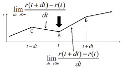
Figure 1: The schematic figure for a stochastic trajectory and velocities. There are at least two different possibilities for the velocity at the point A.

In this section, we derive the generalized uncertainty relation for stochastic systems described in SVM. The definitions introduced below are applicable to both of the particle system and the continuum medium.

For the sake of the unified description, we introduce the notation for the average with respect to the stochastic events and the mass distribution as

$$\left\{A\right\}_{av}=\left\{\begin{array}[c]{ccl}E[A]&&\mathrm{for\ the\ particle\ system}\\ \int d^{3}\mathbf{R}\ \frac{\rho^{0}_{m}(\mathbf{R})}{m}E[A]&&\mathrm{for\ the\ continuum\ medium}.\end{array}\right.$$ (47)

With this, it is natural to define the standard deviation of the position by

$$\Delta_{x^{i}}=\frac{1}{N}\sqrt{\left\{(r^{i}-\left\{r^{i}\right\}_{av})^{2}\right\}_{av}},$$ (48)

with the normalization factor,

$$N=\left\{\begin{array}[c]{ccl}1&&\mathrm{for\ the\ particle\ system}\\ \int d^{3}\mathbf{R}\ \frac{\rho^{0}_{m}(\mathbf{R})}{m}&&\mathrm{for\ the\ continuum\ medium}.\end{array}\right.$$ (51)

Thus, this represents the standard deviation of the position for the particle and that of the center of mass for the continuum medium, respectively.

On the other hand, because of the two different quantities $\mathbf{p}$ and $\bar{\mathbf{p}}$, the definition of the standard deviation for the momentum is not straightforward in SVM. The appearance of the two momenta is associated with the two possible definitions of the velocities which come from the lack of the differentiability of the stochastic trajectories as is shown in Fig. 1: there are two different inclinations of the particle trajectory at the point A, ${\displaystyle\lim_{dt\rightarrow 0_{+}}({r}(t+dt)-{r}(t))/dt}$ and ${\displaystyle\lim_{dt\rightarrow 0_{+}}({r}(t-dt)-{r}(t))/(-dt)}$. These two limits generally do not coincide in stochastic systems. See also the discussion for the uncertainty principle in the original paper by Heisenberg heisenberg .

As is seen from the stochastic Newton equations (27) and (42), the two momenta contribute the evolutions of the particle and of the fluid element on an equal footing, independently of the choice of the parameters $\alpha_{1}$ and $\alpha_{2}$. Therefore, it will be adequate to define the standard deviation of the momentum by the symmetric average of the two standard deviations for $\mathbf{p}$ and $\bar{\mathbf{p}}$ as

$$\Delta_{p^{i}}\equiv\sqrt{\frac{\left\{(p^{i}-\left\{p^{i}\right\}_{av})^{2}\right\}_{av}+\left\{(\bar{p}^{i}-\left\{\bar{p}^{i}\right\}_{av})^{2}\right\}_{av}}{2}}.$$ (52)

The above definitions reproduce the standard deviation in quantum mechanics, as is shown in Appendix A.

To calculate the standard deviation of the momentum, we introduce the sum and the subtraction of the two momenta,

$$\mathbf{p}_{+}\equiv\frac{\mathbf{p}+\bar{\mathbf{p}}}{2}\ \ \ \ \ \mathbf{p}_{-}\equiv\frac{\mathbf{p}-\bar{\mathbf{p}}}{2},$$ (53)

respectively. Moreover, using the Cauchy-Schwarz inequality, we can show that $\{{A}^{2}\}_{av}\{{B}^{2}\}_{av}\geq|\{{AB}\}_{av}|^{2}$ for real stochastic variables ${A}$ and ${B}$. Then we find the following inequalities,

$$\Delta_{x^{i}}\Delta_{p_{+}^{j}}\geq\frac{m}{N}\left|\left\{(r^{i}-\left\{r^{i}\right\}_{av})(u_{m}^{j}-\left\{u_{m}^{j}\right\})\right\}_{av}-\mu N\delta_{ij}\right|,$$ (54)

$$\Delta_{x^{i}}\Delta_{p_{-}^{j}}\geq\frac{m}{\nu N}\left|\mu\left\{(r^{i}-\left\{r^{i}\right\}_{av})(u_{m}^{j}-\left\{u_{m}^{j}\right\}_{av})\right\}_{av}-\kappa N\delta_{ij}\right|,$$ (55)

where $\Delta_{{p}_{\pm}^{j}}=\sqrt{\left\{({p}_{\pm}^{j}-\left\{{p}_{\pm}^{j}\right\}_{av})^{2}\right\}_{av}}$. The standard deviation of the momentum defined above can be expressed as $\Delta_{p^{i}}=\sqrt{\Delta_{p^{i}_{+}}^{2}+\Delta_{p^{i}_{-}}^{2}}$. Therefore, the product of the standard deviations of the position and the momentum satisfies the following inequality,

$$\Delta_{x^{i}}\Delta_{p^{j}}$$

$$\geq\frac{m}{N}\sqrt{\left(1+\left(\frac{\mu}{\nu}\right)^{2}\right)(A^{ij})^{2}+N^{2}\frac{(\kappa-\mu^{2})^{2}}{\nu^{2}+\mu^{2}}\delta_{ij}}$$ (56)

$$\geq m\nu\chi\delta_{ij},$$ (57)

where

$$A^{ij} = \left\{(r^{i}-\left\{r^{i}\right\}_{av})(u_{m}^{j}-\left\{u_{m}^{j}\right\}_{av})\right\}_{av}$$ (58)

$$-\delta_{ij}\frac{\mu N(\kappa+\nu^{2})}{\nu^{2}+\mu^{2}},$$

$$\chi = \frac{4}{\sqrt{1+(\mu/\nu)^{2}}}|\mathrm{det}~{}(M)|,$$ (59)

and $\mathrm{det}~{}(M)$ is calculated from Eq. (18) as

$$\mathrm{det}~{}(M)=\frac{\kappa-\mu^{2}}{4\nu^{2}}.$$ (60)

This inequality is our main result and represents the generalized uncertainty relation satisfied for quantum and stochastic systems formulated in SVM.

As was mentioned, we need to set $(\alpha_{1},\alpha_{2},\nu)=(0,\ 1/2,\ \hbar/(2m))$ to reproduce the Schrödinger equation. Then the above standard deviation of the momentum agree with the well-known expression in quantum mechanics, $\Delta_{p^{i}}=\sqrt{\langle(\hat{p}^{i}-\langle\hat{p}^{i}\rangle)^{2}\rangle}$ where $\hat{p}^{i}=-i\hbar\partial_{x^{i}}$ and $\langle\ \ \rangle$ denotes the expectation value with a wave function. See Appendix A for details. Therefore Eq. (57) reproduces the uncertainty relation in quantum mechanics called Kennard inequality, $\Delta_{x^{i}}\Delta_{p^{j}}\geq\frac{\hbar}{2}\delta_{ij}$.

One should remember that the optimization in SVM reproduces the result of the classical variation in vanishing limit of $\nu$. Therefore one can easily see the trivial result that the finite minimum uncertainty disappears in classical systems. On the contrary, the finiteness of the minimum uncertainty is held for any stochastic dynamics with a finite $\nu$ because $\mathrm{det}~{}(M)\neq 0$ for any $(\alpha_{1},\alpha_{2})$.

III.1 Robertson-Schrödinger uncertainty relation

As a more general uncertainty relation, there exists the Robertson-Schrödinger uncertainty relation. When this uncertainty relation is applied to the position and momentum operators, we find the following inequality,

$$\Delta^{2}_{x^{i}}\Delta^{2}_{p^{j}} \geq \frac{\hbar^{2}}{4}+\left|\frac{1}{2}\langle[\hat{x}^{i},\hat{p}^{j}]_{+}\rangle-\langle\hat{x}^{i}\rangle\langle\hat{p}^{j}\rangle\right|^{2}$$ (61)

$$= \frac{\hbar^{2}}{4}+({\rm Re}[\langle(\hat{x}^{i}-\langle\hat{x}^{i}\rangle)(\hat{p}^{j}-\langle\hat{p}^{j}\rangle)])^{2},$$

where $[~{}]_{+}$ denotes the anti-commutator.

On the other hand, when we employ the parameters to reproduce the quantum mechanical results in SVM. the same result can be obtained from Eq. (56), noting that

$$\left\{(r^{i}-\left\{r^{i}\right\}_{av})(u_{m}^{j}-\left\{u_{m}^{j}\right\}_{av})\right\}_{av}$$ (62)

$$= \frac{1}{m}{\rm Re}[\langle(\hat{x}^{i}-\langle\hat{x}^{i}\rangle)(\hat{p}^{j}-\langle\hat{p}^{j}\rangle)].$$

Therefore the Robertson-Schrödinger uncertainty relation is obtained when Eq. (56) is used while the Kennerd inequality is derived for Eq. (57).

IV Application to continuum media

So far, two examples in the continuum media are known to be described in the framework of SVM: one is the Gross-Pitaevskii equation and the other the Navier-Stokes-Fourier equation. We study our uncertainty relations in these cases.

IV.1 Gross-Pitaevskii equation

In the usual derivation of the Gross-Pitaevskii equation, we start from the bosonic system described by the following Hamiltonian operator,

$$\hat{H} = \int d^{3}\mathbf{x}\left[\frac{\hbar^{2}}{2m}\nabla\hat{\phi}^{\dagger}(\mathbf{x})\cdot\nabla\hat{\phi}(\mathbf{x})+V(\mathbf{x})\hat{\phi}^{\dagger}(\mathbf{x})\hat{\phi}(\mathbf{x})\right.$$ (63)

$$\left.+\frac{U_{0}}{2}(\hat{\phi}^{\dagger}(\mathbf{x})\hat{\phi}(\mathbf{x}))^{2}\right],$$

where $m$, $V(\mathbf{x})$ and $U_{0}$ are the mass of an atom, an external potential and the coupling constant of the two-body interaction, respectively. The bosonic field operator satisfies

$$[\hat{\phi}(\mathbf{x},t),\hat{\phi}^{\dagger}(\mathbf{x}^{\prime},t)]=\delta^{(3)}(\mathbf{x}-\mathbf{x}^{\prime}).$$ (64)

By applying the mean-field approximation to this quantum-field theoretical system, we obtain the Gross-Pitaevskii equation which describes the behavior of the Bose-Einstein condensate of the ultracold atom.

The same equation can be obtained in a different way. Let us consider a classical gas composed of $N$ particles. To describe the exact behavior of the gas, we need to solve the $N$-body Newton equations. On the other hand, when we are interested in only macroscopic behaviors of the gas, we do not need to know the positions and velocities of the particles. Instead, it is sufficient to observe the behaviors of the reduced number of macroscopic variables: the mass density and the velocity field. Then the many-body particle system is regarded as a continuum medium. The approximated quantum dynamics of such a many-body system can be obtained by applying SVM to the Lagrangian of the continuum medium kk2 .

Let us consider the situation in the ultracold atom, choosing the internal energy density in Eq. (34) as

$$\varepsilon(\rho_{m}(\mathbf{x},t))=\frac{U_{0}}{2}\frac{\rho^{2}_{m}(\mathbf{x},t)}{m^{2}}.$$ (65)

Other parameters are the same as those in the case of the Schrödinger equation; $(\alpha_{1},\alpha_{2},\nu)=(0,\ 1/2,\ \hbar/(2m))$. Substituting these into Eqs. (5) and (43) and defining the wave function $\psi(\mathbf{x},t)$ in the same way as Eq. (32), the Gross-Pitaevskii equation is reproduced,

$$i\hbar\partial_{t}\psi(\mathbf{x},t)=\left[-\frac{\hbar^{2}}{2m}\nabla^{2}+V(\mathbf{x})+U_{0}|\psi(\mathbf{x},t)|^{2}\right]\psi(\mathbf{x},t),$$ (66)

See Ref. kk2 for more details.

Now, by using Eq. (57), the uncertainty relation obtained from our formula is expressed as

$$\Delta_{x^{i}}\Delta_{p^{j}}\geq\frac{\hbar}{2}\delta_{ij}.$$ (67)

This inequality is the same as the one obtained in the quantum field theory from Eq. (64), where the standard deviations are represented by

$$\Delta_{x^{i}} =\frac{1}{\langle\int d^{3}\mathbf{x}\ \hat{\phi}^{\dagger}(\mathbf{x},t)\hat{\phi}(\mathbf{x},t)\rangle}\sqrt{\langle(\hat{x}^{i})^{2}\rangle-\langle\hat{x}^{i}\rangle^{2}},$$ (68)

$$\Delta_{p^{i}} =\sqrt{\langle(\hat{p}^{i})^{2}\rangle-\langle\hat{p}^{i}\rangle^{2}},$$ (69)

$$\hat{\mathbf{x}} =\int d^{3}\mathbf{x}\hat{\phi}^{\dagger}\mathbf{x}\hat{\phi},$$ (70)

$$\hat{\mathbf{p}} =\int d^{3}\mathbf{x}\hat{\phi}^{\dagger}(-i\hbar\nabla)\hat{\phi},$$ (71)

where $\langle\ \ \rangle$ denotes the expectation value with a state vector in a Fock space. That is, our uncertainty relation is consistent with that of the quantum field theory.

As a different derivation of the Gross-Pitaevskii equation in SVM, see Ref. loffred . The bosonic field quantization in the framework of SVM is studied in Ref. svm-field .

IV.2 Navier-Stokes-Fourier equation

So far we have exclusively considered the case where the noise term is interpreted as the origin of the quantum fluctuations where $\nu=\hbar/(2m)$. Now we consider a classical stochastic system where $\nu$ characterizes the intensity of the thermal fluctuations and thus is given by a function of temperature. We further choose the parameters $\alpha_{2}=0$, then $\kappa$ vanishes and our optimized equation (43) is reduced to

$$\rho_{m}\left(\partial_{t}+\mathbf{u}_{m}\cdot\nabla\right)\mathbf{u}_{m}-\nabla\cdot(\eta\widehat{E})=-\nabla P.$$ (72)

Here we take $V=0$ for the sake of simplicity. Then $\eta\widehat{E}$ represents the stress tensor and this is the Navier-Stokes-Fourier equation . We introduced the coefficient of viscosity $\eta=\mu\rho_{m}$. Then $\mu=\alpha_{1}\nu=\eta/\rho_{m}$ is known as kinematic viscosity.

In the modern perspective in statistical mechanics, the macroscopic dissipation (viscosity) is induced by the fluctuation of the underlying microscopic degrees of freedom. This property results in the fluctuation-dissipation theorem. We can consider that the SVM formulation of the Navier-Stokes-Fourier equation naturally reflects this aspect. Moreover the coefficient of viscosity is formally expressed with the velocity (current) correlation function of the constituent particles,

$$\mu=\frac{\alpha_{1}}{3N}\int_{-\infty}^{\infty}dt\theta(t)\left\{\delta\mathbf{v}(\mathbf{r},t)\cdot\delta\mathbf{v}(\mathbf{r},0)\right\}_{av},$$ (73)

with $\delta\mathbf{v}(\mathbf{r},t)=d\mathbf{r}(\mathbf{R},t)/dt-\mathbf{u}(\mathbf{r}(\mathbf{R},t))$.

Substituting these parameters into our inequality (57), the uncertainty relation for hydrodynamics is given by

$$\Delta_{x^{i}}\Delta_{p^{j}}\geq\frac{m\mu^{2}}{\sqrt{\mu^{2}+\nu^{2}}}\delta_{ij}.$$ (74)

Note that the standard deviations can be expressed as the averages with respect to the mass density distribution because, for an arbitrary function $F(\mathbf{x},t)$, $\left\{F(\mathbf{r}(\mathbf{R},t),t)\right\}_{av}=\int d^{3}\mathbf{x}\ \frac{\rho_{m}(\mathbf{x},t)}{m}F(\mathbf{x},t)$.

Equation (74) means that the minimum uncertainty becomes larger as the increase of the viscosity of the fluid. This is reasonable, because due to the fluctuation-dissipation theorem, larger fluctuation induces higher viscosity and vice-versa.

The dimension of $\mu$ and $\nu$ is $L^{2}T^{-1}$ and, for a macroscopic fluid, the magnitude of $\mu$ which represents the viscosity of fluids, is of the order of the macroscopic scale. On the other hand, $\nu$ is the noise intensity in the microscopic dynamics described by Eq. (1). Then the magnitude of the associated distance ($L$) is the microscopic scale, while that of $LT^{-1}$ should be, at a maximum, of the order of the sound velocity. Thus the magnitude of $\nu$ is expected to be much smaller than that of $\mu$. Let us estimate the minimum uncertainty, for example, of water. Assuming the simple fluid, $m$ is equivalent to the mass of the water molecule, $\sim 3\times 10^{-26}$ kg. The kinematic viscosity at room temperature is $\sim 1\times 10^{-6}$ $m^{2}/s$. Then the minimum uncertainty is estimated as

$$\frac{m\mu^{2}}{\sqrt{\mu^{2}+\nu^{2}}}\sim m\mu\sim 3\times 10^{-32}\ [kg\ m^{2}/s^{2}]\sim 100\times\frac{\hbar}{2}.$$ (75)

This value is two orders larger than that of quantum mechanics but is still much smaller than the (coarse-grained) macroscopic scales of hydrodynamics. To observe this uncertainty for a fluid, we need to measure the mass distribution and the velocity field of fluids with precision. In such a precision, however, the hydrodynamic description normally looses its validity because the hydrodynamic approach is applicable only to macroscopic variables observed in a coarse-grained scale which will be much larger than $\hbar$. See also the discussion in Sec. V.

IV.2.1 The possible role of the $\kappa$ term in hydrodynamics

In the discussion above, we set $\alpha_{2}=0$ to ignore the coefficient $\kappa=2\alpha_{2}\nu$ because such a term is usually considered to be irrelevant to the dynamics of fluids, while the same term, which is called quantum potential, plays an important role in the hydrodynamic representation of the Schödinger equation holland (See the last term on the left hand side of Eq. (29)). Recently, Brenner pointed out that, since the velocity of a tracer particle of fluids is not necessarily parallel to the mass velocity, the existence of these two velocities should be taken into account in the formulation of hydrodynamics. By applying the linear irreversible thermodynamics, then, it is found that the difference of the two velocities are characterized by the mass density gradient as is our self-consistency condition (7) and a new term analogous to the quantum potential can appear. This modified theory is called the bivelocity hydrodynamics brenner1 ; brenner2 . The similar results are obtained in various approaches including SVM, but the existence is still controversial klimontovich ; ottinger ; graur ; greensh ; eu ; don ; dadzie ; kk2 ; gustavo . See also TABLE 1 of Ref. brenner2 . It is also worth mentioning that the structure which is the same as the bivelocity hydrodynamics naturally appears as the next-to-leading order relativistic corrections to the Navier-Stokes-Fourier equation gustavo .

Another possible role of the $\kappa$ term is related to the sign of the kinetic term in the stochastic Lagrangian. To obtain the Navier-Stokes-Fourier equation, we chose $\alpha_{1}>0$ and $\alpha_{2}=0$, leading to

$$\mathrm{Tr}~{}(M)>0~{}\mathrm{and}~{}\det~{}(M)<0,$$ (76)

where $M$ is the two-by-two matrix (18) appearing in the stochastic Lagrangian. On the other hand, from the well-known second-order algebra, the necessary and sufficient condition for the positive-semidefinite kinetic term in Eq. (21) (or equivalently Eq. (38)) is given by

$$\mathrm{Tr}~{}(M)>0~{}\mathrm{and}~{}\det~{}(M)>0,$$ (77)

and it demands

$$\mu<\sqrt{\kappa}.$$ (78)

Therefore, to have a finite viscosity requiring the positive kinetic term, $\kappa$ should be finite. Note, however, that it is not clear whether such a requirement is mandatory, because the above positivity is irrelevant to the positivity of the fluid energy, $\int d^{3}\mathbf{x}\left[\frac{1}{2}\rho_{m}(\mathbf{x},t)\mathbf{u}^{2}_{m}(\mathbf{x},t)+\varepsilon(\rho_{m}(\mathbf{x},t))\right]$ which is positive independently of the value of $\kappa$.

This $\kappa$ term may play an important role in applying the hydrodynamic model to microscopic systems such as relativistic heavy-ion collisions, as is discussed in Sec. V.

V Concluding remarks

We discussed the uncertainty relation satisfied for general stochastic systems which are described in the stochastic variational method. We first developed the Hamiltonian formulation of SVM. Then we introduced the two different momenta through the Legendre transformation of the stochastic Lagrangian. Because the contributions from the two momenta are the same in the stochastic Newton equation, the standard deviation of the momentum should be defined by the symmetric average of the standard deviations of those momenta. Using this, we derived the generalized uncertainty relation satisfied for stochastic systems described in SVM. When we choose the parameter set which reproduces the Schödinger equation, our uncertainty relation is reduced to the Kennard inequality in quantum mechanics. Note that the SVM quantization does not always reproduce the same result as the canonical quantization. As an example, see Appendix B.

The stochastic generalization of the variational principle indicates that we need to use the two optimizations quite differently, depending on the hierarchy of observation scales in physics. Suppose that we obtain an equation by optimizing an action. When we observe a system with a macroscopic scale where we can ignore the possible zig-zag motion, it is sufficient to use classical variation for the optimization. However, when we are interested in more precise behaviors in a microscopic scale and hence we cannot ignore the non-differentiable trajectories in the optimization of the same action, the stochastic variation should be employed.

In this paper, we have focused on the uncertainty relation of the position and the momentum. To obtain the uncertainty relation of, for example, the angle and the angular momentum, we have to express Eq. (1) in the spherical coordinate but then the transformation law of the standard Wiener process ${\bf W}_{t}$ is non-trivial. See, for example, Ref. gardinar . The generalization of the present formulation for such a case is left as a future work.

Applying the present approach to the continuum media, we investigated the uncertainty relation for the Gross-Pitaevskii equation and the Navier-Stokes-Fourier equation. For the former, we confirmed that our result is the same as that obtained in the quantum field theory. For the latter, we found that the minimum uncertainty is enhanced as the increase of the viscosity. This is a reasonable behavior because, from the fluctuation-dissipation theorem, higher viscosity indicates larger fluctuation and vice-versa. For the water at room temperature, the minimum uncertainty becomes two orders of magnitude larger than that of quantum mechanics, $\hbar/2$. It is however much smaller than the (coarse-grained) macroscopic scales of hydrodynamics and thus the effect of the minimum uncertainty is negligible in the usual fluids. In our formulation, the minimum uncertainty never disappear for any stochastic systems, independently of the values of $(\mu,\kappa)$ when the momenta are well-defined. Therefore, we can consider that the finite minimum uncertainty between the position and the momentum is not an inherent feature in quantum mechanics but a common feature in stochastic systems described in SVM.

However, the existence of the minimum uncertainty for continuum media shows that a special care should be taken when a hydrodynamic approach is applied to microscopic systems. For example, the hydrodynamic models are often employed to describe the behaviors of the hot matters created in relativistic heavy-ion collisions review-kodama . Although the uncertainty relation for the relativistic fluid is not obtained here, it is reasonable to assume that the minimum value cannot be smaller than the quantum mechanical one, $\hbar/2$. The global size of the initially produced fluid is the order of 10 fm, but the distribution of the energy density is expected to be inhomogeneous and presents many local peaks review-kodama . To describe such a peak as a fluid, the uncertainty of the position of the fluid elements must be smaller than the size of the peaks, say, $10^{-1}$ fm. Therefore the expected uncertainty of the momentum becomes, at least, $\sim 1$ GeV/c. If we attribute this fluctuation to the pure thermal origin without any quantum effect, then the corresponding temperature would be much larger than $\sim 1$ GeV/$k_{B}$ $\sim 10^{13}$ K. Such a temperature far exceeds what we usually expect in the relativistic heavy-ion collisions. However, as is seen from the form of the $\kappa$ term (quantum potential), the effect of the quantum fluctuation is extremely enhanced near the large inhomogeneities. Therefore, if we employ a relativistic hydrodynamic approach to describe the above situation, it will be necessary to consider a model which incorporates dynamically the enhanced quantum effect near the inhomogeneity. Then in the presence of a sharp peak, the generated pressure should be attributed not only to a high temperature of the hot matter, but also to the quantum fluctuation. Such effects are expected to be important to shed a new light to understand the collective dynamics observed in small systems as proton-nucleon and proton-proton collisions.

Appendix A Relation to quantum mechanical standard deviation

We will show that Eq. (52) is equivalent to that in quantum mechanics. See also the discussion in Ref. falco . First we find the second order correlation of the momentum operator in quantum mechanics as

$$\langle\hat{\mathbf{p}}^{2}\rangle = \langle\hbar^{2}(\nabla R(\mathbf{x},t))^{2}+(\nabla S(\mathbf{x},t))^{2}\rangle,$$ (79)

where $\langle~{}~{}~{}\rangle$ represents the expectation value with the wave function $\psi(\mathbf{x},t)=e^{R(\mathbf{x},t)-iS(\mathbf{x},t)/\hbar}$ with the real functions $R(\mathbf{x},t)$ and $S(\mathbf{x},t)$. On the other hand, Eq. (7) is re-expressed with this decomposition of the wave function as $\mathbf{u}(\mathbf{x},t)-\tilde{\mathbf{u}}(\mathbf{x},t)=2\hbar\nabla R(\mathbf{x},t)/m$. Note that the current of the probability density is equivalent to that of the Fokker-Planck equation. Therefore the mean velocity is expressed as $\mathbf{u}_{m}(\mathbf{x},t)=\nabla S/m(\mathbf{x},t)$.

Using these relations, we can show that $E[(m\mathbf{u})^{2}+(m\tilde{\mathbf{u}})^{2}]/2=\langle\hat{\mathbf{p}}^{2}\rangle$ and $E[m\mathbf{u}]=E[m\tilde{\mathbf{u}}]=\langle\nabla S\rangle/m=\langle\hat{\mathbf{p}}\rangle$. Summarizing these results, we find

$$(\Delta_{\mathbf{p}})^{2}=\langle\hat{\mathbf{p}}^{2}\rangle-\langle\hat{\mathbf{p}}\rangle^{2}$$

$$=\frac{E[(m\mathbf{u})^{2}]-(E[m\mathbf{u}])^{2}}{2}+\frac{E[(m\tilde{\mathbf{u}})^{2}]-(E[m\tilde{\mathbf{u}}])^{2}}{2}.$$ (80)

For the case of quantum mechanics where $(\alpha_{1},\alpha_{2})=(0,1/2)$ and $\nu=\hbar/(2m)$, we have $\mathbf{p}=m\mathbf{u}$ and $\bar{\mathbf{p}}=m\tilde{\mathbf{u}}$. Therefore the right hand side of the above result is equivalent to Eq. (52).

Appendix B Uncertainty relation for quantum dissipative system

There is an example where SVM leads to the different result from the canonical quantization misawa ; skag . We consider the following time-dependent Lagrangian,

$$L({r},\dot{r},t)=e^{\gamma t}\left[\frac{m}{2}\left(\frac{d{r}(t)}{dt}\right)^{2}-V({r}(t))\right],$$ (81)

where $\gamma$ is a constant which characterizes the time scale of the relaxation of a particle with the mass $m$. It is easily confirmed that we obtain a dissipative equation from this Lagrangian by applying the classical variational method.

The canonical quantization of this system was studied by Caldirola caldi and Kanai kanai , leading to the following Schrödinger equation,

$$i\hbar\psi=\left[-\frac{\hbar^{2}}{2m}e^{-\gamma t}\partial^{2}_{x}+e^{\gamma t}V({x})\right]\psi,$$ (82)

defining the momentum operator $\hat{p}=-i\hbar\partial_{x}$. Therefore, the corresponding uncertainty relation is

$$\Delta_{x}\Delta_{p}\geq\frac{\hbar}{2}.$$ (83)

The SVM quantization of the same Lagrangian was studied in Ref. misawa . The stochastic Lagrangian is then expressed as

$$L({r},D{r},\tilde{D}{r},t)=e^{\gamma t}\left[m\frac{(D{r}(t))^{2}+(\tilde{D}{r}(t))^{2}}{4}-V({r}(t))\right].$$ (84)

We consider that ${r}(t)$ satisfies the same stochastic differential equations (1) and (6), and $\nu=\hbar/(2m)$. Then the stochastic variation leads to

$$i\hbar\partial_{t}\psi=\left[-\frac{\hbar^{2}}{2m}\partial^{2}_{x}+V({x})+\frac{i\hbar}{2}\gamma\ln\frac{\psi^{*}}{\psi}+a(t)\right]\psi,$$ (85)

where $a(t)$ is an arbitrary time-dependent factor, which can be absorbed into the definition of the phase misawa . This non-linear Schrödinger equation coincides with the so-called Kostin (or Schrödinger-Langevin) equation kostin ; dekker ; hasse by choosing $a(t)=-\frac{i\hbar}{2}\gamma\left\langle\ln(\psi^{*}/\psi)\right\rangle$ where $\langle~{}~{}\rangle$ means the expectation value with $\psi$.

In the original approach by Kostin, this equation is derived phenomenologically to satisfy Eherenfest’s theorem and hence the definition of the momentum operator is not clear. On the other hand, applying the method developed in this paper, we find

$$\Delta_{x}\Delta_{p}\geq\frac{\hbar}{2}e^{\gamma t},$$ (86)

where the momentum operator is obtained by the stochastic Noether theorem kkk , finding $\hat{p}=-i\hbar e^{\gamma t}\partial_{x}$.

As is seen from the right hand side, the minimum uncertainty increases with time. This behavior is different from the Caldirola-Kanai theory, but in reality, the behavior of Eq. (83) is considered to be problematic. Following the discussion in Refs. dekker ; hasse ; brittin ; havas ; sent , the uncertainty of the inertia is defined by $\Delta_{inertia}=e^{-\gamma t}\Delta_{p}$ and then Eq. (83) leads to the following minimum uncertainty of the inertia,

$$\Delta_{x}\Delta_{inertia}\geq\frac{\hbar}{2}e^{-\gamma t}.$$ (87)

It shows that the uncertainty vanishes in the asymptotic limit in time and this behavior is sometimes considered to be unphysical dekker ; hasse ; brittin ; havas ; sent . On the other hand, such a behavior does not occur in our result (86).

It should be, however, noted that the above violation of the uncertainty relation is still controversial. In Ref. dieter , it is argued that if we change the definition of the momentum operators by multiplying or dividing a factor $e^{\gamma t}$ as was done to define the uncertainty of the inertia, we need to change also the Hilbert space. If this possibility is taken into account, the minimum uncertainty for the inertia in the Caldirola-Kanai theory does not vanish asymptotically.

There is no established method for the systematic quantization of dissipative systems and the aforementioned theories are only one part of various approaches. As other approaches, see, for example, Refs. dieter2 ; goldin ; marcelo ; blasone and references therein.

References

- (1) K. Yasue, J. Funct. Anal. 41 (1981) 327.
- (2) As the non-differentiable trajectory in the path integral formulation, see B. Koch and I. Reyes, Int. J. Geom. Methods Mod. Phys. 12 (2015) 1550100.
- (3) F. Guerra and L. M. Morato, Phys. Rev. D27 (1983) 1774.
- (4) R. Marra, Phys. Rev. D36 (1987) 1724.
- (5) M. Serva, Ann. Inst. Henri Poincaré 49 (1988) 415.
- (6) M. T. Jaekel, J. Phys. A23 (1990) 3497.
- (7) M. Pavon, J. Math. Phys. 36 (1995) 6774.
- (8) H. H. Rosenbrock, Proc. R. Soc. Lond. A450 (1995) 417 ; Proc. R. Soc. Lond. A 453 (1997) 983.
- (9) M. Nagasawa, Stochastic Process in Quantum Physics (Birkhäuser, 2000).
- (10) H. J. Kappen, Phys. Rev. Lett. 95 (2005) 200201.
- (11) D. A. Gomes, Commun. Math. Phys. 257 (2005) 227.
- (12) J. Cresson and S. Darses, J. Math. Phys. 48 (2007) 072703.
- (13) G. L. Eyink, Physica D 239 (2010) 1236.
- (14) M. Arnaudon and A. B. Cruzeiro, Bull. Sci. Math. 136 (2012) 857.
- (15) X. Chen, A. B. Cruzeiro, and T. S. Ratiu, arXiv:1506.05024.
- (16) D. D. Holm, Proc. R. Soc. Lond. A 471 (2015) 20140963.
- (17) J. C. Zambrini, Int. J. Theor. Phys. 24 (1985) 277.
- (18) T. Koide, T. Kodama and K. Tsushima, J. Phys.: Conf. Ser. 626 (2015) 012055.
- (19) T. Koide, J. Phys.: Conf. Ser. 410 (2013) 012025.
- (20) E. Nelson, Phys. Rev. 150 (1966) 1079.
- (21) T. Koide and T. Kodama, J. Phys. A: Math. Theor. 45 (2012) 255204.
- (22) T. Koide, Phys. Lett. A 379 (2015) 2007.
- (23) E. Schrödinger, Sitzungsber. Preuss. Akad. Phys. Math. Klasse 1 (1931) 144 .
- (24) E. Schrödinger, Ann. Inst. Henri Poincaré 11 (1932) 300.
- (25) S. Bernstein. Verhand. Internat. Math. Kongr. Zürich (Band I) (1932).
- (26) B. Jamison, Z. Wahrsch. verw. Geb. 30 (1974) 65.
- (27) J. C. Zambrini, Phys. Rev. A 35 (1987) 3631.
- (28) J. C. Zambrini, Phys. Lett. B 151 (1988) 327.
- (29) S. Albeverio, K. Yasue and J. C. Zambrini, Ann. Inst. Henri Poincaré A50 (1989) 259.
- (30) P. Garbaczewski and J.-P. Vigier, Phys. Lett. A167 (1992) 445.
- (31) C. Léonaed, S. Rcelly and J.-C. Zambrini, arXiv:1308.0576.
- (32) C. Léonard, Discrete and Continuous Dynamical Systems - Series A 34 (2013) 1533.
- (33) T. Koide, J. Phys. Commun. 2 (2018) 021001.
- (34) T. Misawa, J. Math. Phys. 29 (1988) 2178.
- (35) E. Nelson, Lect. Notes in Physics 262 (1986) 109.
- (36) T. Misawa and K. Yasue, J. Math. Phys. 28 (1987) 2569.
- (37) A. Caticha, J. Phys. A: Math. Theor. 44 (2011) 225303.
- (38) M. Davidson, Lett. Math. Phys. 3 (1979) 271.
- (39) H. Hasegawa, Phys. Rev. D 33 (1986) 2508.
- (40) J. H. Gaspar Elsas, T. Koide and T. Kodama, Braz. J. Phys. 45 (2015) 334.
- (41) H.-T. Elze, et al. J. Phys. G25 (1999) 1935.
- (42) W. Heisenberg, Z. Phys. 43 (1927) 172.
- (43) M. I. Loffredo and L. M. Morato, J. Phys. A: Math. Theor. 40 (2007) 8709.
- (44) T. Koide and T. Kodama, Prog. Theor. Exp. Phys. 2015, 093A03.
- (45) See, for example, P. R. Holland, The Quantum Theory of Motion: An Account of the de Broglie-Bohm Causal Interpretation of Quantum Mechanics (Cambridge University Press, Cambridge, UK, 1995).
- (46) H. Brenner, Phys. Rev. E70 (2004) 061201.
- (47) H. Brenner, Phys. Rev. E86 (2012) 016307 and references therein.
- (48) Y. L. Klimontovich, Theor. Math. Phys. 92 (1992) 909.
- (49) H. C. Ottinger, Beyond Equilibrium Thermodynamics (Wiley, Hoboken, NJ, 2005).
- (50) I. A. Graur, J. G. Méolens and D. E. Zeitoun, Microfluid Nanofluid 2 (2006) 64.
- (51) C. J. Greenshields and J. M. Reese, J. Fluid Mech. 580 (2007) 407.
- (52) B. C. Eu, J. Chem. Phys. 129 (2008) 094502.
- (53) N. Dongari, F. Durst, S. Chakraborty, Microfluid. Nanofluid. 9 (2010) 831.
- (54) S. K. Dadzie, J. M. Reese and C. R. McInnes, Physica A 387 (2008) 6079.
- (55) T. Koide, R. O. Ramos and G. S. Vicente, Braz. J. Phys. 45 (2015) 102.
- (56) C. W. Gardiner, Handbook of Stochastic Method (Springer,2004).
- (57) R. Derradi de Souza, T. Koide and T. Kodama, Prog. Part. Nucl. Phys. 86 (2016) 35.
- (58) D. de Falco, S. De Martino and S. De Siena, Phys. Rev. Lett. 49 (1982) 181.
- (59) T. Misawa, Phys. Rev. A 40 (1989) 3387.
- (60) Bo-Sture K. Skagerstam, J. Math. Phys. 18 (1977) 308.
- (61) P. Caldirola, Nuovo Cimento 18 (1941) 393.
- (62) E. Kanai, Prog. Theor. Phys. 3 (1948) 440.
- (63) M. D. Kostin, J. Chem. Phys. 57 (1972) 3589.
- (64) H. Dekker, Phys. Rep. 80 (1981) 1.
- (65) R. W. Hasse, J. Math. Phys. 16 (1975) 2005.
- (66) W. E. Brittin, Phys. Rev. 77 (1950) 396.
- (67) I. R. Senitzky Phys. Rev. 119 (1960) 670.
- (68) P. Havas, Bull. Am. Phys. Soc. 1 (1956) 337.
- (69) D. Schuch, Phys. Rev. A 55 (1997) 935.
- (70) D. Schuch, K.-M. Chung, Int. J. Quantum Chem. 29 (1986) 1561.
- (71) H.-D. Doebner and G. A. Goldin, Phys. Lett. A162 (1992) 397.
- (72) M. A. Marchiolli and S. S. MIzrahi, J. Phys. A:Math. Gen. 30 (1997) 2619.
- (73) M. Blasone, O. Jizba and G. Vitiello, Phys. Lett. A287 (2001) 205.
- (74) T. Takabayasi, Prog. Theor. Phys. 9 (1953) 187.
- (75) T. C. Wallstrom, Found. Phys. Lett. 2 (1989) 113.
- (76) M. Derakhshani, arXiv:1510.06391.