Dynamical evolution of the Gliese 436 planetary system

Abstract

Context. The close-in planet orbiting GJ 436 presents a puzzling orbital eccentricity ($e\simeq 0.14$) considering its very short orbital period. Given the age of the system, this planet should have been tidally circularized a long time ago. Many attempts to explain this were proposed in recent years, either involving abnormally weak tides, or the perturbing action of a distant companion.

Aims. In this paper, we address the latter issue based on Kozai migration. We propose that GJ 436b was formerly located further away from the star and that it underwent a migration induced by a massive, inclined perturber via Kozai mechanism. In this context, the perturbations by the companion trigger high amplitude variations to GJ 436b that cause tides to act at periastron. Then the orbit tidally shrinks to reach its present day location.

Methods. We numerically integrate the 3-body system including tides and General Relativity correction. We use a modified symplectic integrator as well a fully averaged integrator. The former is slower but accurate to any order in semi-major axis ratio, while the latter is first truncated to some order (4^th) in semi-major axis ratio before averaging.

Results. We first show that starting from the present-day location of GJ 436b inevitably leads to damping the Kozai oscillations and to rapidly circularizing the planet. Conversely, starting from 5-10 times further away allows the onset of Kozai cycles. The tides act in peak eccentricity phases and reduce the semi-major axis of the planet. The net result is a two fold evolution, characterized by two phases: a first one with Kozai cycles and a slowly shrinking semi-major axis, and a second one once the planet gets out of the Kozai resonance characterized by a more rapid decrease. The timescale of this process appears in most cases much longer than the standard circularization time of the planet by a factor larger than 50.

Conclusions. This model can provide a solution to the eccentricity paradox of GJ 436b. Depending on the various orbital configurations (mass and location o the perturber, mutual inclination…), it can take several Gyrs to GJ 436b to achieve a full orbital decrease and circularization. According to this scenario, we could be witnessing today the second phase of the scenario where the semi-major axis is already reduced while the eccentricity is still significant. We then explore the parameter space and derive in which conditions this model can be realistic given the age of the system. This yields constraints on the characteristics of the putative companion.

1 Introduction

The M-dwarf GJ 436 has been the subject of growing interest in recent years. This star is known to host a close-in Neptune-mass planet (Gl 436b Butler et al. 2004) that was furthermore observed to undergo transit (Gillon et al. 2007).

The monitoring of the transits of GJ 436b helped constraining its orbital solution. Noticeably, it appears to have a significant non-zero eccentricity: $e=0.14\pm 0.1$ (Maness 2007), furthermore refined to $e=0.14\pm 0.01$ (Demory et al. 2007). This eccentricity is abnormally high for a small period planet ($P\simeq 2.64\,$days Ballard et al. 2010). With such a small orbital period, tidal forces are expected to circularize the orbit within much less than the present age of the system (1–10 Gyr Torres 2007). Tidal forces seem indeed to be at work in this system. The detection of the secondary transit of the planet enabled Demory et al. (2007) to derive a brightness temperature of $T=712\pm 36\,$K, with flux reradiated across the day-side only. Conversely, a stellar irradiation / thermal re-radiation balance leads for to an equilibrium temperature for the planet $T_{\mathrm{eq}}=642\,$K, assuming $T_{\mathrm{eff}}=3350$ K for GJ 436 and zero albedo for the planet. According to Deming et al. (2007), the temperature difference indicates tidal heading of GJ 436b, but this could alternatively be due to the $8\,\mu$m sampling the atmosphere in a hot band pass, if the planetary atmosphere does not radiate like a black-body.

Many theories were proposed in recent years to account for the residual eccentricity of GJ 436b. The most straightforward one is that the tides are sufficiently weak and/or the age of the system is small enough to allow a regular tidal circularization not to be achieved yet. This idea was proposed by Mardling (2008) for GJ 436b, after Trilling (2000) had suggested that this accounts for any close-in exoplanet observed with significant eccentricity. It is in fact related to our poor knowledge of the planet’s tidal dissipation $Q_{p}$. $Q_{p}$ is a dimensionless parameter related to the rate of energy dissipated per orbital period by tidal forced oscillations (Barker & Ogilvie 2009). The smaller $Q_{p}$, the more efficient the tidal dissipation is. To lowest order, the circularization time-scale $t_{\mathrm{circ}}$ of an exoplanet reads (Goldreich & Soter 1966; Jackson et al. 2008)

$$t_{\mathrm{circ}}=\frac{4}{63}\frac{a^{13/2}}{\sqrt{GM_{*}^{3}}}{Q_{p}m_{p}}{R_{p}^{5}}\qquad,$$ (1)

where $M_{*}$ is the stellar mass, $a$ is the planet’s orbital semi-major axis, $m_{p}$ its mass and $R_{p}$ its radius. Assuming $Q_{p}=10^{5}$, $R=27,600\,$km, $a=0.0287\,$AU, $m=23.2\,M_{\oplus}$ and $M=0.452\,M_{\odot}$ (Mardling 2008), this formula gives $t_{\mathrm{circ}}=4.7\times 10^{7}\,$yr, which is obviously less than the age of the system. But $Q_{p}$ is very badly constrained. For Neptune, it is estimated between $\sim 10^{4}$ and $3.3\times 10^{5}$ (Banfield & Murray 1992; Zhang & Hamilton 2008). We can thus consider $10^{5}$ as a standard likely value for GJ 436b, but Mardling (2008) argues that $Q_{p}$ could be as high as a few $10^{6}$. In this context, assuming the lower bound (1 Gyr) for the age of the system, the circularization could not be achieved yet. This depends however on the starting eccentricity at time zero. Wisdon (2008) performed analytical calculations of energy dissipation rates for synchronized bodies at arbitrary eccentricities and obliquities. His concluded that for a large enough starting eccentricity ($\ga 0.4$, as will be the case below), the circularization time-scale should be significantly reduced with respect to Eq. (1). In this context, the conclusions by Mardling (2008) may no longer hold. This shows also that conclusions drawn on asymptotic formulas like Eq. (1) must be treated with caution. Numerical work is required.

Alternatively, many authors proposed that the eccentricity of GJ 436b is sustained by perturbations by an outer massive planet, despite a standard $Q_{p}$ value. Such a long period companion was initially suspected as Maness (2007)’s radial velocity data revealed a linear drift. More data did not confirm the trend, which is now believed to be spurious. Montagnier et al. (2012) gives instead observational uppers limits for the putative companion that rule out any companion in the Jupiter mass range up to a few AUs.

Perturbers can be either resonant or non-resonant. Looking for a for a planet locked in mean-motion resonance with GJ 436b appears a promising idea, as resonant configuration usually trigger larger eccentricity modulations. This was suggested by Ribas et al. (2008), who fitted in the residuals of the radial velocity data a $\sim 5\,M_{\oplus}$ planet locked in 2:1 mean motion resonance with GJ 436b. However, this additional planet was invalidated furthermore. Dynamical calculations by Mardling (2008) showed that this planet cannot sustain the eccentricity of GJ 436b unless $Q_{p}\ga 10^{6}$. Moreover, Alonso et al. (2008) showed that a $\sim 5\,M_{\oplus}$ planet in 2:1 resonance with GJ 436b should trigger transit time variations that should have been detected yet. Such variations are unseen today with a high level of confidence (Pont et al. 2009). Actually the constraints deduced from radial velocity monitoring, transit time and geometry monitoring (Ballard et al. 2010; Montagnier et al. 2012) almost rule out an additional large planet locked in a low-order mean-motion resonance with GJ 436b ($P<8.5\,$days), and to have a Jovian like planet up to a few AUs.

Conversely, Tong & Zhou (2009) investigated the effects of secular planetary perturbations in eccentricity pumping, considering both non-resonant (secular) and resonant configurations. They found some perturbers configurations that could account for the present eccentricity of GJ 436b while still being compatible with the observational constraints, but with no tides. Incorporating the tides leads inevitably to damp all the eccentricity modulation and to circularize the orbit. Meanwhile, Batygin et al. (2009) reanalyzed carefully this issue. They found that as expected, in most cases the eccentricity of GJ 436b quickly falls to zero thanks to tidal friction, but that this effect can be considerably delayed if the 2 planet system lies initially in a specific configuration where the eccentricities of the two planets are locked at stationary points in the secular dynamics diagram. In this case, they show that the circularization time can be as high as $\sim 8\,$Gyr despite a standard $Q_{\mathrm{p}}$ value.

To date the model by Batygin et al. (2009) is the only one able to explain the high present day eccentricity of GJ 436b with a standard $Q_{\mathrm{p}}$ value. This model could appear as not generic, as it requires a specific initial configuration, but Batygin & Morbidelli (2011) showed that in the framework of Hamiltonian planetary dynamics with additional dissipative forces (which is the case here), these points tend to behave as attractors. Hence various initial configurations can lead to reach such a point with a further dynamical evolution like described by Batygin et al. (2009). As is shown below, in the model presented here, we exactly encounter such a configuration where many different routes can lead to such a stationary point (the transition between Phase 1 and Phase 2, see Sect. 4).

The purpose of this paper is to present an alternate model based on Kozai mechanism, assuming again a distant perturber. This model can be viewed as complementary to the Batygin et al. (2009) study. Kozai mechanism is a major dynamical effect in non-coplanar systems that can trigger eccentricity modulations up to very high values. We make a review on this effect, without and with tidal effects taken into account and describe our approach in Sects. 2 and 3 respectively. In Sect. 4, we present an application to the case of GJ 436. We first present calculations starting from the present day orbit of GJ 436b, with the result that even Kozai mechanism cannot overcome the damping effect of tidal friction. Then we present other simulations where GJ 436b is initially put much further away from the star than today. We show that Kozai mechanism pumps GJ 436b’s eccentric regularly up to high values where tides become active at periastron. The result is a decay of the orbit that drives it to its present day location but on a time scale that can be considerably longer than the standard circularization time. Hence even after several Gyrs, GJ 436b’s eccentricity can still be significant. In Sect. 5, we describe a parametric study of this scenario and derive in which conditions it is compatible with the present day situation of GJ 436b. Our conclusions are presented in Sect. 6.

2 Kozai mechanism

2.1 General features

Kozai mechanism was first described by Kozai (1962), initially for comets on inclined orbit ($\ga 50\degr$) with respect to the ecliptic. Under the effect of secular planetary perturbations (mainly arising from Jupiter), their orbit is subject to a periodic evolution that drives it to lower inclination but very high eccentricity, while the semi-major axis remains constant. As pointed out by Bailey et al. (1992), this mechanism is responsible for the origin of most sun-grazing comets in our Solar System. In the circular restricted 3-body problem, the Kozai Hamiltonian that describes this secular evolution is obtained by a double averaging of the original Hamiltonian over the orbital motions of the planet and of the particle (Kinoshita & Nakai 1999).

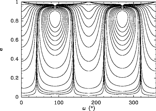
Figure 1: Contour plots of the Kozai Hamiltonian (4) in a $(\omega,e)$ space for $H=0.05$

Assuming zero eccentricity for the primaries, the secular motion of the particle is characterized, to quadrupolar approximation (expansion of the secular Hamiltonian to $2^{\mathrm{nd}}$ order in powers of the semi-major axis ratio) by the following constants of motions (Kinoshita & Nakai 1999; Krymolowski & Mazeh 1999; Ford et al. 2000; Beust & Dutrey 2006)

$$F = (2+3e^{2})(3\cos^{2}i-1)+15e^{2}\sin^{2}i\cos 2\omega$$ (2)

$$H = (1-e^{2})\cos^{2}i\qquad,$$ (3)

where $e$ stands for orbital the eccentricity of the particle, $i$ for its inclination with respect to the orbital plane of the primaries and $\omega$ for the particle’s argument of periastron relative to this plane. The first constant ($F$) is the reduced Hamiltonian itself and $H$ is the reduced vertical component of the angular momentum which is a secular constant thanks to the axial symmetry of the averaged problem. Combining both we can eliminate the inclination

$$F=(2+3e^{2})\left(\frac{3H}{1-e^{2}}-1\right)+15e^{2}\left(1-\frac{H}{1-e^{2}}\right)\cos 2\omega$$ (4)

Contour plots of this expression in $(\omega,e)$ space for a given $H$ value are called Kozai diagrams. The Kozai mechanism regime is characterized by small values of $H$ (high initial inclinations). Figure 1 shows such a diagram corresponding to $H=0.05$. We note the two islands of libration around $\omega=90\degr$ and $\omega=270\degr$ (or $-90\degr$) characteristic for Kozai resonance. In a pure 3-body Newtonian dynamics, the particle just secularly moves along one of these curves. It is then obvious to see that its evolution is characterized by strong periodic eccentricity increases. In the same time $e$ increases, $i$ decreases to keep $H$ constant. If for a given particle $\omega$ librates around $\pm 90\degr$, it is said to be trapped in Kozai resonance. But even if $\omega$ circulates, its evolution is characterized by the same eccentricity / inclination modulation described above, the maximum $e$ values being reached when $\omega=\pm 90\degr$.

As quoted above, this regime is valid for small $H$ values. If the particle has initial zero eccentricity, it can be shown analytically (Kinoshita & Nakai 1999) that the minimum inclination required for Kozai mechanism to start is $\arccos(\sqrt{3/5})\simeq 39.23\degr$. Alternatively, it can operate at smaller inclination if the initial eccentricity is larger. But a some point in the secular evolution, it will reach an inclination above this threshold.

This dynamical mechanism is also active in hierarchical triple systems (Harrington 1968; Söderhjelm 1982; Eggleton et al. 1998; Krymolowski & Mazeh 1999; Ford et al. 2000), the inner orbit being subject to a similar evolution under secular perturbations by the outer body. This is particularly relevant for triple systems because they are often non-coplanar. Similarly, it is expected to be active on planetary orbits in binary star systems, as soon as the orbit of the planets are significantly non coplanar with that of the binary ($i\ga 40\degr$, see above). This can affect the stability of the planetary orbits, especially if several planets are present (Innanen et al. 1997; Malmberg et al. 2007). It was actually invoked to explain the high eccentricity of some extrasolar planets in binary systems (Holman et al. 1997; Libert & Tsiganis 2009).

2.2 Kozai migration

This mechanism could also apply to the GJ 436 case, as a way to sustain the eccentricity of GJ 436b. But tides inevitably lead to a circularization within the standard timescale (see simulations below and also application to the TyCra system in Beust et al. 1997).

To render Kozai mechanism active despite the presence of tides, one must lower the strength of the tides. This can be done assuming a higher $Q_{p}$ as suggested by Mardling (2008) (see Introduction), but this is even not enough. Even with an arbitrary large $Q_{p}$, there is still forced apsidal precession due to the planetary and stellar quadrupole moments and to General Relativity (see Sect. 3). With the present day semi-major axis of GJ 436b, this is enough to override the Kozai mechanism.

Then only way to damp all these effects to allow the onset of Kozai cycles is to assume a larger semi-major axis for the planet during a first evolutionary phase. The purpose of the present paper is to investigate this idea. Of course, the present orbital semi-major axis of GJ 436b is well constrained from radial-velocity monitoring, but our idea is to suggest that it used to be larger in the past, typically 5–10 times larger than today. In this context, all perturbing effects listed are too weak to prevent the onset of Kozai cycles. Then when the eccentricity increases, the periastron drops, because as long as tides are not active, the semi-major axis remains a secular invariant. Hence tidal friction starts at periastron. This leads to a gradual decrease of the orbit (i.e., the semi-major axis) which causes it to shrink and to finally reach its present location. This process is called Kozai migration. It has been described by Eggleton & Kiseleva-Eggleton (2001); Wu & Murray (2003) and more recently by Fabrycky & Tremaine (2007). It is viewed today as one of the various migration mechanism that can act in planetary systems. Our aim is to investigate this scenario in the context of GJ 436b. We show that although it cannot prevent the final circularization of the planet, under suitable assumptions it can considerably slow down the circularization process, thus explaining how the eccentricity of GJ 436b could still be significant a few Gyrs after the formation of the system in spite of strong tidal friction.

3 Tidal forces and $N$-body integration

3.1 Basic tidal forces

Our goal is to test the scenario of Kozai migration to the GJ 436b case. This needs to be done via numerical integration. The various tidal forces are described in Mardling & Lin (2002). We recall briefly this theory here. Let us consider i) a star with mass $m_{s}$, radius $R_{s}$, an apsidal constant $k_{s}$ and a dissipation parameter $Q_{s}$, ii) a planet with mass $m_{p}$, radius $R_{p}$, an apsidal constant $k_{p}$ and a dissipation parameter $Q_{p}$. The tidal forces acting on the planet are

1. the acceleration due to the quadrupole moment of the planet due to the distorsion produced by the presence of the star:

   $$\@vec{\gamma}_{\mathrm{QD,p}} = \frac{R_{p}^{5}\left(1+m_{s}/m_{p}\right)k_{p}}{r^{4}}\left\{\left[5\left(\@vec{\Omega}_{p}\cdot\@vec{u}\right)^{2}-\Omega_{p}^{2}-\frac{12Gm_{s}}{r^{3}}\right]\@vec{u}\right.$$ (5)

   $$\qquad\qquad\qquad\qquad\qquad\left.\rule[-8.53581pt]{0.0pt}{17.07164pt}-2\left(\@vec{\Omega}_{p}\cdot\@vec{u}\right)\@vec{\Omega}_{p}\right\}\;,$$

   where $\@vec{\Omega}_{p}$ is the spin vector of the planet, $r$ is the distance between the planet and the star, and $\@vec{u}=\@vec{r}/r$, a unit vector parallel to the radius vector of the orbit;

2. the acceleration produced by the tidal damping of the planet

   $$\@vec{\gamma}_{\mathrm{TF,p}}=-\frac{6nk_{p}m_{s}}{Q_{p}m_{p}}\,\left(\frac{R_{p}}{a}\right)^{5}\left(\frac{a}{r}\right)^{8}\left[2\left(\@vec{u}\cdot\dot{\@vec{r}}\right)\@vec{u}+\dot{\@vec{r}}-r\@vec{\Omega}_{p}\times\@vec{u}\right],$$ (6)

   where $a$ is the semi-major axis and $n$ the mean motion of the orbit.

Of course we have symmetric accelerations $\@vec{\gamma}_{\mathrm{QD,s}}$ and $\@vec{\gamma}_{\mathrm{TF,s}}$ for the star. We must add to these forces the relativistic post-newtonian acceleration

$$\@vec{\gamma}_{\mathrm{rel}} = -\frac{G\left(m_{p}+m_{s}\right)}{r^{2}c^{2}}\left\{\left[(1+3\eta)\dot{\@vec{r}}\cdot\dot{\@vec{r}}-2(2+\eta)\frac{G\left(m_{p}+m_{s}\right)}{r}\right.\right.$$ (7)

$$\qquad\qquad\qquad\qquad\left.\left.\rule[-14.22636pt]{0.0pt}{28.45274pt}-\frac{3}{2}\eta\dot{r}^{2}\right]\@vec{u}-2(2-\eta)\dot{r}\,\dot{\@vec{r}}\right\}\;,$$

where $\eta=m_{p}m_{s}/(m_{p}+m_{s})^{2}$ and $c$ is the speed of light. Finally, the equation of motion describing the evolution of the orbit of the planet is

$$\ddot{\@vec{r}}=-\frac{G\left(m_{s}+m_{p}\right)}{r^{3}}\,\@vec{r}+\gamma_{\mathrm{rel}}+\@vec{\gamma}_{\mathrm{QD,p}}+\@vec{\gamma}_{\mathrm{TF,p}}+\@vec{\gamma}_{\mathrm{QD,s}}+\@vec{\gamma}_{\mathrm{TF,s}}$$ (8)

We must also add an equation governing the evolution of the spin vectors. For the planet we have (Mardling & Lin 2002)

$$I_{p}\dot{\@vec{\Omega}_{p}}=-\frac{m_{s}m_{p}}{m_{s}+m_{p}}\,\@vec{r}\times\left(\@vec{\gamma}_{\mathrm{QD,p}}+\@vec{\gamma}_{\mathrm{TF,p}}\right)\quad,$$ (9)

and a symmetric equation for $\dot{\@vec{\Omega}_{s}}$. Note that we typically have $\gamma_{\mathrm{QD,s}}\ll\gamma_{\mathrm{QD,p}}$ and $\gamma_{\mathrm{TF,s}}\ll\gamma_{\mathrm{TF,p}}$ by a factor $m_{p}/m_{s}$, showing that the star itself is very little affected. To lowest order for a synchronized planet, we have $\gamma_{\mathrm{QD,p}}/\gamma_{\mathrm{TF,p}}\simeq 11Q_{p}/6$. With $Q_{p}\ga 10^{5}$. We see that $\gamma_{\mathrm{QD,p}}$ dominates the orbital evolution. However, $\gamma_{\mathrm{TF,p}}$ (the damping term) is responsible for the circularization and must be retained. Also, we have to lowest order

$$\frac{\gamma_{\mathrm{rel}}}{\gamma_{\mathrm{QD,p}}}\simeq\frac{3}{11k_{p}}\frac{\dot{\@vec{r}}\cdot\dot{\@vec{r}}}{c^{2}}\frac{r^{5}}{R_{p}^{5}}\frac{m_{p}}{m_{s}}$$ (10)

With the numerical values for the parameters of GJ 436b quoted in Mardling (2008), this ratio is $\simeq 1.6$. This shows that relativistic effects are expected to be comparable to tides and must not be neglected. However, as pointed out by Mardling & Lin (2002), the only secular effect of the relativistic potential is to produce an apsidal advance. This also holds for $\@vec{\gamma}_{\mathrm{QD,p}}$ as both effects are conservative. They do not affect the circularization process due to $\@vec{\gamma}_{\mathrm{TF,p}}$.

3.2 Inclusion into $N$-body integration and averaging

As we want to investigate the combined effect of tides and planetary perturbations, these forces must be included into a $N$-body integration scheme. Our basic scenario is an inner planet (GJ 436b) subject to tidal interaction from the star, and perturbed by an outer, inclined and more massive planet (with mass $m^{\prime}$ and semi-major axis $a^{\prime}$) that is itself not subject to tides.

A major difficulty is that we have to deal with phenomena with very different timescales. In the context of GJ 436, the period of Kozai cycles is typically $\sim 10^{5}\,$yr, while the tidal circularization acts on timescales $\ga 10^{8}\,$yr. Hence an efficient $N$-body integrator is required.

A standard way to overcome this difficulty is to average all interaction terms over the orbital motions of both bodies. This can concern the interaction 3-body Hamiltonian between the planet and the perturber, as well as the tidal terms. This way only the secular part of the perturbations is retained.

The averaging of the tides and of the relativistic terms is done only over the orbital period of the inner planet. To do this, it is convenient to derive the effect of the tides on the specific angular momentum vector $\@vec{h}=\@vec{r}\times\dot{\@vec{r}}$ and the Runge-Lenz vector (Mardling & Lin 2002; Fabrycky & Tremaine 2007; Eggleton & Kiseleva-Eggleton 2001)

$$\@vec{e}=\frac{\dot{\@vec{r}}\times\@vec{h}}{G\left(m_{s}+m_{p}\right)}-\@vec{u}\qquad.$$ (11)

Each additional acceleration $\@vec{\gamma}$ will induce a rate of change of $\@vec{e}$ and $\@vec{h}$ given by

$$\frac{\mathrm{d}\@vec{h}}{\mathrm{d}t}=\@vec{r}\times\@vec{\gamma}\quad;\quad\frac{\mathrm{d}\@vec{e}}{\mathrm{d}t}=\frac{2\left(\@vec{\gamma}\cdot\dot{\@vec{r}}\right)\@vec{r}-\left(\@vec{r}\cdot\dot{\@vec{r}}\right)\@vec{\gamma}-\left(\@vec{\gamma}\cdot\dot{\@vec{r}}\right)\dot{\@vec{r}}}{G\left(m_{s}+m_{p}\right)\quad.}$$ (12)

These equations are then averaged over the orbital period of the inner planet. Using Hansen coefficients, this can be done in closed form. Explicit formulas are given by Mardling & Lin (2002).

The averaging of the interaction Hamiltonian with the outer perturber over the orbital period of both bodies is more complex, as this cannot be done in closed form. One has to expand the corresponding terms in ascending powers of the semi-major axis ratio $a/a^{\prime}$ between the planet and the perturber (using Legendre polynomials). Assuming $a/a^{\prime}\ll 1$, it is truncated to some given order and then averaged over both orbits. Wu & Murray (2003) and Fabrycky & Tremaine (2007) truncate the Hamiltonian to second order (quadrupolar), while Ford et al. (2000) recommend third order (octupolar). Mardling & Lin (2002) give explicit formulas up to third order (for coplanar orbits though). As explained below, the level of accuracy required by our study forced us retain terms up to 4^th order in $a/a^{\prime}$, i.e. one level beyond octupolar. We used Maple to derive analytic formulas up to this level.

Another way to handle the 3-body interaction is to use symplectic integration. The main difficulty is to combine it with tidal forces. The theory of symplectic integration is based on the Hamilton equations of motion that apply to any $N$-body problem. Its background is for instance described in Saha & Tremaine (1992) and Chambers (1999). The key idea is to split the Hamiltonian $H$ into pieces, say $H=H_{A}+H_{B}$, each of them being exactly integrable, and then to integrate each part separately alternatively. Most common symplectic integrators (Chambers 1999; Levison & Duncan 1994) are based on the following second order scheme: At each time-step $\tau$, we must

1. advance $H_{B}$ by a half step $\tau/2$;

2. advance $H_{A}$ for the full time step $\tau$;

3. Re-advance $H_{B}$ by $\tau/2$.

In planetary and hierarchical $N$-body problems, $H_{A}$ corresponds typically to a collection of independent Keplerian Hamiltonians and $H_{B}$ to the disturbing function. We will name this scheme $B(\tau/2)A(\tau)B(\tau/2)$. Our goal here is to include tides to it, i.e. dissipative forces. Of course with dissipation the integration, as well as the real problem, is no longer symplectic. This does not prevent the integration method from being efficient, at least for the $N$-body forces. Typically, with the second order scheme described above, a time-step of $\sim 1/20$ of the smallest orbital period is enough in standard problems to ensure a conservation of the energy to $\sim 10^{-6}$ relative level (Beust 2003). Including dissipative forces leads to a non preservation of the energy, but the same time-step can be kept. There have been actually many successful attempts in recent years to include dissipative forces into symplectic integrators (Malhotra 1994; Kehoe et al. 2003; Ćuk & Burns 2004; Marzari & Weidenschilling 2006).

The most straightforward way to proceed is to include the integration of the various forces given above into the $B(\tau/2)$ sub-steps (the disturbing part of the integration). However this turns out not to be efficient in our case. The reason is that the tidal forces are highly dependant on the distance $r$ between the planet and the star ($\propto r^{-4}$ and even steeper). Therefore, when considering significantly eccentric orbits, keeping the standard symplectic time-step leads to an insufficient mapping of the tidal forces close to periastron.

To overcome this difficulty, we used averaged formulas only for the tidal and relativistic terms. Then we add to our symplectic scheme two sub-steps $T(\tau/2)$ of integration of these averaged equations for $\@vec{e}$ and $\@vec{h}$, in the order $B(\tau/2)T(\tau/2)A(\tau)T(\tau/2)B(\tau/2)$:

1. advance $H_{B}$ by a half step $\tau/2$;

2. integrate the averaged tidal equations by $\tau/2$;

3. advance $H_{A}$ for the full time step $\tau$;

4. re-integrate the averaged tidal equations by $\tau/2$;

5. re-advance $H_{B}$ by $\tau/2$.

At each $T(\tau/2)$ sub-step, we integrate simultaneously the evolution of the spin vectors of the bodies via Eq. (9). The advantage of this approach is that it avoids the use of truncated expansions, while still being efficient. We modified this way our symplectic integrator HJS dedicated to hierarchical systems (Beust 2003). All computations presented in Sect. 4 have been done using this integrator. Its use is nevertheless more computing time consuming than a fully averaged integrator. This is why we also built a fully averaged integrator for our parametric study (Sect. 5).

To check the validity of our integration method, we also made some comparisons with integrations performed with a conventional Bulirsh & Stoer integrator. Of course the latter integrations were much more time consuming so that they were done over a much less extended time-span. In all cases the agreement appeared excellent. An example is shown on Fig. 3 (eccentricity plot) where we have overplotted in red the result of the conventional integration. Both curves are almost identical, so that the red curve barely appears under the black one.

4 Application to Gliese 436

4.1 Integration starting from the present state

Figure 2: Secular evolution of the eccentricity of GJ 436b starting from the present-day orbit and assuming a standard perturber ($m^{\prime}=0.1M_{\mathrm{Jup}}$, $T^{\prime}=10\,$yr) in different conditions (see text): (a) perturbing planet, but no tides nor relativity; (b) tides and relativity but no perturbing planet; (c) perturbing planet, relativity but no tides, (d) perturbing planet, relativity and tides.

The first element we want to test is how planetary perturbations may affect the present orbit of GJ 436b. As mentioned above, given the present semi-major axis $a=0.0287\,$AU, tides are expected to dominate the dynamical evolution. We therefore performed four runs starting from the present-day orbital configuration with different assumptions:

• run (a): with a distant perturber, but not taking into account the tides nor the general relativistic post-newtonian correction (hereafter GR), i.e. using the standard HJS code;

• run (b): taking into account tides and GR, but with no perturbing planet (run (b) in Fig. 2);

• run (c): with the same perturbing planet as in run (a), but taking now into account the relativistic post-newtonian correction, but no tides;

• run (d) : with the same planet taking into account both GR and tides.

In all cases, the perturbing planet was chosen with mass $m^{\prime}=0.1\,M_{\mathrm{Jup}}$ and semi-major axis $a^{\prime}=3.583\,$AU (i.e., with orbital period $T^{\prime}=10\,$yr) as a typical convenient set of parameters (see Sect. 5), compatible with the constraints of Montagnier et al. (2012) based on radial velocity residuals and photometry. In addition we fix the initial tilt angle $i_{0}$ between the two orbits to $75\degr$ to be able to generate a strong Kozai resonance. We assume the stellar, planetary and tidal parameters given by Mardling (2008) and listed in the Introduction.

In Fig. 2 we show the secular evolution of the eccentricity of GJ 436b over $2\times 10^{7}$ yr in the four cases. In case (a), we see as expected a large amplitude modulation characteristic for the Kozai resonance created by the perturbing planet. In case (b), we note a gradual circularization with a time-scale $\simeq 2\times 10^{8}$ yr. In case (c) (same as (a) but with GR taken into account), there is no Kozai resonance anymore. The relativistic precession actually smoothes the Kozai mechanism. The eccentricity is basically constant with high frequency, small amplitude oscillations. In run (d) (with tides and relativity), the high frequency oscillation is superimposed to a tidal decrease at the same rate as in case (b). The main conclusion we can derive from these runs is that the perturbing planet could in principle induce a strong Kozai resonance, but that tides and GR override this effect. Even GR alone (run (c)) is enough to cancel out the Kozai resonance. The reason is that the secular precession induced by GR is larger than that induced by the Kozai resonance. As shown by Fabrycky & Tremaine (2007), GR adds an extra term to the secular precession of the argument of periastron $\omega$, and subsequently, the maximum eccentricity of the Kozai cycles is significantly reduced. This can be understood considering Eq. (4). With an extra precession for $\omega$, the $\cos 2\omega$ term in the averaged Hamiltonian $F$ can be considered as rapidly varying, so that it secularly averages to zero. Only the first term can be kept in $F$. This makes the Hamiltonian independent of all angles, making all related actions constant, and hence $e$ and $i$ are constant. This is what we get here.

If we consider the dissipative case with tides, the net result in our case is that the tidal circularization process remains almost unchanged (run (d)) with respect to the case with no perturbing planet (run (b)).

The Kozai resonance appears thus unable to sustain the high present eccentricity of GJ 436b over the age of the system. The only ways to solve this paradigm are either to increase the strength of the Kozai resonance either to lower the tides and the relativistic effects. The former way would imply to increase the mass of the perturbing planet by at least two orders of magnitude; this would render it incompatible with the constraints of Montagnier et al. (2012). The latter way can be achieved assuming a larger semi-major axis for GJ 436b. Of course the present semi-major axis is well constrained, but we may assume that it used to be larger in the past. This is why we come to the idea of Kozai migration.

4.2 The Kozai migration scenario

4.2.1 General description

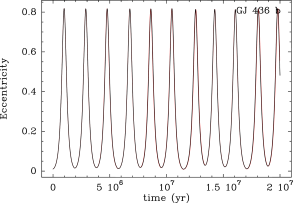
Figure 3: Secular evolution over $2\times 10^{7}\;$yr of GJ 436b assuming an initial value $a=0.287\,$AU and a perturber with $m^{\prime}=0.1M_{\mathrm{Jup}}$ and $a^{\prime}=3.583AU$ ($T^{\prime}=10\;$yr): Eccentricity (top left), semi-major axis (top right), rotation speed with respect to the orbital mean-motion ($\Omega/n$, bottom left), and obliquity angle (bottom right). On the eccentricity plot we overplot in red the result of the same integration, but using a conventional Bulirsh & Stoer integrator

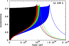
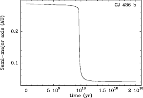
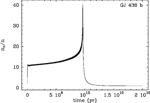
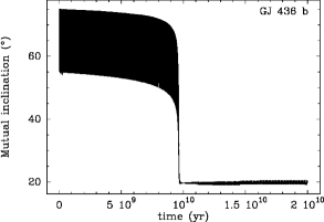
Figure 4: Same evolution as in Fig. 3, but over $2\times 10^{10}\;$yr: Eccentricity (top left), semi-major axis (top right), rotation speed with respect to the orbital mean-motion ($\Omega/n$, bottom left), mutual inclination between the two orbits (bottom right). On all plots, the black curve corresponds to our symplectic integration. The color curves on the eccentricity plot are calculated with a fully averaged integrator, with interaction Hamiltonian truncated up to various orders: 2^nd order (blue), 3^rd order (green), and 4^th order (red).

We describe now into details a typical run where we assume an initial semi-major axis for GJ 436b significantly larger than the present value, and where both GR and tides are taken into account, with unchanged tidal parameters with respect to Sect. 4.1. We assume for the perturber the same parameters as in Sect. 4.1 ($a^{\prime}=3.583\,$AU, $m^{\prime}=0.1\,M_{\mathrm{Jup}}$, $i_{0}=75\degr$), but we take as initial semi-major axis for GJ 436b $a_{0}=0.287\,$AU (i.e, 10 times its present-day value).

Fig. 3 shows the secular evolution of GJ 436b in this context over $2\times 10^{7}\,$yr. We see that the eccentricity is subject to a large amplitude modulation characteristic for Kozai resonance. With $a_{0}=0.287\,$AU, apsidal precession arising from GR and tides is no longer able to override the Kozai resonance. But at peak eccentricity ($e\simeq 0.8$) in the Kozai cycles, the periastron drops to 0.05–0.06 AU, i.e., only twice the present-day semi-major axis. As a result, tides are at work in peak eccentricity phases. This can be seen in Fig. 3. We note a rapid reduction of the obliquity of GJ 436b relative to its orbital plane (initially fixed to $30\degr$), so that after a few $10^{7}\,$yr, the spin axis of GJ 436b remains perpendicular to its orbital plane. We also note a spinning up of the planet’s rotation. On Fig. 3 (bottom-left), we plot as a function of time the ratio of the rotation velocity GJ 436b to its orbital mean-motion ($\Omega/n$), so that 1 means synchronism. This ratio was initially fixed to 2, and we note a gradual increase up to 10 at $t=2\times 10^{7}\,$yr. This reveals a spinning up of the planet, as the orbital mean-motion (i.e. the semi-major axis) is not subject to so drastic changes in the same time. Finally, we note a very small decrease of the semi-major axis over the time-span considered. These effects are clearly due to the tides at work in high eccentricity phases. This shows up obviously in the staircase-like shape of the temporal evolution of the parameters displayed. Actually they are subject to some evolution only in the peak eccentricity phases, and remain unchanged inbetween. The spinning up of the planet is also a consequence of the tides in high eccentricity phases. The rotation of GJ 436b tries indeed to tidally synchronize with the orbital angular velocity at periastron, which is very different from the mean-motion due to the high eccentricity. With a peak eccentricity of $\sim 0.8$, synchronism with angular velocity at periastron means actually $\Omega/n\simeq 16$. Finally, the semi-major axis decrease reveals a loss of orbital energy due to tidal friction.

We come now to describing the same simulation, but over a much longer time span, i.e. 20 Gyrs (Fig. 4). This timescale is intentionally taken larger than the age of the system and even of the Universe to show the possible future evolution. We display as in Fig. 3 the eccentricity, the semi-major axis, the $\Omega/n$ ratio, and the mutual inclination between the two orbits. On the eccentricity plot, the color curves are calculated using various averaged integrators (see below). The one corresponding to our symplectic integration in the black one. We clearly see a two-fold evolution, first before 10 Gyrs and then after. In the first phase, Kozai resonance is still active as can be seen from the high amplitude eccentricity oscillations. In the same time, the semi-major axis is subject to a slight decrease. The eccentricity oscillations do not remain identical though. Actually the peak eccentricity slightly increases but a more striking fact is that the bottom eccentricity of the Kozai cycles gradually increases to finally reach the peak eccentricity after $\sim 10\,$Gyr. At this point (beginning of the second phase) the eccentricity oscillations stop, which means that the GJ 436b gets out of the Kozai resonance. The semi-major axis drops then much more quickly and the eccentricity decreases to zero within a few extra Gyrs. During almost all the evolution (apart from the beginning), the rotation of GJ 436b remains synchronized with the angular velocity at periastron in high eccentricity phases. The increase of $\Omega/n$ during the first phase is related to the gradual increase of the peak eccentricity. In the second phase $\Omega/n$ gradually decreases towards 1. At the end of the simulation, GJ 436b is tidally synchronized and circularized, but the final semi-major axis is several times smaller than the initial one. The Kozai migration is ended.

This two-fold behaviour in Kozai migration process was already noted by Wu & Murray (2003) and Fabrycky & Tremaine (2007). Actually our results of Fig. 4 are very similar to the corresponding ones of Fabrycky & Tremaine (2007).

4.2.2 The first phase

During the first phase, the planet still undergoes Kozai oscillations, but the bottom eccentricity of the cycles gradually increases to finally reach the peak one. This can be explained by a shift in Kozai diagram.

In a pure 3-body Newtonian dynamics, the planet just secularly moves along one of the level curves in a Kozai diagram similar to that of Fig. 1. In the $\omega$-circulating case, the curves are explored from left to right with $\mathrm{d}\omega/\mathrm{d}t>0$, and in the $\omega$-librating case (the genuine “resonant” orbits), the curves are explored clockwise around the stable point. Now, both GR and tides add an extra, positive component to $\mathrm{d}\omega/\mathrm{d}t$ (Fabrycky & Tremaine 2007) at peak eccentricity in the cycles. This results in a slight shift towards right in the Kozai diagram each time the planet passes through a peak eccentricity phase. The planet jumps to another nearby curve located to the right. It is then obvious to see from Fig. 1 that this change induces a decrease of the bottom eccentricity in the $\omega$-librating case and an increase in the $\omega$-circulating case. Now it is also obvious that thanks to these shifts in diagram at each eccentricity peak, a planet initially in the $\omega$-librating case will be pushed to move to $\omega$-circulating after a while. Consequently the bottom eccentricity of the planet is expected to eventually first decrease during the $\omega$-librating phase and then to further increase in the subsequent $\omega$-circulating regime. This is exactly what is reported by Fabrycky & Tremaine (2007) in their Fig. 1. After a short decrease, the bottom eccentricity of the cycles increases gradually to 1. In our Fig. 4, we see that the bottom eccentricity (black curve) of the cycles does not immediately start to increase, but we do not see an initial decrease like in Fabrycky & Tremaine (2007). In fact, the more realistic integration is actually ours. The reason is that the integration of Fabrycky & Tremaine (2007) was made on the basis of a quadrupolar expansion of the Hamiltonian, as well as the Kozai diagram in Fig. 1. It is thus not surprising to see them in perfect agreement. But our integration, made using a symplectic integrator, is not truncated and is accurate to any order in $a/a^{\prime}$. Ford et al. (2000) showed that retaining higher order terms, in particular up to the octupolar level (3^rd order in expansion in $a/a^{\prime}$) considerably improves the accuracy of the integration, especially in the vicinity of the separatrix between the two regimes, which is the case discussed here.

In any case, when the planet enters the $\omega$-circulating regime, the bottom eccentricity of the cycles is forced to increase.

4.2.3 The second phase and the link with the Batygin et al. (2009) model

When the bottom eccentricity reaches the peak one, then the planet moves along a more or less straight line in the Kozai diagram. Tides and GR are now active permanently as the eccentricity is permanently high. This causes the precession of $\omega$ to increase. This forces the planet to start a more sharp tidal decrease that makes it get out of the Kozai resonance. In this second phase, the planet gets gradually tidally circularized.

An important outcome of this scenario is that it can provide a solution to the eccentricity paradox of GJ 436b. We note in Fig. 4 that the first phase of the secular evolution lasts several Gyrs. Hence GJ 436b may have first spent a long time in the first phase before starting a sharp tidal decrease. Moreover, we note that in the second phase, even if the semi-major axis shrinks quickly, it still takes a few more Gyrs to the eccentricity to decrease downto zero. This could appear surprising, as we are now away from Kozai resonance. In Fig. 4, the situation of the planet at $\sim 13\,$Gyrs is similar to the one we studied in Fig. 2. In the latter case, the eccentricity of GJ 436b decreases downto zero in $\sim 2\times 10^{8}\,$yr, but in Fig. 4 it still takes a much longer time from 13 Gyrs to reach zero. How could we explain this discrepancy ?

The difference comes from the dynamical configuration of the 3-body system. It is in fact closely related to the quasi-stationary solution described by Batygin et al. (2009). Batygin et al. (2009) studied the coplanar 3-body system. They showed that there exist two apsidal fixed points in this system, characterized by $\mathrm{d}e/\mathrm{d}t=0$, and $\varpi-\varpi^{\prime}=0$ or $\varpi-\varpi^{\prime}=\pi$, where $\varpi$ and $\varpi^{\prime}$ are the longitude of periastron of GJ 436b and the perturber respectively. There is always one stable point among these two configurations around which librations can occur. In that case, $\varpi-\varpi^{\prime}$ just librates around its equilibrium value, and $\mathrm{d}e/\mathrm{d}t=0$ periodically vanishes. As a result, the decrease of the eccentricity is much slower. Batygin et al. (2009) showed that adding tides to this peculiar system considerably increases the tidal circularization time, because the angular momentum transfer associated with tidal dissipation is now shared among the two interacting orbits. This is of course a peculiar situation, but as mentioned above, these points tend to behave as attractors.

The situation we describe here differs from that of Batygin et al. (2009) because we do not have a coplanar configuration. But the starting point of the second phase is also characterized by a stationary point with $\mathrm{d}e/\mathrm{d}t=0$. At the end of the first phase (Kozai cycles), when the bottom eccentricity of the cycles equals the peak one, GJ 436b moves along a straight line in the Kozai diagram. Hence we have $\mathrm{d}e/\mathrm{d}t=0$. Contrary to Batygin et al. (2009), here $\varpi-\varpi^{\prime}$ circulates during the second phase. The reason is that in the coplanar problem, there is no quadruplar component to $\mathrm{d}e/\mathrm{d}t$. The expression of $\mathrm{d}e/\mathrm{d}t$ given by Batygin et al. (2009) arises indeed from the octupolar expansion. But at high inclination, the quadrupolar component to $\mathrm{d}e/\mathrm{d}t$ dominates, so that the constraints are different. But the common feature is that the starting point of both evolutions is characterized by a stationary point in eccentricity in the pure secular 3-body evolution. The result is a huge increase of the tidal circularization time by a factor 50 at least, like in the evolution described by Batygin et al. (2009). Besides, the apsidal alignment criterion could be used as a diagnostic. If an apsidally aligned companion is discovered in the future in the radial velocity residuals of the star, it would be a strong indication in favor of a coplanar configuration like described by Batygin et al. (2009); conversely if this is not the case, the companion could be considered as highly inclined with good probability.

5 Exploration of the parameter space

5.1 Description of the results

We claim that the Kozai migration process we describe could fit the present day configuration of the GJ 436 system. GJ 436b could fairly well be today in the middle of the second phase, with an already reduced semi-major axis and a slowly decreasing eccentricity. In Fig. 4, the situation of the planet at $\sim 13\,$Gyrs can be compared to the present day orbital configuration of GJ 436b.

Of course 13 Gyrs is too long compared to the age of the GJ 436 system. But the timescale of the two-fold evolution can vary considerably depending on the initial parameters of the model, so that adjusting them to fit to any given age less than the age of the Universe is possible.

We come now to exploring the parameter space of this scenario to try to derive in which case it can be compatible with the observation. We tested various orbital configurations, exploring the parameter space. The important parameters are

• the mass $m^{\prime}$ and semi-major axis $a^{\prime}$ (or equivalently the orbital period $T^{\prime}$) of the perturber;

• the initial semi-major axis $a_{0}$ of GJ 436b;

• the initial mutual inclination $i_{0}$ between the two orbits.

Note that instead of $i_{0}$, the actual critical parameter is the reduced vertical component of the specific angular momentum $h=\sqrt{1-e^{2}}\,\cos i$, which is a secular constant of motion (See Sect. 2.1). But in all our simulations we took an initial eccentricity $e_{0}=0.01$ for GJ 436b, so that $h$ is unambiguously related to $i_{0}$.

Other parameters such as the eccentricity of the perturber, the initial rotation speed and rotation axis orientation of GJ 436b turned out to have only a minor influence on the global behaviour of the system, so that exploring the space of the major parameters is enough for our purpose. In particular, in all the following, the initial eccentricity $e^{\prime}$ of the perturber was set to $0.03$ as a typical standard value.

The key outcome to monitor is the transition time between the two phases in the scenario (hereafter $t_{\mathrm{tr}}$), which occurs close to 10 Gyrs in Fig. 4. This timescale appeared to be extremely sensitive to the parameters, ranging from less than $10^{5}\,$yr in some extreme cases to hundreds of Gyrs in other configurations. In all cases, most of the orbital decrease and circularization that occurs after $t_{\mathrm{tr}}$ is achieved with $\sim 1.5t_{\mathrm{tr}}$.

In our exploration, we consider as likely any $t_{\mathrm{tr}}$ value between 1 Gyr and 10 Gyr. Shorter values are not compatible with a not yet circularized GJ 436b today, and with longer values, the star is not old enough to have entered the second phase yet. Our goal was to derive which sets of parameters yield a convenient $t_{r}$. To do this, we first used our symplectic code in a few cases, and then our averaged integrator to save computing time. As mentioned above, the averaging process of the Hamiltonian due to the perturber cannot be done in closed form. One has to first expand it in ascending powers of $a/a^{\prime}$, to truncate it to some given order and then average over both orbits. Fabrycky & Tremaine (2007) truncate to second order (quadrupolar), while Ford et al. (2000) recommends third order (octupolar). We checked that being in correct agreement with the symplectic integration (in particular in the monitoring of $t_{\mathrm{tr}}$ which is a very sensitive parameter) requires to retain terms up to 4^th order in $a/a^{\prime}$, i.e. one level beyond octupolar. The use of a truncated integrator does not change the global two-fold behaviour reported above, but it affects its timescale. This is illustrated in Fig. 4a (eccentricity plot) where we have superimposed to our symplectic integration (black curve) the same eccentricity evolution, but calculated with averaged integrators truncated at various orders: second (blue), third (green) and 4^th (red). The use of the quadrupolar truncation generally leads to an error on $t_{\mathrm{tr}}$ of $\sim 50\%$. Most of the time it overestimates it. This can be understood easily: In a pure Newtonian dynamics (no tides, no relativity, such as in Fig. 2a), all Kozai cycles are strictly identical in the quadrupolar approximation. The motion is strictly periodic, as can be seen from Fig. 1. This is due to the absence of the perturber’s eccentricity and argument of periastron in the interaction Hamiltonian (Eq. (2)). This is no longer true at higher order, as shown by Krymolowski & Mazeh (1999); Ford et al. (2000). Due to secular changes of the perturber’s orbit, the Kozai cycles are no longer identical (see Fig. 3a for instance). The total number of Kozai cycles achieved within a given (long) time-span can thus vary depending on the theory assumed. As the efficiency of the Kozai migration process depends on the integrated number of peak eccentricity phases reached, this explains the variability of $t_{\mathrm{tr}}$. We see from Fig. 4a that the use of a third order (octupolar) theory (green curve) considerably enhances the agreement with the symplectic integration. A $\sim 5$% agreement is reached if we go to 4^th order (red curve). Or course better agreement could be reached if we used even higher order formulas. But in that case, the averaged formulas are so complex that the gain in computing time with respect to the symplectic integration is small. As a 5% accuracy on $t_{\mathrm{tr}}$ is enough for our analysis, we decided to use 4^th order theory.

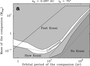
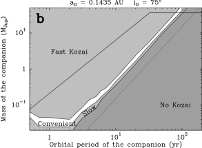
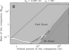
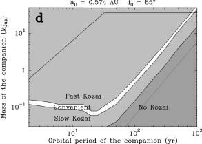
Figure 5: Result of the exploration of the parameter space for four $(a_{0},i_{0})$ combinations. a: $a_{0}=0.287\,$AU, $i_{0}=75\degr$; b: $a_{0}=0.1435\,$AU, $i_{0}=75\degr$; c: $a_{0}=0.287\,$AU, $i_{0}=85\degr$; d: $a_{0}=0.574\,$AU, $i_{0}=85\degr$. In each plot, the upper observational limits (radial velocities and imaging) are represented as a solid line; the oblique dotted line corresponds to the limit $t_{\mathrm{GR}}=t_{\mathrm{Kozai}}$ as given by Matsumura et al. (2009).In the upper left plot, the dashed lined are $m^{\prime}\propto T^{\prime}{-1/3}$ and $m^{\prime}\propto T^{\prime}{{}^{2}}$ power laws (see text).

Figure 5 shows a summary of the result of this exploration of the parameter space. Each plot corresponds to the use of a fixed set of values ($a_{0},i_{0}$) where we let the other parameters $(T^{\prime},m^{\prime})$ vary. According to the simulation results, we divide the $(T^{\prime},m^{\prime})$ plane into different regions depending on the resulting value of $t_{\mathrm{tr}}$. Regions marked “Fast Kozai” correspond to cases where $t_{\mathrm{tr}}<1\,$Gyr. In these regions, the Kozai migration process should have ended a long time ago, and we would expect GJ 436b to be synchronized and circularized today. This situation logically applies to massive and/or close-in perturbers (top-left parts of the panels), when the disturbing action is stronger and the period of Kozai cycles smaller. Conversely, towards the bottom parts of the panels (small and/or distant perturbers), we have regions marked as “Slow Kozai”, thus corresponding to $t_{\mathrm{tr}}>10\,$Gyr. In such cases, $t_{\mathrm{tr}}$ is just too long to allow GJ 436b to lie in the second phase of the Kozai migration process today. This cannot match the observation, as during the first phase of the evolution (Kozai cycles), the semi-major axis only undergoes a very small decrease an cannot reach the present day value. We also note in some cases regions marked “No Kozai” corresponding to very low mass and distant companions. In such cases, the perturbing action of the companion is so weak that GR (even at the considered distance) is strong enough to prevent the onset of Kozai cycles. Thus GJ 436b’s eccentricity never grows and it can never reach its present-day location. To illustrate this fact, we add to all plots in Fig. 5 an oblique line which corresponds in each case to $t_{\mathrm{GR}}=t_{\mathrm{Kozai}}$, where $t_{\mathrm{GR}}$ and $t_{\mathrm{Kozai}}$ are characteristic times for GR and for Kozai oscillations respectively. These timescales read (Matsumura et al. 2009)

$$t_{\mathrm{GR}} = \frac{Tc^{2}a\left(1-e^{2}\right)}{3G\left(M+m\right)}\qquad,$$ (13)

$$t_{\mathrm{Kozai}} = \frac{2T^{\prime 2}}{3\pi T}\frac{M+m+m^{\prime}}{m^{\prime}}\left(1-e^{\prime 2}\right)^{2}\qquad.$$ (14)

Here we have computed these timescales assuming $e=0$. Note that the real period of the Kozai cycles equals $t_{\mathrm{Kozai}}$ within a factor of order unity (Ford et al. 2000; Beust & Dutrey 2006). It is straightforward to see that $t_{\mathrm{GR}}=t_{\mathrm{Kozai}}$ implies $m^{\prime}\propto T^{\prime 2}$ (with $m^{\prime}\ll M$), hence the oblique dotted lines in Fig. 5. No Kozai oscillations are to be expected below this limit ($t_{\mathrm{GR}}<t_{\mathrm{Kozai}}$), which is confirmed by our numerical exploration. The “No Kozai” regions extend indeed somewhat above the dotted lines the our plots. This is due to the higher order effects that are not taken into account in the above simple formulas.

In the middle of the fast and slow Kozai regions, a convenient strip appears where the value of $t_{\mathrm{tr}}$ allows GJ 436b to lie presently in the middle of the second phase of the Kozai migration process. Note that for a given set of parameters, the probability of witnessing this phase today is not small, as the second phase lasts typically $\sim 0.5t_{\mathrm{tr}}$.

To all plots in Fig. 5 we superimpose a solid line that corresponds to the observational upper limits of Montagnier et al. (2012) for any additional planet to GJ 436. The left oblique part corresponds to the radial velocity limit and the horizontal upper part to the imaging (adaptive optics) limit. Consequently, any set of $(T^{\prime},m^{\prime})$ values located above this line must be rejected, and for an initial set of parameters ($a_{0},i_{0}$) to be possible, the convenient strip must cross the region below the observational limits. In all plots, the lower $T^{\prime}$ value (in $x$-axis) was set according to the stability limit of the system. Systems with smaller $T^{\prime}$ values are unstable. The stability was tested for these orbits with the unaveraged symplectic integrator. The upper limit in $T^{\prime}$ was set at the point where the convenient strip definitely gets above the observational imaging limit, so that any convenient companion located further away would have been already detected. So, for any given set of initial conditions ($a_{0},i_{0}$), the convenient values for $T^{\prime}$ and $m^{\prime}$ must appear on the plot.

For all displayed cases, the convenient strip appears two-fold. Towards lower $T^{\prime}$ values (close-in perturbers), the convenient $m^{\prime}$ values are a slowly decreasing function of $T^{\prime}$, while for more distant perturbers, they increase rapidly. This can be understood with a careful analysis of the Kozai mechanism. The efficiency of the Kozai migration scenario depends actually on how close GJ 436b can get to the star during the first phase (hence the maximum eccentricity it can reach) and the time it spends at high eccentricity to allow tides to be at work. For close-in perturbers, the process is limited by the maximum eccentricity it can reach. In fact in Fig. 5, close-in perturbers in the convenient strip have masses comparable to that of GJ 436b ($\simeq 0.074M_{\mathrm{Jup}}$), and have semi-major axes only a few times more than GJ 436b initially. Hence the initial angular momentum ratio $l^{\prime}_{0}/l_{0}$ between the perturber and GJ 436b is of order unity or a bit more. Now, due to total angular momentum conservation (we neglect exchanges with spins), we necessarily have

$$l_{0}^{2}+{l^{\prime}_{0}}^{2}+2l_{0}l^{\prime}_{0}\cos i_{0}=l^{2}+l^{\prime 2}+2ll^{\prime}\cos i\qquad,$$ (15)

where $l^{\prime}$ and $l$ stand for the angular momenta of both bodies at peak eccentricity, and $i$ for the mutual inclination in the same phase. Assume now $l^{\prime}=l^{\prime}_{0}$ (the perturber is not affected) and $l=l_{0}\sqrt{1-e^{2}}$ (the semi-major axis is only little affected in the first phase). This equation simplifies to

$$2\frac{l^{\prime}_{0}}{l_{0}}\left(\cos i_{0}-\sqrt{1-e^{2}}\cos i_{0}\right)+e^{2}=0$$ (16)

Solving this equation for $e$ shows that for moderate $l^{\prime}_{0}/l_{0}$ values, the eccentricity cannot go beyond a maximum value that is significantly below 1, while for larger value, any value as close possible to 1 is allowed. In other words, the angular momentum of GJ 436b cannot reach zero because that of the perturber cannot grow to account for the whole angular momentum of the system. Let us assume for instance $i_{0}=75\degr$, $i=30\degr$ (typical values) and $l^{\prime}_{0}/l_{0}=2$. We derive $e\simeq 0.74$, which is high, but significantly below 1 to avoid GJ 436b to be efficiently tidally braked in peak eccentricity phases. The efficiency of the Kozai migration process is therefore limited by the maximum eccentricity value than can be reached, hence by the value of $l^{\prime}_{0}/l_{0}$. Similar $t_{\mathrm{tr}}$ correspond to similar $l^{\prime}_{0}/l_{0}$ values. Assuming now $l^{\prime}_{0}\propto m^{\prime}T^{\prime 1/3}$ and $l_{0}\propto mT^{1/3}$ (low initial eccentricities), a constant $t_{\mathrm{tr}}$ leads $m^{\prime}\propto T^{\prime-1/3}$, hence the decrease of the convenient strip towards close-in perturbers.

For more distant perturbers, the $l^{\prime}_{0}/l_{0}$ ratio is large enough not to limit the peak eccentricity of the Kozai cycles. The efficiency of the process is now limited by the amount of time spent in high eccentricity phases, as tides are only active there. We thus expect $t_{\mathrm{tr}}\propto t_{\mathrm{Kozai}}$, as the longer $t_{\mathrm{tr}}$, the less time is spent within a given time span in high eccentricity phases. As $t_{\mathrm{Kozai}}\propto(M/m^{\prime})\times(T^{\prime 2}/T)$, a fixed value for $t_{\mathrm{tr}}$ will correspond to a constant ratio $T^{\prime 2}/m^{\prime}$. This explains the increase of the convenient strip towards distant perturbers. A more distant perturber just needs to be more massive to generate the same Kozai migration as a closer one.

To illustrate this simple analysis, we have drawn in Fig. 5a two dashed lines corresponding to arbitrary $m^{\prime}\propto T^{\prime-1/3}$ and $m^{\prime}\propto T^{\prime 2}$ power laws. We note that these power laws described above as well followed in the simulations for both regimes, as the convenient strip quite faithfully remains parallel to the dashed lines sketched. To summarize, the convenient strip roughly follows a dual power law regime, with $m^{\prime}\propto T^{\prime-1/3}$ for small $T^{\prime}$ and $m^{\prime}\propto T^{\prime 2}$ for large $T^{\prime}$. Its exact location in ($T^{\prime},m^{\prime}$) space depends on the initial set of parameters ($a_{0},i_{0}$), as can be seen from Fig. 5.

We also note that in all cases, the convenient strip appears quite narrow, although this effect is enhanced on Fig. 5 by the logarithmic scale. In fact, for a given period $T^{\prime}$, Kozai migration is very sensitive to the mass $m^{\prime}$ of the perturber, so that $m^{\prime}$ must assume a well defined value within a factor $\sim 1.5$ to allow $t_{\mathrm{tr}}$ to fall in the right range. However, for a wide range of initial values sets $(a_{0},i_{0})$ (see discussion below), there is a convenient strip in ($T^{\prime},m^{\prime}$) which is compatible with the observational constraints, so that the probability of the scenario is not small.

5.2 Discussion

We come now to compare the location of the convenient strip between various configurations. If we compare Figs. 5a and  5c (same $a_{0}$ but different $i_{0}$), we note that for $i_{0}=85\degr$ the convenient strip is located lower than for $i_{0}=75\degr$. Here again this may be easily understood. With a larger $i_{0}$ the Kozai mechanism is stronger, so that GJ 436b more easily gets a high peak eccentricity and the tides act more efficiently. Hence a less massive perturber is required to achieve the same result.

If we compare configurations with same $i_{0}$ but different $a_{0}$ (Figs. 5a and b on the one hand, and c and d on the other hand) we can see how the convenient strip moves in the ($T^{\prime},m^{\prime}$) diagram if we vary $a_{0}$. We see that increasing $a_{0}$ brings the convenient strip up in the decreasing part of the diagram ($m^{\prime}\propto T^{\prime-1/3}$), and down in the increasing part of the diagram ($m^{\prime}\propto T^{\prime 2}$). If for instance we superimpose Figs. 5a and b, the convenient strip for $a_{0}=0.1435\,$AU falls below that for $a_{0}=0.287\,$AU for small $T^{\prime}$, then crosses it and get above for large $T^{\prime}$. This can be explained. In the decreasing part, the efficiency of the Kozai mechanism is controlled by the angular momentum ratio $l^{\prime}_{0}/l_{0}$. for a larger $a_{0}$, $l_{0}$ is larger and the angular momentum ratio is smaller, so the Kozai mechanism is less efficient. We thus need a larger $l^{\prime}_{0}$ (and hence a larger $m^{\prime}$) to get the same results. This is why the convenient strip is brought up for a larger $a_{0}$. In the increasing part of the diagram, the Kozai mechanism is controlled by $t_{\mathrm{Kozai}}$. As we know that $t_{\mathrm{Kozai}}\propto T^{-1}$, a larger $a_{0}$ leads naturally to a smaller $t_{\mathrm{Kozai}}$ and to a more efficient Kozai migration process. Hence a less massive companion (larger $m^{\prime}$) for the same $T^{\prime}$ is required to achieve the same $t_{\mathrm{Kozai}}$. This is why the convenient strip is brought down if we increase $a_{0}$.

This regime tends nevertheless not to be valid for all values of $a_{0}$. For larger initial orbits, the whole convenient strip is shifted upwards if we increase $a_{0}$. For instance, for $a_{0}=0.574\,$AU and $i_{0}=75\degr$ (configuration not displayed in Fig. 5), the convenient strip is located much higher than with $a_{0}=0.287\,$AU, so that is it barely compatible with the observational constraints. Similarly, with $i_{0}=85\degr$, the convenient strip is shifted upwards for $a_{0}\ga 0.6\,$AU. This behaviour is due to the fact that the efficiency of the tides are related to the minimum periastron reached rather than the maximum eccentricity. As in the first phase, the semi-major axis of GJ 436b is only little affected, for a larger $a_{0}$ a higher eccentricity is necessary to reach the required periastron range.

Now, is it possible to set absolute limits to the unknown parameters ? Setting a lower limit to $i_{0}$ is easy. As described above, if we decrease $i_{0}$ the convenient strip gets higher in ($T^{\prime},m^{\prime}$) space. At some point it crosses the observational limits so that the considered ($a_{0},i_{0}$) must be rejected. We tested several other runs with $i_{0}=65\degr$ and $i_{0}=70\degr$. In all cases the convenient strip (if any) appears above the observational limits. It is then possible to stress that $i_{0}$ must be at least 70–75$\degr$. Note also that the Kozai mechanism is symmetrical with respect to $i_{0}=90\degr$. We checked that runs assuming $i_{0}=95\degr$ and $i_{0}=105\degr$ behave exactly the same way as corresponding runs with $i_{0}=85\degr$ and $i_{0}=75\degr$ respectively. It is thus possible to put an upper limit to $i_{0}$ to 105–110$\degr$. The initial configuration of the system must have been close to perpendicular within less than $20\degr$. This is of course valid for small initial eccentricity $e_{0}$. If $e_{0}$ is high, then $i_{0}$ may take different values. In the general case, a more relevant constraint must be derived for $h=\sqrt{1-e^{2}}\,\cos i$. $70\degr\la i_{0}\la 90\degr$ for small $e_{0}$ means $|h|\la 0.34$, which is valid irrespective of $e_{0}$.

It is also possible to set a lower limit to $a_{0}$. Looking at Fig. 5, we see that for lower $a_{0}$ the convenient strip gets shifted towards left, so that at some point it should cross the radial velocity observational limit. This occurs for $a_{0}\simeq 0.1\,$AU. Hence we can stress that the initial value $a_{0}$ must have been larger.

Giving an upper limit to $a_{0}$ is less easy. We first can notice than choosing a larger $a_{0}$ implies a much more restricted compatible range for $i_{0}$. As noted above, for $i_{0}=75\degr$, $a_{0}=0.287\,$AU is possible, but $a_{0}=0.574\,$AU is barely excluded (too high convenient strip). For $i_{0}=85\degr$ nevertheless, we tested that even fairly large $a_{0}$ values (up $\sim 10\,$AU) we can find a convenient strip in $(T^{\prime},m^{\prime})$ space that falls still below the observational limits. We may thus set an absolute upper limit to $a_{0}\simeq 10\,$AU. However, we must point out that for such values, we are in an extreme Kozai regime with a very high peak eccentricity. Even if such a situation cannot be rejected, whether the onset of such a regime with nearly orthogonal orbits is likely is questionable. Hence even if the absolute compatible range for $a_{0}$ is $0.1$–$10\,$AU, we may stress that the range $0.1$–$0.5\,$AU is more probable.

As pointed out above, in all cases, the convenient strip in $(T^{\prime},m^{\prime})$ space to allow $t_{\mathrm{tr}}$ to fall in the suitable time range is quite narrow. This does not tell that the situation we are describing is improbable, as suitable configurations are possible for a wide range of initial configurations. This tells that for any given set of values $(a_{0},i_{0},T^{\prime})$ the mass of the companion $m^{\prime}$ must fall around a well defined value within a factor $\sim 1.5$. We nevertheless note that taking larger $a_{0}$ values leads to generate narrower convenient strips. This shows up already in Fig. 5d ($a_{0}=0.574\,$AU), and it is even more striking for larger $a_{0}$. This is another reason why we think that a configuration with a moderate $a_{0}$ is more likely.

Our parametric study also shows that the evolution we describe is not the only one possible. First the initial inclination $i_{0}$ must be high to have a Kozai migration. Second, if the perturber’s mass $m^{\prime}$ is too small, there is no Kozai migration, and if it is too high, Kozai migration is extremely rapid. Kozai migration was also suspected to account for the misaligned systems that have been measured from Rossiter-McLaughlin effect. But among all the systems for which an obliquity with respect to the stellar axis has been measured, only $\sim 30\,\%$ show an obliquity larger than $45\degr$ (Hébrard et al. 2011). This shows that Kozai migration is not a universal process. The limited size of the convenient strip in our parametric study supports this idea. Systems like GJ 436 with eccentric close-in planets, although not unrealistic, are not expected to be numerous.

6 Conclusion

The Kozai migration scenario is a generic process that causes inward migration of planets in non coplanar planetary systems. This evolution is characterized by two phases, a first one with perturbed Kozai cycles, and a second one with a more drastic decay of the semi-major axis. In any case, the characteristic time for this evolution can be considerably longer than the standard tidal circularization time, providing this way a solution to the issue of the high present eccentricity of GJ 436b. If we combine our study and that of Montagnier et al. (2012), various suitable initial configurations can be found. They all require a high initial mutual inclination ($\ga 75\degr$), an initial orbit for GJ 436b several times wider than today, perturber masses ranging between less than $0.1\,M_{\mathrm{Jup}}$ and $50\,M_{\mathrm{Jup}}$, with orbital periods ranging between a few years up to several hundreds. This model is also generic enough to be invoked to explain some other puzzling cases of high eccentricity close-in exoplanets. But for a given set of initial conditions, the orbital period and the mass of the perturber must assume a fairly well constrained relationship, otherwise the suspected process is either too rapid or nonexistent. This could then explain why system like GJ 436 are not numerous.

Note that the constraint derived for $i_{0}$ is valid for small initial eccentricity $e_{0}$. The real condition is $|h|\la 0.3$, which can be achieved either with low $e_{0}$ and high $i_{0}$, but also with low $i_{0}$ and high $e_{0}$. For small $i_{0}$, $|h|\la 0.3$ implies $e_{0}\ga 0.95$. Although this is actually just a matter of fixing the starting point on the Kozai cycles, this has a different meaning for what concerns the formation of such a planetary system. Planetary systems are usually thought to form in circumstellar disk with initial coplanar configurations (see e.g. theoretical studies by Pierens & Nelson 2008; Crida et al. 2009). The only way to imagine an initially inclined configuration is to assume that both planets formed independently and were assembled further to build the GJ 436 system. This could happen for instance if GJ 436 was initially member of a multiple stellar system. Such systems are indeed rarely coplanar. Alternatively, the system could have formed coplanar but the inner planet could have been driven to high eccentricity. There are many ways to achieve this. This can be done by planet-planet scattering events or chaotic diffusion. Laskar (1996) indeed showed (with application to Mercury, see also Wu & Lithwick (2011)) that in any planetary system, the inner planet may be subject to drastic eccentricity increases due to secular chaos. Similarly, recent work on the so-called Nice model for the formation of the Solar System (Tsiganis et al. 2005; Levison et al. 2011) have demonstrated the role of planet-planet scattering among the giant planets. Mean-motion resonances can also drive inner bodies to high eccentricities. This mechanism was invoked to explain the suspected Falling Evaporated Bodies (FEB) scenario in the $\beta\>$Pictoris system (Beust & Morbidelli 1996, 2000).

In conclusion, an initially nearly coplanar but eccentric configuration of the system appears more realistic than a highly inclined one. Note that this does not change anything to the further evolution described in this paper, as Kozai cycles cause the system to rapidly oscillate between these two extreme configurations. Even if the system is initially nearly coplanar, it evolves to highly inclined within half a Kozai cycle. The relevant issue is actually the definition of the starting point. According to Batygin & Morbidelli (2011), in all systems potentially subject to Kozai resonance, Kozai cycles are first frozen as long as self gravity and strong planet-planet interactions induce a large enough apsidal precession. But at some point when the system relaxes, Kozai cycles can start, which constitutes the “starting point” in our scenario.

The mean-motion resonance model that applies to the FEB scenario can also provide a valuable starting point. The only requirement is that both planets are initially in a mean-motion resonance like 4:1 ou 3:1, with a small initial mutual inclination (a few degrees) and a small eccentricity ($\ga 0.05$) for the outer, more massive planet. If this is fulfilled, the inner body is subject to an eccentricity increase virtually up to $\sim 1$. It was shown by Beust & Valiron (2007) that whenever it reaches the high eccentricity state (the FEB state in the case of $\beta\>$Pictoris), it undergoes high amplitude inclination oscillations that can be viewed as Kozai cycles inside the mean-motion resonance. This is a kind of resonant version of our model that could constitute a full coherent scenario driving the system from a coplanar and circular configuration to strong Kozai resonance.

The reality of this scenario will nevertheless be difficult to test observationally. Even if the two planets are initially in mean-motion resonance, as soon the semi-major axis of GJ 436b starts to evolve thanks to tidal dissipation, they leave the resonance. The present day orbital configuration keeps no memory of the initial resonance. Assuming that we are today in the middle of the second phase with a still significant eccentricity and an already reduced semi-major axis (by a typical factor 10), we are now unable to distinguish between initially resonant and non-resonant configurations. We also note from Fig. 4 that the present day mutual inclination between the two planets should be in any case $\sim 20\degr$, which makes it difficult also to distinguish observationally between coplanar (Batygin et al. 2009) and Kozai models (this work). However, as explained above, the exact characterization of the apsidal behavior of the planets can lead to constraints on their mutual inclination. Basically, if $\varpi-\varpi^{\prime}$ is close to 0 or $\pi$, this would constitute a strong clue in favor of the coplanar model of Batygin et al. (2009). Otherwize, this would indicate an inclined configuration.

Before that, a crucial issue is to continue the radial velocity and photometric follow up of GJ 436. If we confirm the presence of a more distant companion, and if we are able to significantly constrain its orbit, then we will be able to test the proposed scenarii into more details. This would not only resolve the eccentricity paradox of GJ 436b, but it would also provide clues towards the system’s past evolutionary history.