The bistable brain: a neuronal model
with symbiotic interactions

Abstract

In general, the behavior of large and complex aggregates of elementary components can not be understood nor extrapolated from the properties of a few components. The brain is a good example of this type of networked systems where some patterns of behavior are observed independently of the topology and of the number of coupled units. Following this insight, we have studied the dynamics of different aggregates of logistic maps according to a particular symbiotic coupling scheme that imitates the neuronal excitation coupling. All these aggregates show some common dynamical properties, concretely a bistable behavior that is reported here with a certain detail. Thus, the qualitative relationship with neural systems is suggested through a naive model of many of such networked logistic maps whose behavior mimics the waking-sleeping bistability displayed by brain systems. Due to its relevance, some regions of multistability are determined and sketched for all these logistic models.

Keywords: Bistalibity, coupled logistic oscillators, neural networks
Classification: 07.05.Mh, 05.45.Ra, 05.45.Xt

1 INTRODUCTION

The brain is a natural networked system [1, 2]. The understanding of this complex system is one of the most fascinating scientific tasks today, concretely how this set of millions of neurons can symbiotically interact among them to give rise to the collective phenomenon of human thinking [3], or, in a simpler and more realistic approach, what neural features can make possible, for example, the birdsongs [4]. Different aspects of neurocomputation take contact on this problem: how brain stores information and how brain processes it to take decisions or to create new information. Other universal properties of this system are more evident. One of them is the existence of a regular daily behavior: the sleep-wake cycle [5, 6].

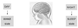
Figure 1: Brain bistability provoked by the solar light cycle.

The internal circadian rhythm is closely synchronized with the cycle of sun light (Fig. 1). Roughly speaking and depending on the particular species, the brain is awake during the day and it is slept during the night, or vice versa. All mammals and birds sleep. There is not a well established law relating the size of the animal with the daily time it spends sleeping, but, in general, large animals tend to sleep less than small animals (Fig. 2). Hence, at first sight, the emergent bistable sleep-wake behavior seems not depend on the precise architecture of the brain nor on its size. This structural property would mean that, if we represent the brain as a complex assembly of units [7, 8, 9], the possible bistability, where large groups of neurons can show some kind of synchronization, should not depend on the topology (structure) nor on the number of nodes (size) of the network (Fig. 3).

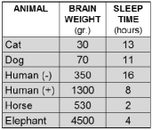
Figure 2: Brain size and mean sleeping time for different animals. (Humans(-) represent new born humans and Humans(+) represent middle age humans).

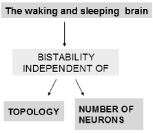
Figure 3: The waking-sleeping brain.

Then, it is essential the type of local dynamics and the excitation/inhibition coupling among the nodes that must be implemented in order to get bistability as a possible dynamical state in a complex network. So, on one side, it has been recently argued [10] that the distribution of functional connections $p(k)$ in the human brain, where $p(k)$ represents the probability of finding an element with $k$ connections to other elements of the network, follows the same distribution of a scale-free network [11], that is a power law behavior, $p(k)\sim k^{-\gamma}$, with $\gamma$ around $2$. This finding means that there are regions in the brain that participate in a large number of tasks while most of the regions are only involved in a tiny fraction of the brain’s activities. On the other side, it has been shown by Kuhn et al. [12] the nonlinear processing of synaptic inputs in cortical neurons. They studied the response of a model neuron with a simultaneous increase of excitation and inhibition. They found that the firing rate of the model neuron first increases, reaches a maximum, and then decreases at higher input rates. Functionally, this means that the firing rate, commonly assumed to be the carrier of information in the brain, is a non-monotonic function of balanced input. These findings do not depend on details of the model and, hence, they are relevant to cells of other cortical areas as well.

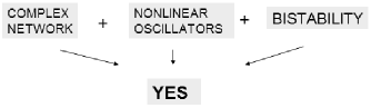
Figure 4: QUESTION: Is it possible to implement some kind of coupling and nonlinear dynamics in each node of a complex network in order to get bistability?. ANSWER: Yes.

Putting together all these facts, we arrive to the central question that we want to bring to the reader: Is it possible to reproduce the bistability in a complex network independently of the topology and of the number of nodes?. The answer is ’Yes’ (Fig. 4). What kind of local dynamics and coupling among nodes must be implemented in order to get this behavior?. In Section 2, we give different possible strategies for the coupling and the local dynamics which should be implemented in a few coupled functional units in order to get a bistable behavior. Then, in Section 3, the same model is exported on a many units network where the desired bistability is also retained. In view of the results, the possibility of constructivism in the world of complex systems in general, and in the neural networks in particular, is suggested in the Conclusion.

2 MODELS OF A FEW COUPLED
FUNCTIONAL UNITS

2.1 General model

Our approach considers the so called functional unit, i.e. a neuron or group of neurons (voxels), as a discrete nonlinear oscillator with two possible states: active (meaning one type of activity) or not (meaning other type of activity). Hence, in this naive vision of the brain as a networked system, if $x_{n}^{i}$, with $0<x_{n}^{i}<1$, represents a measurement of the $ith$ functional unit activity at time $n$, it can be reasonable to take the most elemental local nonlinearity, for instance, a logistic evolution [13], which presents a quadratic term, as a first toy-model for the local neuronal activity:

$$x^{i}_{n+1}=\bar{p}_{i}\;x^{i}_{n}(1-x^{i}_{n}).$$ (1)

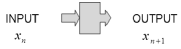
Figure 5: Discrete nonlinear model for the local evolution of a functional unit.

It presents only one stable state for each $\bar{p}_{i}$. Then, there is no bistability in the basic component of our models. For $0<\bar{p}_{i}<1$, the dynamics dissipates to zero, $x_{n}^{i}=0$, then it can represent the functional unit with no activity. For $1<\bar{p}_{i}<4$, the dynamics is non null and it would represent an active functional unit.

We can suppose that this local parameter $\bar{p}_{i}$ is controlled by the signals of neighbor units, simulating in some way the effect of the synapses among neurons. Excitatory and inhibitory synaptic couplings have been shown to be determinant on the synchronization of neuronal firing. For instance, facilitatory connections are important to explain the neural mechanisms that make possible the object representation by synchronization in the visual cortex [14]. While it seems clear that excitatory (symbiotic) coupling can lead to synchronization, frequently inhibition rather than excitation synchronizes firing [15]. The importance of these two kinds of coupling mechanisms has also been studied for other types of neurons, v.g., motor neurons [16].

If a neuron unit simultaneously processes a plurality of binary input signals, we can think that this local information processing is reflected by the parameter $\bar{p}_{i}$. The functional dependence of this local coupling on the neighbor states is essential in order to get a good brain-like behavior (i.e., as far as the bistability of the sleep-wake cycle is concerned) of the network. As a first approach, we can take $\bar{p}_{i}$ as a linear function depending on the actual mean value, $X_{n}^{i}$, of the neighboring signal activity and expanding the interval $(0,4)$ in the form:

$$\bar{p}_{i} = p_{i}\;(3X_{n}^{i}+1),\;\;\;\;\;\;\;(excitation\;\;coupling)$$

$${or}$$

$$\bar{p}_{i} = p_{i}\;(-3X_{n}^{i}+4),\;\;\;\;(inhibition\;\;coupling)$$ (3)

with

$$X_{n}^{i}={1\over N_{i}}\sum_{j=1}^{N_{i}}x_{n}^{j}.$$ (4)

$N_{i}$ is the number of neighbors of the $ith$ functional unit, and $p_{i}$, which gives us an idea of the interaction of the functional unit with its first-neighbor functional units, is the control parameter. This parameter runs in the range $0<p_{i}<p_{max}$, where $p_{max}\geq 1$. When $p_{i}=p$ for all $i$, the dynamical behavior of these networks with the excitation type coupling [7, 8] presents an attractive global null configuration that has been identified as the turned off state of the network. Also they show a completely synchronized non-null stable configuration that represents the turned on state of the network. Moreover, a robust bistability between these two perfect synchronized states is found in that particular model. For different models with a few coupled functional units we sketch in the next subsections the regions where they present a bistable behavior. The details of the complete unfolding [17] of these dynamical systems can be found in the references [18, 19, 20].

2.2 Models of two functional units

Let us start with the simplest case of two interconnected $(x_{n},y_{n})$ functional units. Three different combinations of couplings are possible: $(excitation,excitation)$, $(excitation,inhibition)$ and $(inhibition,inhibition)$.

Figure 6: Two functional coupled units.

As we are concerned with interactions with a certain degree of symbiosis between the coupled units, the regions of parameter space where bistability is found for the first two cases are presented here. Experimental systems where similar couplings have been found or implemented for two cells systems have been reported in the literature [21, 22].

2.2.1 Model with mutual excitation

The dynamics of the $(excitation,excitation)$ case [18] is given by the coupled equations:

$$x_{n+1} = p\;(3y_{n}+1)x_{n}(1-x_{n}),$$ (5)

$$y_{n+1} = p\;(3x_{n}+1)y_{n}(1-y_{n}).$$ (6)

The regions of the parameter space (Fig. 7) where we can find bistability are:

• For $0.75<p<0.86$, the synchronized state, $x_{+}=(\bar{x},\bar{x})=P_{4}$, with $\bar{x}={1\over 3}\{1+(4-{3\over p})^{1\over 2}\}$, which arises from a saddle-node bifurcation for the critical value $p=0.75$, is a stable turned on state. This state coexists with the turned off state $x_{\theta}=0$. The system presents now bistability and depending on the initial conditions, the final state can be $x_{\theta}$ or $x_{+}$. Switching on the system from $x_{\theta}$ requires a level of noise in both functional units sufficient to render the activity on the basin of attraction of $x_{+}$. On the contrary, switching off the two functional units network can be done, for instance, by making zero the activity of one functional unit, or by doing the coupling $p$ lower than $0.75$.

• For $0.86<p<0.95$, the active state of the network is now a period-$2$ oscillation, namely the period-$2$ cycle $(P_{5},P_{6})$ in Fig. 7. This new dynamical state bifurcates from $x_{+}$ for $p=0.86$. A smaller noise is necessary to activate the system from $x_{\theta}$. Making zero the activity of one functional unit continues to be a good strategy to turn off the network.

• For $0.95<p<1$, the active state acquires a new frequency and presents quasiperiodicity (the invariant closed curves of Fig. 7). It is still possible to switch off the network by putting to zero one of the functional units.

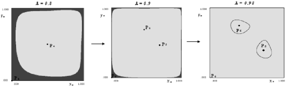
Figure 7: Bistability in $2$ functional units with excitation type coupling ($p=\lambda$).

2.2.2 Model with excitation + inhibition

The dynamics of the $(excitation,inhibition)$ case [19] is given by the coupled equations:

$$x_{n+1} = p\;(3y_{n}+1)x_{n}(1-x_{n}),$$ (7)

$$y_{n+1} = p\;(-3x_{n}+4)y_{n}(1-y_{n}).$$ (8)

The regions of the parameter space (Fig. 8) where we can find bistability are:

• For $1.051<p<1.0851$, a stable period three cycle $(Q_{1},Q_{2},Q_{3})$ appears in the system. It coexists with the fixed point $P_{4}$. When $p$ is increased, a period-doubling cascade takes place and generates successive cycles of higher periods $3\cdot 2^{n}$. The system presents bistability. Depending on the initial conditions, both populations $(x_{n},y_{n})$ oscillate in a periodic orbit or, alternatively, settle down in the fixed point. The borders between the two basins are complex.

• For $1.0851<p<1.0997$, an aperiodic dynamics is possible. The period-doubling cascade has finally given birth to an order three cyclic chaotic band(s) $(A_{31},A_{32},A_{33})$. The system can now present an irregular oscillation besides the stable equilibrium with final fixed populations. The two basins are now fractal.

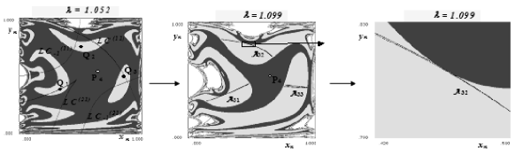
Figure 8: Bistability in $2$ functional units with excitation+inhibition type coupling ($p=\lambda$).

2.3 Models of three functional units

Following the strategy given by relation (2.1-3) several models with three functional units can be established. We have studied in some detail three of them [9, 20] and their bistable behavior is reported here.

2.3.1 Model with local mutual excitation

Let us start with the case of three alternatively interconnected $(x_{n},y_{n},z_{n})$ functional units under a mutual excitation scheme.

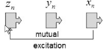
Figure 9: Three alternatively coupled functional units under the excitation scheme.

Then the dynamics of the system is given by the coupled equations:

$$x_{n+1} = p\;(3y_{n}+1)x_{n}(1-x_{n}),$$ (9)

$$y_{n+1} = p\;(3z_{n}+1)y_{n}(1-y_{n}),$$ (10)

$$z_{n+1} = p\;(3x_{n}+1)z_{n}(1-z_{n}).$$ (11)

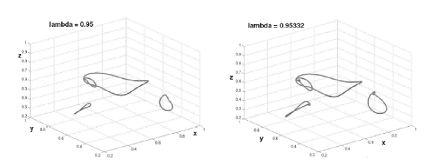
Figure 10: Bistability in $3$ functional units with local excitation type coupling ($p=\lambda$).

The regions of the parameter space where we have found bistability are:

• For $0.93310<p<0.95334$, a big invariant closed curve (ICC) $C1$ coexists with a period-$3$ orbit that bifurcates, first to an order $3$-cyclic ICC (Fig. 10), and finally to an order-$3$ weakly chaotic ring (WCR) before disappearing.

• For $0.98418<p<0.98763$, the ICC $C1$ coexists with another ICC $C2$ (see Ref. [20]) that becomes chaotic, by following a period doubling cascade of tori, before disappearing.

• For $1.00360<p<1.00402$, the ICC $C1$ coexists with a high period orbit that gives rise to an ICC $C3$. This ICC also becomes a chaotic band (see Ref. [20]) by following a period doubling cascade of tori before disappearing.

2.3.2 Model with global mutual excitation

We expose now the case of three globally interconnected $(x_{n},y_{n},z_{n})$ functional units under a mutual excitation scheme.

Then the dynamics of the system is given by the coupled equations:

$$x_{n+1} = p\;(x_{n}+y_{n}+z_{n}+1)x_{n}(1-x_{n}),$$ (12)

$$y_{n+1} = p\;(x_{n}+y_{n}+z_{n}+1)y_{n}(1-y_{n}),$$ (13)

$$z_{n+1} = p\;(x_{n}+y_{n}+z_{n}+1)z_{n}(1-z_{n}).$$ (14)

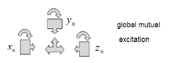
Figure 11: Three globally coupled functional units under the excitation scheme.

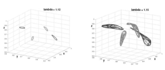
Figure 12: Bistability in $3$ functional units with global excitation type coupling ($p=\lambda$).

For the whole range of the parameter, $0<p<1.17$, bistability is present in this system:

• Firstly, two order-$2$ cyclic ICC coexist before becoming two order-$2$ cyclic chaotic attractors (Fig. 12) by contact bifurcations of heteroclinic type. Finally the two chaotic attractors become a single one before disappearing.

2.3.3 Model with partial mutual excitation

The new case [9] of three partially interconnected $(x_{n},y_{n},z_{n})$ functional units under a mutual excitation scheme is represented in Fig. 13.

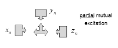
Figure 13: Three partially coupled functional units under the excitation scheme.

The dynamics of the system is given by the coupled equations:

$$x_{n+1} = p\;(3(y_{n}+z_{n})/2+1)x_{n}(1-x_{n}),$$ (15)

$$y_{n+1} = p\;(3(x_{n}+z_{n})/2+1)y_{n}(1-y_{n}),$$ (16)

$$z_{n+1} = p\;(3(x_{n}+y_{n})/2+1)z_{n}(1-z_{n}).$$ (17)

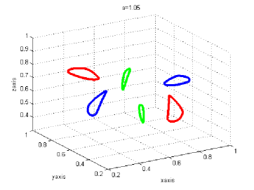
Figure 14: Multistability in $3$ functional units with partial excitation type coupling. The system presents three order-$2$ ICC for $p=a=1.05$.

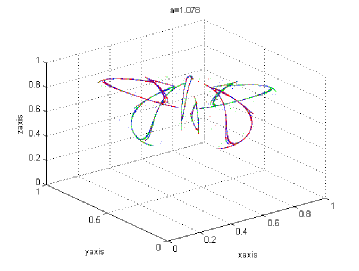
Figure 15: Multistability of three chaotic cyclic attractors of order $2$ for $p=a=1.078$.

The rough inspection of this system puts in evidence the existence of different regions of multistability in the parameter space. These are:

• For $0.93<p<1.04$, there is coexistence among three cycles of period-$2$.

• For $1.04<p<1.06$, the three cycles bifurcate giving rise to three order-$2$ ICC (Fig. 14).

• For $1.06<p<1.08$, the system can present three mode-locked periodic orbits, each one with period multiple of $6$, displaying period doubling cascades giving rise to three chaotic cyclic attractors. Three chaotic cyclic attractors of order $2$ are also possible in this region (Fig. 15).

• For $p>1.08$, the chaotic cyclic attractors collapse in an unique chaotic attractor (Fig. 16).

Also, other multistable situations can be found for some particular values of the parameter $p$ in the former intervals, such as it can be seen in Fig. 17, where the $x$-projection of a generic bifurcation diagram is plotted. Similar diagrams are found for the $y$- and $z$-projections.

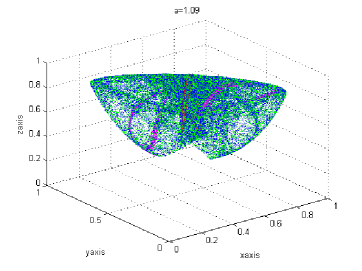
Figure 16: An unique chaotic attractor for $p=a=1.09$.

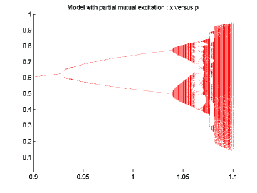
Figure 17: Bifurcation diagram projected in the $x$ coordinate for the initial conditions $(x_{0}=0.37,y_{0}=0.36,z_{0}=0.33)$ as a function of the parameter $p$.

3 MODEL OF MANY COUPLED
FUNCTIONAL UNITS

3.1 The model

The complete synchronization [23, 24] of the network means that $x_{n}^{i}=x_{n}$ for all $i$ , with $i=1,2,\ldots,N$ and $N\gg 1$ [25, 26]. In this regime, we also have $X_{n}^{i}=x_{n}$. The time evolution of the network [8] on the synchronization manifold is then given by the cubic mapping:

$$x_{n+1}=p\;(3x_{n}+1)\;x_{n}(1-x_{n}).$$ (18)

The fixed points of this system are found by solving $x_{n+1}=x_{n}$. The solutions are $x_{\theta}=0$ and $x_{\pm}={1\over 3}\{1\pm(4-{3\over p})^{1\over 2}\}$. The first state $x_{\theta}$ is stable for $0<p<1$ and $x_{\pm}$ take birth after a saddle-node bifurcation for $p=p_{0}=0.75$. The node $x_{+}$ is stable for $0.75<p<1.157$ and the saddle $x_{-}$ is unstable. Therefore bistability between the states

$$x_{n}^{i}=x_{\theta}, \forall i\longrightarrow TURNED\;\;\;OFF\;\;\;STATE,$$ (19)

$$x_{n}^{i}=x_{+}, \forall i\longrightarrow TURNED\;\;\;ON\;\;\;STATE,$$ (20)

seems to be also possible for $p>p_{0}=0.75$ in the case of many interacting units. But stability on the synchronization manifold does not imply the global stability of it. Small transverse perturbations to this manifold can make unstable the synchronized states. Let us suppose then a general local perturbation $\delta x_{n}^{i}$ of the element activity,

$$x_{n}^{i}=x_{*}+\delta x_{n}^{i},$$ (21)

with $x_{*}$ representing a synchronized state, $x_{\theta}$ or $x_{+}$. We define the perturbation of the local mean-field as

$$\delta X_{n}^{i}={3\over N_{i}}\sum_{j=1}^{N_{i}}\delta x_{n}^{j}.$$ (22)

If these expressions are introduced into equation (1), the time evolution of the local perturbations are found:

$$\delta x_{n+1}^{i}=p\,(3x_{*}+1)(1-2x_{*})\delta x_{n}^{i}+p\,x_{*}(1-x_{*})\delta X_{n}^{i}.$$ (23)

The dynamics for the local mean-field perturbation is derived by substituting this last expression in relation (22). We obtain:

$$\delta X_{n+1}^{i}=p\,(3x_{*}+1)(1-2x_{*})\delta X_{n}^{i}+3p\,x_{*}(1-x_{*}){1\over N_{i}}\sum_{j=1}^{N_{i}}\delta X_{n}^{j}.$$ (24)

We express now the local mean-field perturbations of the first-neighbors as function of the local mean-field perturbation $\delta X_{n}^{i}$ by defining the local operational quantity $\sigma_{i}^{n}$,

$${1\over N_{i}}\sum_{j=1}^{N_{i}}\delta X_{n}^{j}=\sigma_{n}^{i}\;\delta X_{n}^{i},$$ (25)

which is determined by the dynamics itself. If we put together the equations (23-24), the linear stability of the synchronized states holds as follows:

$$\left(\begin{array}[]{c}\delta x_{n+1}^{i}\\ \delta X_{n+1}^{i}\end{array}\right)=\left(\begin{array}[]{cc}p\,(3x_{*}+1)(1-2x_{*})&p\,x_{*}(1-x_{*})\\ 0&p\,(3x_{*}+1)(1-2x_{*})+3p\,\sigma_{n}^{i}\,x_{*}(1-x_{*})\end{array}\right)\left(\begin{array}[]{c}\delta x_{n}^{i}\\ \delta X_{n}^{i}\end{array}\right).$$ (26)

Let us observe that the only dependency on the network topology is included in the quantity $\sigma_{n}^{i}$. The rest of the stability matrix is the same for all the nodes and therefore it is independent of the local and global network organization.

The turned off state is $x_{*}=x_{\theta}=0$. The eigenvalues of the stability matrix are in this case $\lambda_{1}=\lambda_{2}=p$. Then, this state is an attractive state in the interval $0<p<1$. It loses stability for $p=1$, then the highest value $p_{f}$ of the parameter $p$ where bistability is still possible satisfies $p_{f}\leq 1$.

The turned on state $x_{+}$ verifies $x_{*}=x_{+}={1\over 3}\{1+(4-{3\over p})^{1\over 2}\}$. If we suppose $\sigma_{n}^{i}=\sigma$, the eigenvalues of the stability matrix are $\lambda_{1}=2-2p-p(4-{3\over p})^{1\over 2}$ and $\lambda_{2}=\lambda_{1}+{\sigma\over 3}(3-2p+p(4-{3\over p})^{1\over 2})$. Let us observe that $\lambda_{1}=-1$ for $p=1$. This implies that the parameter $p_{c}$ for which the synchronized state $x_{+}$ looses stability verifies $p_{c}\leq 1$. Depending on the sign of $\sigma$, we can distinguish two cases in the behavior of $p_{c}$:

• If $0<\sigma<1$, we find that $\mid\lambda_{2}\mid<1$. Then $x_{+}$ bifurcates through a global flip bifurcation for $p=p_{c}=1$. In this case, the bifurcation of the synchronized state $x_{+}$ for $p_{c}=1$ coincides with the loss of the network bistability for $p_{f}=1$. Hence $p_{c}=p_{f}=1$ for this kind of networks, and the bistability holds between $x_{\theta}$ and $x_{+}$ in the parameter interval $p_{0}=0.75<p<p_{c}=p_{f}=1$. As an example, an all-to-all network shows this behavior because $\sigma=1$. This is represented in the inset of Fig. 18.

• If $-1<\sigma<0$, then $\lambda_{2}=-1$ is obtained for a $p=p_{c}$ smaller than $1$. Therefore it is now possible to obtain an active state different from $x_{+}$ in the interval $p_{c}<p<p_{f}$. For instance, simulations show that the global flip bifurcation of the synchronized state for a scale free network occurs for $p_{c}=0.87\pm 0.01$. A value of $p=0.866$ is obtained from the stability matrix by taking $\sigma=-1$. For this particular network it is also found that $p_{f}=1$. Then, bistability is possible in the range $p_{0}=0.75<p<p_{f}=1$ for this kind of configuration. But now an active state with different dynamical regimes is observed in the interval $p_{c}=0.87<p<p_{f}=1$. If we identify the capacity of information storing with the possibility of the system to access to complex dynamical states, then, we could assert, in this sense, that a scale free network has the possibility of storing more elaborated information in the bistable region that an all-to-all network.

Figure 18: Stable states $(x_{\theta},x_{+})$ of the network for $0<p<1$. Let us observe the two zones of bistability: $p_{0}<p<p_{c}$ and $p_{c}<p<p_{f}$. The main figure corresponds to a scale free network made up of $N=10^{4}$ elements: $p_{0}=0.75$, $p_{c}=0.87\pm 0.01$ and $p_{f}=1$. The inset shows the same graph but in an all-to-all network of the same size: $p_{0}=0.75$, $p_{c}=p_{f}=1$. Initial conditions for the $x_{i}$’s were drawn from a uniform probability distribution in the interval $(0,1)$.

Let us note that $\sigma$ also indicates a different behavior of local dissipation, as expression (25) suggests. A positive $\sigma$ means a local in-phase oscillation of the node signal and mean-field perturbations. A negative $\sigma$ is meaning a local out of phase oscillation between those signal perturbations. Hence, $\sigma$ also brings some kind of structural network information. In all the cases the stability loss of the completely synchronized state is mediated by a global flip bifurcation. The new dynamical state arising from that active state for $p=p_{c}$ is a periodic pattern with a local period-$2$ oscillation. The increasing of the coupling parameter monitors other global bifurcations that can lead the system towards a pattern of local chaotic oscillations.

3.2 Transition between On-Off States

We proceed now to show the different strategies for switching on and off a random scale free network. The choice of this network is suggested by the recent work [10] on the connections distribution among functional units in the brain. They find it to be a power-law distribution. Following this insight [8], a scale-free network following the Barabási-Albert (BA) recipe [11] is generated. In this model, starting from a set of $m_{0}$ nodes, one preferentially attaches each time step a newly introduced node to $m$ older nodes. The procedure is repeated $N-m_{0}$ times and a network of size $N$ with a power law degree distribution $P(k)\sim k^{-\gamma}$ with $\gamma=3$ and average connectivity $\langle k\rangle=2m$ builds up. This network is a clear example of a highly heterogenous network, in that the degree distribution has unbounded fluctuations when $N\rightarrow\infty$. The exponent reported for the brain functional network has $\gamma<3$. However, studies of percolation and epidemic spreading [27, 28] on top of scale-free networks have shown that the results obtained for $\gamma=3$ are consistent with those corresponding to lower values of $\gamma$, with $\gamma>2$. As explained before, network bistability between the active and non active states is here possible in the interval $p_{0}=0.75<p<p_{f}=1$ (Fig. 18).

Switching off the network

Two different strategies [8] can be followed to carry the network from the active state to that with no activity (Fig. 18).

• Route I: By doing the coupling $p$ lower than $p_{0}$. This is the easiest and more natural way of performing such an operation. In our naive picture of a brain-like system, it could represent the decrease (or increase, it depends on the specific function) of the synaptic substances that provokes the transition from the awake to the sleep state. The flux of these chemical activators is controlled by the internal circadian clock, which is present in all animals, and which seems to be the result of living during millions of years under the day/night cycle.

• Route II: By switching off a critical fraction of functional units for a fixed $p$. Evidently, at first sight, this strategy has no relation with the behavior of a real brain-like system. Thus, this is done by looking over all the elements of the network, and considering that the element activity is set to zero with probability $\lambda$ (which implies that on average $\lambda N$ elements are reset to zero). The result of this operation is shown in Fig. 19. Here, it is plotted for different $p$’s the relative size of the biggest (giant) cluster of connected active nodes in the network versus $\lambda$. Note that this procedure does not take into account the existence of connectivity classes, but all nodes are equally treated. The procedure is thus equivalent to simulations of random failure in percolation studies [27]. The strategy in which highly connected functional units are first put to zero is more aggressive and leads to quite different results.

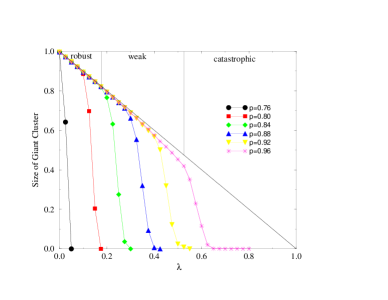
Figure 19: Turning off a scale free network. Three different phases in the behavior of the giant cluster size versus $\lambda$ (fraction of switched off nodes) are observed. These three phases are illustrated for $p=0.96$: the robust phase, the weak phase and the catastrophic phase (see the text). Other network parameters are as those of Fig. 18.

Each curve presents three different zones depending on $\lambda$:

- the robust phase: For small $\lambda$, the network is stable and only those states put to zero have no activity. There is a linear dependence on the giant cluster size with $\lambda$. In this stage, the switched off nodes do not have the capacity to transmit its actual state to its active neighbors.

- the weak phase: For an intermediate $\lambda$, the nodes with null activity can influence its neighborhood and switch off some of them. The linearity between the size of the giant cluster and $\lambda$ shows a higher absolute value of the slope than in the robust zone.

- the catastrophic phase: When a critical $\lambda_{c}$ is reached, the system undergoes a crisis. The sudden drop in this zone means that a small increase of the non active nodes leads the system to a catastrophe; that is, the null activity is propagated through all the network and it becomes completely down.

It is worth noticing that when the system is outside the bistability region for $p>1$, the catastrophic phase does not take place. Instead, the turned off nodes do not spread its dynamical state and the neighboring nodes do not die out. This is because the dynamics of an isolated node is self-sustained when $p>1$. Consequently, it is observed that the network breaks down in many small clusters and the transition resembles that of percolation in scale free nets [27, 29].

Switching on the network

Two equivalent strategies [8] can be followed for the case of turning on the network (Fig. 20):

• (I) For a fixed $p$, we can increase the maximum value $\epsilon$ of the noisy signal, which is randomly distributed in the interval $(0,\epsilon)$ over the whole system. When $\epsilon$ attains a critical value $\epsilon_{c}$, the noisy configuration can leave the basin of attraction of $x_{\theta}$, whose boundary seems to have the form in phase space of a “hollow cane” around it, and then the network rapidly evolves toward the turned on state;

• (II) If this operation is executed by letting $\epsilon$ to be fixed and by increasing the coupling parameter $p$, the final result of switching on the network is reached when $p$ takes the value for which $\epsilon=\epsilon_{c}$. The final result is identical in both cases.

Let us remark that the strategy equivalent to the former Route II, that is, the switching on of a critical fraction of functional units, is not possible in this case. It is a consequence of the fact that a switched off functional unit can not be excited by its neighbors and it will maintain indefinitely the same dynamical state ($x_{i}=0$).

Finally, let us note that, from Fig. 20, a bigger $p$ requires a smaller $\epsilon_{c}$ to switch on the net. Observe that this behavior could be interpreted in our approach as the smaller level of noise that is needed for awaking a brain-like system that it is departing from the sleeping state.

Figure 20: Turning on a scale free network. For a fixed $p$, a noisy signal randomly distributed in the interval $(0,\epsilon)$ is assigned to every node. When $\epsilon$ reaches the critical level $\epsilon_{c}$ the network becomes switched on. Other network parameters are as those of Fig. 18.

4 CONCLUSION

One of the more challenging problems in nonlinear science is the goal of understanding the properties of neuronal circuits [30]. Synchrony and multistability are two important dynamical behaviors found in those circuits [31, 32, 33]. In this work, different coupling schemes for networks with local logistic dynamics are proposed [7]. It is observed that these types of couplings generate a global bistability between two different dynamical states [8, 9]. This property seems to be topology and size independent. This is a direct consequence of the local mean-field multiplicative coupling among the first-neighbors. If a formal and naive relationship is established between these two states and the sleep-wake states of a brain, respectively, one would be tempted to assert that these types of couplings in a network, regardless of its simplicity, give us a good qualitative model for explaining that specific bistability. Following this insight, several low-dimensional systems with logistic components coupled under these schemes have been presented and the regions where the dynamics shows bistability have been identified. The extension of this type of coupling to a general network with local logistic dynamics has also been achieved. This system presents global bistability between an active synchronized state and another synchronized state with no activity. This property is topology and size independent. This is a direct consequence of the local mean-field multiplicative coupling among the first-neighbors. If a formal and naive relationship is established between the switched off and switched on states of that network, and the sleep-wake states of a brain, respectively, one would be tempted to assert that this model, regardless of its simplicity, is a good qualitative representation for explaining that specific bistability. Furthermore, on more theoretical grounds, the results obtained here point out the entangled interplay between topology and function in networked systems [34] where complex structures coexist with nonlinear dynamics.

References

- [1] Cajal, S.R. The structure and connections of neurons; Nobel Lecture; December 12, Stockholm, 1906.
- [2] Llinás, R.R. Nat. Rev. Neurosci. 2003, vol. 4, 77-80.
- [3] Carey J.(Editor) Brain Facts; Fifth revised edition, Publications of the Society for Neuroscience; Washington, 2006.
- [4] Abarbanel H.D.I.; Gibb L.; Mindlin G.B.; Talathi S. J. Neurophysiol. 2004, vol. 92, pp. 96-110.
- [5] Winfree A.T. The timing of biological clocks; Scientific American Library; New York, 1986.
- [6] Bar-Yam Y. Dynamics of Complex Systems; Westview Press; New York, 1997.
- [7] Lopez-Ruiz R.; Fournier-Prunaret D. MEDYFINOL’06 Conference, AIP Proceedings 2007, vol. 913, 89-95.
- [8] Lopez-Ruiz R.; Moreno Y.; Pacheco, A.F.; Boccaletti, S.; Hwang, D.-U. Neural Networks 2007, vol. 20, 102-108.
- [9] Lopez-Ruiz R.; Fournier-Prunaret, D. NOMA’09 Conference, Proceedings 2009, 6-9.
- [10] Eguiluz V.M.; Chialvo, D.R.; Cecchi, G.; Baliki, M.; Apkarian, A.V. Phys. Rev. Lett. 2005, vol. 94, 018102(4).
- [11] Barabási A.L.; Albert R. Science 1999, vol. 286, 509-512.
- [12] Kuhn A.; Aertsen, Ad.; Rotter, S. J. Neurosci. 2004, vol. 24, 2345-2356.
- [13] May R.M. Nature 1976, vol. 261, 459-467.
- [14] Eckhorn, R.; Gail, A.M.; Bruns, A.; Gabriel, A.; Al-Shaikhli, B.; Saam, M. IEEE Trans. Neural Netw. 2004, vol. 15, 1039-1052.
- [15] Vreeswijk1 C.V.; Abbott, L.F.; Ermentrout, G.B. J. Comput. Neurosci. 1994, vol. 1, 313-321.
- [16] Koenig, J.H.; Ikeda, K. J. Comp. Physiol. A. 1983, vol. 150, 305-317.
- [17] Mira C.; Gardini, L.; Barugola, A.; Cathala, J.-C. Chaotic Dynamics in Two-Dimensional Noninvertible Maps; series A, vol. 20; World Scientific Publishing; Singapore, 1996.
- [18] Lopez-Ruiz, R.; Fournier-Prunaret, D. Math. Biosci. Eng. 2004, vol. 1, 307-324.
- [19] Lopez-Ruiz, R.; Fournier-Prunaret, D. Chaos, Solitons and Fractals 2005, vol. 24, 85-101.
- [20] Fournier-Prunaret, D.; Lopez-Ruiz, R.; Taha, A.K. Grazer Mathematische Berichte 2006; vol. 350, 82-95.
- [21] Graham, D.W.; Knapp, C.W.; Van Vleck, E.S.; Bloor, K.; Lane, T.B.; Graham, C.E. ISME Journal 2007, vol. 1, 385-393.
- [22] Mihailovic, D.T.; Balaz, I. Mod. Phys. Lett. B 2012, vol. 26, 1150031(9).
- [23] Lopez-Ruiz, R.; Perez-García, C. Chaos, Solitons and Fractals 1991; vol. 1, 511-528.
- [24] Boccaletti, S.; Kurths, J.; Osipov, G.; Valladares, D.L.; Zhou, C.S. Phys. Rep. 2002; vol. 366, 1-101.
- [25] Jalan, S.; Amritkar, R.E. Phys. Rev. Lett. 2003; vol. 90, 014101(4).
- [26] Oprisan S.A. Int. J. Neurosci. 2009; vol. 119, 482-491.
- [27] Callaway, D.S.; Newman, M.E.J.; Strogatz, S.H.; Watts, D.J. Phys. Rev. Lett. 2000; vol. 85, 5468-5471.
- [28] Dorogovtsev, S.N.; Mendes, J.F.F. Evolution of Networks. From Biological Nets to the Internet and the WWW; Oxford University Press; Oxford, 2003
- [29] Vázquez, A.; Moreno, Y. Phys. Rev. E 2003, vol. 67, 015101(R).
- [30] Rabinovich, M.I.; Varona, P.; Selverston, A.I.; Abarbanel, H.D.I. Rev. Mod. Phys. 2006, vol. 78, 1213-1265.
- [31] Borgers, C.; Kopell, N. Neural Comput. 2003, vol. 15, 509-538.
- [32] Hansel, D.; Mato, G. Neural Comput. 2003; vol. 15, 1-56.
- [33] Buzsàki, G.; Geisler, C.; Henze, D.A.; Wang, X.-J. Trends in Neurosciences 2004, vol. 27, 186-193.
- [34] Strogatz, S.H. Nature (London) 2001; vol. 410, 268-276.