Uniform Shock Waves in Disordered Granular Matter

Abstract

The confining pressure $P$ is perhaps the most important parameter controlling the properties of granular matter. Strongly compressed granular media are, in many respects, simple solids in which elastic perturbations travel as ordinary phonons. However, the speed of sound in granular aggregates continuously decreases as the confining pressure decreases, completely vanishing at the jamming-unjamming transition. This anomalous behavior suggests that the transport of energy at low pressures should not be dominated by phonons. In this work we use simulations and theory to show how the response of granular systems becomes increasingly nonlinear as pressure decreases. In the low pressure regime the elastic energy is found to be mainly transported through nonlinear waves and shocks. We numerically characterize the propagation speed, shape, and stability of these shocks, and model the dependence of the shock speed on pressure and impact intensity by a simple analytical approach.

I Introduction

Granular systems are materials formed by conglomerates of macroscopic particles repelling through their mutual contact Metha . These, a priori, simple systems exhibit complex collective behavior and physical response. For example, depending on external conditions, granular media are found in fluid or solid phases, with defined characteristic features JaegerRMP . Despite the visual analogy with more conventional matter, the nature of these granular phases is far from being well understood.

Key to better understanding the behavior and response of granular systems is the study of the mechanisms of energy transport and dissipation. Experiments on elastic wave propagation have shown that the confining pressure $P$ controls the speed of sound $c$ of the medium Jiaprl1999 -Jiaprl2004 , causing it to scale all the way to zero at low pressure. Several works have shown that for high confining pressures the speed of sound scales as $c\sim P^{1/6}$, a relation that can be rationalized from an effective medium theory. However, at low confining pressures a much faster power law is observed $c\sim P^{1/4}$, whose physical origin still remains unclear. In general, the complexity of wave propagation in granular matter is evidenced by the coda-like signal spectrum of elastic waves, originated from the scattering of sound with the heterogeneities of the media Jiaprl1999 ,Jiaprl2004 .

From the theoretical point of view, much of the current understanding of granular mechanics comes from a simple microscopic approach, where granular media are modeled as amorphous packings of soft repulsive spheres Durian -MvHecke . Using this simple model, the elastic response has been mainly studied in the linear regime, by applying a conventional normal mode expansion of the potential energy Feng -Tighe . Following this normal mode approximation, different studies revealed that strongly compressed granular media have a vibrational spectrum which follows the Debye law, and therefore, their elastic behavior parallels the one of simple atomic solids.

Such studies also revealed an anomalous behavior in the elastic response as the pressure on the medium decreases, and the system approaches the jamming/unjamming transition. In this low pressure regime it was found that the vibrational modes resemble ordinary phonons only below a characteristic frequency $\omega^{*}$, that vanishes as $P$ goes to zero LSilbert ; Wyart . Above $\omega^{*}$ the modes are still extended but strongly scattered by disorder, hence their ability to transport energy is impaired Xu ; Vitelli . This suggests that granular media behave like a continuum elastic medium only above a characteristic length scale $l^{*}$ (thought to be related with $\omega^{*}$) which diverges as $P$ goes to zero Wyart .

However, there is still another source of anomalous behavior in the low pressure regime, which is universally displayed by granular media, but it has received far less attention. As a direct consequence of the nonlinear dependence of the local contact force on the grain deformations, the sound speed of a granular medium vanishes as $P$ goes to zero Nesterenko1984 , NesterenkoBook . This fact suggests that the transport of energy in the low pressure regime should not be dominated by phonons. Actually, linear sound does not even exist at the jamming point, and a phononic description here looses its validity. Thus, we can expect that at low pressures the transport of energy in granular media would be dominated by supersonic non-linear waves and shocks.

This peculiar property of a vanishing sound speed at non-vanishing densities, not found in other systems like gases, liquids or solids, was first studied by V. Nesterenko, who conceived the name sonic vacuum for a media whose sound speed is exactly zero Nesterenko1984 , NesterenkoBook . Nesterenko and coworkers mainly analyzed the consequences of the sonic vacuum in the transport of energy in ordered granular chains Nesterenko1984 -Sen . In such cases elastic energy was found to be transported in the form of non-linear solitary waves (characteristic energy pulses that propagate without shape distortion).

Despite the results for ordered chains, the mechanisms of non-linear energy transport in disordered granular matter is largely unexplored Sinkovits ; Gomez . In particular, it is not clear what role the structural disorder of the medium plays. Moreover, no systematic study exist of the expected crossover between the linear waves obtained at strong confining pressures and the nonlinear waves expected to dominate in the low pressure regime, when the granular medium is close to the jamming/unjamming transition.

In this work, we study the non-linear transport of energy in $2D$ disordered granular matter by using numerical simulations and theoretical calculations. Here we focus on the full response of two-dimensional granular packings when they are dynamically compressed by an external piston. These experiments cause the formation of steadily propagating fronts, without attenuation, nor deceleration, allowing the clear determination of the nature of the associated elastic waves (which can be linear, weakly non-linear, or strongly non-linear). By using this approach, we show how the elementary excitations of systems at low pressures are shocks waves rather than ordinary linear phonons Gomez . We provide a full characterization of these shocks, studying features like shape, propagation speed, and stability. We also present a simple model which accurately describes the propagation of the shocks, and the crossover from shocks to linear waves, as the pressure increases, or the driving strength decreases.

The paper is organized as follow: In section II, we describe the numerical model and the molecular dynamics simulations. In section III, we present the numerical results related to the formation of shock waves by piston compression experiments. In section IV, we develop an analytical model which captures the speed of the shocks from the nearly linear to the strongly nonlinear regime using conservation laws. The appendices present an alternative approach to this behavior: a continuum equation of motion (a simplification of Nesterenko’s) is derived in Appendix A while its soliton and shock solutions are presented in Appendix B.

II Numerical model and simulations

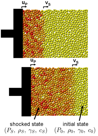
Figure 1: Piston compression experiments. A continuous compression of the system by a piston moving at velocity $u_{P}$ leads to the formation of a pressure front (shock wave) travelling at a velocity $v_{S}$. The shock compression process can be seen as a fast transition between two states (initial and shocked) of the granular system.

Materials with granularity, as diverse as sand, rocks, ceramics, foams, or emulsion, can exhibit a universal elastic response which is well described by a simple microscopic approach Durian -MvHecke . In all these systems the elasticity is governed by the soft contact interaction between the grains. In the simplest model of frictionless spherical grains, the contact potential between two grains $i$ and $j$, located at positions $\vec{x}_{i}$ and $\vec{x}_{j}$, is written as Somfai :

$$\begin{cases}U_{ij}=\frac{\varepsilon_{ij}}{\alpha}\,\,\delta_{ij}\,^{\alpha}\,\,\,\,\,\,\,\,if\,\,\,\,\,\delta_{ij}>0\\ U_{ij}=0\,\,\,\,\,\,\,\,\,\,\,\,\,\,\,\,\,\,\,\,\,\,\,\,\,\,if\,\,\,\,\,\delta_{ij}\leq 0\end{cases}$$ (1)

where the overlap between particles is given by $\delta_{ij}\equiv R_{i}+R_{j}-|\vec{x}_{i}-\vec{x}_{j}|$, where ${R_{i}}$ is the radius of the $i^{th}$ particle. The exponent $\alpha$ gives the strength of the interaction. The case $\alpha=5/2$ corresponds to the widely used Hertz’s law. The interaction parameter $\varepsilon_{ij}=\frac{4}{3}\frac{R_{i}R_{j}}{R_{i}+R_{j}}E^{*}_{ij}$ is expressed in terms of the effective Young’s modulus of the two particles, $E^{*}_{ij}$; see Ref. Somfai for more details.

We model granular media by means of jammed amorphous packings of particles interacting through the Hertzian law ($\alpha=5/2$). The packings are prepared at a fixed pressure $P$, or equivalently, an average particle overlap $\delta_{0}\sim P^{2/3}$, by using a molecular dynamics algorithm Somfai . Similar structures are also commonly obtained through conjugate gradient algorithms. In order to avoid crystallization, the particle radii are uniformly distributed between 0.8 and 1.2 times their average radius. Typical packings are in the range of $10^{3}$ to $10^{4}$ grains with various width to length ratios.

In this work, we study the transport of energy by means of piston compression experiments. Here an initially jammed configuration is continuously compressed by a piston which moves with a constant velocity $u_{P}$ in the $X$ direction, see the schematic in Fig.  1. The subsequent motion of the particles is obtained by numerical integration of Newton’s equations of motion using the Verlet algorithm Allen . We employ periodic boundary conditions in the $Y$ direction and a fixed boundary on the right edge of the system. In our simulations, the unit of mass is set by fixing the grain density to unity. The effective particle Young modulus $E^{*}$ is set to one, which becomes the pressure unit. These choices ensure that the speed of sound inside the grain, $v_{g}$ is one Somfai . Lengths are measured in units of average particle diameter.

Piston compression experiments have been previously used in studies of shock waves travelling through different media, like gases, liquids, or crystals Courant -MeyersBook . In all these systems a travelling pressure front is observed as a consequence of the motion of the piston. In general, the velocity and shape of the front reveals important information about the mechanisms of energy transport.

III Numerical Results

III.1 Phenomenology of Shocks

Simulations at different compression velocities show that piston compression experiments induce the formation of travelling pressure fronts (Fig.  1). Ahead of the front there is an undistorted static region where the particles remain at rest having their initial overlap $\delta_{0}$. This initial state is characterized by the original values of pressure $P_{0}$, density $\rho_{0}$, strain $\gamma_{0}$, and speed of sound $c_{0}$. Behind the front we find a compressed region where the particles have acquired some kinetic energy.

During their propagation the fronts remain essentially flat, such that to a good approximation the compression experiments can be described as one dimensional processes. We present a detailed analysis and discussion of front stability and roughness at the end of the numerical results.

Taking advantage of the flatness of the front, we average over the transverse direction $y$, and obtain profiles of the averaged pressure $P(x)$, density $\rho(x)$, and the $x$ component of the particle velocity $u(x)$, as a function of the coordinate $x$. Figures 2a and 2b show the advance of a typical front, as seen through averaged profiles of pressure and velocity. Note that the velocity profiles show that behind the shock front the particles move on average at the piston velocity $u_{P}$.

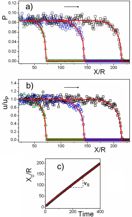
Figure 2: Phenomelology of shock waves. Propagation of fronts as seen through the profiles of the averaged pressure $P$ (a), and averaged particle velocity $u$ normalized with the piston velocity $u_{P}$ (b). The front moves in the direction of the arrows. Different curves corresponds to profiles at different times and the red lines are phenomenological fits. c) Position of the front as a function of time. Note that at long times the front moves linearly with time (red line), with a propagation speed $v_{S}$.

In the steady state regime, the compression front attains a stationary shape described by an empirical fit, drawn as continuous lines in Fig. 2a and 2b. In general, the speed of propagation and the shape of the profiles depend on (1) the degree of non-linearity of the shocks and (2) the compression velocity $u_{P}$. In the next sections, we present a full characterization of such dependencies. By tracking the position of the profiles we find that after transients have died out, the front travels linearly in time $t$, propagating thus with a characteristic constant speed $v_{S}$, see Fig. 3. The determination of the propagation velocity allows the identification of the compression fronts with non-linear supersonic shock waves ($v_{S}\gg c_{0}$), or linear waves ($v_{S}=c_{0}$).

From the averaged profiles it is clear that the particles behind the front remain in a rather homogeneous state (see Fig. 2a and 2b). This region is well characterized by the average values $P_{S}$, $\rho_{S}$, $\gamma_{S}$ and $c_{S}$. Thus, the passage of the front can be seen as a transition in the granular media from an initial ($P_{0}$, $\rho_{0}$, $\gamma_{0}$, $c_{0}$) to a compressed state ($P_{S}$, $\rho_{S}$, $\gamma_{S}$, $c_{S}$). This behavior is strikingly different from the profiles observed in crystals or crystalline arrays of grains, where large oscillations in pressure, density, or particle velocity are observed behind the fronts NesterenkoBook ,HolianToda ,BringaNuclear .

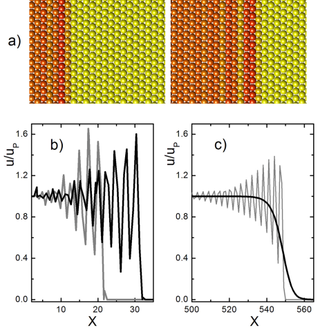
Figure 3: Shock waves in a granular crystal. a) Cartoons of the pressure oscillations as a consequence of the in-phase motion of crystalline planes (red colors indicate regions of higher pressure). b) Propagation of the shock wave as seen through the particle velocity profiles. The front travels from left to right. c) Shock profiles in the presence of viscosity, for viscosity coefficients above (thick black line) and below (thin grey line) critical value.

As an example, Fig. 3a shows the propagation of a shock wave obtained though the uniform compression of a granular crystal of hexagonal symmetry with zero pre-compression ($\delta_{0}=0$). Figure 3b shows the propagation of the shock as seen through the particle velocity profiles. Here the large coherent oscillations are caused by the in-phase motion of the crystalline planes. Note also that these oscillations change with time (compare grey and black curves corresponding to the time evolution), such that the profile never reaches a steady state.

We believe that the underlying mechanism of equilibration producing the homogenization of the profiles in the amorphous systems is intrinsically related with the structural disorder. In our amorphous structures the disorder prevents any coherent oscillation, such that the peaks are washed out, leaving an homogeneous state. Similar homogenous states are also commonly observed in the compression of other unstructured systems, like gases or liquids Courant -MeyersBook .

In ordered systems, homogeneous shock profiles are obtained when some source of dissipation is present Duvall ,Herbold . Figure 3c shows a steady shock wave profile (black line) obtained when a viscous dissipation term, based on the relative velocities between particles, is added to the force: $f_{i,j}=\eta|v_{i}-v_{j}|$, where $\eta$ is the viscous coefficient. In this figure the viscosity coefficient has been chosen high enough to obtain a steadily propagating profile without oscillations. For values of the viscosity coefficient smaller than a critical value, the obtained fronts reach steady profiles that still display some residual oscillations (Fig. 3c, gray line). These conclusions, concerning the effect of viscosity on the shock profile, are demonstrated mathematically in Appendix B.

Although our disordered granular structures do not have any source of real dissipation, the obtained uniform shock profiles suggest that the disorder of the system could be playing the role of an effective viscosity Gomez .

III.2 Jump Conditions

Mathematically, the propagation of fronts can be studied through the conservation of mass, momentum, and energy:

$$\begin{cases}\rho_{t}+(\rho\,u)_{x}=0\\ (\rho\,u)_{t}+(\rho\,u^{2}+P)_{x}=0\\ (\frac{1}{2}\rho u^{2}+U)_{t}+[u(\frac{1}{2}\rho u^{2}+U+P)]_{x}=0\end{cases}$$ (2)

In the case of the propagation of uniform shocks, as found in our simulations (Fig. 2), the (approximate) uniformity of $\rho$, $P$ and $u$ ahead and behind the shock front allows the immediate integration of the equations, leading to a set of relationships known as the Rankine-Hugoniot jump conditions Courant -MeyersBook :

$$\begin{cases}\rho_{0}v_{S}=\rho_{S}(v_{S}-u_{P})\\ \rho_{0}\,v_{S}^{2}+P_{0}=\rho_{S}\,(u_{P}-v_{S})^{2}+P_{S}\\ \frac{1}{2}\rho_{0}v_{S}^{3}+v_{S}\,U_{0}+v_{S}\,P_{0}=\\ \frac{1}{2}\rho_{S}(v_{S}-u_{P})^{3}+(v_{S}-u_{P})\,U_{S}+(v_{S}-u_{P})\,P_{S}\end{cases}$$ (3)

Here the results are expressed in the reference frame of the shock front. In this frame, the shock is in a steady state and the net flow of mass, momentum, and energy toward the shock has to be zero. The quantities $\rho_{0},\rho_{S},P_{0},P_{S},$ and $U_{0},U_{S}$ are respectively the density, pressure, and internal energy density before and after the passage of the shock.

In the case of a 1d chain, the density takes the simple form $\rho=\frac{M}{2R-\delta}$ and the conservation of mass leads to a relation between the characteristic velocities $u_{P}$ and $v_{S}$, through the average radius of the particles, $R$, and the compressions in and ahead of the shock, $\delta_{S}$ and $\delta_{0}$ respectively:

$$v_{S}=u_{P}\,\frac{2R-\delta_{0}}{\delta_{S}-\delta_{0}}~{}.$$ (4)

Note that since the particle compression $\delta_{S}$ is typically much smaller than its diameter $2R$, Eq. (4) implies that $v_{S}\gg u_{P}$. In the limiting case of hard incompressible spheres $v_{S}\longrightarrow\infty$. In reality, there is an upper cut-off to the speed $v_{s}$ given by the sound speed within the grain, that is equal in the case of steel to approximately 6000 m/s .

III.3 Shock’s speed

Commonly, the nature of the traveling fronts (linear or non-linear) depends on both piston velocity $u_{P}$ and initial pressure applied on the system $P_{0}$. Here, we analyze changes in the features of wave propagation by tracking variations in the front speed as a function of piston velocity and the initial confining pressure $P_{0}$, which measures the distance of the uncompressed system to the unjamming transition, which occurs when $P_{0}\rightarrow 0$. This allows us to determine when nonlinear sound propagation takes over from the linear propagation.

Figure 4a shows the results of this study. Note that for any finite initial pressure $P_{0}$, at low compression velocities $u_{P}$ the fronts travel with velocities $v_{S}$ which are roughly independent of $u_{P}$. This is evidence of a regime of linear/weakly nonlinear wave propagation. Here the fronts travel at approximately the longitudinal speed of sound of the media $v_{S}\sim c_{0}$. In this regime, the propagation speed is simply controlled by the initial confining pressure $P_{0}$ or initial overlap $\delta_{0}$.

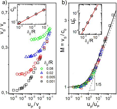
Figure 4: Propagation speed. a) Speed of the front $v_{S}$ versus particle velocity $u_{P}$ measured in units of $v_{g}$, the sound speed within the grain, for decreasing particle overlap $\delta_{0}$. The inset shows the variation of the sound speed $c_{0}$ with the initial overlap $\delta_{0}$ (data) and the scaling $c_{0}\sim delta_{0}^{1/4}$ (line). b) Normalized plot obtained be rescaling $v_{S}$ with $c_{0}$ $v_{S}(0)$ and $u_{P}$ with $u_{P}^{\star}$. The dashed line indicates the power law $v_{S}\sim{u_{P}}^{1/5}$ characteristic of a sonic vacuum. The inset shows the variation of $u_{P}^{\star}$ with the initial overlap $\delta_{0}$ (data) and the scaling $u_{P}^{\star}\sim\delta_{0}^{5/4}$ (line).

The inset of Fig. 4a shows the obtained variation of the speed of sound $c_{0}$ with the initial overlap $\delta_{0}$. The functional variation of $c_{0}$ with $\delta_{0}$ can be rationalized using scaling arguments. Note that in general $c_{0}\sim\sqrt{B}$, where the bulk modulus $B=\frac{\partial P}{\partial V}$ and $P=\frac{\partial E}{\partial V}$. The change in volume $dV$ scales linearly with $\delta_{0}$, the average overlap between particles, while the energy scales as $E\sim\delta_{0}^{\alpha}$, see Eq. 1. Upon setting $\alpha=5/2$, we obtain the pressure dependence of the longitudinal speed of sound $c_{0}\sim\delta^{1/4}_{0}\sim P^{1/6}$ valid for Hertzian interactions Somfai . The inset of Fig. 4a shows that the numerical data for $c_{0}$, represented by symbols, is consistent with the $\delta_{0}^{1/4}$ scaling, which is shown as a continuous line.

As the compression velocity $u_{P}$ is increased, the speed of the front gradually grows due to a departure from linearity in the mechanisms of energy transport (Fig. 4a). In this regime elastic energy starts to be mainly propagated through supersonic shock waves ($v_{S}>c_{0}$).

Note that Fig. 4a clearly shows that the different data for $v_{S}$ vs $u_{P}$ has the same qualitative structure. This allows the creation of a single master curve, with the different data collapsed, as shown in Fig. 4b. We achieve this upon the rescaling of the $v_{S}$ and $u_{P}$ axis. The speed of propagation is normalized with the speed of sound of the medium $M\equiv v_{S}/c_{0}$, where $M$ is the Mach number. The $u_{P}$ axis is rescaled by a pressure-dependent velocity scale $u_{P}^{*}$, which marks the crossover between linear acoustic waves and shocks.

Above $u_{P}^{*}$ , the transport of energy starts to enter into a new regime dominated by strong shock waves, which travel at two or three times the speed of sound (Fig. 4b). In this regime we find a power law relation between particle and front velocities $v_{S}\sim u_{P}^{1/5}$ (or $M\sim u_{P}^{1/5}$) as indicated by the dashed line.

The main features of this fast compression regime ($u_{P}\gg u_{P}^{*}$) can also be rationalized through scaling. Since $u_{P}$, $R$ and $\delta_{0}$ are all known, we need one additional relation which combined with Eq. (4) will make a definite prediction for the shock speed. We note that for strong shocks, the propagating front generates a characteristic compression $\delta\gg\delta_{0}$ and a corresponding increase in the kinetic energy. In general for strong shock waves the kinetic and potential energies in the compressed region are of the same order (Zeldovich ). In our case this implies $u_{P}^{2}\sim\delta^{5/2}$. We have tested numerically that this non-trivial proportionality relation exists for strong deformations Gomez . Upon combining the balance between kinetic and potential energy with Eq. (4), one readily obtains the observed power law $v_{S}\sim u_{P}^{1/5}$.

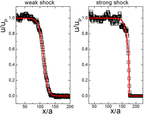
Figure 5: Typical shock profiles for a) weak shock and b) strong shock. The continuous lines represent phenomenological fits.

We conclude that by controlling $\delta_{0}$ or $P$, which parameterize the distance to the jamming point (at $P=0$ and $\delta_{0}=0$), we can tune $u_{P}^{*}$ and the onset of the strongly non-linear response of the packings. Our key numerical findings on the shock velocity summarized in Fig. 4 can be grasped from scaling near the jamming point.

III.4 Shock’s shape and width

Figure 5 shows typical shock profiles observed for weak and strong shock waves. In general, there are two main significant changes in the profiles due to the increase in the non-linearity of the phenomena. First, the width of the shocks decreases when increasing the non-linearity. Second, while symmetric profiles are obtained for weak shocks, strong shocks are associated with much more asymmetric profiles. Here we found that in all these cases, the profile of the shocks can be well approximated through the phenomenological expression:

$$u(X)=\frac{u_{p}}{1+\sum_{i}exp[p_{i}\,(X-X_{0})]}$$ (5)

where $u_{p}$ is the compression velocity, $X_{0}$ is the position of the shock wave, and the $p_{i}^{\prime}s$ are fitting parameters necessary to describe the profile Gomez . While in general weak (symmetric) shock profiles are well described by only one parameter $p_{1}$, the description of strong shocks requires at least three fitting parameters $p_{1}$-$p_{3}$. The continuous lines of Fig. 5 shows typical fits for weak and strong shocks.

In order to characterize the features of the shock profiles as a function of non-linearity, we systematically measure shock widths and symmetries for the different compression velocities, on systems with varying initial pressure. We define the shock’s width $\Delta$ and asymmetry parameter $Q$ by the expression Grad ,Torrilhon :

$$\Delta = \frac{u_{p}}{max(\frac{\partial u}{\partial x})}$$ (6)

$$Q = \frac{Q_{2}}{Q_{1}}=\frac{\int_{x^{*}}^{\infty}u(x)\,dx}{\int_{-\infty}^{x^{*}}[u_{p}-u(x)]\,dx}$$ (7)

where $x^{*}$ is such that $u(x^{*})=u_{p}/2$. Figure 6a shows a schematic of the shock profile illustrating the physical meaning of these definitions.

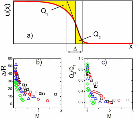
Figure 6: Shape characterization of the shock profiles. a) Scheme of the definition of shock’s width and asymmetry. Variation of shock width (b) and asymmetry (c) with the Mach number for the different studied shocks. The color code is the same as in figure 4.

Figures 6b and 6c show the results of shock’s width and asymmetry, as a function of the Mach number of the shocks. The width and symmetry of the shocks monotonically decrease as the nonlinearity increases. Note that while the width reaches 50 particles for weak shocks, it reduces to approximately 10 particles for strong shocks. Also it is clear that weak shocks are rather symmetric ($Q\sim 1$) and strong shocks are asymmetric $Q<1$ due to the slow relaxation behind the front.

III.5 Characterization of the shocked state

We have seen how the passage of the pressure front produces a transition in the granular media from an initial state to a different shocked state. Since the width of the shock waves is generally small, the shock compression process is usually considered to be a fast adiabatic transition Courant -MeyersBook ; this allows one to trace out the adiabatic equation of state by measuring the properties of shocks.

Generally, the features of the compressed region are studied through the shock adiabat, or Hugoniot curve, which is the locus of final shocked states. The Hugoniot is an adiabatic line in the $P-V$ plane (see Fig. 7a). Each point in this curve indicates the volume and pressure in the medium in the final shocked states. Note that during the compression experiment, which induces the transition from an initial state $(V_{0},P_{0})$ before the shock to a final state $(V_{S},P_{S})$ after the shock has passed, the system does not follow the Hugoniot curve in the intermediate states. In general the evolution is given by the Rayleigh line which is the straight line connecting initial and final states in the $P-V$ plane (see Fig. 7a).

As the shock compression process is adiabatic, the Hugoniot curve is often used to construct the equation of state of a given material. Following this idea, shock compression experiments have been designed and used for years to study the equation of state of solids and minerals at high pressures MeyersBook .

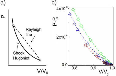
Figure 7: a) Schematic of a general shock Hugoniot curve (shock adiabat). b) Numerically obtained shock Hugoniot for systems with different initial pressures as obtained from the jump conditions. Dashed lines are guides to the eyes.

In our case the shock Hugoniot can be directly obtained from the simulations (by direct inspection of the final shocked states), or by using the Rankine-Hugoniot jump conditions. The conservation of mass and momentum across the shock front Eq. 3, can be rewritten relating the pressure and volume in the material with the particle and front velocities Courant -MeyersBook :

$$\begin{cases}V/V_{0}=1-u_{P}/v_{S}\\ P-P_{0}=\rho_{0}\,u_{P}\,v_{S}\\ \end{cases}$$ (8)

When the front velocity is known as a function of particle velocity $v_{S}=v_{S}(u_{P})$, these relations become an implicit expression for the Hugoniot curve. Figure 7b shows the shock Hugoniot curve as obtained by using the Rankine-Hugoniot conditions. In what follows, we use this numerically determined Hugoniot adiabat to study the stability of the shock waves for the case of small disturbances in the shape of the shock front.

III.6 Shock’s stability, roughness, and focusing

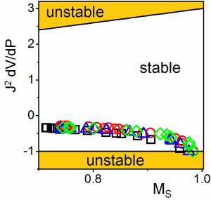
Figure 8: Dyakov’s stability analysis. Note that all the shock waves belong to the stable region of the phase diagram.

The stability of shock waves against shape perturbations has been one of the interesting and important topics of compressible flow. The theoretical investigations on this topic started with the seminal work of Dyakov Dyakov , based on a normal mode expansion of the front perturbations, later re-examined and presented in more detail by Swan and Fowles Swan .

Dyakov performed a linear stability analysis obtaining conditions for shock stability under which a shock wave remains stable, and front perturbations decreases exponentially in time. In this analysis the stability of the shocks is related with the slope of the Hugoniot adiabat, such that a shock wave remains stable whenever these conditions hold Dyakov , Swan :

$$\begin{cases}j^{2}dV/dP<1+2M_{S}\\ j^{2}dV/dP>-1\end{cases}$$ (9)

In these expressions the derivatives are taken along the Hugoniot adiabat, $M_{S}$ is the Mach number of the shock respect to the material behind the front, and $j^{2}$ is the slope of the Rayleigh line. In general, when the lower limit of the above equation is not satisfied the shock wave splits into two waves travelling in the same direction (splitting instability). The upper limit corresponds to the corrugation instability, where front modulations are exponentially amplified.

Note the simplicity and generality of this result. Once the Hugoniot curve is known these conditions are general and can be applied to any material. By using our numerically obtained shock Hugoniot, we can perform the Dyakov test stability analysis. Figure 8 shows our results, which suggest that the shock waves studied in this work are stable for the broad range of compressions and impact intensity analyzed.

Although the shock waves are stable, the disorder of the granular packings induce the roughening of the front (compare the fronts of Fig. 1 with Fig. 3a). In general, in crystalline solids shock front’s may also become irregular when travelling through poly-crystalline structures. Although not a proper instability, changes in the speed of sound with the lattice orientation can induce the corrugation and roughening of the shock front Meyers ,BarberKadau . In the amorphous structures considered here, the complete lack of symmetry produces a rather isotropic speed of sound such that irregularities in the front are restricted to a few particles diameters.

In order to analyze variation in front roughnesses we define the average front position $\langle x\rangle$ and roughness $\Delta x$ as:

$$\begin{cases}\langle x\rangle=\langle x_{0}(y)\rangle\\ \Delta x=\langle(x_{0}(y)-\langle x\rangle)^{2}\rangle^{1/2}\end{cases}$$ (10)

where $x_{0}(y)$ is the position of the front at $y$ (see Fig. 9a). Figure 9b shows the time evolution of the front roughness for shocks of varying Mach number. Interestingly, although the roughness of the fronts seems to reach maximum values less than $5-6$ particles, the value of the plateaus clearly depends on the nonlinearity of the wave. In particular, our simulations suggest that the more pronounced the nonlinearity of the wave is, the less rough its front is.

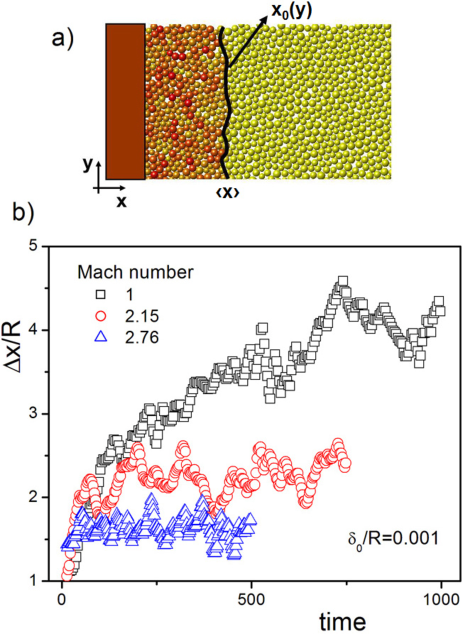
Figure 9: Evolution of the front’s roughess as a function of time for different Mach numbers. Note that when the nonlinearity of the wave is large, the roughness reaches a plateau at a small value.

IV Analytical theory of the Shock Speed

In this section, we analytically describe the relation between the shock speed and strength, shown in Fig. 4, using the jump conditions Eq. 3. Appendix B gives an alternative derivation. The first two equations can be used to predict the speed of the shock if we assume that the pressure is given entirely by the elastic forces between the particles. We describe the system with a one-dimensional one; then any interface cuts only one pair of particles from each other, and the pressure is just identical to the force between these two particles, and is given by Hertz’s law, $P=\epsilon\delta^{\alpha-1}$. Combining this equation of state with the expression for the density $\rho=\frac{M}{2R-\delta}$, the mass and momentum conservation conditions (first two relations in Eq. 3) imply:

$$\frac{v_{S}}{c_{0}}=\sqrt{\frac{1}{\alpha-1}\,\frac{(\delta_{S}/\delta_{0})^{\alpha-1}-1}{\delta_{S}/\delta_{0}-1}},$$ (11)

where $c_{0}$ represents the speed of sound before the passage of the shock wave. Together, Eqs. 4 and 11 can be seen as a parametric relation between front and particle velocities, where the overlap $\delta_{S}$ produced by the passage of the front is the parameter. Such a parametric plot of $v_{S}$ versus $u_{P}$ is drawn as a continuous line on the numerical data in Fig. 4b. This comparison shows that Eqs. 4 and 11 are in excellent agreement with the results of our numerical experiments on shock propagation.

Despite the good agreement with the numerical results, the third jump condition is not satisfied if we assume the previous expressions for $v_{S}$, $u_{P}$, and energy density per unit length $U=\epsilon\delta^{\alpha}\frac{\rho}{M}$ according to Hertz’s law. In the simulations the particles also have a random motion superimposed on the average velocity $u_{P}$. This produces an excess in the pressure and energy of the particles. In this case, the internal energy has an additional contribution, which can restore conservation of energy. More precisely, the random motion is described by an effective temperature $T_{S}$, and hence the speed of the shock is no longer overdetermined by the three jump conditions because the total number of unknowns, $v_{S}$, $\delta_{S}$ and $T_{S}$ is now equal to the number of conditions.

These heating effects should change the shock speed, but not drastically. The prediction above was based entirely on conservation of mass and momentum, which must still hold. However, the pressure will have a contribution from the thermal motion, and this can affect the conclusion. To estimate how big of an effect the thermal motion has, let us estimate how much energy is dissipated. First, the velocities may be eliminated from the three conservation laws to give:

$$\frac{\rho_{0}U_{S}-\rho_{S}U_{0}}{\rho_{S}-\rho_{0}}=\frac{P_{0}+P_{S}}{2}$$ (12)

(this is obtained by solving for the velocities from the first two conservation laws and substituting into the third). Taking $P_{0}$, $P_{S}$ and $U_{0}$ to have approximately the Hertzian form (i.e., neglecting the temperature), we can solve for $U_{S}$. The excess over the Hertzian potential energy, $\frac{\rho_{S}\delta_{S}^{\alpha}}{M\alpha}$ is then the thermal energy, which can be expressed entirely in terms of $\delta_{0}$ and $\delta_{S}$:

$$U_{thermal}=\frac{\frac{\varepsilon}{2}(\delta_{0}^{\alpha-1}+\delta_{S}^{\alpha-1})(\delta_{S}-\delta_{0})-\frac{\varepsilon}{\alpha}(\delta_{S}^{\alpha}-\delta_{0}^{\alpha})}{2R-\delta_{S}}.$$ (13)

When $\alpha$ is close to $2$, this energy excess becomes insignificant since this expression approaches $0$. In particular, when $\delta_{0}=0$ and $\alpha=\frac{5}{2}$, $U_{thermal}$ is $\frac{\alpha-2}{4}=\frac{1}{8}$ of the potential energy, explaining why our approximation agrees well with the numerics.

To summarize, the speed of a shock as a function of the compression can be estimated from conservation laws if one neglects the heating of the particles. In the limit where $\alpha$ is close to $2$ (as in the Hertzian case) this approximation is quite accurate.

One could go beyond this approximation and determine the exact relation between speed and compression in a shock. First the thermal contribution to both pressure and energy has to be predicted as a function of temperature. All the parameters of the shock can then be determined by solving all three jump conditions simultaneously.

V Conclusions

In this work, we have used simulations of piston compression experiments to unveil the mechanism of energy transport in granular systems composed of soft frictionless spheres. While at high confining pressures the elastic response of the granular system is basically linear, the low pressure regime is found to be dominated by non-linearities. Thus, for low confining pressures, when the system is close to the jamming-unjamming transition, the basic elastic excitations are supersonic shock waves, rather than linear phonons.

We have presented a detailed characterization of the weakly and strongly non-linear shocks, studying their propagation speed, width, shape, and stability. It is interesting to note that the propagation speed of shocks does not depend on friction or dissipation. Thus, experiments should focus on this quantity which is only affected by the contact interaction law. In general, the presence of friction or dissipation will affect other features like the width of shocks.

Finally, we developed a mathematical model that correctly captures the universal nonlinear response of granular packings around the jamming-unjamming transition. In particular, we have used this model to describe the dependence of the propagation speed on pressure and driving.

We conclude by saying that the elastic response of granular matter present unique features, not found in other condensed matter systems like solids, liquids, or gases. The athermal character of these systems allows the attainment of a state with zero pressure at non-vanishing density, the jamming point, which corresponds to a sonic vacuum. In this state the response of the system is characterized by a complete lack of linear behavior. Here we have shown how this fully nonlinear state also controls the elastic response of granular system in the low pressure regime.

Acknowledgments We acknowledge helpful discussions with M. van Hecke, V. Nesterenko, and D. A. Vega. This work was supported by FOM, Shell, the National Research Council of Argentina (CONICET), Universidad Nacional del Sur, and the Instituto de Física del Sur.

Appendix A Equation of motion

The Lagrangian of a $1d$ chain composed of soft spheres with repulsive interactions, as in Eq. 1, reads:

$$L=\sum_{n}\frac{1}{2}\,m\,\dot{\psi}_{n}^{2}-\frac{\varepsilon}{\alpha}(\psi_{n}-\psi_{n+1})^{\alpha},$$ (14)

where $\psi_{n}$ is the displacement of the $n$ particle, $m$ is the mass, $\varepsilon$ the interaction’s constant, and $\alpha$ the interaction’s exponent ($\alpha=5/2$ for Hertzian interactions). The continuum limit of the system is obtained by considering the limit where the radius of the spheres $R\rightarrow 0$. This limit is justified when the wavelength of waves is large compared to the size of the spheres. (As Nesterenko found, the wavelength is actually a fixed multiple of the size of the spheres, but the multiple is large enough that the continuum approximation is justified.) Here we proceed to replace the $\psi_{n}$’s by a continuous function and perform the continuum approximation in the Lagrangian, before deriving the equation of motion.

We first define a continuous function $\phi$ interpolating through the $\psi_{n}$’s. Although the most obvious choice is $\phi(2Rn)=\psi_{n}$, it is not the easiest to implement. In this case we have $\psi_{n}-\psi_{n+1}=-2R\phi^{\prime}(x)-2R^{2}\phi^{\prime\prime}(x)-\dots$ where $x=2Rn$ is the equilibrium position of the n^th sphere. Thus, this approximation will complicate the calculation of the potential energy, because we need to use the binomial theorem to raise $\psi_{n}-\psi_{n+1}$ to the $\alpha^{\mathrm{th}}$ power.

In order to get a simpler equation we take the continuum limit differently. Define $\phi$ by prescribing its derivative instead:

$$\psi_{n+1}-\psi_{n}=2R\phi^{\prime}(2R(n+\frac{1}{2}))\,$$ (15)

In this case the calculation of the potential energy will be simple, while the kinetic energy will receive corrections from an expansion in powers of $R$. (In Nesterenko’s version of the equation, dispersion effects appeared in the potential term so they were nonlinear and more complicated.) We first invert Eq. (15) in order to express $\psi_{n}$ in terms of $\phi$. To do that we make a Taylor expansion of the left-hand- side about $n+\frac{1}{2}$. This gives (up to terms of order $(2R)^{4}$):

$$\psi^{\prime}(2R(n+\frac{1}{2}))+\frac{(2R)^{2}}{24}\psi^{\prime\prime\prime}(2R(n+\frac{1}{2}))=\phi^{\prime}(2R(n+\frac{1}{2})).$$ (16)

Integration of both sides with respect to $x$ leads to $\phi(x)=(1+\frac{R^{2}}{6}\frac{d^{2}}{dx^{2}})\psi(x)$. Solving for $\psi$ in terms of $\phi$ gives:

$$\psi(x)=\frac{1}{1+\frac{R^{2}}{6}\frac{d^{2}}{dx^{2}}}\phi(x).$$ (17)

Expanding the ratio in a geometric series leads to $\psi(x)\approx\phi(x)-\frac{R^{2}}{6}\phi^{\prime\prime}(x)\dots$. Thus the kinetic energy term can be approximated by:

$$\frac{1}{2}\dot{\psi}_{n}^{2}\approx\frac{1}{2}\dot{\phi}(x)^{2}-\frac{R^{2}}{6}\dot{\phi}(n)\dot{\phi}^{\prime\prime}(x)$$ (18)

The approximated continuum Lagrangian is obtained by replacing the $\psi$ in terms of $\phi$ and the sum by an integral:

$$L\approx\int\left(\frac{1}{2}\dot{\phi}^{2}-\frac{R^{2}}{6}\dot{\phi}\dot{\phi}^{\prime\prime}-\frac{\varepsilon(2R)^{\alpha}}{m\alpha}(-\phi^{\prime})^{\alpha}\right)\frac{dx}{2R}$$

$$\approx\int\left(\frac{1}{2}\dot{\phi}^{2}-\frac{R^{2}}{6}(\dot{\phi}^{\prime})^{2}-\frac{\varepsilon(2R)^{\alpha}}{m\alpha}(-\phi^{\prime})^{\alpha}\right)\frac{dx}{2R}.$$

(19)

Finally, by using the Euler-Lagrange equation, we obtain the equation of motion:

$$\ddot{\phi}-\frac{R^{2}}{3}\,\ddot{\phi}^{\prime\prime}+\frac{\varepsilon(2R)^{\alpha}}{m}[(-\phi^{\prime})^{\alpha-1}]\,^{\prime}=0$$ (20)

In terms of the compression field $\delta=-2R\phi^{\prime}$ this equation takes the form:

$$\ddot{\delta}-\frac{R^{2}}{3}\,\ddot{\delta}^{\prime\prime}-\frac{4R^{2}\varepsilon}{m}\,[\delta^{\alpha-1}]\,^{\prime\prime}=0$$ (21)

This equation is simpler to the equation originally derived by Nesterenko; there is more than one way to take the continuum limit when the wavelength is the same order as the particle spacing. Here we found that this simpler equation is enough to describe the simulation results.

Appendix B Steady state solutions

The travelling of stationary perturbations having a propagation velocity $v_{S}$ can be considered by replacing the ansatz $\delta(x,t)=\delta(\tilde{t}\equiv t-\frac{x}{v_{S}})$ in the equation of motion. This function $\delta(\tilde{t})$ describes what an observer at a fixed point of space sees as the shock passes by. It satisfies the ordinary differential equation:

$$\frac{R^{2}}{3v_{S}^{2}}\,\frac{d^{4}\delta}{d\tilde{t}^{4}}-v_{S}^{2}\frac{d\delta}{d\tilde{t}}+\frac{\varepsilon}{mv_{S}^{2}}\frac{d^{2}[\delta^{\alpha-1}]}{d\tilde{t}^{2}}=0$$

Integrating twice and applying the boundary conditions $\delta(\tilde{t}\rightarrow-\infty)=\delta_{0}$, $\dot{\delta}(\tilde{t}\rightarrow-\infty)=\ddot{\delta}(\tilde{t}\rightarrow-\infty)=0$, leads to the following expression:

$$\frac{R^{2}}{3v_{S}^{2}}\,\ddot{\delta}-\delta+\frac{4\varepsilon R^{2}}{mv_{S}^{2}}\delta^{\alpha-1}=-\delta_{0}+\frac{4\varepsilon R^{2}}{mv_{S}^{2}}\delta_{0}^{\alpha-1}$$

This last equation can be rewritten in the form:

$$\frac{d^{2}\delta}{d\tilde{t}^{2}}=-\frac{dW}{d\delta},$$ (22)

where the field $W$ is given by:

$$\begin{split}W(\delta,v_{S})&=\frac{12\varepsilon}{m\alpha}\,(\delta^{\alpha}-\delta_{0}^{\alpha})-\frac{3v_{S}^{2}}{2R^{2}}(\delta-\delta_{0})^{2}\\ &-\frac{12\varepsilon}{m}\delta_{0}^{\alpha-1}(\delta-\delta_{0}).\end{split}$$ (23)

Thus, the problem of traveling steady waves is mapped to the motion of an effective particle moving (in time $\tilde{t}$) in a potential field $W$. Note that in this case the potential not only depends on the compression $\delta$, but also on the propagation speed $v_{S}$.

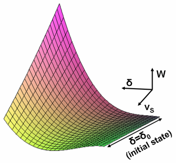
Figure 10: Effective potential surface. For $v_{S}>c$ the initial state becomes a local maxima allowing the description of travelling perturbations.

We now use this analogy to study the properties of travelling waves. Figure 10 shows the shape of the potential as a function of compression and propagation speed. In the initial state, the system is undistorted ($\delta=\delta_{0}$) and the effective particle is located at the extreme $W(\delta_{0},v_{s})=0$, at rest. For the cases where this initial state is a local minima, the effective particle remains at this initial position for all times. This means that in these cases steady perturbations cannot travel through the system. Thus, in order to describe travelling perturbations the initial state needs to be a local maximum such that $W_{\delta\delta}(\delta_{0},v_{S})<0$, and the speed of propagation needs to satisfy:

$$v_{S}^{2}\geq\frac{4R^{2}(\alpha-1)\varepsilon}{m}\delta_{0}^{\alpha-2}$$ (24)

Physically, this condition means that travelling perturbations will propagate at the speed of sound of the medium $c_{0}=2R\sqrt{(\alpha-1)\varepsilon/m}\,\delta_{0}^{\frac{\alpha-2}{2}}$, or faster. Figure 10 shows the change in the nature of the initial state, from a local minima to a local maxima, as the speed of propagation of the waves is increased.

B.1 Solitary waves

Now consider a travelling perturbation which satisfies the above condition ($v_{S}\geq c_{0}$). Figure 11a shows the shape of the potential $W(\delta)$ for a given front velocity $v_{S}$. Far away, the undistorted system corresponds to the effective particle located at the maxima of the potential $W=0$. The distortion induced by the passage of the wave can be seen as the particle rolling down the potential. The effective particle will move up to the turning point, and then the conservation of energy implies that the particle would roll back to the initial state.

This motion of the effective particle corresponds to a solitary wave travelling trough the system with velocity $v_{S}$ (Fig. 11b). Note that these solitary waves are the only steady state solutions of the system. The speed of propagation can be obtained from the turning point condition $W(\delta_{SOL},v_{S})=0$, where $\delta_{SOL}$ is the maximum compression due to the passage of the wave:

$$\frac{v_{S}}{c_{0}}=\sqrt{\frac{2}{\alpha(\alpha-1)}\left[\frac{\delta_{SOL}^{\alpha}-\delta_{0}^{\alpha}}{\delta_{0}^{\alpha-2}(\delta_{SOL}-\delta_{0})^{2}}-\frac{\alpha\delta_{0}}{\delta_{SOL}-\delta_{0}}\right]}$$ (25)

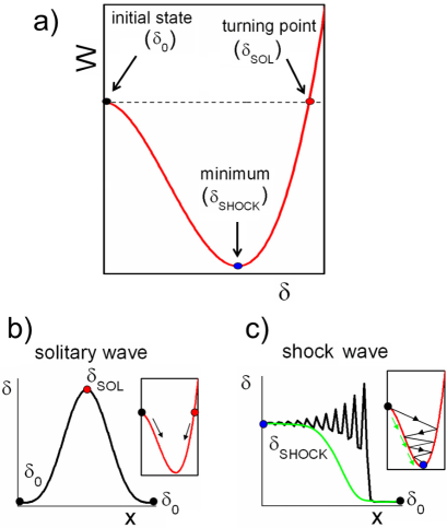
Figure 11: Steady state solutions of the non-linear wave equation. a) Potential well for a given propagation speed $v_{S}$. b) Solitary wave solutions obtained in te absence of viscosity. c) Shock wave solutions obtained for viscous dissipation.

B.2 Shock waves

The previous analysis shows that in the absence of any source of dissipation the motion of the effective particle conserves its energy, and the only steadily propagating solutions are solitary waves. In that case homogeneous shocks, as found through the simulations in this work, are not possible solutions of the equation of motion.

In order to obtain steady state shock solutions, some sort of dissipation is needed. In general, the effect of dissipation can be taken into account by adding new terms in equation 20. For example, if a dissipation term (due to relative motion of the spheres) is considered Herbold , the equation of motion of the system will take the form:

$$\ddot{\phi}-\frac{R^{2}}{3}\,\ddot{\phi}^{\prime\prime}+\frac{4R^{2}\varepsilon}{m}[(-\phi^{\prime})^{\alpha-1}]\,^{\prime}-4R^{2}\eta\dot{\phi}^{\prime\prime}=0,$$ (26)

where $\eta$ is a damping coefficient.

Now if we look for steady state travelling perturbations with the same procedure as before, we obtain the following equation:

$$\frac{d^{2}\delta}{d\tilde{t}^{2}}=-\frac{dW}{d\delta}-12\eta\frac{d\delta}{d\tilde{t}}$$ (27)

Here the potential $W$ is the same as obtained before (equation (23)). Thus, for this particular form of dissipation, we have explicitly shown that the problem of steadily propagating waves is mapped to the problem of an effective particle moving in a potential, but now the particle also moves under the effect of friction.

In this case, the presence of friction will take out the energy of the effective particle, inducing the oscillation to decay to the minimum of the potential well. These solutions correspond to oscillatory shock waves (Fig. 11c, black line).

If the viscosity is high enough, the motion of the effective particle will become overdamped, and the particle directly moves to the minimum of the potential, without performing any oscillation. This motion corresponds to traveling regular shock profiles (Fig. 11c, green line).

For the shock waves the relation between propagation velocity and induced compression can be obtained by the condition $\frac{dW}{d\delta}_{\mid\,\delta_{S},v_{S}}=0$, which corresponds to the minimum of the potential. This condition leads to:

$$\frac{v_{S}}{c_{0}}=\sqrt{\frac{1}{\alpha-1}\,\frac{(\delta_{S}/\delta_{0})^{\alpha-1}-1}{\delta_{S}/\delta_{0}-1}},$$ (28)

where $\delta_{S}$ is the maximum compression after the shock wave has passed. In Sec. IV, imposing two of the jump conditions (conservation of momentum and mass, but not energy) produced the same result. The dissipation term we have added preserves the same two conservation laws, explaining the agreement. In Sec. IV, we justified the disappearance of energy not by introducing friction (since the simulations did not include it) but by assuming that the energy is converted to random motion of the particles. A more accurate treatment of this hypothesis would have to account for some additional thermal pressure.

References

- (1) A. Mehta, Granular Physics (Cambridge University Press, Cambridge, 2007).
- (2) H. M. Jaeger, Sidney R. Nagel, and R. P. Behringer, Rev. Mod. Phys. 68, 1259 (1996).
- (3) X. Jia, C. Caroli, and B.Velicky, Phys. Rev. Lett. 82, 1863 (1999).
- (4) B. Gilles and C. Coste, Phys. Rev. Lett. 90, 174302 (2003).
- (5) H. A. Makse, D. L. Johnson, and L.M. Schwartz, Phys. Rev. Lett. 84, 4160 (2000).
- (6) X. Jia, Phys. Rev. Lett. 95, 154303 (2004).
- (7) D. J. Durian, Phys. Rev. Lett. 75, 4780 (1995).
- (8) C. S. O’Hern, L. E. Silbert, A. J. Liu, and S. R. Nagel, Phys. Rev. E 68, 011306 (2003).
- (9) M. van Hecke, J. Phys.: Condens. Matter 22, 033101 (2010).
- (10) L. M. Schwartz, D. L. Johnson, and S. Feng Phys. Rev. Lett. 52, 831 (1984).
- (11) C. S. O’Hern, S. A. Langer, A. J. Liu, and S. R. Nagel, Phys. Rev. Lett. 88, 075507 (2002).
- (12) L. E. Silbert, A. J. Liu, and S. R. Nagel, Phys. Rev. Lett. 95, 098301 (2005).
- (13) M. Wyart, S. R. Nagel, and T. A. Witten, Europhys. Lett. 72, 486 (2005).
- (14) M. Wyart, L E. Silbert, S. R. Nagel, and T. A. Witten Phys. Rev. E 72, 051306 (2005).
- (15) E. Somfai, J. N. Roux, J. H. Snoeijer, M. van Hecke, and W. van Saarloos, Phys. Rev. E 72, 021301 (2005).
- (16) W. G. Ellenbroek, E. Somfai, M. van Hecke, and W. van Saarloos, Phys. Rev. Lett. 97, 258001 (2006).
- (17) N. Xu, V. Vitelli, M. Wyart, A. J. Liu, and S. R. Nagel, Phys. Rev. Lett. 102, 038001 (2009).
- (18) A. Souslov, A. J. Liu, and T. C. Lubensky, Phys. Rev. Lett. 103, 205503 (2009).
- (19) N. Xu, V. Vitelli, A. J. Liu, and S. R. Nagel, Europhys. Lett. 90, 56001 (2010).
- (20) V. Vitelli, N. Xu, M. Wyart, A. J. Liu, and S. R. Nagel, Phys. Rev. E 81, 021301 (2010).
- (21) B. P. Tighe, Phys. Rev. Lett. 107, 158303 (2011).
- (22) V. F. Nesterenko, J. Appl. Mech. Tech. Phys. 5, 733 (1984).
- (23) V. F. Nesterenko, Dynamics of Heterogeneous Materials (Springer-Verlag, New York, 2001).
- (24) R. S. Sinkovits and S. Sen, Phys. Rev. Lett. 74, 2686 (1997).
- (25) C. Coste, E. Falcon, and S. Fauve, Phys. Rev. E 56, 6104 (1997).
- (26) C. Daraio, V. F. Nesterenko, E. B. Herbold, and S. Jin, Phys. Rev. E 72, 016603 (2005).
- (27) S. Job, F. Melo, A. Sokolow, and S. Sen, Granular Matter 10, 13 (2007).
- (28) S. Sen, J. Hong, J. Bang, E. Avalos, and R. Doney, Physics Reports 462, 21 (2008).
- (29) L. R. Gómez, A. M. Turner, M. van Hecke, and V. Vitelli, Phys. Rev. Lett. 108, 058001 (2012).
- (30) M. P. Allen and D. J. Tildesley, Computer Simulation of Liquids (Oxford University Press, Oxford, 1989).
- (31) R. Courant and K. O. Friedrichs, Supersonic Flow and Shock Waves(Springer-Verlag, Berlin, 1985).
- (32) Y. B. Zeldovich and Y. P. Raizer, Physics of Shock Waves and High Temperature Phenomena (Academic Press, New York, 1966), Vol. I, II.
- (33) M. A. Meyers, Dynamic Behavior of Materials (Wiley- Interscience, New York, 1994).
- (34) B. L. Holian, H. Flaschka, and D. W. McLaughlin, Phys. Rev. A 24, 2595 (1981).
- (35) E. M. Bringa, B. D. Wirth, M. J. Caturla, J. Stolken, and D. Kalantar, Nucl. Instr. and Meth. in Phys. Res. B 202, 56 (2003).
- (36) G. E. Duvall, R. Manvi, and S. C. Lowell. J. Appl. Phys. 40, 3771 (1969).
- (37) E. B. Herbold and V. F. Nesterenko, Phys. Rev E 75, 021304 (2007).
- (38) A. Rosas, A. H. Romero, V. F. Nesterenko, and K. Lindenberg. Phys. Rev. Lett. 98, 164301 (2007).
- (39) H. Grad, Commun. Pure Appl. Maths 5, 257 (1952).
- (40) M. Torrilhon and H. Struchtrup, J. Fluid Mech. 513, 171 (2004).
- (41) S. P. Dyakov, Zh. Eksp. Teor. Fiz. 27, 288 (1954).
- (42) G. H. Swan and G. R. Fowles, Phys. Fluids 18, 28 (1975).
- (43) M. C. Meyers. Materials Science and Engineering 30, 99 (1977).
- (44) J. L. Barber and K. Kadau, Phys. Rev. B 77, 144106 (2008)