Unitary quantum phase operators for bosons and fermions: A model study on quantum phases of interacting particles in a symmetric double-well potential

Abstract

We introduce unitary quantum phase operators for material particles. We carry out a model study on quantum phases of interacting bosons in a symmetric double-well potential in terms of unitary and commonly-used non-unitary phase operators and compare the results for different number of bosons. We find that the results for unitary quantum phase operators are significantly different from those for non-unitary ones especially in the case of low number of bosons. We introduce unitary operators corresponding to the quantum phase-difference between two single-particle states of fermions. As an application of fermionic phase operators, we study a simple model of a pair of interacting two-component fermions in a symmetric double-well potential. We also investigate quantum phase and number fluctuations to ascertain number-phase uncertainty in terms of unitary phase operators.

1 Introduction

The quantum phase of interacting systems plays an important role in describing a variety of physical phenomena such as phase transitions, superfluid tunnelling, Josephson effects etc. With advancement in precision interferometry with ultracold atoms [1, 2, 3] in confined geometries such as traps and atom chips, developing a proper understanding of the quantum phase properties of interacting particles is of prime interest. As far as quantum phase measurement and its theoretical interpretations are concerned, there are unresolved issues which need to be addressed, in particular in the context of emerging field of atom optics. For instance, a proper definition of ‘quantum phase’ of electromagnetic fields had remained a hotly debated topic in theoretical quantum physics for a long time [4, 5, 6, 7, 8]. Accurate determination of phase difference between two optical fields in the quantum domain remains an elusive task due to lack of theoretical understanding of quantum phases. It is also known that such a difficulty exists even in the case of semi-classical radiation theory when the field is weak and amplitude and phase fluctuations are correlated. About two decades ago, Mandel’s group [9, 10, 11, 12] experimentally examined two closely related but distinct measurement schemes for determining phase difference between two optical fields in both semi-classical and quantum cases. They made use of sine and cosine of phase-difference operators as defined by Carruthers and Nieto [7]. Furthermore, to resolve the problems associated with quantum phase measurement, Noh et al. [9, 11] introduced an operational definition of quantum phase that requires different phase operators for different measurement schemes.

Quantum phase problems for electromagnetic fields had been extensively studied during 90’s. However, to the best of our knowledge, quantum phase problem in the context of matter waves has not been addressed so far. Trapped ultracold atoms can be considered as an isolated interacting many-particle quantum system in the absence of any appreciable trap-loss. It is then necessary to formulate quantum phase of matter waves with fixed total number of particles. To introduce quantum phase operators for material particles, one has to distinguish between bosonic and fermionic matter. Unitary quantum phase operators for bosons are introduced following the existing quantum phase operator formalism of photons which are bosons. Quantum phase operators for fermions are not known. It is difficult to define a unitary quantum phase operator for fermions by a simple extension of the existing quantum phase formalism of photons, because unlike photons, more than one fermion can not occupy a single quantum state.

Here we introduce unitary and Hermitian quantum phase operators corresponding to the phase-difference between two single-particle quantum states in terms second quantised fermionic operators. A quantum state for fermions can be either filled (by one fermion) or empty (vacuum state). The unitarity of the operators is ensured by coupling the filled state with the vacuum. Therefore, quantum phase-difference between two fermionic modes becomes well defined when single-particle quantum states of fermions are half filled. To understand the underling features of quantum phases of interacting fermionic or bosonic particles, we resort to a simple microscopic model of 1D symmetric double-well potential. In case of two particles, this model enables us to work with an analytical solution. In order to elucidate canonically conjugate nature of number-difference and phase-difference operators, we apply our formalism to study quantum fluctuations of both number- and phase-difference operators. One can introduce two non-commuting operators corresponding to the cosine and sine of the phase-difference operators. Both of them are canonically conjugate to the number-difference operators. These two phase operators plus the number-difference operator form a closed algebra. A unitary and hermition phase-difference operator and corresponding phase-difference state can be constructed using the cosine and sine phase-difference operators.

We find that for low number of bosons, the phase properties calculated with unitary phase-difference operators are significantly different from those calculated with non-unitary Carruther-Nieto phase-difference operators. However, for large number of bosons the results tend to converge. Since unitarity of phase operators is ensured by coupling vacuum state with the highest number state in a finite dimensional Fock space, the effects of vacuum state on quantum phase properties is found to be quite substantial in case of low number of bosons. Since the operator corresponding to the number-difference between the two modes is canonically conjugate to the phase-difference operator, we also study the fluctuation of number-difference to ascertain number-phase uncertainty and non-classical behaviour in quantum phase dynamics. In case of fermions, we investigate fluctuations in phase-difference and number-difference of a pair of two-component interacting fermions.

This paper is organised in the following way. In section $2$, we introduce unitary quantum phase operators of bosons as well as fermions and discuss in some detail the unitarity of quantum phase operators. We describe hamiltonian dynamics of a few interacting bosons or fermions in a 1D symmetric double-well potential in section 3. In section 4, we present and analyse numerical results on quantum phases, number- and phase-fluctuations of different number of bosons in in the double-well potential. For fermions, we study numerically only the case of a pair of two-component fermions and compare the results with those of a pair of bosons. We conclude this paper in section $5$.

2 Quantum Phase Operators

Here we present operator formalism for quantum phases of bosons and fermions. For bosons, a proper quantum mechanical phase operator can be defined following that for quantised radiation fields. For fermions, there exists no standard definition of a proper quantum mechanical phase operator. We here introduce a unitary phase operator for fermions. Before we discuss our new formalism, let us have a revisit into the history of quantum phase problem.

In classical mechanics, amplitude and phase are two canonically conjugate variables which appear in the expression of displacement $x_{\mu}(t)=2A_{\mu}\cos(\phi_{\mu}-\omega_{\mu}t)$ of classical field of $\mu$-th mode. This can be rewritten as

$$x_{\mu}(t)=2A_{\mu}\cos(\phi_{\mu}-\omega_{\mu}t)=A_{\mu}\left[e^{i\phi_{\mu}}e^{-i\omega_{\mu}t}+e^{-i\phi_{\mu}}e^{i\omega_{\mu}t}\right]$$ (1)

where $A_{\mu}$ and $\phi_{\mu}$ are the amplitude and phase of the $\mu$-th mode of the field and $\omega_{\mu}$ represents a harmonic frequency. In quantum mechanics, $x_{\mu}(t)$ is replaced by the operator

$$\hat{x}_{\mu}(t)=x_{\mu 0}\left[\hat{a}_{\mu}e^{-i\omega_{\mu}t}+\hat{a}_{\mu}^{\dagger}e^{i\omega_{\mu}t}\right]$$ (2)

where $\hat{a}_{\mu}(\hat{a}_{\mu}^{\dagger})$ represents the annihilation (creation) operator of a quanta of the quantised field in $\mu$-th mode. A comparison between the equations (1) and (2) suggests that in the classical limit $\hat{a}_{\mu}\rightarrow A_{\mu}e^{i\phi}$. Assuming that there exists a Hermitian phase operator $\hat{\phi}_{\mu}$ which is canonically conjugate to the number operator $\hat{N}_{\mu}=\hat{a}_{\mu}^{\dagger}a_{\mu}$, classical limit of such a phase operator may be attained by making use of the coherent state description of quantised fields. In classical mechanics, the azimuthal angle $\phi$ is given by

$$\phi=\tan^{-1}(y/x)$$ (3)

and defines a modulo of $2\pi$. Now, defining $\phi$ to be continuous in $-\infty<\phi<\infty$, the angular momentum $L_{z}$ in three dimension is given by

$$L_{z}=xP_{y}-yP_{x}=-i\hbar\frac{\partial}{\partial\phi}$$ (4)

where $P_{x}$ and $P_{y}$ are $x$- and $y$-component, respectively, of the momentum $P$. $L_{z}$ and $\phi$ are conjugate variables and they satisfy

$$[\phi,L_{z}]=i\hbar$$ (5)

$L_{z}$ is Hermitian in the space of periodic functions of period $2\pi$, but here $\phi$ is not periodic. Susskind and Glogower [6] showed that the non-periodicity of $\phi$ makes $\phi$ non-hermitian.

To define a phase operator in quantum mechanics is a delicate problem. The major difficulty in defining a proper phase operator is its non-unitarity which stems from the fact that the number operator of a harmonic oscillator has a lower bound in its eigenvalue spectrum. Dirac [4] first postulated the existence of a Hermitian phase operator in his description of quantised electromagnetic fields. Susskind and Glogower [6] first showed that Dirac’s phase operator was not unitary and hence not Hermitian. Using Dirac’s phase operator, if one tries to constructs a unitary operator $U$, then it turns out that, $UU^{\dagger}$ is an identity operator but $U^{\dagger}U$ is not an identity operator. Therefore, $U$ is not unitary. Thus Susskind and Glogower [6] concluded that since $U$ is not unitary there does not exist a Hermitian phase operator.

Louisell [5] first introduced the periodic operator function in defining a phase variable conjugate to the angular momentum. Carrauthers and Nieto [7] showed that one can define two Hermitian phase operators C and S corresponding to cosine and sine of the classical phase, respectively. However, these operators are non-unitary. Using these operators, they introduced two-mode phase difference operators of a two-mode radiation field. Explicitly, the two-mode phase-difference operators are defined as

$$\hat{C}_{12}^{\rm{CN}}=\hat{C}_{1}\hat{C}_{2}+\hat{S}_{1}\hat{S}_{2}$$

$$\hat{S}_{12}^{\rm{CN}}=\hat{S}_{1}\hat{C}_{2}-\hat{S}_{2}\hat{C}_{1}$$ (6)

where

$$\hat{C}_{i}=\frac{1}{2}((\hat{N}_{i}+1)^{-\frac{1}{2}}\hat{a}_{i}+\hat{a}_{i}^{\dagger}(\hat{N}_{i}+1)^{-\frac{1}{2}})$$ (7)

$$\hat{S}_{i}=\frac{1}{2i}(\hat{N}_{i}+1)^{-\frac{1}{2}}\hat{a}_{i}-\hat{a}_{i}^{\dagger}(\hat{N}_{i}+1)^{-\frac{1}{2}})$$ (8)

are the phase operators corresponding to sine and cosine, respectively, of the $i$-th mode. In terms of creation (annihilation) operator $\hat{a}_{i}^{\dagger}(\hat{a}_{i})$ of the corresponding modes ($i=1,2$), phase difference operator can be written as

$$\hat{C}^{\rm{CN}}_{12}=\frac{1}{2}[(\hat{N}_{1}+1)^{-\frac{1}{2}}\hat{a}_{1}\hat{a}_{2}^{\dagger}(\hat{N}_{2}+1)^{-\frac{1}{2}}+\hat{a}_{1}^{\dagger}(\hat{N}_{1}+1)^{-\frac{1}{2}}(\hat{N}_{2}+1)^{-\frac{1}{2}}\hat{a}_{2}]$$ (9)

$$\hat{S}^{\rm{CN}}_{12}=\frac{1}{2i}[(\hat{N}_{1}+1)^{-\frac{1}{2}}\hat{a}_{1}\hat{a}_{2}^{\dagger}(\hat{N}_{2}+1)^{-\frac{1}{2}}-\hat{a}_{1}^{\dagger}(\hat{N}_{1}+1)^{-\frac{1}{2}}(\hat{N}_{2}+1)^{-\frac{1}{2}}\hat{a}_{2}]$$ (10)

The above cosine and sine phase-difference operators are non-unitary. Pegg and Burnett [8] first introduced a Hermitian and unitary phase operator.

In the description of interference phenomena and interferometric experiments, we need to evaluate the phase-difference between two fields and not the absolute phase of a field. It is therefore practical to seek a Hermitian operator corresponding to phase-difference between two modes of a quantised field. By synthesizing the methods of Pegg-Burnett [8] and Carruthers-Nieto, Deb et al. [14] introduced Hermitian and unitary phase-difference operators of a two-mode field with fixed number of total photons. It is done by coupling the vacuum state of one mode with the highest Fock state of the other in finite dimensional Fock space. The cosine and sine phase-difference operators take form [15]

$$\hat{C}_{12}=\hat{C}^{\rm{CN}}_{12}+\hat{C}_{12}^{(0)}$$ (11)

$$\hat{S}_{12}=\hat{S}^{\rm{CN}}_{12}+\hat{S}_{12}^{(0)}$$ (12)

where

$$\hat{C}_{12}^{(0)}=\frac{1}{2}\left[|N,0\rangle\langle 0,N|+|0,N\rangle\langle N,0|\right]$$ (13)

$$\hat{S}_{12}^{(0)}=\frac{1}{2i}\left[|N,0\rangle\langle 0,N|-|0,N\rangle\langle N,0|\right]$$ (14)

describe the contributions from the vacuum states of the two modes. $|N_{1},N-N_{1}\rangle$ represents a two-mode Fock state with $N_{1}$ and $N-N_{1}$ being the photon numbers in mode 1 and 2, respectively. In case of quantised electromagnetic fields, the assumption of a fixed number of photons is made to circumvent the problem of non-unitarity. However, after all calculations are done one has to take the limit that the number of photons goes to infinity.

2.1 Unitary quantum phase operators for bosons

Since it is possible to keep the total number of particles in a double-well fixed in the absence of any loss, the assumption of a fixed total number of quanta (in this case, the total number of particles) is justified and not just for a calculational advantage as in electromagnetic fields. We consider that the two modes 1 and 2 correspond to the second quantized matter wave fields of the left and right well, respectively, of 1D double-well potential of equation (27). We further assume that the energy is low and the inter-particle interaction is weak so that a single boson remains in the lowest energy state with symmetric combination of the two harmonic oscillator ground states. Let the operators $\hat{a}_{i}(\hat{a}_{i}^{\dagger})$ represent annihilation (creation) operator of a particle in left ($i=1$ or right well ($i=2$) harmonic oscillator ground state. Then the operators defined in equations (5) and (6) suffice to be the two-mode phase-difference operators of bosons in a double-well potential corresponding to the cosine and sine, respectively, of the two-mode phase-difference. Thus we have $\hat{C}^{\rm{B}}_{12}\equiv\hat{C}_{12}$ and $\hat{S}^{\rm{B}}_{12}\equiv\hat{S}_{12}$ where the superscript $\rm{B}$ stands for boson. The difference of the number operators or the population imbalance between the two wells is $\hat{W}^{\rm{B}}=\hat{a}_{1}^{\dagger}\hat{a}_{1}-\hat{a}_{2}^{\dagger}\hat{a}_{2}$. The three operators $\hat{C}^{\rm{B}}_{12}$, $\hat{S}^{\rm{B}}_{12}$ and $\hat{W}^{\rm{B}}$ operators obey closed cyclic commutation algebra as follows

$$\left[[\hat{C}^{\rm{B}}_{12},\hat{S}^{\rm{B}}_{12}],\hat{W}^{\rm{B}}\right] + \left[[\hat{S}^{\rm{B}}_{12},\hat{W}^{\rm{B}}],\hat{C}^{\rm{B}}_{12}\right]+\left[[\hat{W}^{\rm{B}},\hat{C}^{\rm{B}}_{12}],\hat{S}^{\rm{B}}_{12}\right]=0$$ (15)

The commutation algebra of the given operators are following

$$\left[\hat{C}^{\rm{B}}_{12},\hat{W}^{\rm{B}}\right] = 2i\left(\hat{S}^{\rm{B}}_{12}-(N+1)\hat{S}^{{(0)}}_{12}\right)$$

$$\left[\hat{S}^{\rm{B}}_{12},\hat{W}^{\rm{B}}\right] = -2i\left(\hat{C}^{\rm{B}}_{12}-(N+1)\hat{C}^{(0)}_{12}\right)$$

One can define a unitary phase-difference operator [16]

$$\hat{\beta}_{12}=\hat{C}^{\rm{B}}_{12}+i\hat{S}^{\rm{B}}_{12}.$$ (17)

The eigenstate of this operator, that is, phase-difference state can be constructed as the product of single-mode phase states of Pegg-Burnett [8] subject to the condition that total number of quanta in the two modes is a constant of motion. The procedure for deriving phase-difference state is described in references [14, 15]. The important point to be noted here is that for low number of total bosons $N$, the effect of vacuum states such as $\mid 0,N\rangle$ and $\mid N,0\rangle$ on quantum phase-difference is quite significant as would be discussed in section 4. Therefore, in case of low $N$, one has to use unitary quantum phase-difference operators as defined in equation (17) for accurate measurement of quantum phases. The phase-difference operators of Carruthers and Nieto will approach unitarity in the limit $N\rightarrow\infty$. In a recent theoretical paper by Sarma and Zhou [17], an operator similar to that of Carrruthers and Nieto has been implicitly used for studying phase dynamics of a Bose-Einstein condensate (BEC) in a double-well. It is worthwhile to mention that while in case of BEC, probably a non-unitary phase operator such as used in [17] can suffice for phase measurement for all practical purpose, a few bosons in a double well necessarily require unitary phase difference operators for high precision phase measurement, in particular for the purpose quantum information processing with a few bosons in a double-well.

2.2 Unitary quantum phase operators for fermions

In the previous subsection, we have introduced phase operators for massive bosons with an analogy with the phase operators of electromagnetic fields of massless photons. This analogy has been possible because of bosonic symmetry in both the cases. Bosonic symmetry allows a large number of bosons to occupy a single-particle quantum state (or mode). For fermions, obviously such an analogy can not be drawn. A single-particle quantum state defined by a set of quantum numbers including spin magnetic quantum number can not be occupied by more than one fermion due to Pauli’s exclusion principle.

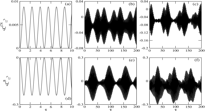
Figure 1: The top and bottom panels show the variation of average of the cosine phase-difference operator $\langle C^{\rm{CN}}_{12}\rangle$ and $\langle C^{\rm{B}}_{12}\rangle$, respectively, as a function of $\tau$ for $\bar{U}=0.05$. From left to right, subplots correspond to different number of bosons $N=2$ (a,d), $N=5$ (b,e) and $N=10$ (c,f) respectively.

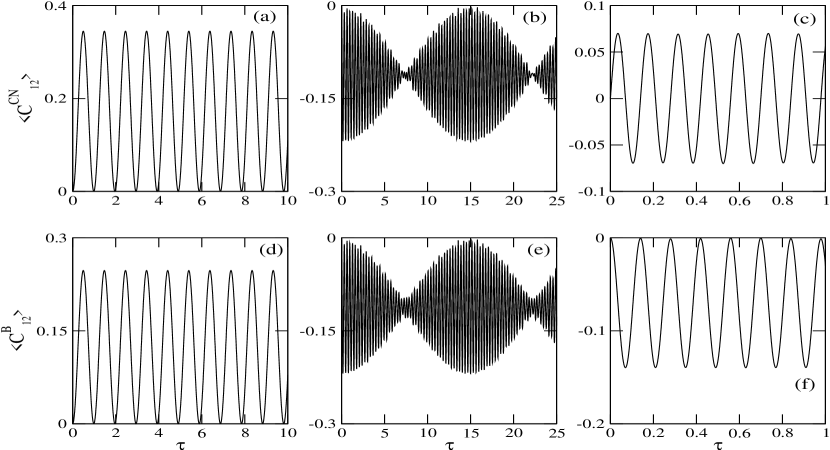
Figure 2: Same as in figure 1 but for $\bar{U}=5.0$. The subplots correspond to different number of bosons $N=2$ (a,d), $N=5$ (b,e) and $N=10$ (c,f) respectively.

Let us now discuss how we can introduce operators corresponding to the phase-difference between two single-particle fermionic quantum states or modes. If we construct a phase-difference operator between two fermionic modes following the method of Carruthers and Nieto, obviously such an operator will deviate largely from the unitarity since a fermionic mode can be occupied more than a single fermion. Let us write two hermition operators corresponding to the cosine and sine of phase-difference between two fermionic modes along the lines of Carrathers-Nieto phase formalism and check the usefulness of such operators. Two fermionic modes can be characterised by the the principal quantum numbers $n$ and $n^{\prime}$ of low lying harmonic oscillator states on the left and right well, respectively, and two spin degrees-of-freedom $\sigma$ and $\sigma^{\prime}$ on the left and right well, respectively. For simplicity, we assume that $n=n^{\prime}$ and suppress $n$-index. We then have the two modes $m\equiv l,\sigma$ and $m^{\prime}\equiv r,\sigma^{\prime}$. The cosine and sine phase-difference operators can be given by

$$\hat{C}_{mm^{\prime}} = \frac{1}{2}\left[(\hat{N}_{m}+1)^{-\frac{1}{2}}\hat{a}_{m}\hat{a}_{m^{\prime}}^{\dagger}(\hat{N}_{m^{\prime}}+1)^{-\frac{1}{2}}\right.$$ (18)

$$+ \left.\hat{a}_{m}^{\dagger}(\hat{N}_{m}+1)^{-\frac{1}{2}}(\hat{N}_{m^{\prime}}+1)^{-\frac{1}{2}}\hat{a}_{m^{\prime}}\right]$$

$$\hat{S}_{mm^{\prime}} = \frac{1}{2i}\left[(\hat{N}_{m}+1)^{-\frac{1}{2}}\hat{a}_{m}\hat{a}_{m^{\prime}}^{\dagger}(\hat{N}_{m^{\prime}}+1)^{-\frac{1}{2}}\right.$$ (19)

$$- \left.\hat{a}_{m}^{\dagger}(\hat{N}_{m}+1)^{-\frac{1}{2}}(\hat{N}_{m^{\prime}}+1)^{-\frac{1}{2}}\hat{a}_{m^{\prime}}\right]$$

Here the operators $a_{m}$ satisfy the anti-commutator algebra

$$\left\{a_{m},a_{m^{\prime\prime}}^{\dagger}\right\}=a_{m}a_{m^{\prime\prime}}^{\dagger}+a_{m^{\prime\prime}}^{\dagger}a_{m}=\delta_{mm^{\prime\prime}}\equiv\delta_{ss^{\prime\prime}}\delta_{\beta\beta^{\prime\prime}}\delta_{\sigma\sigma^{\prime\prime}}$$ (20)

$$\left\{a_{m},a_{m^{\prime\prime}}\right\}=a_{m}a_{m^{\prime\prime}}+a_{m^{\prime\prime}}a_{m}=0$$ (21)

$$\left\{a_{m}^{\dagger},a_{m^{\prime\prime}}^{\dagger}\right\}=a_{m}^{\dagger}a_{m^{\prime\prime}}^{\dagger}+a_{m^{\prime\prime}}^{\dagger}a_{m}^{\dagger}=0$$ (22)

and $\hat{N}_{m}=a_{m}^{\dagger}a_{m}$ is the number operator of the $m$-th mode. The total number of fermions $N=\sum_{m}\hat{N}_{m}$ is assumed to be a constant.

To construct an eigenstate of $\hat{C}_{mm^{\prime}}$ or $\hat{S}_{mm^{\prime}}$, we consider many-fermion basis states in all possible configurations of fermion distribution in all available low-energy single-particle states. For instance, let us denote such a basis state in the form $\mid 01\rangle_{i}\equiv\mid\{0\}_{m},\{1\}_{m^{\prime}}\rangle\otimes\mid\{(N-1)\}\rangle_{i}$ in $i$-th configuration in which $\mid\{0\}_{m},\{1\}_{m^{\prime}}\rangle$ implies 0 fermion in $m$-th mode and 1 fermion in $m^{\prime}$-th. The rest of the fermions ($N-1$) are distributed over all the modes except the two modes $m$ and $m^{\prime}$. The ket $\mid\{(N-1)\}\rangle_{i}$ represents a configuration of ($N-1$) fermions distributed over ($N_{s}-2$) modes. A general many-fermion state can be written as

$$\mid\psi\rangle = \sum_{i}d_{00}^{(i)}\mid 00\rangle_{i}+\sum_{j}d_{01}^{(j)}\mid 01\rangle_{j}+\sum_{k}d_{10}^{(k)}\mid 10\rangle_{k}+\sum_{l}d_{11}^{(l)}\mid 11\rangle_{l}$$ (23)

where $\mid nn^{\prime}\rangle_{i}\equiv\mid\{n\}_{m},\{n^{\prime}\}_{m^{\prime}}\rangle\otimes\mid\{(N-n-n^{\prime})\}\rangle_{i}$. The summation over the index $i$ implies sum over all the configurations in which $m$ and $m^{\prime}$ can be empty. Similarly summation over $j$, $k$ and $l$ imply sums over configurations of the types $\mid 01\rangle_{j}$, $\mid 10\rangle_{k}$ and $\mid 11\rangle_{l}$, respectively. From eigenvalue equation $\hat{C}_{mm^{\prime}}\mid\psi\rangle=C\mid\psi\rangle$ we infer that $d_{00}^{(i)}=0$ for all $i$, $d_{11}^{(l)}=0$ for all $l$ while $d_{01}^{(j)}$ and $d_{10}^{(k)}$ are in general nonzero. Now, using the operators of equations (18) and (19), one can construct an operator $\hat{U}_{mm^{\prime}}=\hat{C}^{\rm{F}}_{mm^{\prime}}+i\hat{S}^{\rm{F}}_{mm^{\prime}}=(\hat{N}_{m}+1)^{-\frac{1}{2}}\hat{a}_{m}\hat{a}_{m^{\prime}}^{\dagger}(\hat{N}_{m^{\prime}}+1)^{-\frac{1}{2}}$. Assuming a phase-difference state of the form $\mid\psi_{mm^{\prime}}\rangle=\sum_{i}d_{01}^{(i)}\mid 01\rangle_{i}+\sum_{k}d_{10}^{(j)}\mid 10\rangle_{j}$ with $\sum_{i}|d_{01}^{(i)}|^{2}+\sum_{j}|d_{10}^{(j)}|^{2}=1$, we find $\langle\psi_{mm^{\prime}}\mid\hat{U}_{mm^{\prime}}\hat{U}_{mm^{\prime}}^{\dagger}\mid\psi_{mm^{\prime}}\rangle=\sum_{i}|d_{01}^{(i)}|^{2}<1$ and $\langle\psi_{mm^{\prime}}\mid\hat{U}_{mm^{\prime}}^{\dagger}\hat{U}_{mm^{\prime}}\mid\psi_{mm^{\prime}}\rangle=\sum_{j}|d_{10}^{(j)}|^{2}<1$. Thus we notice that $\hat{U}_{mm^{\prime}}$ does not satisfy unitarity. Unlike large number of bosons an unitarity limit for these fermionic operators does not exist and therefore it can be concluded that for fermions Carruther-Nieto type phase operators for fermions do not exist.

Let us now investigate whether it is possible to have a unitary fermionic phase-difference operator by adding new terms as done in bosonic case. This amounts to coupling zero-fermion state (vacuum) with one-fermion state (highest number state in case of fermion). By doing so, we have new cosine and sine phase-difference operators for fermions in form

$$\hat{C}_{mm^{\prime}}^{\rm{F}} = \frac{1}{2}\left[(\hat{N}_{m}+1)^{-\frac{1}{2}}\hat{a}_{m}\hat{a}_{m^{\prime}}^{\dagger}(\hat{N}_{m^{\prime}}+1)^{-\frac{1}{2}}+\hat{a}_{m}^{\dagger}(\hat{N}_{m}+1)^{-\frac{1}{2}}\right.$$ (24)

$$\times \left.(\hat{N}_{m^{\prime}}+1)^{-\frac{1}{2}}\hat{a}_{m^{\prime}}\right]+\frac{1}{2}\sum_{ij}\left[\mid 10\rangle_{i}\hskip 0.28436pt{}_{j}\langle 01\mid+\mid 01\rangle_{j}\hskip 0.28436pt{}_{i}\langle 10\mid\right]$$

$$\hat{S}_{mm^{\prime}}^{\rm{F}} = \frac{1}{2i}\left[(\hat{N}_{m}+1)^{-\frac{1}{2}}\hat{a}_{m}\hat{a}_{m^{\prime}}^{\dagger}(\hat{N}_{m^{\prime}}+1)^{-\frac{1}{2}}-\hat{a}_{m}^{\dagger}(\hat{N}_{m}+1)^{-\frac{1}{2}}\right.$$ (25)

$$\times \left.(\hat{N}_{m^{\prime}}+1)^{-\frac{1}{2}}\hat{a}_{m^{\prime}}\right]+\frac{1}{2i}\sum_{ij}\left[\mid 10\rangle_{i}\hskip 0.28436pt{}_{j}\langle 01\mid-\mid 01\rangle_{j}\hskip 0.28436pt{}_{i}\langle 10\mid\right]$$

Now, constructing an operators $\hat{U}=\hat{C}_{mm^{\prime}}+i\hat{S}_{mm^{\prime}}$, it is easy to verify that $\langle\psi_{mm^{\prime}}\mid\hat{U}\hat{U}^{\dagger}\mid\psi_{mm^{\prime}}\rangle=\langle\psi_{mm^{\prime}}\mid\hat{U}^{\dagger}\hat{U}\mid\psi_{mm^{\prime}}\rangle=\sum_{i}|d_{01}^{(i)}|^{2}+\sum_{j}|d_{10}^{(j)}|^{2}=1$. Thus, these phase operators are unitarity. It can be further verified that the operators $\hat{C}_{mm^{\prime}}^{\rm{F}}$, $\hat{S}_{mm^{\prime}}^{\rm{F}}$ and the number-difference operator $\hat{W}_{mm^{\prime}}^{\rm{F}}$ satisfy a closed commutator algebra

$$\left[[\hat{C}^{\rm{F}}_{mm^{\prime}},\hat{S}^{\rm{F}}_{mm^{\prime}}],\hat{W}_{mm^{\prime}}^{\rm{F}}\right] + \left[[\hat{S}^{\rm{F}}_{mm^{\prime}},\hat{W}_{mm^{\prime}}^{\rm{F}}],\hat{C}^{\rm{F}}_{mm^{\prime}}\right]$$ (26)

$$+ \left[[\hat{W}_{mm^{\prime}}^{\rm{F}},\hat{C}^{\rm{F}}_{mm^{\prime}}],\hat{S}^{\rm{F}}_{mm^{\prime}}\right]=0$$

Before concluding this subsection it is worth mentioning that the unitary quantum phase-difference operators of equations (24) and (25) are most general in the sense that they apply to any fermionic system.

3 Interacting particles in 1D double-well potential

As an application of our unitary phase operators, we consider a model of a few interacting bosons or fermions at low energy in a 1D symmetric double-well potential. The interaction is assumed to be of zero-ranged contact type.

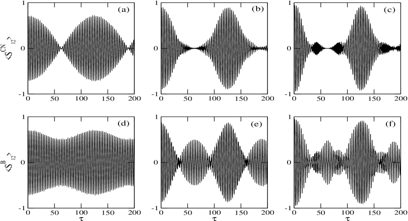
Figure 3: The top and bottom panels show the variation of average of the sine phase-difference operator $\langle S^{\rm{CN}}_{12}\rangle$ and $\langle S^{\rm{B}}_{12}\rangle$ as a function of $\tau$ for $\bar{U}=0.05$. From left to right, subplots correspond to different number of bosons $N=2$ (a,d), $N=5$ (b,e) and $N=10$ (c,f), respectively.

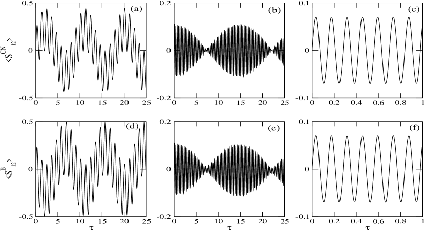
Figure 4: Same as in figure 3 but for $\bar{U}=5.0$. The subplots correspond to different number of bosons $N=2$ (a,d), $N=5$ (b,e) and $N=10$ (c,f), respectively.

3.1 A model double-well potential

A model double-well potential can be written in different forms in 1D or 2D or 3D. To study quantum phase operators for massive particles, we consider, for simplicity, a model of one-dimensional symmetric double-well potential of the form

$$V(x)=\frac{1}{2}\lambda^{2}(x^{2}-q^{2})^{2}$$ (27)

particles which has two minima at $x=\pm q$ and $\lambda$ is a parameter that determines the barrier height $V_{0}$ between the two wells given by $V_{0}=\lambda^{2}q^{4}/2$. Expanding this potential in Taylor series around $x_{\pm}=\pm q$, one finds that the leading order terms are quadratic in $(x-x_{\pm})$ and therefore small oscillations around the positions $x_{\pm}$ are simple harmonic in the leading order approximation. At the bottom of the wells around the positions $x_{\pm}$, the quantized motion of a single particle may be approximated as that of simple harmonic oscillator. Let us call the well at $x_{-}=-q$ as the left ($l$) or first (1) well and that at $x_{-}=q$ as the right ($r$) or second (2) one. In the second quantised notation, annihilation (creation) of a single-particle harmonic oscillator ground state at left (right) well can be described in terms of operators $a_{l(r)}$ ($a_{l(r)}^{\dagger}$) or equivalently $a_{1(2)}$ ($a_{1(2)}^{\dagger}$). These harmonic oscillator states of individual wells are perturbative states when the tunnelling between the wells is neglected. In the presence of tunnelling, the two lowest eigenstates of a particle in a symmetric double well potential of the form (27) are symmetric and antisymmetric combination of the two harmonic oscillator ground states which are not degenerate.

Recently, double-well potentials have become important in research with ultracold atoms in traps and optical lattices, particularly in the context of few-body quantum dynamics [18, 19], quantum tunnelling [20, 21, 22], Josephson oscillations [20], nonlinear self trapping [23, 24] correlated pair tunnelling [2, 13, 19], number squeezing [3], quantum magnetism [25] etc. Theoretical studies with interacting atoms in a double-well have demonstrated entanglement in atomic hyperfine spin and phase variables [26], an interplay between interaction and disorder in a BEC [17], operation of a quantum gate [27] and so on. With increasing use of double-wells in cold atom research, double-well optical lattice [28, 29, 30, 31] is emerging as an important tool for studying correlation effects in cold atoms [32]. Thus, addressing quantum phase problems in a toy model such as interacting particles in a symmetric double-well potential is relevant and timely in the context of current cold atom research. There are several advantages of this model. This model is generalizable for optical lattice where one can study inter-site quantum phase fluctuations and their effects on Bose-Hubbard physics [33, 34, 35, 36] and superfluid-Mott insulator quantum phase transition [35].

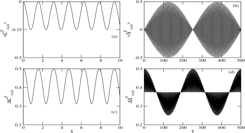
Figure 5: The subplot (a) shows the average of the fermionic cosine phase-difference operator $<C_{1u2d}>$ between the spin $\uparrow$ ($u$) in the left well (1) and the spin $\downarrow$ ($d$) in the right well (2) as a function of dimensionless time $\tau$ for $\bar{U}=0.05$. The subplot (b) shows the average of sine phase-difference operator between the same spin state. The subplots (c) and (d) display the fluctuations of the corresponding cosine and sine phase-difference operators.

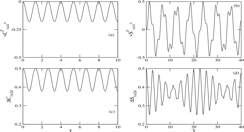
Figure 6: Same as in figure 5 but for $\bar{U}=5$.

3.2 Bosons

The Hamiltonian of a system of $N$ interacting bosons occupying two weakly coupled lowest states of a symmetric double well potential is given by

$$\hat{H}=-\hbar J(\hat{a}_{l}^{\dagger}\hat{a}_{r}+\hat{a}_{r}^{\dagger}\hat{a}_{l})+\frac{\hbar U}{2}({\hat{a}_{l}^{\dagger 2}}\hat{a}_{l}^{2}+{\hat{a}_{r}^{\dagger 2}}\hat{a}_{r}^{2})$$ (28)

where $\hat{a}_{l,r}(\hat{a}_{l,r}\dagger)$ are the bosonic particle annihilation(creation) operators for the two sites $l$ (left) and $r$ (right) of the double well, $J>0$ accounts for the hopping or tunnelling between the two sites and $U$ is the on-site interaction. The wave function $|\psi(t)\rangle$ in the basis of Fock states with fixed total particle number $N$ can be written as

$$|\psi(t)\rangle=\sum_{n_{l}=0}^{N}c_{n_{l}}(t)|n_{l},N-n_{l}\rangle$$ (29)

Where $c_{n_{l}}(t)$ is the probability amplitude to find $n_{l}$ particles in the left well and $(N-n_{l})$ particles in the right well and $|n_{l},N-n_{l}\rangle$ denote Fock state with $n_{l}$ particle at the left site and $N-n_{l}$ particle at the right site. From schrödinger equation , we obtain

$$i\frac{dc_{l}(t)}{dt}=-(\kappa_{l}c_{l+1}+\kappa_{l-1}c_{l-1})+V_{l}c_{l}$$ (30)

where $\kappa_{l}=J\sqrt{(l+1)(N-l)}$, $V_{l}=\frac{U}{2}[l^{2}+(N-l)^{2}-N]$ and the normalization condition is $\sum\limits_{l=0}^{N}|c_{l}(t)|^{2}=1$. The bosonic model we use here is similar to the one studied by Longhi [37] who has shown that the average dynamical behaviour of a pair of hard-core bosons in a symmetric double-well has a classical counterpart in the transport of electromagnetic waves through wave-guide arrays. However, such an analogy can not be drawn for fermions in general.

In the special case of $N=2$, the solution is simple and analytically tractable. For instance, let us consider the initial condition $c_{0}(0)=1$ and $c_{1}(0)=c_{2}(0)=0$ i.e. both particles are initially in the right well. One then obtains

$$c_{1}(t) = C\exp\left[-i(\frac{\bar{U}}{2}-\Omega_{\rm{B}})\tau\right]+D\exp\left[-i(\frac{\bar{U}}{2}+\Omega_{\rm{B}})\tau\right]$$

$$c_{2}(t) = c_{2}(0)+i\sqrt{2}\left[C\frac{\exp[-i(\frac{\bar{U}}{2}-\Omega_{\rm{B}})\tau]-1}{-i(\frac{\bar{U}}{2}-\Omega_{\rm{B}})}+D\frac{\exp[-i(\frac{\bar{U}}{2}+\Omega_{\rm{B}})\tau]-1}{-i(\frac{\bar{U}}{2}+\Omega_{\rm{B}})}\right]$$

$$c_{0}(t) = c_{0}(0)+i\sqrt{2}\left[C\frac{\exp[-i(\frac{\bar{U}}{2}-\Omega_{\rm{B}})\tau]-1}{-i(\frac{\bar{U}}{2}-\Omega_{\rm{B}})}+D\frac{\exp[-i(\frac{\bar{U}}{2}+\Omega_{\rm{B}})\tau]-1}{-i(\frac{U}{2}+\Omega_{B})}\right]$$

where $\bar{U}=U/J$, $\tau=Jt$, $\Omega_{\rm{B}}=\sqrt{4+(\bar{U}/2)^{2}}$, $C=\frac{(\Omega_{\rm{B}}-\frac{\bar{U}}{2})c_{1}(0)+\sqrt{2}(c_{2}(0)+c_{0}(0))}{2\Omega_{\rm{B}}}$ and $D=\frac{(\Omega_{\rm{B}}+\frac{\bar{U}}{2})c_{1}(0)-\sqrt{2}(c_{2}(0)+c_{0}(0))}{2\Omega_{\rm{B}}}$. Assuming initial condition $c_{0}(0)=1$ and $c_{1}(0)=c_{2}(0)=0$, i.e. both bosons are initially in the right well, we get $C=\frac{1}{\sqrt{2}\Omega_{\rm{B}}}$ and $D=-\frac{1}{\sqrt{2}\Omega_{\rm{B}}}$. Note that these solutions are the same as in [37].

3.3 Fermions

For many fermions in a symmetric double-well potential, it is essential to take into account a large number of single-particle states even at ultra low energy. This means that one has to consider excited states of harmonic oscillators, but then harmonic approximation of the double-well potential of (27) may break down. If one considers a few interacting two-component fermions in first two eigenstates of the harmonic oscillators around $x=\pm q$ of equation (27), one has to take into account two on-site interaction parameters - one between fermions with same spin (triplet) states and the other between dissimilar spin (singlet) states. Also, one has to consider two tunnelling terms - one between harmonic oscillator ground states and another between excited states. Thus a few fermion dynamics in a symmetric double-well potential becomes quite complicated. As an example of applications of the unitary fermion quantum phase operators, for simplicity, we assume that the kinetic energy of individual fermions is low enough so that they can occupy the low lying states of the two symmetric harmonic oscillators in the limit $\lambda\rightarrow\infty$ of the symmetric double-well potential of (27). It is assumed that the interaction between fermions is due to a contact potential. The fermion-fermion on-site interaction $U$ is assumed to be much smaller than the harmonic frequency. We then assume that the lowest harmonic oscillator states ($n=0,n^{\prime}=0$) of the two wells are occupied with all other higher states being empty. Under these conditions, for spin-polarised fermions, there are 2 possible single-particle quantum states, and for two-component fermions there are 4 single-particle quantum states corresponding to the harmonic ground states of the two sites $s=l,r$ where $s$ stands for site index. Now, if all these available low energy levels are filled up, then at low energy tunnelling dynamics of fermions may be suppressed due to Pauli blocking. For our studies we assume that quantum states are half-filled.

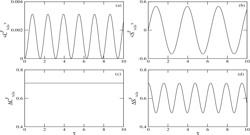
Figure 7: Same as in figure 5 but for the phase-difference operators between the spin $1\uparrow$ ($1u$) and $2\uparrow$ ($2u$).

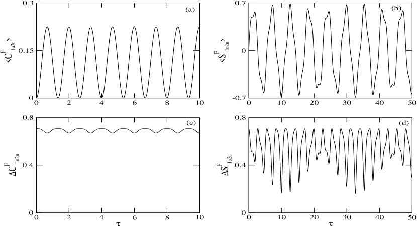
Figure 8: Same as in figure 7 but for $\bar{U}=5$

Here we deal with only two-component fermions, one with spin up and another with spin down. The Hamiltonian of the system of a pair of two-component fermions is given by

$$\hat{H} = -J\hbar(\hat{a}_{l\uparrow}^{\dagger}\hat{a}_{r\uparrow}+\hat{a}_{l\uparrow}^{\dagger}\hat{a}_{l\uparrow}+\hat{a}_{r\downarrow}^{\dagger}\hat{a}_{r\downarrow}+\hat{a}_{r\downarrow}^{\dagger}\hat{a}_{l\downarrow})$$

$$+ \frac{U\hbar}{2}(\hat{a}_{l\uparrow}^{\dagger}\hat{a}_{l\downarrow}\hat{a}_{l\downarrow}^{\dagger}\hat{a}_{l\uparrow}+\hat{a}_{r\uparrow}^{\dagger}\hat{a}_{r\downarrow}\hat{a}_{r\downarrow}^{\dagger}\hat{a}_{r\uparrow})$$

Now, we consider our trial wave function as a linear superposition of the Fock states as follows,

$$|\psi(t)\rangle = \frac{c_{1}(t)}{\sqrt{2}}(|\uparrow,\downarrow\rangle+|\downarrow,\uparrow\rangle)+c_{2}(t)|\uparrow\downarrow,0\rangle+c_{3}(t)|0,\uparrow\downarrow\rangle$$ (33)

where the states $|\uparrow,\downarrow\rangle$ , $|\downarrow,\uparrow\rangle$ define one fermion in the left well and another in right well and $|\uparrow\downarrow,0\rangle$ , $|0,\uparrow\downarrow\rangle$ define both fermions are in the left well and right well respectively. Here $c_{1}(t)$, $c_{2}(t)$ and $c_{3}(t)$ are the probability amplitudes of finding one fermion in one well, both fermions in the left and in the right well respectively. Now, putting equation $(25)$ and $(26)$ into Schrödinger equation, we get

$$i\frac{dc_{1}}{dt} = -\sqrt{2}J(c_{2}+c_{3})+\frac{U}{2}c_{1}$$

$$i\frac{dc_{2}}{dt} = -\sqrt{2}Jc_{1}+\frac{U}{2}c_{2}$$ (34)

$$i\frac{dc_{3}}{dt} = -\sqrt{2}Jc_{1}+\frac{U}{2}c_{3}$$

By solving equation $(27)$, we get

$$c_{1}(t) = A\exp\left[-i(\frac{\bar{U}}{4}-\Omega_{\rm{F}})\tau\right]+B\exp\left[-i(\frac{\bar{U}}{4}+\Omega_{\rm{F}})\tau\right]$$

$$c_{2}(t) = c_{2}(0)+i\sqrt{2}\left[A\frac{\exp[-i(\frac{\bar{U}}{4}-\Omega_{\rm{F}})\tau]-1}{-i(\frac{\bar{U}}{4}-\Omega_{\rm{F}})}+B\frac{\exp[-i(\frac{\bar{U}}{4}+\Omega_{\rm{F}})\tau]-1}{-i(\frac{\bar{U}}{4}+\Omega_{\rm{F}})}\right]$$

$$c_{3}(t) = c_{3}(0)+i\sqrt{2}\left[A\frac{\exp[-i(\frac{\bar{U}}{4}-\Omega_{\rm{F}})\tau]-1}{-i(\frac{\bar{U}}{4}-\Omega_{\rm{F}})}+B\frac{\exp[-i(\frac{\bar{U}}{4}+\Omega_{\rm{F}})\tau]-1}{-i(\frac{U}{4}+\Omega_{F})}\right]$$

where $\Omega_{\rm{F}}=\sqrt{4+(\frac{\bar{U}}{4})^{2}}$, $A=\frac{(\Omega_{\rm{F}}-\frac{\bar{U}}{4})c_{1}(0)+\sqrt{2}(c_{2}(0)+c_{3}(0))}{2\Omega_{\rm{F}}}$ and $B=\frac{(\Omega_{\rm{F}}+\frac{\bar{U}}{4})c_{1}(0)-\sqrt{2}(c_{2}(0)+c_{3}(0))}{2\Omega_{\rm{F}}}$. Assuming initial condition $c_{3}(0)=1$ and $c_{1}(0)=c_{2}(0)=0$, i.e. both fermions are initially in the right well, we get $A=\frac{1}{\sqrt{2}\Omega_{\rm{F}}}$ and $B=-\frac{1}{\sqrt{2}\Omega_{\rm{F}}}$.

4 Results and discussions

We first present results on averages of phase-difference operators for bosons. We assume that bosons are initially in the right well. In figure 1 we show the average of the non-unitary Carruther-Nieto cosine phase-difference operators and compare it with that of our unitary cosine phase-difference operators for 3 different numbers of total bosons for the interaction strength $\bar{U}=0.05$. Figure 2 shows the same as in figure 1 but for $\bar{U}=5$. Comparing the plots in figure 1 with those in figure 2 we notice that the average of the unitary cosine phase-difference operators deviate largely from that of the non-unitary ones particularly in the low energy regime. Figures 3 and 4 display variation of the average of the non-unitary and unitary sine phase-difference operators for $\bar{U}=0.5$ $\bar{U}=5$, respectively, for different number of bosons. A comparison between the figures 3 and 4 shows that for large number of bosons and at large interaction strength, the averages of unitary and non-unitary sine phase-difference operators are almost similar. In terms of absolute magnitude and gross dynamical features, the deviations of the results for non-unitary sine phase-difference operators from those for unitary ones seem to be not as large as in the case of cosine phase-difference operators.

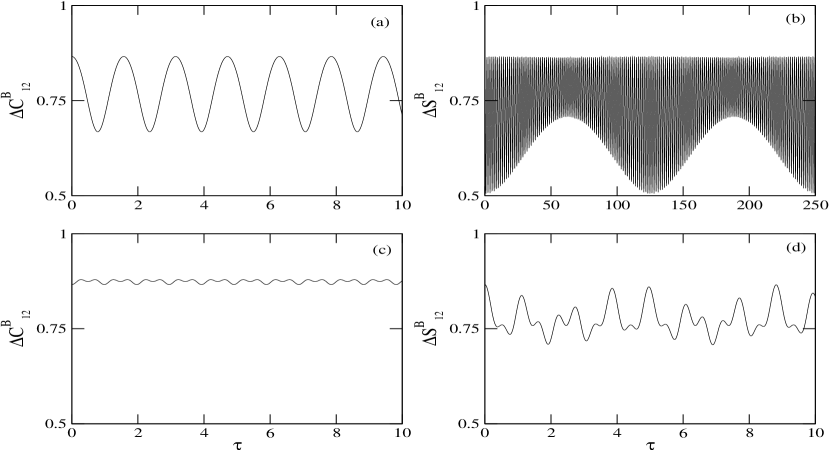
Figure 9: Fulctuations in cosine (a and c) and sine (b and d) phase-difference operators for a pair of bosons are plotted as a function of $\tau$ for $\bar{U}=0.05$ (a, b) and $\bar{U}=5$ (c and d)

.

Using the analytical expression of equations (31) we find that for two bosons and $\bar{U}=0$, $\langle C^{CN}_{12}\rangle=0$ $\langle S^{CN}_{12}\rangle=\frac{1}{\sqrt{2}}\sin(2\tau)$, $\langle C^{B}_{12}\rangle=\frac{1}{8}(\cos(4\tau)-1)$, and $\langle S^{B}_{12}\rangle=\frac{1}{\sqrt{2}}\sin(2\tau)$. For small $\bar{U}$, the interference between two time scale shows features like collapses and revivals in average quantities. For $\bar{U}\gg 0$, the quantum mechanical average of $C^{CN}_{12}$, $S^{CN}_{12}$ and $C^{B}_{12}$, $S^{B}_{12}$ tend to be identical. For bosons larger than 2, we find when $\bar{U}=0$, $\langle C^{CN}_{12}\rangle=0$ and $\langle S^{CN}_{12}\rangle\neq 0$ for any number of bosons but both terms are nonzero for $\bar{U}\neq 0$. When $\bar{U}=0$ it is found that $\langle C^{B}_{12}\rangle=0$ for odd number number of bosons and $\langle C^{B}_{12}\rangle\neq 0$ for even number of bosons. For large number of bosons unitary and non-unitary phase difference operators provide almost the same results. In short, unitary phase-difference operators are important for low number of bosons.

To study phase properties of fermions, we consider two-mode fermion phase-difference operators of equations (24) and (25) of a pair of two-component fermions. We can enumerate mainly 3 pairs of modes which are (a) $m\equiv l\uparrow$ and $m^{\prime}\equiv r\uparrow$; (b) $m\equiv l\uparrow$ and $m^{\prime}\equiv r\downarrow$ (or $m\equiv l\downarrow$ and $m^{\prime}\equiv r\uparrow$); (c) $m\equiv l\downarrow$ and $m^{\prime}\equiv r\downarrow$; where $r$ and $l$ implies right and left well harmonic oscillator ground states. For the mode-pair (a) there are two configurations for state like $\mid 10\rangle_{i}$ yielding $\sum_{i}\mid 10\rangle_{i}=\mid\uparrow\downarrow,0\rangle+\mid\uparrow,\downarrow\rangle$. In the case of mode-pair (b), the number of configurations in which up spin on the left well is occupied while down spin on the right well is empty is only one. Therefore in the case (b), we have $\sum_{i}\mid 10\rangle_{i}=\mid\uparrow\downarrow,0\rangle$. We study quantum phase-difference for the cases (a) and (b) only.

Figures 5 demonstrates average and fluctuations of fermionic phase-difference operators between the two modes $1\uparrow$ and $2\downarrow$ for $\bar{U}=0.05$ while figure 6 exhibits the same for $\bar{U}=5$. From these two figures we notice that both the average and fluctuation of cosine phase-difference operator exhibit sinusoidal behaviour as a function of time while those of sine phase-difference operators show collapse and revivals depending on the interaction strengths. Figure 7 displays the results for average and fluctuation of fermionic phase-difference operators for spin $\uparrow$ in both the wells for $\bar{U}=0.05$. Figure 8 is the counterpart of figure 7 for $\bar{U}=5$. We infer from figure 7 and 8 that for low $\bar{U}$, both the average and fluctuation quantities show almost sinusoidal variation as a function of time. Comparing the figure 7 with figure 5, we notice that phase fluctuations in both cosine and sine phase-difference operators at low $\bar{U}$ is larger in case of two same spin states compared to that in case of two different spin states. To compare phase fluctuations of a pair of two-component fermions with those of a pair of single-component b bosons, we display the dynamical evolution of he fluctuations in cosine and sine phase-difference operators for a pair of bosons in figure 9. Comparing figure 9 with figure 5 we notice that quantum phase fluctuation characteristics of pair of indistinguishable bosons in a 1D symmetric double-well potential are qualitatively different from those of a pair of two-component fermions under similar physical condition, although averages of quantum phases in the two case may be qualitatively similar as can be inferred from a comparison between figure 3(a) and figure 5(b). Note that for the 1D model considered here, the results for a pair of two-component fermions will be expected to be the same as that of a pair of two-component bosons. However, two-component many-fermion case in higher dimensions would exhibit quantum phase properties different from that of two-component bosons.

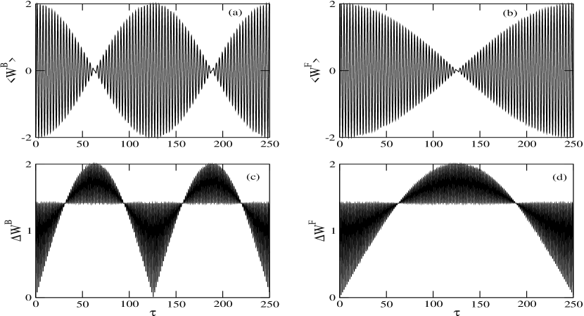
Figure 10: Shown are the plots of the average of number-difference operators for a pair of bosons (a) and a pair of two-component fermions (b) for $\bar{U}=0.5$. The subplots (c) and (d) exhibit the fluctuations of the corresponding number-difference operators

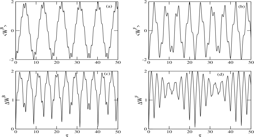
Figure 11: Same as in figure 10 but for $\bar{U}=5$.

We now present results on average and fluctuations of number-difference operators for a pair of bosons and a pair of two-component fermions in figures 10 and 11. Note that the number-difference fluctuation $\Delta\hat{W}^{\rm{B}}_{12}$ is closely related to the the two-mode squeezing parameter which in turn describes entanglement between two bosonic modes in terms of number variables. Since quantum phase-difference operators are canonically conjugate to number-difference operators, two-mode number squeezing (reduced fluctuations in number-difference operators) would be related to enhanced fluctuations in quantum phase-difference operators. In other words, two-mode quantum phase fluctuations are also related to the two-mode entanglement. The entanglement between the two modes in number variables can be quantified as the two-mode squeezing [38] or entanglement [39, 40] parameter given by

$$\xi_{n}=(\Delta(\hat{n}_{l}-\hat{n}_{r}))^{2}/(\langle\hat{n}_{l}\rangle+\langle\hat{n}_{r}\rangle)=\frac{\left(\Delta\hat{W}^{\rm{B}}_{12}\right)^{2}}{N}$$ (36)

The two modes become entangled when $\xi_{n}$ is less than unity, or equivalently, when $\sqrt{\Delta\hat{W}^{\rm{B}}}$ becomes less than $\sqrt{N}$. The entanglement parameter $\xi^{F}_{n}$ for two-component fermions in terms of total fermion number fluctuation is given by

$$\xi^{\rm{F}}_{n}=2\left[1-\frac{2}{\Omega_{\rm{F}}^{2}}\sin^{2}(\Omega_{\rm{F}}\tau)-\frac{1}{4\Omega_{\rm{F}}^{2}}[\Omega_{\rm{F}}^{-}\cos(\Omega_{\rm{F}}^{+}\tau)-\Omega_{\rm{F}}^{+}\cos(\Omega_{\rm{F}}^{-}\tau)]^{2}\right]$$ (37)

where $\Omega_{\rm{F}}^{-}=\Omega_{\rm{F}}-\bar{U}/4$, $\Omega_{\rm{F}}^{+}=\Omega_{\rm{F}}+\bar{U}/4$. From the expression (37) it is clear that $\xi^{\rm{F}}_{n}$ can oscillate between 0 and 2. Figure 10 (c) shows that when the interaction is small ($\bar{U}=0.05$), there are time domains where the number-difference fluctuation remains bounded between 0 and $\sqrt{2}$ and so the two bosons can be said to be entangled in those time domains. The same is also true for fermions (figure 10 (d)). Subplots 10(a) and 10(b) exhibit that there are trapping states both for bosons and fermions when the average of number-difference operators vanish. We notice that near such trapping states the number-difference fluctuations are greater than $\sqrt{2}$ and hence when trapping occurs the two wells are not entangled in number variables. The time domains where entanglement occurs are far from trapping times where the average of number-difference oscillates largely. Figure 10 shows that for large $U$ trapping does not occur and there is no time domain for entanglement. Comparing figure 10(d) with figure 5(d), we infer that the reduced fluctuation in fermionic number-difference operator with enhanced fluctuation in sine phase-difference operator or vice-versa occur at the same time domain. This illustrates number-phase uncertainty in fermionic systems in terms of unitary quantum phase operators.

5 Conclusions

In conclusion we have introduced Hermitian and unitary two-mode quantum phase-difference operators for bosons and fermions. Our results reveal the importance of unitary phase-operators in describing quantum phase properties of a few bosons or fermions. To the best of our knowledge, the problem of unitary quantum phase operators for matter waves has been addressed for the first time in this work. Our model studies on the comparison between non-unitary and unitary bosonic phase operators reveal that the results for unitary phase operators are substantially different from those for non-unitary ones particularly in the case of a low number of bosons. In our quantum phase formalism, the unitarity of phase operators is ensured by coupling vacuum state of one mode of matter waves with the highest number state of the same mode in a finite dimensional Fock space. In case of a Bose-Einstein condensate (BEC) in a double-well potential, non-unitary phase operators [17] are used in theoretical studies of quantum phases between the two BEC’s in two wells. In case of large number of particles as in a BEC, due to statistical effects unitary and non-unitary quantum phase operators are expected to yield similar results because vacuum fluctuations in case of a macroscopically large number of particles may not play a dominant role. However, a few bosons in a double-well potential is truly a quantum system where vacuum fluctuations can not be neglected and hence unitary quantum phase operators are essential for measuring quantum phases of a few-body quantum system.

Using the quantum phase operators we have studied in detail the effects of on-site interaction on quantum phase and number fluctuation properties of interacting bosons and a pair two-component interacting fermions in a 1D symmetric double-well potential as an example. In terms of number variables, both bosonic and fermionic systems exhibit interesting inter-well entanglement properties which may be a potential resource for future quantum information processing with neutral atoms in double-well optical lattices. It would be interesting to explore entanglement properties of a few-body quantum system in terms of these newly introduced unitary quantum phase operators. With the first demonstration of homo-dyne detection of a fluctuating continuous variable of matter waves by Gross et al. [41] in 2011, it might be possible in near future to perform experiments on the measurement of quantum phases of matter waves in a similar manner as in Mandel’s experiments that require homo-dyne or hetero-dyne detection of weak signals. The fermionic phase operators introduced here are applicable for a many-fermion system that has to be treated within a framework of configuration-interaction or other many-body formalism which requires a separate study.

6 Acknowledgment

Biswajit Das is thankful to the Council of Scientific & Industrial Research (CSIR), Govt. of India, for a support.

* Present address: Bhaba Atomic Research Centre, Mumbai 400085, INDIA.

References

References

- [1] Shin Y, Saba M, Pasquini T A, Ketterle W, Pritchard D E and Leanhardt A E 2004 Phys. Rev. Lett. 92 050405
- [2] Fölling S, Trotzky S, Cheinet P C, Feld M, Saers R, Widera A, Mueller T and Bloch I 2007 Nature 448 1029
- [3] Sebby-Strabley J , Brown B L, Anderlini M, Lee P J, Phillips W D and Porto J V 2007 Phys. Rev. Lett. 98 200405
- [4] Dirac P A M 1927 Proc. R. Soc. A 114 243
- [5] Louisell W H 1963 Phys. Lett. 7 60
- [6] Susskind L and Glogower J 1964 Physics 1 49-61
- [7] Carruthers P, Nieto M M 1968 Rev. Mod. Phys. 40 2
- [8] Barnett S M and Pegg D T 1986 J. Phys. A 19 3849
- [9] Noh J W, Fougeres A and Mandel L 1991 Phys. Rev. Lett. 67 11
- [10] Noh J W, Fougeres A and Mandel L 1992 Phys. Rev. A 45 1
- [11] Noh J W, Fougeres A and Mandel L 1993 Phys. Rev. Lett. 71 16
- [12] Noh J W, Fougeres A and Mandel L 1994 Phys. Rev. A 49 1
- [13] Chen Y-A, Nascimbène, Aidelsburger S M, Atala M, Trotzky S, Bloch I. 2011 Phys. Rev. Lett. 107 210405
- [14] Deb B, Gangopadhyay G and Ray D S 1993 Phys. Rev. A 48 2
- [15] Deb B 1996 Ph. D. thesis (unpublished) Jadavpur University Kolkata, India.
- [16] Peřinova V, Lukš A and Peřina J 1998 “Phase in Optics”( World Scietific Series in Contemporary Chemical Physics; vol. 15) (Singapore: World Scientific Publishing co. Pte. Ltd.)
- [17] Zhou Q and Sarma S D 2010 Phys. Rev. A 82 041601 (R)
- [18] Zollner S, Meyer H-D and Schmelcher P 2008 Phys. Rev. A 78 013621
- [19] Zollner S, Meyer H-D and Schmelcher P 2008 Phys. Rev. Lett. 100 040401
- [20] Albiez M et al. 2005 Phys. Rev. Lett. 95 010402
- [21] Milburn G J, Corney J, Wright E M and Walls D F 1997 Phys. Rev. A 55 4318
- [22] Kierig E, Schnorrberger U, Schietinger A, Tomkovic J and Oberthaler M K 2008 Phys. Rev. Lett. 100 190405
- [23] Anker T et al. 2005 Phys. Rev. Lett. 94 020403
- [24] Javanainen J 1986 Phys. Rev. Lett. 57 3164
- [25] Trotzky S et al. 2008 Science 319 295-299
- [26] Barmettler P, Rey A-M, Demler E, Lukin M D, Bloch I, Gritsev V 2008 Phys. Rev. A 78 012330
- [27] Foot C J, Shotter M D 2011 Am. J. Phys 79 7
- [28] Anderlini M, Sebby-Strabley J, Kruse J, Porto J V and Phillips W D 2006 J. Phys. B : At. Mol. Opt. Phys 39 S199-S210
- [29] Sebby-Strabley J, Anderlini M, Jessen P S and Porto J V 2006 Phys. Rev. A 73 033605
- [30] Stojanovic V M, Wu C, Liu V and Sarma S D 2008 Phys. Rev. Lett. 101 125301
- [31] Lee P J, Anderlini M, Brown B L, Sebby-Strabley J, Phillips W D and Porto J V 2007 Phys. Rev. Lett. 99 020402
- [32] Anderlini M et al. 2007 Nature 448 452-456
- [33] Fisher M P A, Weichman P B, Grinstein G and Fisher D S 1989 Phys. Rev. B 40 546
- [34] Sheshadri K, Krishnamurthy H R, Pandit R and Ramakrishnan T V 1993 Europhys. Lett. 22 257-263
- [35] Greiner M, Mandel O, Esslinger T, Hansch T W and Bloch I 2002 Nature 415 39-44
- [36] Jaksch D, Breigel H, Cirac J, Gardiner C and Zoller P 1999 Phys. Rev. Lett. 82 1975
- [37] Longhi S 2011 J. Phys. B : At. Mol. Opt. Phys 44 051001
- [38] Barnett S M and Radmore P M 1997 “Methods in Theoretical Quantum Optics” Oxford University Press
- [39] Gasenzer T, Roberts D C and Burnett K 2002 Phys. Rev. A 65 021605 (R)
- [40] Deb B, Agarwal G S 2002 Phys. Rev. A 65 063618
- [41] Gross C et al. 2011 Nature 480 219-223