Abstract

Embryonic development is driven by spatial patterns of gene expression that determine the fate of each cell in the embryo. While gene expression is often highly erratic, embryonic development is usually exceedingly precise. In particular, gene expression boundaries are robust not only against intra-embryonic fluctuations such as noise in gene expression and protein diffusion, but also against embryo-to-embryo variations in the morphogen gradients, which provide positional information to the differentiating cells. How development is robust against intra- and inter-embryonic variations is not understood. A common motif in the gene regulation networks that control embryonic development is mutual repression between pairs of genes. To assess the role of mutual repression in the robust formation of gene expression patterns, we have performed large-scale stochastic simulations of a minimal model of two mutually repressing gap genes in Drosophila, hunchback (hb) and knirps (kni). Our model includes not only mutual repression between hb and kni, but also the stochastic and cooperative activation of hb by the anterior morphogen Bicoid (Bcd) and of kni by the posterior morphogen Caudal (Cad), as well as the diffusion of Hb and Kni between neighboring nuclei. Our analysis reveals that mutual repression can markedly increase the steepness and precision of the gap gene expression boundaries. In contrast to other mechanisms such as spatial averaging and cooperative gene activation, mutual repression thus allows for gene-expression boundaries that are both steep and precise. Moreover, mutual repression dramatically enhances their robustness against embryo-to-embryo variations in the morphogen levels. Finally, our simulations reveal that diffusion of the gap proteins plays a critical role not only in reducing the width of the gap gene expression boundaries via the mechanism of spatial averaging, but also in repairing patterning errors that could arise because of the bistability induced by mutual repression.

Introduction

The development of multicellular organisms requires spatially controlled cell differentiation. The positional information for the differentiating cells is typically provided by spatial concentration gradients of morphogen proteins. In the classical picture of morphogen-directed patterning, cells translate the morphogen concentration into spatial gene-expression domains via simple threshold-dependent readouts [1, 2, 3, 4]. Yet, while embryonic development is exceedingly precise, this mechanism is not very robust against intra- and inter-embryonic variations [5, 6, 7]: the spatial patterns of the target genes do not scale with the size of the embryo and the boundaries of the expression domains are susceptible to fluctuations in the morphogen levels and to the noise in gene expression. Intriguingly, the target genes of morphogens often mutually repress each other, as in the gap-gene system of the fruit fly Drosophila [8, 9, 10, 11, 12, 13, 14]. To elucidate the role of mutual repression in the robust formation of gene expression patterns, we have performed extensive spatially-resolved stochastic simulations of the gap-gene system of Drosophila melanogaster. Our results show that mutual repression between target genes can markedly enhance both the steepness and the precision of gene-expression boundaries. Furthermore, it makes them robust against embryo-to-embryo variations in the morphogen gradients.

The fruit fly Drosophila melanogaster is arguably the paradigm of morphogenesis. During the first 90 minutes after fertilization it is a syncytium, consisting of a cytoplasm that contains rapidly diving nuclei, which are not yet encapsulated by cellular membranes. Around cell cycle 10 the nuclei migrate towards the cortex of the embryo and settle there to read out the concentration gradient of the morphogen protein Bicoid (Bcd), which forms from the anterior pole after fertilization [3]. One of the target genes of Bcd is the gap gene hunchback (hb), which is expressed in the anterior half of the embryo. In spite of noise in gene expression, the midembryo boundary of the hb expression domain is astonishingly sharp. By cell cycle 11, the hb mRNA boundary varies by about one nuclear spacing only [15, 16, 17], while by cell cycle 13 a similarly sharp oundary is observed for the protein level [5, 6, 18]. This precision is higher than the best achievable precision for a time-averaging based readout mechanism of the Bcd gradient [6]. Interestingly, the study of Gregor et al. revealed that the Hb concentrations in neighboring nuclei exhibit correlations and the authors suggested that this implies a form of spatial averaging that enhances the precision of the posterior Hb boundary [6]. Two recent simulation studies suggest that the mechanism of spatial averaging is based on the diffusion of Hb itself [19, 20]; as shown analytically in [19], Hb diffusion between neighboring nuclei reduces the super-Poissonian part of the noise in its concentration. In essence, diffusion reduces noise by washing out bursts in gene expression. However, the mechanism of spatial averaging comes at a cost: it tends to lessen the steepness of the expression boundaries.

Bcd induces the expression of not only hb, but a number of gap genes, and pairs of gap genes tend to repress each other mutually. Interestingly, repression between directly neighboring gap genes is weak, whereas repression between non-adjacent genes is strong [21]. hb forms a strongly repressive pair with knirps (kni) which is expressed further towards the posterior pole; both genes play a prominent role in the later positioning of downstream pair-rule gene stripes [9]. It has been argued that mutual repression can enhance robustness to embryo-to-embryo variations in morphogen levels [12, 13, 14] and sharpen a morphogen-induced transition between the two mutually repressing genes in a non-stochastic background [22, 23]. However, mutual repression can also lead to bistability [24, 25, 26, 27, 28]. While bistablity may buffer against inter-embryo variations and rapid intra-embryo fluctuations in morphogen levels, it may also cause stochastic switching between distinct gene expression patterns, which would be highly detrimental. Therefore, the precise role of mutual repression in the robust formation of gene-expression patterns remains to be elucidated.

While the role of antagonistic interactions in the formation of gene-expression patterns has been studied using mean-field models [12, 28, 29, 30, 31], to address the question whether mutual repression enhances the robustness of these patterns against noise arising from the inherent stochasticity of biochemical reactions a stochastic model is essential. We have therefore performed large-scale stochastic simulations of a minimal model of mutual repression between hb and kni. Our model includes the stochastic and cooperative activation of hb by Bcd and of kni by the posterior morphogen Caudal (Cad) [32, 33]. Moreover, Hb and Kni can diffuse between neighboring nuclei and repress each other’s expression, generating two separate spatial domains interacting at midembryo (see Fig. 1). We analyze the stability of these domains by systematically varying the diffusion constants of the Hb and Kni proteins, the strength of mutual repression and the Bcd and Cad activator levels. To quantify the importance of mutual repression, we compare the results to those of a system containing only a single gap gene, which is regulated by its morphogen only; this is the “system without mutual repression”. While our model is simplified—it neglects, e.g., the interactions of hb and kni with krüppel (kr) and giant (gt) [34]—it does allow us to elucidate the mechanism by which mutual repression can enhance the robust formation of gene expression patterns.

One of the key findings of our analysis is that mutual repression enhances the robustness of the gene expression domains against intra-embryonic fluctuations arising from the intrinsic stochasticity of biochemical reactions. Specifically, mutual repression increases the precision of gene-expression boundaries: it reduces the variation $\Delta x$ in their positions due to these fluctuations. At the same time, mutual repression also enhances the steepness of the expression boundaries. To understand the interplay between steepness, precision and intra-embryonic fluctuations (biochemical noise), it is instructive to recall that the width $\Delta x$ of a boundary of the expression domain of a gene $g$ is, to first order, given by

$$\Delta x=\frac{\sigma_{\mathrm{G}}(x_{\mathrm{t}})}{|\langle G(x_{\mathrm{t}})\rangle^{\prime}|},$$ (1)

where $\sigma_{\mathrm{G}}(x_{\mathrm{t}})$ is the standard deviation of the copy number $G$ of protein G and $|\langle G(x_{\mathrm{t}})\rangle^{\prime}|$ is the magnitude of the gradient of $G$ at the boundary position $x_{\mathrm{t}}$ [6, 35, 19]. Steepness thus refers to the slope of the average concentration profile, $|\langle G(x_{\mathrm{t}})\rangle^{\prime}|$, while precision refers to $\Delta x$, which is the standard deviation in the position at which $G$ crosses a specified threshold value, here taken to be the half-maximal average expression level of $G$.

The simulations reveal, perhaps surprisingly, that mutual repression hardly affects the noise $\sigma_{\mathrm{G}}(x_{\mathrm{t}})$ at the expression boundaries of hb and kni. Moreover, mutual repression can strongly enhance the steepness $|\langle G(x_{\mathrm{t}})\rangle^{\prime}|$ of these boundaries: the steepness of the boundaries in a system with mutual repression can, depending on the diffusion constant, be twice as large as that in the system without mutual repression. Together with Eq. 1, these observations predict that mutual repression can significantly enhance the precision of the boundaries, i.e. decrease $\Delta x$, which is indeed precisely what the simulations reveal. Interestingly, there exists an optimal diffusion constant that minimizes the boundary width $\Delta x$, as has been observed for a system without mutual repression [19]. While the minimal $\Delta x$ of the system with mutual repression is only marginally lower than that of the system without it, this optimum is reached at a lower value of the diffusion constant, where the steepness of the boundaries is much higher. We find that these observations are robust, i.e. independent of the precise parameters of the model, such as maximum expression level, size of the bursts of gene expression, and the cooperativity of gene activation.

Our results also show that mutual repression can strongly buffer against embryo-to-embryo variations in the morphogen levels by suppressing boundary shifts via a mechanism that is akin to that of [36, 37]. A more detailed analysis reveals that when the regions where Bcd and Cad activate hb and kni respectively overlap, bistability can arise in the overlap zone. Yet, the mean waiting time for switching is longer than the lifetime of the morphogen gradients, which means that the hb and kni expression patterns are stable on the relevant developmental time scales. This also means, however, that when errors are formed during development, these cannot be repaired. Here, our simulations reveal another important role for diffusion: without diffusion a spotty phenotype emerges in which the nuclei in the overlap zone randomly express either Hb or Kni; diffusion can anneal these patterning defects, leading to well-defined expression domains of Hb and Kni. Finally, we also study a scenario where hb and kni are activated by Bcd only. While this scheme is not robust against embryo-to-embryo variations in the morphogen levels, mutual repression does enhance boundary precision and steepness also in this scenario.

Results

Model

We consider the embryo in the syncytial blastoderm stage at late cell cycle 14, ca. $2~{}\,\mathrm{h}$ after fertilization. In this stage the majority of the nuclei forms a cortical layer and hb and kni expression can be detected [11]. Our model is an extension of the one presented in [19]. It is based on a cylindrical array of diffusively coupled reaction volumes which represent the nuclei, with periodic boundary conditions in the angular ($\phi$) and reflecting boundaries in the axial ($x$) direction. The dimensions of the cortical array are $N_{\mathrm{x}}=N_{\mathrm{\phi}}=64$, with equal spacing of the nuclei $\ell=8.5\,\mathrm{\mu m}$ in both directions. For a given embryo length $L$, this implies a cylinder radius $R=\frac{L}{2\pi}\simeq\frac{L}{6}$, which is close to the experimentally observed ratio. The resulting number of $N=4096$ nuclei roughly corresponds to the expected number of cortical nuclei at cell cycle 14 if non-dividing polyploid yolk nuclei are taken into account [38] (see Text S1 for details); we also emphasize, however, that none of the results presented below depend on the precise number of nuclei.

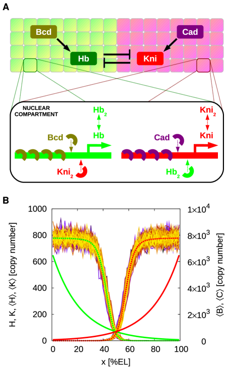
Figure 1: The model. (A) Cartoon of our model. Bcd activates hb, while its antagonist kni is activated by Cad. The gap genes hb and kni repress each other mutually. In each nuclear compartment we simulate the genetic promoters of both hb and kni. Activation is cooperative: In the default setting, 5 morphogen proteins have to bind to the promoter to initiate gene expression. Hb and Kni both form homodimers, which can bind to the other gene’s promoter to totally block expression, irrespective of the number of bound morphogen proteins. Both dimers and monomers travel between neighboring nuclear compartments via diffusion. (B) Protein copy number profiles along the AP axis in a typical simulation in steady state, with parameter values as in Table S2 in Text S1. Plotted are the morphogen gradients Bcd ($\langle B\rangle$, solid green line) and Cad ($\langle C\rangle$, solid red line) and the resulting Hb ($H$) and Kni ($K$) total copy number profiles for different times. The dashed green and red lines show the Hb ($\langle H\rangle$) and Kni ($\langle K\rangle$) profiles averaged over time and the circumference of the (cylindrical) system.

In each nuclear volume we simulate the activation of the gap genes hb and kni by the morphogens Bcd and Cad, respectively, and mutual repression between hb and kni (see Fig. 1). In what follows, we will refer to Hb and Kni as repressors and to Bcd and Cad as activators. Our model of gene regulation bears similarities to those of [39, 40, 30, 31, 28], in the sense that it is based on a statistical mechanical model of gene regulation by transcription factors, allowing the computation of promoter-site occupancies. However, the models of [39, 40, 30, 31, 28] are mean-field models, which cannot capture the effect of intra-embryonic fluctuations due to biochemical noise arising from the inherent stochasticity of biochemical reactions. This requires a stochastic model; moreover, it necessitates a model in which the transitions between the promoter states are taken into account explicitly, since these transitions form a major source of noise in gene expression, as we will show. To limit the number of combinatorial promoter states, we have therefore studied a minimal model that only includes Bcd, Cad, Hb and Kni. Following [19], we assume that Bcd and Cad bind stochastically and cooperatively to $n_{\mathrm{max}}$ sites on their target promoters. To obtain a lower bound on the precision of the hb and kni expression domains, we assume that the activating morphogens Bcd and Cad bind to their promoters with a diffusion-limited rate $k_{\mathrm{\rm on}}^{\rm A}=4\pi\alpha D_{\mathrm{A}}/V$, where $\alpha$ is the dimension of a binding site, $D_{\mathrm{A}}$ is the diffusion constant of the morphogen, and $V$ is the nuclear volume (see “Materials & Methods” for parameter values). Since the morphogen-promoter association rate is assumed to be diffusion limited, cooperativity of hb and kni activation is tuned via the dissociation rate $k_{\mathrm{\rm off,n}}^{\rm A}=a/b^{n}$, which decreases with increasing number $n$ of promoter-bound morphogen molecules. The baseline parameters are set such that the half-maximal activation level of hb and kni is at midembryo, and the effective Hill coefficient for gene activation is around 5 [19]; while we will vary the Hill coefficient, this is our baseline parameter. Again to obtain a lower bound on the precision of the gap-gene expression boundaries, transcription and translation is concatenated in a single step. Mutual repression between hb and kni occurs via binding of Hb to the kni promoter, which blocks the expression of kni irrespective of the number of bound Cad molecules, and vice versa. To assess the importance of bistability, Hb and Kni can homodimerize and bind to their target promoters only in their dimeric form, which is a prerequisite for bistability in the mean-field limit [24]. Both the monomers and dimers diffuse between neighboring nuclei and are also degraded; the effective degradation rate $\mu_{\mathrm{\rm eff}}$ is such that the gap-gene expression domains can form sufficiently rapidly on the time scale of embryonic development ($\approx 10-20~{}\,\mathrm{min}$ [38]). In the absence of mutual repression, our model behaves very similarly to that of [19], even though our model contains both monomers and dimers instead of only monomers.

Motivated by experiment [3, 5, 7], and in accordance with the diffusion-degradation model, we adopt an exponential shape for the stationary Bcd profile; we thus do not model the establishment of the gradient [41]. To elucidate the role of mutual repression, it will prove useful to take our model to be symmetric: the Cad profile is the mirror image of the Bcd profile, and hb and kni repress each other equally strongly. Diffusion of Bcd and Cad between nuclei induce fluctuations in their copy numbers on the time scale $\tau_{\mathrm{d}}=\ell^{2}/(4D_{\mathrm{A}})\simeq 6~{}\,\mathrm{s}$. Because $\tau_{\mathrm{d}}$ is much smaller than the time scale for promoter binding, $1/k_{\mathrm{\rm on}}^{\rm A}\simeq 360~{}\,\mathrm{s}$, fluctuations in the copy number of Bcd and Cad are effectively averaged out by slow binding of Bcd and Cad to their respective promoters, hb and kni [19]. To elucidate the importance of the threshold positions for hb and kni activation, we will scale the morphogen gradients by a global dosage factor $A$; this procedure will also allow us to study the robustness of the system against embryo-to-embryo variations in the morphogen levels.

We simulate the model using the Stochastic Simulation Algorithm (SSA) of Gillespie [42, 43]. Diffusion is implemented into the scheme via the next-subvolume method used in MesoRD [44, 45]. A recent version of our code is available at GitHub and can be accessed via http://ggg.amolf.nl .

Characteristics of gap-gene expression boundaries

Three key characteristics of gene expression boundaries are 1) the noise in the protein concentration at the boundary; 2) the steepness of the boundary; 3) the width of the boundary. While these quantities may make intuitive sense, their definitions are not unambiguous. Equally important, different definitions will reveal different properties of the system.

Decomposing the noise. Let’s consider the variance in the copy number $G$ of protein G at position $x$ along the anterior-posterior (AP) axis. We define its mean copy number, averaged over all embryos, circumferential positions $\phi$ and all times, at the anterior-posterior position $x$ as

$$\overline{\langle\langle{G}\rangle_{\phi}\rangle_{e}}(x) \equiv \frac{1}{N_{\mathrm{e}}}\frac{1}{T}\frac{1}{N_{\mathrm{\phi}}}\sum_{\mathrm{e=0}}^{N_{\mathrm{e}}-1}\sum_{\mathrm{t=0}}^{T-1}\sum_{\mathrm{\phi=0}}^{N_{\mathrm{\phi}}-1}G_{\mathrm{e}}(\phi,x,t),$$ (2)

where $G_{\mathrm{e}}(x,\phi,t)$ is the copy number of protein G in embryo $e$ at position $x$ and angle $\phi$ in the circumferential direction (perpendicular to the AP-axis) at time $t$. Here, we introduce the convention that the overline denotes an average in time, while the ensemble brackets with a subscript $\phi$ denote an average along the $\phi$ direction and that with a subscript $e$ an average over all embryos. The variance in the copy number $G\equiv G_{\mathrm{e}}(x,\phi,t)$ is then given by

$$\sigma^{2}_{\mathrm{G}}(x) = \overline{\langle\langle{(G-\overline{\langle\langle{G}\rangle_{\phi}\rangle_{e}})^{2}}\rangle_{\phi}\rangle_{e}}$$ (3)

$$= \langle\overline{\langle{G^{2}}\rangle_{\phi}}\rangle_{\mathrm{e}}-\langle\overline{\langle G\rangle_{\mathrm{\phi}}^{2}}\rangle_{\mathrm{e}}+\langle\overline{\langle G\rangle_{\mathrm{\phi}}^{2}}\rangle_{\mathrm{e}}-\langle\overline{\langle{G}\rangle_{\phi}}^{2}\rangle_{\mathrm{e}}+\langle\overline{\langle{G}\rangle_{\phi}}^{2}\rangle_{\mathrm{e}}-\overline{\langle\langle{G}\rangle_{\phi}\rangle_{e}}^{2}$$ (4)

$$= \overbrace{\langle\overline{\sigma^{2}_{\mathrm{G}}}\rangle_{\mathrm{e}}(x)+\langle\sigma^{2}_{\mathrm{\langle G\rangle_{\mathrm{\phi}}}}\rangle_{\mathrm{e}}(x)}^{\text{mean intra-embryonic noise}}\hskip 78.52945pt+\overbrace{\sigma^{2}_{\mathrm{\langle\overline{G}\rangle_{\mathrm{\phi}}}}(x)}^{\text{inter-embryonic variations}}$$ (5)

The total variance in the copy number can thus be decomposed into intra-embryonic fluctuations averaged over all embryos and inter-embryonic variations. The former can, furthermore, be decomposed into $\langle\overline{\sigma^{2}_{\mathrm{G}}}\rangle_{\mathrm{e}}(x)$, which is the time-averaged mean of the variance in $G$ along the circumferential direction, $\overline{\sigma^{2}_{\mathrm{G}}}(x)$, averaged over all embryos, and $\langle\sigma^{2}_{\mathrm{\langle G\rangle_{\mathrm{\phi}}}}\rangle_{\mathrm{e}}(x)$, which is the variance in time over the mean of $G$ along the circumferential direction, $\sigma^{2}_{\mathrm{\langle G\rangle_{\mathrm{\phi}}}}(x)$, again averaged over all embryos. These intra-embryonic terms capture different types of dynamics. If the expression boundary is rough but its average position does not fluctuate in time, then $\overline{\sigma^{2}_{\mathrm{G}}}(x)$ will be large yet $\sigma^{2}_{\mathrm{\langle G\rangle_{\mathrm{\phi}}}}(x)$ will be small. Conversely, when the boundary is smooth but its average position does fluctuate in time, then $\overline{\sigma^{2}_{\mathrm{G}}}(x)$ will be small yet $\sigma^{2}_{\mathrm{\langle G\rangle_{\mathrm{\phi}}}}(x)$ will be large. Naturally, a combination of the two is also possible. The third term, $\sigma^{2}_{\mathrm{\langle\overline{G}\rangle_{\mathrm{\phi}}}}(x)$, captures the embryo-to-embryo variations in the average over time and $\phi$ of the protein-copy number. Similarly, we can decompose the fluctuations in the boundary position $x_{\mathrm{t}}$ as

$$\Delta x = \sigma_{\mathrm{x_{\mathrm{t}}}}$$ (6)

$$= \sqrt{\langle\overline{\sigma^{2}_{\mathrm{x_{\mathrm{t}}}}}\rangle_{\mathrm{e}}+\langle\sigma^{2}_{\mathrm{\langle x_{\mathrm{t}}\rangle_{\mathrm{\phi}}}}\rangle_{\mathrm{e}}+\sigma^{2}_{\mathrm{\langle\overline{x_{\mathrm{t}}}\rangle_{\mathrm{\phi}}}}}$$ (7)

The two different contributions to the intra-embryonic variance, $\langle\overline{\sigma^{2}_{\mathrm{x_{\mathrm{t}}}}}\rangle_{\mathrm{e}}+\langle\sigma^{2}_{\mathrm{\langle x_{\mathrm{t}}\rangle_{\mathrm{\phi}}}}\rangle_{\mathrm{e}}$, are illustrated in Fig. 2. Here and in the next section, we will study the robustness of the system against intra-embryonic fluctuations, while in the section “Robustness to inter-embryonic variations: Mutual repression can buffer against correlated morphogen level variations” we will study the robustness against inter-embryonic variations in the morphogen levels.

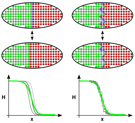
Figure 2: Two different contributions to the intra-embryonic variance in the boundary position. The total variance of the gap gene expression boundary position $x_{\mathrm{t}}$ due to intra-embryonic fluctuations, $\sigma^{2}_{\mathrm{x_{\mathrm{t}},intra}}$, can be decomposed into two contributions: $\sigma^{2}_{\mathrm{\langle x_{\mathrm{t}}\rangle_{\mathrm{\phi}}}}$, the variance in time of the circumferential mean of $x_{\mathrm{t}}$, and $\overline{\sigma^{2}_{\mathrm{x_{\mathrm{t}}}}}$, the time-average of the variance of $x_{\mathrm{t}}$ along the circumference of the embryo. The sketch illustrates two extremal cases: If the boundary is very smooth along the circumference at any moment in time, concerted movements of the boundary will dominate the total variance, i.e. $\sigma^{2}_{\mathrm{x_{\mathrm{t}},intra}}\simeq\sigma^{2}_{\mathrm{\langle x_{\mathrm{t}}\rangle_{\mathrm{\phi}}}}$ (left side). If, in contrast, the boundary is rough but its mean position does not fluctuate much in time, then $\sigma^{2}_{\mathrm{x_{\mathrm{t}},intra}}\simeq\overline{\sigma^{2}_{\mathrm{x_{\mathrm{t}}}}}$ (right side). Naturally, a combination of the two types of fluctuations is possible.

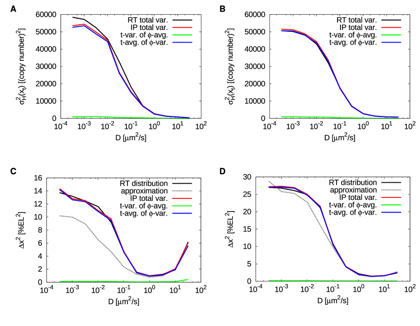
Figure S2: Decomposition of variances at the boundary. (A) Decomposition of the total Hb copy number variance at the average boundary position for the system with mutual repression as a function of the gap protein diffusion constant $D$. Plotted are: $\sigma^{2}_{\mathrm{H}}(x_{\mathrm{t}})$ the total (time- and circumference-) variance measured during runtime (RT, black), the same quantitity determined from a set of 6400 instantaneous profiles (IP, red, 64 AP rows at 100 different time points), $\sigma^{2}_{\mathrm{\langle H\rangle_{\mathrm{\phi}}}}$ the variance in time of the circumference average of $H(x_{\mathrm{t}},\phi)$ (green) and $\overline{\sigma^{2}_{\mathrm{H}}}$ the time average of the variance of $H(x_{\mathrm{t}},\phi)$ over the circumference (blue). (B) The same as (A) for the system without mutual repression. (C) The same variance decomposition as in (A) for the Hb boundary position $x_{\mathrm{t}}$ instead of the copy number. The black line shows the $\Delta x$ values measured as the standard deviation of the boundary position histogram accumulated during runtime (RT), the grey dashed line the corresponding values determined from the approximation $\sigma_{\mathrm{H}}(x_{\mathrm{t}})/|\langle H(x_{\mathrm{t}})\rangle^{\prime}|$. (D) The same as in (C) for the system without mutual repression. In both cases, the main contribution to the total boundary variance $\sigma^{2}_{\mathrm{x_{\mathrm{t}}}}$ comes from $\overline{\sigma^{2}_{\mathrm{x_{\mathrm{t}}}}}$, implying that the blurring of the boundary is rather due to roughness than due to concerted boundary movements.

Intra-embryonic fluctuations. Fig. S2 in Text S1 shows the decomposition of the noise in the Hb copy number $H$ and the threshold position $x_{\mathrm{t}}$ of the Hb boundary, as a function of the diffusion constant. We show the intra-embryonic fluctuations for one given embryo (with the baseline parameter set); how $\Delta x$ (the boundary variance originating from intra-embryonic fluctuations) changes with embryo-to-embryo variations in the morphogen levels is addressed in section “Overlap of morphogen activation domains does not corrupt robustness to intrinsic fluctuations”. Fig. S2 shows that by far the dominant contribution to the intra-embryonic noise in the copy number and threshold position is the time average of the variance in these observables along the circumferential direction; the variance in time of the $\phi$-average of these quantities is indeed very small. The picture that emerges is that the expression boundary is rough, even when the diffusion constant $D$ is large, i.e. $D=1~{}\,\mathrm{\mu m^{2}/s}$. An analysis of the spatial correlation function at midembryo $\overline{\langle{\delta H(0)\delta H(\phi)}\rangle_{\phi}}(x_{\mathrm{t}})$, where $\delta H(\phi)=H(x_{\mathrm{t}},\phi,t)-\overline{\langle{H}\rangle_{\phi}}$, revealed that the correlation length $\xi_{\mathrm{\phi}}$ is on the order of a few nuclei, which corresponds to the diffusion length $\lambda=\sqrt{D/\mu_{\mathrm{eff}}}$ a protein can diffuse with diffusion constant $D$ before it is degraded with a rate $\mu_{\mathrm{eff}}$; the correlation length is thus small compared to the circumference. One possible source of coherent fluctuations in the mean copy number $\langle X\rangle_{\mathrm{\phi}}$ and boundary position $\langle x_{\mathrm{t}}\rangle_{\mathrm{\phi}}$ are temporal variations of the morphogen profiles. However, in our model, these profiles are static—we argued that the morphogen fluctuations are fast on the timescale of gene expression, and are thus effectively integrated out. The small correlation length $\xi_{\mathrm{\phi}}$ then indeed means that the varations in the mean over $\phi$, $\langle\dots\rangle_{\mathrm{\phi}}$, will be small. This leads to an interesting implication for experiments, which we discuss in the Discussion section.

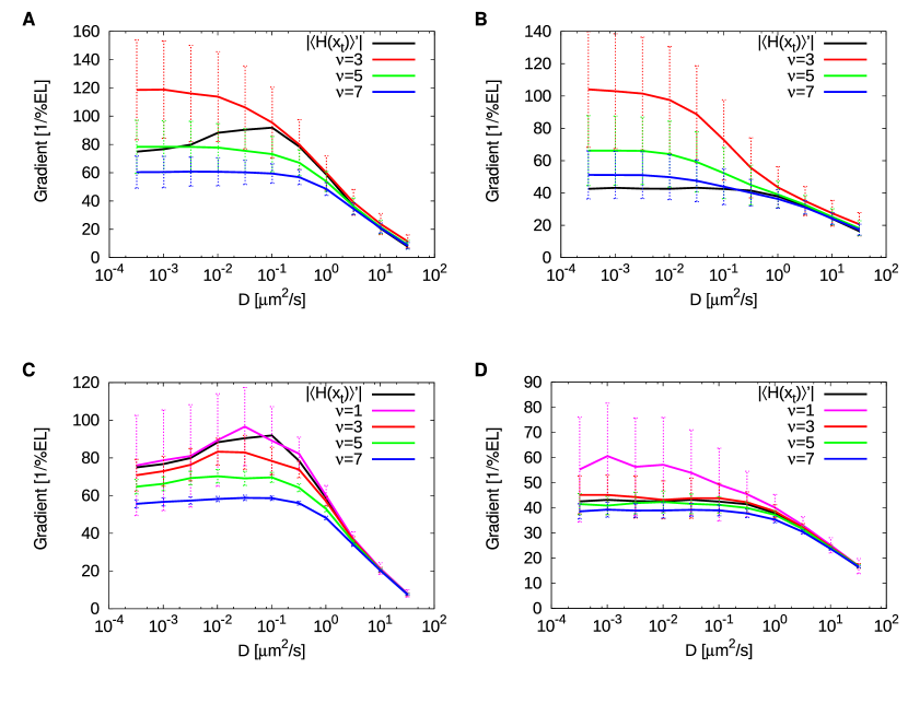
Figure S3: Microscopic properties of the boundary steepness. Panels (A) and (B) compare for different gap protein diffusion constants $D$ the average Hb profile steepness at the boundary measured in a set of 6400 instantaneous profiles (64 AP rows at 100 different time points) to the steepness of the (time- and circumference-) average of the Hb profile ($|\langle H(x_{\mathrm{t}})\rangle^{\prime}|$, black) for different numbers $\nu$ of neighboring data points used in calculating running averages over the instantaneous profiles for the system with (A) and without (B) mutual repression. Although for increasing $\nu$ the instantaneous profiles become less steep as a consequence of the smoothening, the values for $\nu=3$ indicate that the profiles at a given row and time instance are slightly steeper than the average profile. In panels (C) and (D) we show results of the same analysis performed on the 100 circumference-averages of the instantaneous profiles, again for the system with (C) and without (D) mutual repression. Here $\nu=1$ is the data obtained without calculating running averages (magenta). In both systems the steepness of the $\phi$-averaged profiles agrees reasonably well with the steepness of the average profile $|\langle H(x_{\mathrm{t}})\rangle^{\prime}|$.

The boundary steepness. Now that we have characterized the fluctuations in the copy number and the boundary position, the next question is how fluctuations in the copy number affect the steepness of the boundary. In particular, a gene-expression boundary can be shallow either because at each moment in time the interface is shallow, or because at each moment in time the interface is sharp yet the interface fluctuates in time, leading to a smooth profile. The question is thus how much the gradient of the mean concentration profile, $\overline{\langle{G}\rangle_{\phi}}^{\prime}$, and the mean of the gradient, $\overline{\langle{G^{\prime}}\rangle_{\phi}}$, differ (here the prime denotes the spatial derivative). Fig. S3 in Text S1 shows both quantities as a function of the diffusion constant. It is seen that while the average of the gradient is larger than the gradient of the average (as it should), the difference is around a factor of 2. We thus conclude that the steepness of the expression boundary at each moment in time does not differ very much from the steepness of the average concentration profile.

In the rest of the manuscript, we will predominantly focus on the properties of individual embryos, and average quantities are typically averages over time and the circumference. For brevity, therefore, $\langle\dots\rangle=\overline{\langle{\dots}\rangle_{\phi}}$, unless stated otherwise.

Robustness to intra-embryonic fluctuations: Mutual repression allows for steeper profiles without raising the noise level at the boundary

Mutual repression shifts boundaries apart. Fig. 3A shows the average Hb and Kni steady-state profiles along the anterior-posterior (AP) axis as a function of their diffusion constant $D$ for a system with mutual repression. The inset shows the morphogen-activation profiles, which are the spatial profiles of the probability that the hb and kni promoters have 5 copies of their respective morphogens bound. Without mutual repression, thus when Hb and Kni cannot bind to their respective target promoters, these profiles describe the probability that hb and kni are activated by their respective morphogens. Indeed, without mutual repression and without Hb and Kni diffusion, the Hb and Kni concentration profiles would be proportional to their respective morphogen-activation profiles [19], which means that they would precisely intersect at midembryo. In contrast, Fig. 3A shows that the Hb and Kni concentration profiles are shifted apart in the system with mutual repression. There is already a finite separation for $D=0$, which increases further as $D$ is increased.

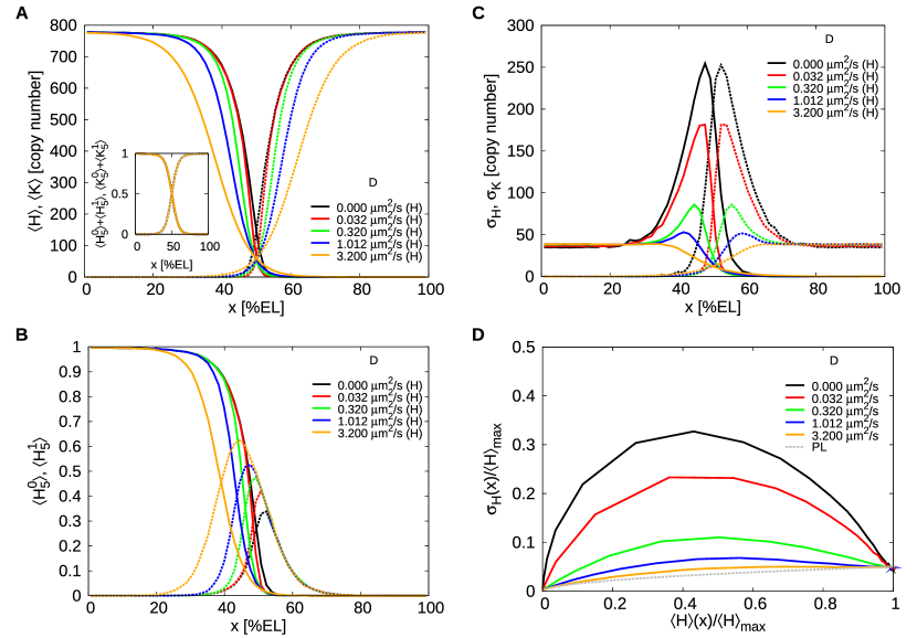
Figure 3: The effect of mutual repression on the average protein concentrations and their standard deviations. (A) Time- and circumference-averaged Hb ($\langle H\rangle$, solid lines) and Kni ($\langle K\rangle$, dashed lines) total protein copy number profiles along the AP axis for various diffusion constants $D$ in a system with mutual repression. The inset shows for both the hb and the kni promoter the probability that the promoter binds 5 morphogen proteins irrespective of whether the antagonistic gap protein is bound to it (meaning that the promoter is activated by the morphogen, even though it may be repressed by the antogonistic gap protein); these “morphogen-activation” profiles are identical for all $D$ values. (B) Profiles of the probability $\langle H^{0}_{\mathrm{5}}\rangle$ that the hb promoter is induced, meaning that it has 5 copies of Bcd bound to it and no Kni dimer (solid lines), and the probability $\langle H^{1}_{\mathrm{5}}\rangle$ that hb is activated by Bcd yet repressed by Kni, in which case hb is indeed not expressed (dashed lines). (C) AP profiles of the time- and circumference-averaged standard deviation of the total gap protein copy number for Hb ($\sigma_{\mathrm{H}}$, solid lines) and Kni ($\sigma_{\mathrm{K}}$, dashed lines). (D) Normalized standard deviation $\sigma_{\mathrm{H}}(x)/\langle H\rangle_{\mathrm{max}}$ versus the normalized mean $\langle H\rangle(x)/\langle H\rangle_{\mathrm{max}}$; $\langle H\rangle(x)$ is the averaged total Hb copy number at $x$ and $\langle H\rangle_{\mathrm{max}}$ is the maximum of this average over all $x$. The grey dashed line represents the Poissonian limit (PL) given by $\sqrt{(1+f_{\mathrm{D}})\langle H\rangle(x)}/\langle H\rangle_{\mathrm{max}}$, where $f_{\mathrm{D}}$ is the fraction of proteins in dimers.

In Fig. 3B we show the profile of the probability $\langle H^{0}_{\mathrm{5}}\rangle$ that the hb promoter is induced, meaning that it has 5 copies of Bcd bound to it and no Kni, and the profile of the likelihood $\langle H^{1}_{\mathrm{5}}\rangle$ that hb is activated by Bcd, yet repressed by Kni, in which case hb is not expressed. It is seen that repression by kni almost fully inhibits hb expression beyond the half-activation point, where hb would be expressed without kni repression (see inset Panel A). Indeed, mutual repression effectively cuts off protein production beyond midembryo. The production probability therefore changes more abruptly along the AP axis, leading to a higher steepness of the protein profiles near midembryo. For $D>0$, repressor influx over the midplane increases, and as a result the regions of expression inhibiton are enlarged and the concentration profiles shift apart further.

Noise reduction via spatial averaging. Fig. 3C shows the standard deviation of the protein copy number along the AP axis for both Hb ($\sigma_{\mathrm{H}}$) and Kni ($\sigma_{\mathrm{K}}$). It is seen that the noise increases close to the half-activation point where promoter-state fluctuations are strongest [46, 47, 48]. This is also observed in Fig. 3D, which shows the normalized standard deviation $\sigma_{\mathrm{H}}/\langle H\rangle_{\mathrm{max}}$ versus the normalized mean $\langle H\rangle/\langle H\rangle_{\mathrm{max}}$ of the average Hb copy number; here, $\langle H\rangle_{\mathrm{max}}$ is the maximum average concentration of Hb. The noise maximum close to mid embryo diminishes with increasing $D$, approaching the Poissonian limit. Note that the Poissonian limit here is given by $\sigma_{\mathrm{P}}=\sqrt{(1+f_{\mathrm{D}})\langle H\rangle}$, where $f_{\mathrm{D}}=2\langle H_{\mathrm{D}}\rangle/\langle H\rangle$ is the fraction of dimerized Hb proteins with respect to the total Hb copy number (see Text S1 for details). Clearly, the spatial averaging mechanism described in [19, 20] reduces the noise also in our system, which differs from those in [19, 20] by the presence of both gap gene monomers and dimers instead of monomers only.

Mutual repression reduces the boundary width by increasing the steepness. Fig. 4 quantifies the impact of spatial averaging and mutual repression on the Hb boundary width $\Delta x$, comparing it to that of the system without mutual repression. To first order, the boundary precision $\Delta x$ is related to the standard deviation in the protein copy number at the boundary, $\sigma_{\mathrm{H}}(x_{\mathrm{t}})$, and the steepness of the boundary, $|\langle H(x_{\mathrm{t}})\rangle^{\prime}|$, via Eq. 1 [35, 6, 19]. The noise $\sigma_{\mathrm{H}}(x_{\mathrm{t}})$ decreases with increasing $D$ due to spatial averaging in an almost identical manner for the systems with and without mutual repression (Fig. 4, top panel); indeed, perhaps surprisingly, mutual repression has little effect on the noise at the boundary. Increasing $D$ also lessens the steepness of the protein profiles, thus reducing the slope $|\langle H(x_{\mathrm{t}})\rangle^{\prime}|$ (Fig. 4, middle panel). While without mutual repression this reduction is monotonic, in the case with mutual repression the steepness first rises because increasing $D$ increases the influx of the antagonistic repressor into the regions where the gap genes are activated by their respective morphogens, which, for low values of $D$, steepens the effective gene-activation profile $\langle H^{1}_{\mathrm{5}}\rangle(x)$ by most strongly reducing gene expression near midembryo; after the steepness has reached its maximum at $D=0.032~{}\,\mathrm{\mu m^{2}/s}$, it drops for higher diffusion constants, because the diffusion of the gap-gene proteins now flattens their concentration profiles. Most importantly, with mutual repression $|\langle H(x_{\mathrm{t}})\rangle^{\prime}|$ reaches significantly higher values for all $D\leq 1.0~{}\,\mathrm{\mu m^{2}/s}$. At $D=0.032~{}\,\mathrm{\mu m^{2}/s}$ the profile is roughly twice as steep as in the case without repression. Interestingly, for $D\lesssim 0.1~{}\,\mathrm{\mu m^{2}/s}$, our simulation results for the steepness of the profiles as normalized by their maximal values agree with those measured experimentally by Surkova et al. in cell cycle 14 [11]: In both simulation and experiment, the concentration drops from 90% to 10% of the maximal values over 5-10% of the embryo length.

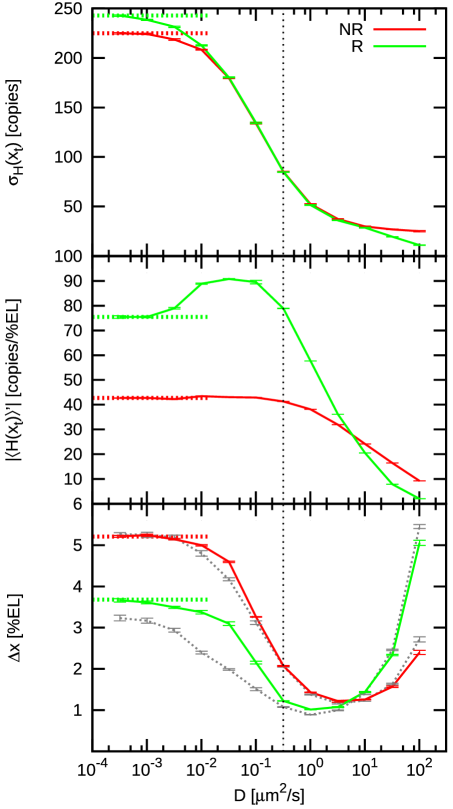
Figure 4: The effect of mutual repression on the precision and steepness of the Hb boundary. The figure shows the time- and circumference-average of the standard deviation of the total Hb copy number at the boundary $\sigma_{\mathrm{H}}(x_{\mathrm{t}})$ (upper panel), the slope of the total Hb copy number profile at the boundary $|\langle H\rangle^{\prime}(x_{\mathrm{t}})|$ (middle panel) and the Hb boundary width $\Delta x$ (lower panel) as a function of the diffusion constant $D$ of the gap proteins. Red solid lines show the case without (NR) and green solid lines the case with mutual repression (R); the red and green dashed lines show the limiting values without diffusion of the gap proteins. The grey dashed lines in the boundary width plot are the values based on the approximation $\Delta x=\sigma_{\mathrm{H}}(x_{\mathrm{t}})/|\langle H(x_{\mathrm{t}})\rangle^{\prime}|$. Note that for $D<3.2~{}\,\mathrm{\mu m^{2}/s}$, mutual repression enhances the steepness of the boundary, which in turn enhances the precision of the boundary. The black dotted line marks the $D$-value where the boundary is both steep and precise due to mutual repression.

Both with and without Hb-Kni mutual repression the trade-off between noise and steepness reduction leads to an optimal diffusion constant $D_{\mathrm{min}}$ that maximizes boundary precision, i.e. minimizes $\Delta x$ (Fig. 4, lower panel). Mutual repression enhances the precision for $D\leq 1.0~{}\,\mathrm{\mu m^{2}/s}$ because in this regime decreasing $D$ increases the steepness markedly while it has only little effect on the noise as compared to the system without mutual repression. Conversely, $\Delta x$ is increased by mutual repression for $D\geq 10~{}\,\mathrm{\mu m^{2}/s}$ because it reduces the steepness. The minimum in the case with repression is marginally lower than that without ($D_{\mathrm{min,R}}/D_{\mathrm{min,NR}}\simeq 0.86$), but located at a lower $D$-value ($1.0~{}\,\mathrm{\mu m^{2}/s}$ vs. $3.2~{}\,\mathrm{\mu m^{2}/s}$). Most importantly, at $D=0.32~{}\,\mathrm{\mu m^{2}/s}$, the system with mutual repression produces a profile that is twice as steep as that of the system without it at $D_{\mathrm{min,NR}}=3.2~{}\,\mathrm{\mu m^{2}/s}$, whereas the precision $\Delta x$ is essentially the same in both cases. Clearly, mutual repression can strongly enhance the steepness of gene-expression boundaries without compromising their precision.

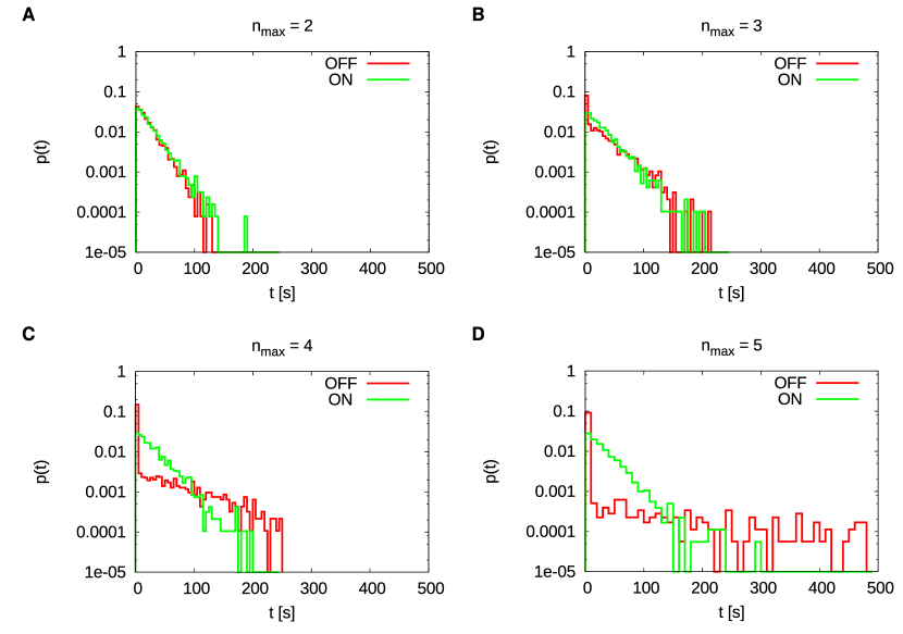
Figure S5: On- and off-times distributions of the hb promoter for different Hill coefficients $n_{max}$ in a nucleus at midembryo. The panels show normalized histograms of the times spent in the producing ($n=n_{max}$) promoter state (“ON”, green) and of the times spent in the non-producing ($n<n_{max}$) states (“OFF”, red) for (A) $n_{max}=2$, (B) $n_{max}=3$, (C) $n_{max}=4$ and (D) $n_{max}=5$ (standard case). It can be seen that with increasing Hill coefficient $n_{max}$ the off-times distribution changes from an exponential to a non-exponential distribution with high weight on very short off-times (implying fast returns to the producing state) and a with a long tail of long off-times. Since the off-rate from the producing state is kept the same for all $n_{max}$ the on-times distributions remain unaltered. The on- and off-times have been determined from long time trajectories ($t_{\mathrm{total}}=10^{5}~{}s$) of the occupancy of the producing state with a sampling resolution of $0.5~{}s$.

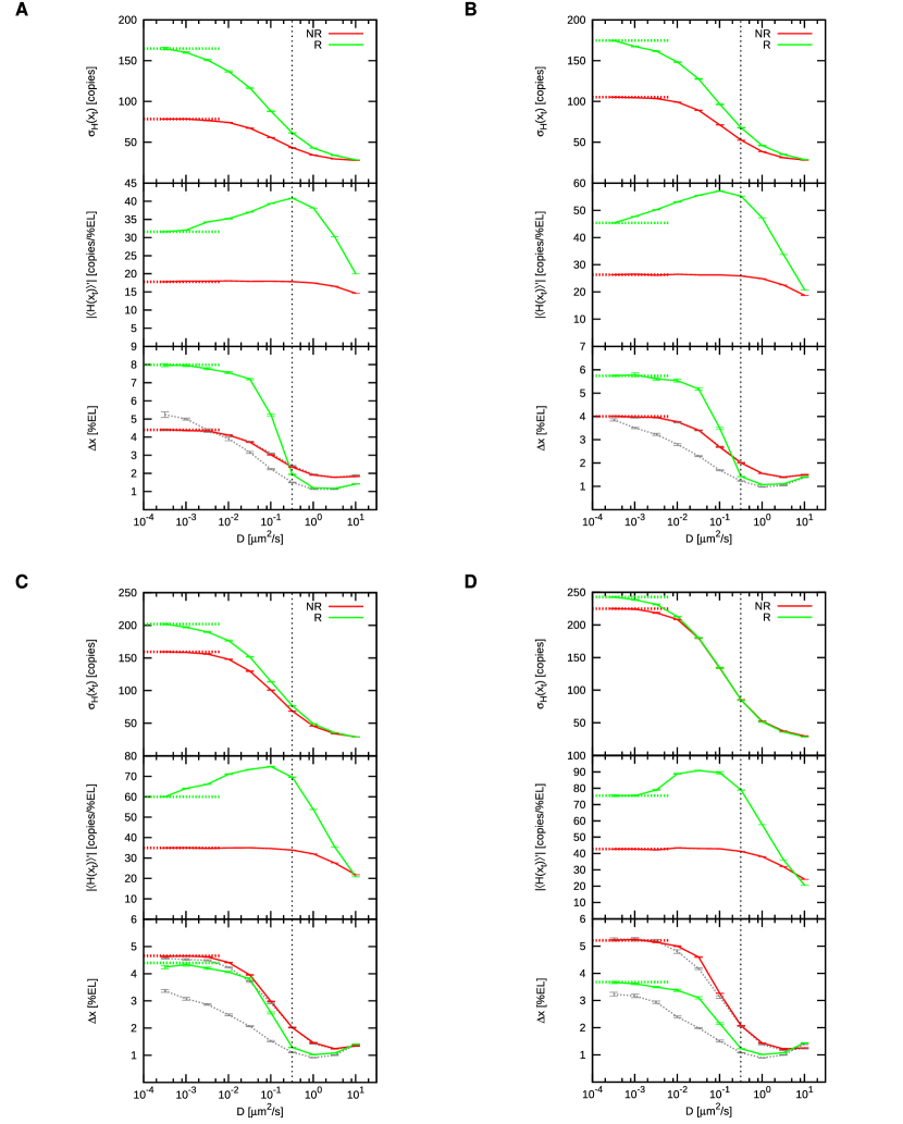
Figure S6: Boundary characteristics for reduced Hill coefficients $n_{max}$. See following page for description.

Influence of Hill coefficient. A key parameter controlling the precision of the gap-gene expression boundaries, is the degree of cooperativity by which the gap genes are activated by their respective morphogens—this determines the profile steepness of the average gap-gene promoter activity. To investigate this, we have lowered the effective Hill coefficient from its baseline value of 5 by reducing the number $n_{\mathrm{\rm max}}$ of morphogen molecules that are required to bind the promoter to activate gene expression. To isolate the effect of varying the mean gene-activation profiles $\langle H_{\mathrm{n_{\mathrm{\rm max}}}}^{0}\rangle(x)$ and $\langle K_{\mathrm{n_{\mathrm{\rm max}}}}^{0}\rangle(x)$, we varied, upon varying $n_{\mathrm{\rm max}}$, the association and dissociation rates such that 1) the average gene activation probabilities near midembryo, $\langle H_{\mathrm{n_{\mathrm{\rm max}}}}^{0}\rangle(L/2)$ and $\langle K_{\mathrm{n_{\mathrm{\rm max}}}}^{0}\rangle(L/2)$, are unchanged and 2) the waiting-time distribution for the gene on-to-off transition is unchanged (since the average activation probability is fixed, the mean off-to-on rate is also unchanged, although the waiting-time distribution is not; see also Fig. S5 in Text S1). We observe that mutual repression markedly enhances the steepness of the gap-gene expression boundaries, also with a lower Hill coefficient for gene activation (Fig. S6 in Text S1). However, lowering the Hill coefficient reduces the steepness of the gene-activation profiles, causing the two antagonistic gene-activation profiles to overlap more. As a result, in each of the two gap-gene expression domains, more of the antagonist is present, which tends to increase the noise in gene expression by occassionally shutting off gene production. This, as explained in more detail later, is particularly detrimental when the diffusion constant is low. Indeed, when the effective Hill coefficient of gene activation is 3 or lower, mutual repression increases $\Delta x$ when the diffusion constant is low, i.e. below approximately $0.1~{}\,\mathrm{\mu m^{2}/s}$. Nonetheless, the minimal $\Delta x$ is still lower with mutual repression, and, consequently, also with a lower Hill coefficient for gene activation, mutual repression can enhance both the steepness and the precision of gene-expression boundaries.

Influence of the repression strength. As a standard we assume very tight binding of the Hb and Kni dimers, “the repressors”, to their respective promoters. To test how this assumption affects our results we performed simulations in which we systematically varied the repressor-promoter dissociation rate $k^{\rm R}_{\mathrm{off}}$ in the range $[5.27\cdot 10^{-4}\,\mathrm{/s},5.27\cdot 10^{2}\,\mathrm{/s}]$, keeping the diffusion constant at $D=1.0~{}\,\mathrm{\mu m^{2}/s}$ (the value that minimizes the boundary width at $k^{\rm R}_{\mathrm{off}}=5.27\cdot 10^{-3}\,\mathrm{/s}$) and all other parameters the same as before. Fig. 5 shows the noise, steepness and boundary precision as a function of the repressor-promoter dissociation rate. For high dissociation rates, these quantities equal those in the system without mutual repression (dashed lines). Yet, as the dissociation rate is decreased, the steepness rises markedly at $k^{\rm R}_{\mathrm{off}}=1/{\rm s}$. In contrast, the noise $\sigma_{\mathrm{H}}(x_{\mathrm{t}})$ first decreases with decreasing $k^{\rm R}_{\mathrm{off}}$, passing through a minimum at $k^{\rm R}_{\mathrm{off}}=0.1/{\rm s}$ before rising to a level that is higher than that in a system without mutual repression. This minimum arises because on the one hand increasing the affinity of the repressor (the antagonist) makes the operator-state fluctuations of the activator (the morphogen) less important—increasing repressor binding drives the concentration profiles of Hb and Kni away from midembryo, where the promoter-state fluctuations of the activators are strongest; on the other hand, when the repressor binds too strongly, then slow repressor unbinding leads to long-lived promoter states where gene expression is shut off, increasing noise in gene expression; this phenomenon is similar to what has been observed in Refs. [47] and [49], where slower binding of the gene regulatory proteins to the promoter increases noise in gene expression and decreases the stability of a toggle switch, respectively. The interplay between the noise and the steepness yields a marked reduction of the boundary width $\Delta x$; indeed, even in the limit of very tight repressor binding, mutual repression significantly enhances the precision of the boundary.

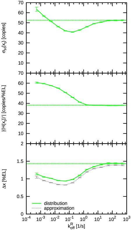
Figure 5: The effect of varying repression strength on the precision and steepness of the Hb boundary. Shown are the time- and circumference average of the standard deviation of the total Hb copy number at the boundary $\sigma_{\mathrm{H}}(x_{\mathrm{t}})$ (upper panel), the steepness of the boundary $|\langle H\rangle^{\prime}(x_{\mathrm{t}})|$ (middle panel) and the Hb boundary width $\Delta x$ (lower panel) as a function of $k_{\mathrm{\rm off}}^{\rm R}$, the promoter-dissociation rate of Hb and Kni. The solid green line are values obtained from the boundary position distribution, the dashed grey line the ones calculated from the approximation $\Delta x=\sigma_{\mathrm{H}}(x_{\mathrm{t}})/|\langle H(x_{\mathrm{t}})\rangle^{\prime}|$. Straight dashed lines mark the limits for the case without mutual repression ($k_{\mathrm{on}}^{\rm R}=k_{\mathrm{off}}^{\rm R}=0$).

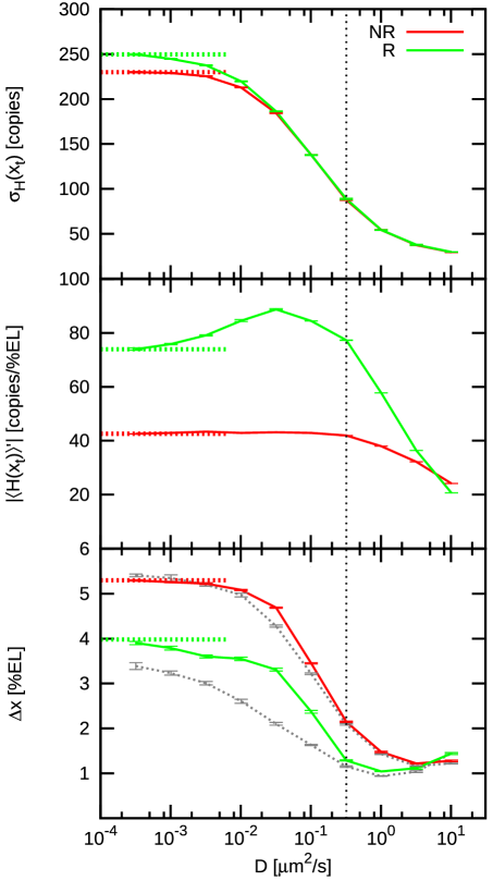
Figure S8: The effect of bursty gap protein production on the Hb boundary precision. The plot shows $\sigma_{\mathrm{H}}(x_{\mathrm{t}})$ the standard deviation of the total Hb copy number at the boundary, the steepness $|\langle H(x_{\mathrm{t}})\rangle^{\prime}|$ of the average total Hb copy number profile at the boundary and the boundary width $\Delta x$ with (green) and without (red) mutual repression as a function of the gap protein diffusion constant $D$ for a system in which the gap proteins are produced in bursts of 10 at a time with decreased production rate $\beta=\beta_{\mathrm{0}}/10$. The grey dashed lines are the values obtained from the approximation $\Delta x=\sigma_{\mathrm{H}}(x_{\mathrm{t}})/|\langle H(x_{\mathrm{t}})\rangle^{\prime}|$. Thick dashed lines are values for $D=0$. Error bars were obtained from block averages over 10 independent samples. The black dotted line marks the $D$-value where the boundary is both steep and precise due to mutual repression.

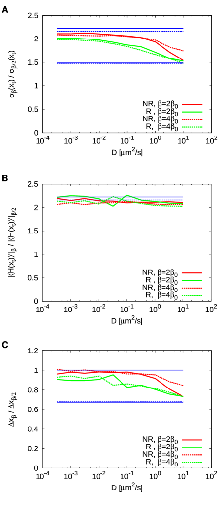
Figure S9: The effect of increased copy number on the Hb boundary precision. See following page for description.

Influence of expression level. Since the precise gap protein expression level is not known, we also varied the maximal protein copy number $N$ by varying the maximal expression rate $\beta$ (see Text S1). Fig. S9 in Text S1 shows the output noise and slope at the boundary position, and the boundary precision $\Delta x$, as a function of the diffusion constant for three different expression levels. It is seen that for low diffusion constant, the precision is independent of $N$, while for higher diffusion constant it scales roughly with $1/\sqrt{N}$. This can be understood by noting that the steepness of the gene-expression boundary scales to a good approximation with $N$ independently of $D$, while the noise $\sigma$ scales with $N$ when the diffusion constant is small, but with $\sqrt{N}$ when the diffusion constant is large (see also Eq. 1). The scaling of the noise with $N$ is due to the fact that for low $D$ the noise in the copy number is dominated by the noise coming from the promoter-state fluctuations, which scales linearly with $N$, while for high $D$, diffusion washes out the expression bursts resulting from the promoter-state flucutations, leaving only the noise coming from the Poissonian fluctuations arising from transcription and translation, which scales with the square root of $N$ [19]. In Text S1 we also study the importance of bursts arising in the transcription-translation step (see Fig. S8 in Text S1); however, we find that for a typical burst size, these bursts do not dramatically affect boundary precision.

Robustness to inter-embryonic variations: Mutual repression can buffer against correlated morphogen level variations

Although the Bcd copy number at midembryo has been determined experimentally [6], the measured value is not necessarily the half-activation threshold of hb. Indeed, in vivo the Hb profile is shaped by other forces, like mutual repression. In the kni-kr double mutant, the Hb boundary at midembryo shifts posteriorly [13]. Moreover, gap gene domain formation has been observed at strongly reduced Bcd levels, suggesting that Bcd might be present in excess [50]. Also from a theoretical point of view it is not obvious that a precisely centered morphogen-activation threshold is optimal, in terms of robustness against both intra-embryonic fluctuations and inter-embryonic variations. Here, we study the effect of changing the threshold position where hb and kni are half-maximally activated by their respective morphogens, Bcd and Cad. While the threshold positions could be varied by changing the threshold morphogen concentrations for half-maximal gap-gene activation (for example by changing the morphogen-promoter dissociation rates), we will vary these positions by changing the amplitude of the morphogen profiles by a factor $A$. This procedure not only preserves the promoter-activation dynamics at the boundaries—a key determinant for the noise at the boundaries—but also allows us to study the importance of mutual repression in ensuring robustness against embryo-to-embryo variations. Indeed, we will examine not only how changing the threshold position affects the precision of the gap-gene expression boundaries, $\Delta x(A)$, but also how the average boundary positions vary with morphogen dosage, $x_{\mathrm{t}}(A)$, and how the latter gives rise to embryo-to-embryo variations in the boundary position $\Delta x_{\mathrm{t}}(\Delta A)$ due to embryo-to-embryo variations in the morphogen dosage $\Delta A$.

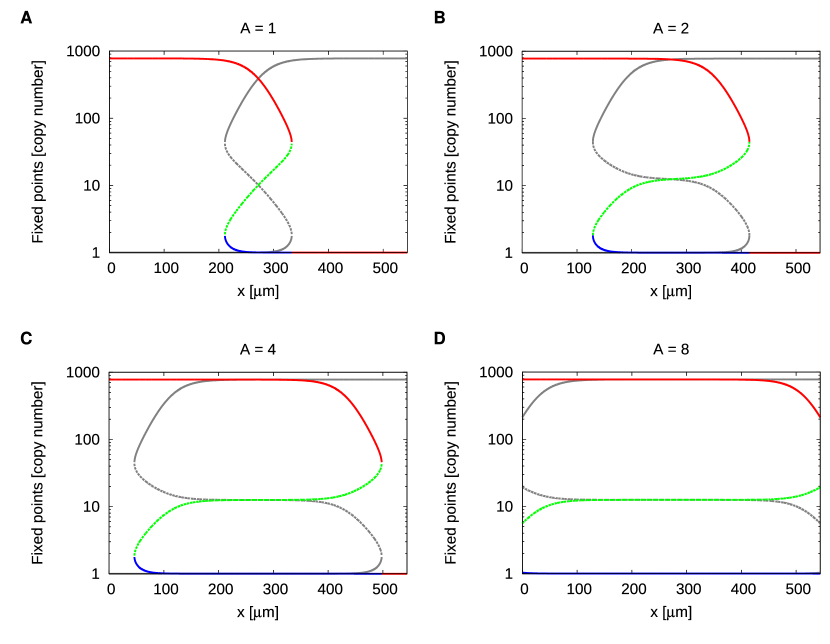
Figure S1: Bifurcation analysis of a one dimensional mean-field model of mutually repressing gap genes activated by morphogen gradients. Plotted are the stable (solid lines) and unstable (dashed lines) fixed points of the copy number of Hb (colored lines) and Kni (grey lines) as a function of the AP position $x$ as predicted by a bifurcation analysis performed on a 1D mean-field model in which hb and kni are activated cooperatively by their respective morphogens and mutually repressing each other. Different colors correspond to different fixed points. The different panels show the solutions for activator amplitudes (A) A=1, (B) A=2, (C) A=4 and (D) A=8. All other parameters values are the standard values from Table S2. Activator concentrations at position $x$ used in the mean-field analysis correspond to the ones in the 2D stochastic simulations. Away from midembryo each gap protein level has only one stable fixed point and one of the two levels is always zero. For all $A$ there is a region around midembryo in which the protein levels have two stable and one unstable fixed point, implying bistability. In this region the analysis predicts bistable switching between the high-Hb–low-Kni and the low-Hb–high-Kni state. For clarity we color-code the Hb fixed points only. The Kni solutions are identical to the Hb solutions mirrored with respect to midembryo.

Double-activation induces bistability. We first consider the scenario in which the amplitudes of both morphogens are scaled by the same factor $A$. When $A=1$, the position at which hb and kni are half-maximally activated by their respective morphogens coincide at midembryo, meaning that the domains in which hb and kni are activated beyond half-maximum are adjoining, but do not overlap—this is the scenario discussed in the previous sections. When $A>1$, the position at which hb is half-maximally activated by its morphogen is shifted posteriorly, while that of kni is shifted anteriorly, creating an overlap between the two regions where hb and kni are activated. In this “double-activated region” both hb and kni are activated by their respective morphogens, yet they also mutually repress each other. This may lead to bistability. To probe whether this is the case, we performed a bifurcation analysis of the mean-field chemical-rate equations of isolated nuclei, implying that $D=0$ (see Fig. S1 in Text S1). In addition, we performed stochastic simulations of isolated nuclei with different morphogen levels corresponding to different positions along the AP axis. All other parameter values were the same as in the full-scale simulation. We recorded long trajectories of the order parameter $\Delta N\equiv H-K$, the difference between the total Hb and total Kni copy numbers, in the stationary state. From each trajectory we computed the distribution $P(\Delta N)$ of the probability that the system is in a state with copy number difference $\Delta N$. This defines a “free energy” $G(\Delta N)\equiv-\ln P(\Delta N)$, with minima of $G(\Delta N)$ corresponding to maximally probable values of $\Delta N$ [26, 27]. For a bistable system, $G(\Delta N)$ resembles a double-well potential with minima located at a positive value of $\Delta N=\Delta N_{\mathrm{\rm H}}$ and a negative value of $\Delta N=\Delta N_{\mathrm{\rm K}}$, respectively. At midembryo the morphogen levels of Bcd and Cad are the same and hence the biochemical network in the nuclei in the midplane is symmetric, which means that, if this network is bistable, $G(\Delta N)$ resembles a symmetric double-well potential with $\Delta N_{\mathrm{H}}=-\Delta N_{\mathrm{K}}$ and $\Delta G\equiv G(\Delta N_{\mathrm{H}})-G(\Delta N_{\mathrm{K}})=0$. Away from the middle, the morphogen levels differ, and one state will become more stable than the other; if the other state is, however, still metastable, then $G(\Delta N)$ will resemble an asymmetric double-well potential, with $\Delta G$ being negative if the hb-dominant state is more stable than the kni-dominant state, and vice versa. The emergence of such a “spatial switch” along the AP axis is also captured by our mean-field, bifurcation analysis (see Text S1) and was recently also shown in the mean-field analysis of Papatsenko and Levine for the same pair of mutually repressing genes[28].

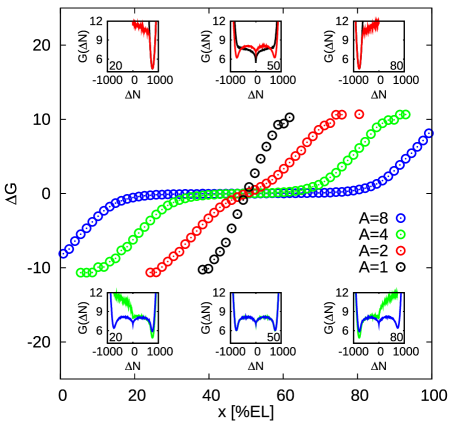
Figure 6: Emergence of bistability in double-activated regions. The “free energy” difference $\Delta G\equiv G(\Delta N_{\mathrm{H}})-G(\Delta N_{\mathrm{K}})$ as a function of $x$, the distance of the nucleus from the anterior pole, for different amplitudes of the morphogen gradients $A$; here, $G(\Delta N)\equiv-\ln(P(\Delta N))$, where $P(\Delta N)$ is the stationary distribution of the order parameter $\Delta N=H-K$; $\Delta N_{\mathrm{H}}\simeq-\Delta N_{\mathrm{K}}\approx 800$ correspond to the minima of $G(\Delta N)$. Negative values of $\Delta G$ represent a strong bias towards the high-Hb state, while positive values correspond to high-Kni states. The insets shows $G(\Delta N)$ as a function of $\Delta N$ at the positions indicated by the numbers in their corners (values in [$\,\mathrm{\%EL}$]; colors correspond to main plot). The data is obtained from simulations of single nuclei with morphogen levels corresponding to the ones at position $x$ in the full system; this is equivalent to the full system without diffusion between neighboring nuclei. Note the bistable behavior in a wide region of the embryo for higher $A$ values.

Fig. 6 shows $\Delta G$ as a function of the position along the AP axis, for different amplitudes $A$ of the morphogen gradients. The inset shows the energy profiles $G(\Delta N)$ for different positions along the AP axis. For $A=1$, $G(\Delta N)$ always exhibits one minimum only, irrespective of the position along the AP axis; at midembryo, this minimum is located at $\Delta N=0$, while moving towards the anterior (posterior) the energy minimum rapidly shifts to $\Delta N\approx+800(-800)$, reflecting that in the anterior (posterior) half of the embryo hb (kni) is essentially fully expressed. For $A=2$, $G(\Delta N)$ develops into a double-well potential at midembryo, with two pronounced minima at $\Delta N\approx 800$ and $\Delta N\approx-800$, respectively. These two minima correspond to a state in which hb is highly expressed ($\langle H\rangle\approx 800$) and kni is strongly repressed ($\langle K\rangle\approx 0$) and another state in which kni is highly expressed and hb strongly repressed, respectively. The fact that the two energy mimima are equal indicates that both of these states are equally likely. Moving away from midembryo, however, one gap-gene expression state rapidly becomes more stable than the other, and bistability is lost, yielding a potential with one minimum located at $\Delta N\approx 800$ in the anterior half and a potential with one minimum located at $\Delta N\approx-800$ in the posterior half of the embryo. Interestingly, for $A=4$ and $A=8$ a wide region of bistability develops around midembryo. In this region, $\Delta G\approx 0$, meaning that the high-hb—low-kni state and the low-hb—high-kni state are equally stable. These two states are equally likely because in this region both the hb and kni promoters are fully activated by their respective morphogens. It can also be seen that the width of this bistable region increases with the amplitude of the morphogen gradients, as expected.

Slow switching ensures a low noise level while diffusion avoids error locking. The bistability observed for $A>1$ and $D=0$ raises an important question, namely whether the nuclei can switch between the two gap-gene expression states on the time scale of embryonic development. This question is particularly pertinent for the higher morphogen amplitudes, where these two states are equally likely ($\Delta G\approx 0$) over a wide region of the embryo (Fig. 6): random switching between the two distinct gap-gene expression states in this wide region would then lead to dramatic fluctuations in the positions of the hb and kni expression boundaries, which clearly would be detrimental for development. We therefore computed [27] from the recorded switching trajectories the average waiting time for switching, $\tau_{\mathrm{s}}$, at midembryo ($\Delta G\simeq 0$) for different values of $A$; for $A\geq 2$, we find $\tau_{\mathrm{s}}\simeq 6~{}\,\mathrm{h}$ (see Table S1 in Text S1). During cell cycle 14, approximately 2-3 hours after fertilization, the Bcd gradient disappears [51], suggesting that the spontaneous switching rate is indeed low on the relevant time scale of development.

With diffusion of Hb and Kni between neighboring nuclei ($D>0$), the time scale for switching will be even longer. Diffusion couples neighboring nuclei, creating larger spatial domains with the same gap-gene expression state. This reduces the probability that a nucleus in the overlap region flips to the other gap-gene expression state. The latter can be understood from the extensive studies on the switching behavior of the “general toggle switch” [26, 27, 52, 53, 54, 49], which is highly similar to the system studied here—indeed, the toggle switch consists of two genes that mutually repress each other. These studies have revealed that the ensemble of transition states, which separate the two stable states, is dominated by configurations where both antagonistic proteins are present in low copy numbers. Clearly, the probability that in a given nucleus not only the minority gap protein, but also the majority gap protein reaches a low copy number, is reduced by the diffusive influx of that majority species from the neighboring nuclei, which are in the same gap-gene expression state. In essence, diffusion increases the effective system size, with its spatial dimension given by $\lambda=\sqrt{D/\mu_{\mathrm{\rm eff}}}$; in fact, since the stability of the toggle switch depends exponentially on the system size [26, 27], we expect the stability $\tau_{\mathrm{s}}$ to scale with the diffusion constant as $\tau_{\mathrm{s}}\sim e^{D}$. We thus conclude that random switching between the two gap-gene expression states, the high-hb—low-kni and low-hb—high-kni states, is not likely to occur on the time scale of early development.

The observation that the switching rate is low raises another important question: if errors are formed during development, can they be corrected? We observe in the simulations with $D=0$ that when we allow the gap-gene expression patterns to develop starting from initial conditions in which the Hb and Kni copy numbers are both zero, in the overlap (bistable) region a spotty gap-gene expression pattern emerges, consisting of nuclei that are either in the high-hb—low-kni state or in the low-hb—high-kni state. When the diffusion constant of Hb and Kni is zero, then these defects are essentially frozen in, precisely because of the low switching rate. Interestingly, however, we find in the simulations that a finite diffusion constant can anneal these defects. This may seem to contradict the statement made above that diffusion lowers the switching rate. The resolution of this paradox is that while diffusion lowers the switching rate for nuclei that are surrounded by nuclei that are in the same gap-gene expression state, it enhances the switching rate for nuclei that are surrounded by nuclei with a different gap-gene expression state; this is indeed akin to spins in an Ising system below the critical point. The mechanism for the formation of the gap-gene expression patterns, then, depends on the diffusion constant. When $D$ is small yet finite, $0<D<0.1\,\mathrm{\mu m^{2}/s}$, in the overlap region first small domains are formed consisting of nuclei that are in the same gap-gene expression state; these domains then coarsen analogously to Ostwald ripening of small crystallites in a liquid below the freezing temperature; ultimately, they combine with the hb or kni expression domains that have formed in the meantime outside the overlap region, where hb and kni are activated by their respective morphogens yet do not repress each other (see Videos S1 and S2). For $D\gtrsim 0.1\,\mathrm{\mu m^{2}/s}$, no “crystallites” are formed in the overlap region (both the Hb and Kni copy numbers are low yet finite and hb and kni simultatenously repress each other); instead, the hb and kni domains formed near the poles slowly invade the overlap region (see Videos S3 and S4). Interestingly, even while in the absence of Hb and Kni diffusion $\Delta G\approx 0$ in the overlap region, the interface between the hb and kni expression domains does slowly diffuse towards midembryo when $D>0$ and $A\leq 4$, due to the diffusive influx of Hb and Kni from the regions outside the overlap region. When $A=8$, the hb and kni expression boundaries are not pinned to the middle of the embryo, and their positions exhibit slow and large fluctuations, presumably because the energetic driving force is small, and the diffusive influx of Hb and Kni from the regions near the poles is negligible. We will investigate this effect in more detail in a forthcoming publication.

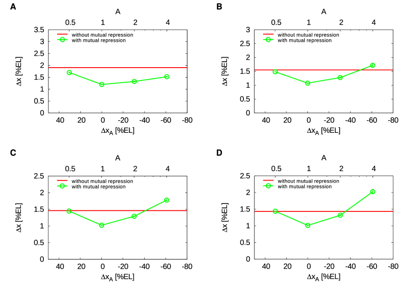
Figure S7: The effect of changing the activator amplitude $A$ on the boundary precision for reduced Hill coefficients $n_{max}$. Shown are the the boundary width $\Delta x$ with (green) and without (red) mutual repression as a function of $\Delta x_{\mathrm{A}}$, the separation between the Hb and Kni boundaries expected in the system without mutual repression, and the corresponding activator amplitude $A$ for Hill coefficients (A) $n_{max}=2$, (B) $n_{max}=3$, (C) $n_{max}=4$ and (D) $n_{max}=5$ (standard case). In all cases $D=1.0~{}\,\mathrm{\mu m^{2}/s}$.

Mutual repression inhibits boundary shifts. Fig. 7A shows the average gap-gene expression profiles for $A\in\{1,2,4\}$ and $D=1.0~{}\,\mathrm{\mu m^{2}/s}$, which minimizes the boundary width $\Delta x$ when $A=1$ (see Fig. 4). While the morphogen-activation thresholds shift beyond midembryo as $A$ is increased beyond unity, leading to an overlap of the domains where the gap genes are activated by their respective morphogens (see inset), the gap-gene expression boundaries overlap only marginally. This is quantified in panel B, which shows the Hb boundary position $x_{\mathrm{t}}$ as a function of $A$ and as a function of $\Delta x_{\mathrm{A}}\equiv x_{\mathrm{A,Kni}}-x_{\mathrm{A,Hb}}$, which is defined as the separation between the positions $x_{\mathrm{A,Kni}}$ and $x_{\mathrm{A,Hb}}$ where Kni and Hb are half-maximally activated by their respective morphogens; for $A=1$, with adjoining morphogen activation regions, $\Delta x_{\mathrm{A}}=0$ and for $A>1$, with overlapping activation regions, $\Delta x_{\mathrm{A}}$ is negative. Without mutual repression (red data), the Hb boundary position $x_{\mathrm{t}}$ tracks the shift of the hb activation threshold, as expected. In contrast, with mutual repression (green data) the boundary does not move beyond the position for $A=1$ as $A$ is increased. The same robustness was also observed for other values of the Hill coefficient of gap-gene activation (see Fig. S7 in Text S1).

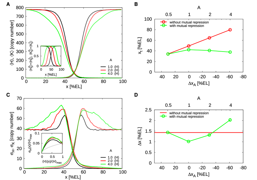
Figure 7: Mutual repression buffers against correlated variations in the activator levels. (A) Time- and circumference-averaged Hb ($\langle H\rangle$, solid lines) and Kni ($\langle K\rangle$, dashed lines) total copy-number profiles along the AP axis for various morphogen dosage factors $A$. Inset: the corresponding average occupancy of the promoter states with five bound morphogen molecules as a function of $x$. (B) The average Hb boundary position $x_{\mathrm{t}}$ as a function of $\Delta x_{\mathrm{A}}$, the distance between the Hb and Kni boundaries without mutual repression, for the system with mutual repression (green,) and without it (red); $\Delta x_{\mathrm{A}}$ is varied by changing the morphogen dosage factor $A$. Note that mutual repression makes the gap-gene expression boundaries essentially insensitive to correlated changes in morphogen levels when $A>1$. (C) AP profiles of the average standard deviation of the total Hb ($\sigma_{\mathrm{H}}$, solid lines) and Kni ($\sigma_{\mathrm{K}}$, dashed lines) copy numbers. Inset: $\sigma_{\mathrm{H}}(x)/\langle H\rangle_{\mathrm{max}}$ as a function of $\langle H\rangle(x)/\langle H\rangle_{\mathrm{max}}$, where $\langle H\rangle(x)$ is the average Hb copy number at $x$ and $\langle H\rangle_{\mathrm{max}}$ its maximum over $x$. The grey dashed line represents the Poissonian limit.(D) The Hb boundary width $\Delta x$ as a function of $\Delta x_{\mathrm{A}}$ with (green) and without (red) mutual repression. For $A=4$, it was impossible to obtain a reliable error bar on $\Delta x$, because of the weak pinning force on the hb and kni expression boundaries.

Mutual repression enhances robustness to embryo-to-embryo variations. The fact that mutual repression can pin expression boundaries, dramatically enhances the robustness against embryo-to-embryo variations in the morphogen levels. We did not sample inter-embryo variations in $A$ explicitly, but made an estimate using $\Delta x_{\mathrm{t}}=(dx_{\mathrm{t}}/dA)\Delta A$, where $dx_{\mathrm{t}}/dA$ was taken from Fig. 7B. A correlated symmetric variation $\delta_{\mathrm{A}}\equiv\Delta A/A=0.1$ of both morphogen levels then would lead to $\Delta x_{\mathrm{t}}(\delta_{\mathrm{A}})\simeq 0.82~{}\,\mathrm{\%EL}$ at $A=1$ and $\Delta x_{\mathrm{t}}(\delta_{\mathrm{A}})\simeq 0.25~{}\,\mathrm{\%EL}$ at $A=2$. Without mutual repression $\Delta x_{\mathrm{t,NR}}(\delta_{\mathrm{A}})\simeq 2.2~{}\,\mathrm{\%EL}$. This analysis thus suggests that mutual repression reduces boundary variations due to fluctuations in the morphogen levels by almost a factor of 10 if the half-activation threshold is slightly posterior to midembryo (e.g. $A=2$). If, on average, $A=1$, then mutual repression still reduces $\Delta x_{\mathrm{t}}$ by inhibiting posterior shifts in those embryos in which $A>1$. These results are consistent with those of [36, 14].

Overlap of morphogen activation domains does not corrupt robustness to intrinsic fluctuations. While mutual repression proves beneficial in buffering against embryo-to-embryo variations in morphogen levels, the question arises whether overlapping morphogen-activation domains does not impair robustness to intrinsic fluctuations arising from noisy gene expression and diffusion of gap gene proteins. We found that this depends on the Hill coefficient of gap-gene activation, which depends on the number $n_{\mathrm{\rm max}}$ of morphogen binding sites on the promoter. Fig. 7C shows, for $n_{\mathrm{\rm max}}=5$, that even though mutual repression increases the noise in gap-gene expression away from the boundaries, it has little effect on the noise at the boundaries when $A\leq 2$. For $A>2$, the noise does increase significantly; in fact, it was impossible to obtain reliable error bars, because of the weak pinning force of the hb-kni interface. Moreover, overlapping morphogen activation domains decrease the steepness of the expression boundaries (panel A), and this increases the boundary width $\Delta x$ (panel D). Indeed, when $n_{\mathrm{\rm max}}=5$, mutual repression can enhance the precision of gene-expression boundaries, but only if the activation domains are adjoining ($A=1$), or have a marginal overlap ($1<A<2$). For lower values of $n_{\mathrm{\rm max}}$, however, this enhancement of precision extends over a much broader range of $A$ values; in fact, when $n_{\mathrm{\rm max}}<3$, mutual repression enhances precision even up to $A=4$ (see Fig. S7 in Text S1).

Boundaries shift upon uncorrelated variations in morphogen levels, yet intrinsic noise remains unaltered

Since correlated upregulation of both morphogen levels is a special case, we also studied the effect of uncorrelated activator scaling. To this end, only the Bcd level was multiplied by a global factor $A\in\{0.5,1,2,3,4\}$, while other parameters were left unchanged. Again we investigated the Hb boundary position $x_{\mathrm{t}}$, its variance $\Delta x_{\mathrm{t}}(\Delta A)$ due to extrinsic (embryo-to-embryo) variations in $A$ and the variance due to intrinsic (intra-embryo) fluctuations $\Delta x(A)$. Results for $D=1.0\,\mathrm{\mu m^{2}/s}$ are summarized in Fig. 8.

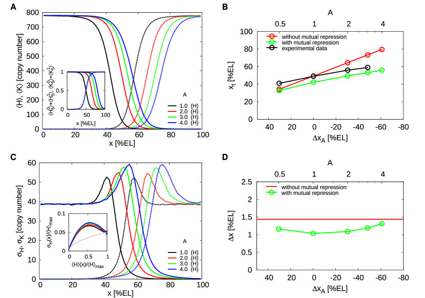
Figure 8: Robustness of the gap-gene expression boundaries to variations in the bcd gene dosage. (A) Time- and circumference-averaged Hb ($\langle H\rangle$, solid lines) and Kni ($\langle K\rangle$, dashed lines) total copy-nymber profiles along the AP axis for various bcd gene dosage factors $A_{\mathrm{Bcd}}=A\in\{0.5,1,2,3,4\}$ and $D=1.0~{}\,\mathrm{\mu m^{2}/s}$. Inset: the average occupancy of the promoter states with five bound morphogen molecules as a function of $x$. (B) Comparison of the boundary position $x_{\mathrm{t}}$ as a function of $A$ for $D=1.0~{}\,\mathrm{\mu m^{2}/s}$ to values measured by Houchmanzadeh et al. [5] (black line). The red line shows the simulation results for the system without mutual repression. Note the good agreement between the experimental data and the simulation data of the system with mutual repression. (C) Profiles of the average standard deviation of the total Hb ($\sigma_{\mathrm{H}}$, solid lines) and Kni ($\sigma_{\mathrm{K}}$, dashed lines) copy number. Inset: $\sigma_{\mathrm{H}}(x)/\langle H\rangle_{\mathrm{max}}$ as a function of $\langle H\rangle(x)/\langle H\rangle_{\mathrm{max}}$. The grey dashed line represents the Poissonian limit. (D) The Hb boundary width $\Delta x$ as a function of $A$ and $\Delta x_{\mathrm{A}}$, the separation between the Hb and Kni boundaries in a system without mutual repression, for the system with (green) and without (red) mutual repression. $\Delta x_{\mathrm{A}}$ is varied by multiplying the Bcd level by $A_{\mathrm{Bcd}}$.

The Hb boundary shifts less with mutual repression. Fig. 8A shows that the hb expression boundary shifts posteriorly with increasing $A$, in contrast to the case of correlated activator scaling. The Kni profile retracts in concert with the advance of the Hb domain. In Fig. 8B we compare the Hb boundary $x_{\mathrm{t}}(A)$ to the data of Houchmandzadeh et al. [5], assuming a 100% efficiency of the additional bcd gene copies. It is seen that the agreement between simulation and experiment is very good: while $x_{\mathrm{t}}(A)$ of the simulations has a marginal offset as compared to the experimental data, the slope of $x_{\mathrm{t}}(A)$ is essentially the same. Moreover, the slope is much lower than that obtained without mutual repression, showing that mutual repression can indeed buffer against uncorrelated variations in morphogen levels. These results parallel those of [36].

Robustness to inter-embryo fluctuations. To estimate the boundary variance due to inter-embryo variations in morphogen levels, we fitted a generic logarithmic function $x_{\mathrm{t,fit}}(A):=a\log(A)+b$ to the simulation data, giving $a\lesssim 15~{}\,\mathrm{\%EL}$ for all values of $D$ studied. Hence $\Delta x_{\mathrm{t}}(\Delta A)\lesssim 15~{}\,\mathrm{\%EL}~{}\Delta A/A$. A $10\%$ variability in $A$ around $A=1$ thus would result in $\Delta x_{\mathrm{t}}(\Delta A)\lesssim 1.5~{}\,\mathrm{\%EL}$, which is half as much as predicted by the model in [36] for that case. Nevertheless, it is yet too large to correspond to the experimental observations of Manu et al. that variations in the Bcd gradient of $\Delta A/A\approx 20\%$ correspond to variations in the Hb boundary position of $\Delta x_{\mathrm{t}}(\Delta A)\lesssim 1.1~{}\,\mathrm{\%EL}$ [13]. Our results therefore support their conjecture that higher levels of Bcd are correlated with upregulation of Kni and Cad.

Robustness to intra-embryo fluctuations. The output noise at the Hb boundary remains largely unaffected (Fig. 8C and inset) by Bcd upregulation, whereas the slope is reduced by approximately $10\%$ per doubling of $A$ (data not shown). As a result, the boundary width $\Delta x$ stays close to $1~{}\,\mathrm{\%EL}$ for all considered $A$ (green data; Fig. 8D), remaining lower than that obtained without mutual repression (red data; Fig. 8D).

Mutual repression with one morphogen gradient

In the mutual repression motif discussed above, the two antagonistic genes were activated by independent morphogens, one emanating from the anterior and the other from the posterior pole. An alternative mutual repression motif is one in which the two genes are activated by the same morphogen, e.g. hb and kni both being activated by Bcd [22, 55].

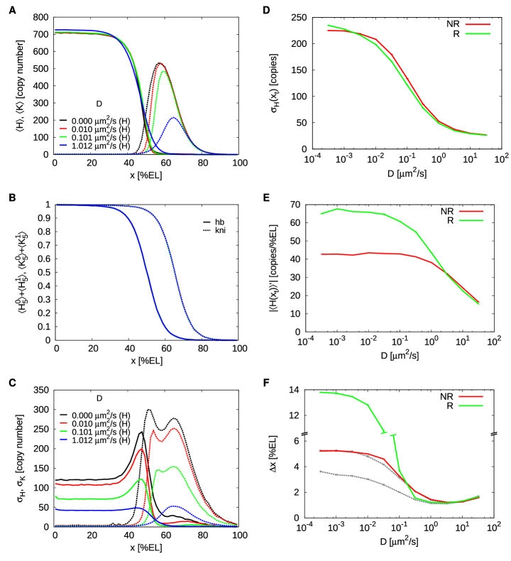
Figure S4: The effect of mutual repression in a system where both hb and kni are activated by the Bcd gradient. See following page for description.

We simulated a system in which hb and kni mutually repress each other, yet both are activated by Bcd, with kni having a lower Bcd activation threshold than hb. This generates a Hb and Kni domain, with the latter being located towards the posterior of the former (see Fig. S4 in Text S1). We systematically varied the mutual repression strength and the diffusion constant, to elucidate how mutual repression and spatial averaging sculpt stable expression patterns in this motif. Our analysis reveals that since hb and kni are both activated by the same morphogen gradient, hb should repress kni more strongly than vice versa: with equal mutual repression strengths either a spotty gap-gene expression pattern emerges in the anterior half, namely when the Hb and Kni diffusion constant are low ($D<0.1\,\mathrm{\mu m^{2}/s}$), or Kni dominates or even squeezes out Hb, namely when their diffusion constant is large. Nonetheless, for unequal mutual repression strengths and sufficiently high $D$, the repression of hb by kni does enhance the precision and the steepness of the Hb boundary, although the effect is smaller than in the two-gradient motif (Fig. S4 in Text S1). Clearly, while the one-morphogen-gradient motif cannot provide the robustness against embryo-to-embryo variations in morphogen levels that the two-morphogen-gradient motif can provide, mutual repression can enhance boundary precision also in this motif.

Discussion

Using large-scale stochastic simulations, we have examined the role of mutual repression in shaping spatial patterns of gene expression, with a specific focus on the hb-kni system. Our principal findings are that mutual repression enhances the robustness both against intra-embryonic fluctuations due to noise in gap-gene expression and embryo-to-embryo variations in morphogen levels.

To investigate the importance of mutual repression in shaping gene-expression patterns, we have systematically varied a large number of parameters: the strength of mutual repression, the diffusion constant of the gap proteins, the maximum expression level, the Hill coefficient of gap-gene activation, and the amplitude of the morphogen gradients. To elucidate how varying these parameters changes the precision of the gap-gene boundaries, we examined how they affect both the steepness of the gene-expression boundaries and the expression noise at these boundaries (see Eq. 1). The effect on the steepness is, to a good approximation, independent of the noise, and would therefore be more accessible experimentally. We find that the steepness increases with decreasing diffusion constant, but increases with increasing strength of mutual repression, maximum expression level, and Hill coefficient of gap-gene activation. Moreover, mutual repression shifts the expression boundaries apart and makes the system more robust to embryo-to-embryo variations in the morphogen levels. In contrast, the noise at the expression boundaries decreases with increasing diffusion constant, decreasing expression level, and decreasing Hill coefficient, while the dependence on the strength of mutual repression is non-monotonic, albeit not very large. The interplay between noise and steepness means that the precision of the gap-gene expression boundaries increases (i.e., $\Delta x$ decreases) with increasing expression level. The dependence of $\Delta x$ on the diffusion constant and the strength of mutual repression, on the other hand, is non-monotonic: there is an optimal diffusion constant and repression strength that maximizes precision. The effect of the Hill coefficient is conditional on the strength of mutual repression: without mutual repression, the precision slightly decreases with increasing Hill coefficient, while with mutual repression the precision increases with increasing Hill coefficient.

While mutual repression has only a weak effect on the noise in the expression levels at the gene-expression boundaries, it does markedly steepen the boundaries, especially when the diffusion constant is low. Indeed, mutual repression can enhance the precision of gene expression boundaries by steepening them. Nonetheless, even with mutual repression spatial averaging [20, 19] appears to be a prerequisite for achieving precise expression boundaries: without diffusion of the gap proteins, the width of the hb expression boundary is larger than that observed experimentally [6]. Hence, while previous mean-field analysis found diffusion not be important for setting up gene-expression patterns [28, 12], our analysis underscores the importance of diffusion in reducing copy-number fluctuations. In addition, diffusion can anneal patterning defects that might arise from the bistability induced by mutual repression. Diffusion is, indeed, a potent mechanism for reducing the effect of fluctuations, such that mean-field analyses can accurately describe mean expression profiles.

Interestingly, the minimum boundary width at the optimal diffusion constant in a system with mutual repression is not much lower than that in one without mutual repression. Yet, in the latter case the boundary width is already approximately one nuclear spacing, and there does not seem to be any need for reducing it further. However, with mutual repression, the same boundary width can be obtained at a lower diffusion constant, where the steepness of the boundaries is much higher, approximately twice as high as that without mutual repression. Our results thus predict that mutual repression allows for gap-gene expression boundaries that are both precise and steep. In fact, the width and steepness of the boundaries as prediced by our model are in accordance with those measured experimentally [11].

Our observation that mutual repression increases the steepness of gene-expression boundaries without significantly raising the noise, makes the mechanism distinct from other mechanisms for steepening gene expression boundaries, such as lowering diffusion constants [19] or increasing the cooperativity of gene activation (see Fig. S6 in Text S1). These mechanisms typically involve a trade off between steepness and noise: lowering the diffusion constant or increasing the Hill coefficient of gene activation steepens the profiles but also raises the noise in protein levels at the expression boundary. In fact, increasing the Hill coefficient (without mutual repression) decreases the precision of gene-expression boundaries. This is because increasing the Hill coefficient increases the width of the distribution of times during which the promoter is off, leading to larger promoter-state fluctuations and thereby to larger noise in gene expression (see Fig. S5 in Text S1).

Another important role of mutual repression as suggested by our simulations is to buffer against inter-embryonic variations in the morphogen levels. Houchmandzadeh et al. observed that in bcd overdosage experiments the Hb boundary does not shift as far posteriorly as predicted by the French flag model [5]. One possible explanation that has been put forward is that Bcd is inactivated in the posterior half of the embryo via a co-repressor diffusing from the posterior pole [36]. More recently, it has been proposed that gap gene cross regulation underlies the resilience of the gap-gene expression domains towards variations in the bcd gene dosage [13, 12]. Our analysis supports the latter hypothesis. In particular, our results show that when the regions in which hb and kni are acitvated by their respective morphogens overlap, the boundary positions are essentially insensitive to correlated variations in both morphogen levels, and very robust against variations of the Bcd level only, with the latter being in quantitative agreement with what has been observed experimentally [5]. Moreover, when this overlap is about 0-20% of the embryo length, mutual repression confers robustness not only against inter-embryonic variations in morphogen levels, but also intra-embryonic fluctuations such as those due to noise in gene expression.

Manu et al. found that in the kr;kni double mutant, which lacks the mutual repression between hb and kni/kr, the Hb midembryo boundary is about twice as wide as that in the wild-type embryo [13]. This could be due to a reduced robustness against embryo-to-embryo variations in morphogen levels, but it could also be a consequence of a diminished robustness against intra-embryonic fluctuations. The analysis of Manu et al. suggests the former [13, 12], and also our results are consistent with this hypothesis. However, our results also support the latter scenario: for $D\approx 0.3\,\mathrm{\mu m^{2}/s}$, the Hb boundary width in the system without mutual repression is about twice as large as that in the system with mutual repression (see Fig. 4C). Clearly, new experiments are needed to establish the importance of intra-embryonic fluctuations versus inter-embryonic variations in gene expression boundaries.

To probe the relative magnitudes of intra- vs inter-embryonic variations, one ideally would like to measure an ensemble of embryos as a function of time; one could then measure the different contributions to the noise in the quantity of interest following Eq. 5. This, however, is not always possible; staining, e.g., typically impedes performing measurements as a function of time. The question then becomes: if one measures different embryos at a given moment in time, are embryo-to-embryo variations in the mean boundary position or protein copy number (thus averaged over the circumference) due to intra-embryonic fluctuations in time or due to systematic embryo-to-embryo variations in e.g. the morphogen levels? Experiments performed on different embryos but at one time point cannot answer this question. Our analysis, however, suggests that the intra-embryonic fluctuations in the mean copy number or boundary position (i.e. averaged over $\phi$) over time are very small, and that hence embryo-to-embryo variations in the mean quantity of interest are really due to systematic embryo-to-embryo variations; these variations then correspond to $\sigma^{2}_{\mathrm{\langle\overline{G}\rangle_{\mathrm{\phi}}}}$ or $\sigma^{2}_{\mathrm{\langle\overline{x_{\mathrm{t}}}\rangle_{\mathrm{\phi}}}}$ in Eq. 5 or Eq. 7, respectively. The intra-embryonic fluctuations, $\langle\overline{\sigma^{2}_{\mathrm{G}}}\rangle_{\mathrm{e}}(x)$ or $\langle\overline{\sigma^{2}_{\mathrm{x_{\mathrm{t}}}}}\rangle_{\mathrm{e}}(x)$, can then be measured by measuring the quantity of interest, $G$ or $x_{\mathrm{t}}$, as a function of $\phi$, and averaging the resulting variance over all embryos. We expect that these observations, in particular the critical one that intra-embryonic fluctuations in the mean quantity of interest are small, also hold for non-stationary systems, although this warrants further investigation.

Our model does not include self-activation of the gap genes. Auto-activation has been reported for hb, kr and gt, but there seems to be no evidence in case of kni [56, 34]. The self-enhancement of gap genes has the potential to steepen and sharpen expression domains even more by amplifying local patterns [57, 58]. Our results suggest, however, that auto-activation is not necessary to reach the boundary steepness and precision as observed experimentally.

Our results provide a new perspective on the Waddington picture of development [59, 60]. Waddington argued that development is “canalized”, by which he meant that cells differentiate into a well-defined state, despite variations and fluctuations in the underlying biochemical processes. It has been argued that canalization is a consequence of multistability [13, 12, 28], which is the idea that cells are driven towards attractors, or basins of attraction in state space. To determine whether a given system is multistable, it is common practice to perform a stability analysis at the level of single cells or nuclei. Our results show that this approach should be used with care: diffusion of proteins between cells or nuclei within the organism can qualitatively change the energy landscape; specifically, a cell that is truly bistable without diffusion might be monostable with diffusion. Indeed, our results highlight that a stability analysis may have to be performed not at the single cell level, but rather at the tissue level, taking the diffusion of proteins between cells into account.

Finally, while our results have shown that mutual repression can stabilize expression patterns of genes that are activated by morphogen gradients, one may wonder whether it is meaningful to ask the converse question: do morphogen gradients enhance the stability of expression domains of genes that mutually repress each other? This question presupposes that stable gene expression patterns can be generated without morphogen gradients. Although it was shown that confined (though aberrant) gap gene patterns form in the absence of Bcd [61, 62, 63] and that Hb can partly substitute missing Bcd in anterior embryo patterning[64], it is not at all obvious how precise domain positioning could succeed in such a scenario. In particular, one might expect that with mutual repression only, thus without morphogen gradients, there is no force that pins the expression boundaries. Our results for the large overlapping morphogen-activation domains, with $A=8$, illustrate this problem: in the overlap region, both hb and kni are essentially fully activated by their respective morphogens, as a result of which the morphogen gradients cannot determine the positions of the gap-gene boundaries within this region; indeed, mutual repression has to pin the expression boundaries of hb and kni. Yet, our results show that in this case the positions of the hb and kni expression boundaries exhibit large and slow fluctuations, suggesting that mutual repression alone cannot pin expression boundaries. Interestingly, however, with $A=4$, the region in which both genes are activated is still quite large, about 50% of the embryo, and yet even though the underlying energy landscape is flat in this region, the interfaces do consistently move towards the middle of the embryo, due to diffusive influx of Hb and Kni from the polar regions. It is tempting to speculate that mutual repression and diffusion can maintain stable expression patterns, while morphogen gradients are needed to set up the patterns, e.g. by breaking the symmetry between the possible patterns that can be formed with mutual repression only.

Materials and Methods

In the following we describe details of our parameter choice and sampling technique. To unravel the mechanisms by which mutual repression shapes gene-expression patterns, it is useful to take the Cad-Kni-system to be a symmetric copy of the Bcd-Hb-system. Cad thus inherits its parameters from Bcd and Kni from Hb, if not otherwise stated. Table S2 in Text S1 gives an overview of our standard parameter values. Data from experiments was used whenever possible. When it was unavailable we made reasonable estimates.

Binding rates are diffusion limited. We assume all promoter binding rates to be diffusion limited and calculate them via $k_{\mathrm{on}}^{\rm X}=4\pi\alpha D_{\mathrm{X}}/V$. Here $\alpha=10~{}\,\mathrm{nm}$ is the typical size of a binding site, $D_{\mathrm{X}}$ is the intranuclear diffusion constant of species $X$ and $V=143.8~{}\mu{\rm m}^{3}$ is the nuclear volume. The precise values of $D_{\mathrm{X}}$ for the different species in our system are not known. Gregor et al. have shown experimentally that the nuclear concentration of Bcd is in permanent and rapid dynamic equilibrium with the cytoplasm [7], suggesting that nuclear and cytoplasmic diffusion constants can be taken for equal. They have found $D_{\mathrm{Bcd}}\simeq 0.32~{}\,\mathrm{\mu m^{2}/s}$ by FRAP measurements. This value has been subject to controversy because it is too low to establish the gradient before nuclear cycle 10 ($\simeq 90~{}\,\mathrm{min}$) by diffusion and degradation only, prompting alternative gradient formation models [65, 66, 67, 68, 69, 70]. A more recent study revisited the problem experimentally via FCS, yielding significantly higher values for $D_{\mathrm{Bcd}}$ up to $10~{}\,\mathrm{\mu m^{2}/s}$ with a lower limit of $1~{}\,\mathrm{\mu m^{2}/s}$ [71]. We therefore have chosen a 10x higher value of $D_{\mathrm{Bcd}}=D_{\mathrm{Cad}}\equiv D_{\mathrm{A}}=3.2~{}\,\mathrm{\mu m^{2}/s}$ as compared to the earlier choice in [19]. For simplicity, this value is taken for all binding reactions occuring in our model, except for the dimerization reaction rate $k_{\mathrm{on}}^{\rm D}$, which is taken to be higher by a factor of 2 to account for the fact that both reaction partners diffuse freely.

To model cooperative activation of hb and kni by their respective morphogens, the morphogen-promoter dissociation rate is given by $k_{\mathrm{off,n}}^{\rm A}=a/b^{n}/{\rm s}$, where $n$ is the number of morphogen molecules that are bound to the promoter; for our standard cooperativity $n_{\mathrm{max}}=5$ the values of $a=410$ and $b=6$ have been chosen such that the threshold concentration for promoter activation (in the absence of repression) equals the observed average number of morphogen molecules at midembryo (when $A=1$, see below). $n_{\mathrm{max}}$ is varied in some simulations; we describe in Text S1 how $a$ and $b$ are chosen in these cases. The promoter unbinding rate of hb and kni (the repressor-promoter unbinding rate) $k_{\mathrm{off}}^{\rm R}$ is a parameter that we vary systematically. To study the potential role of bistability we decided to set $k_{\mathrm{off}}^{\rm R}$ to a value which ensures bistable behavior when both hb and kni are fully activated by their respective morphogens (meaning that all five binding morphogen-binding sites on the promoter are occupied). This requires tight repression, yielding dissociation constants $\sim 10^{-2}~{}\,\mathrm{nM}$ (but see also below). The dimer dissociation rate is set to be $k_{\mathrm{off}}^{\rm D}=k_{\mathrm{on}}^{\rm D}/V$, which is motivated by the choice for the toggle switch models studied in [26, 27] and [49], and asserts that at any moment in time the majority of the gap proteins is dimerized. This is a precondition for bistability in the mean-field limit [24, 26, 27].

The parameters of the exponential morphogen gradients are chosen such that the number of morphogen molecules at midembryo and the decay length of the gradient are close to the experimentally observed values for Bcd, 690 and $\lambda=119.5~{}\,\mathrm{\mu m}$, respectively [6].

Production and degradation dynamics. The copy numbers of both monomers and dimers and the effective gap gene degradation rate $\mu_{\mathrm{eff}}$ depend in a nontrivial manner on production, degradation and dimerization rates. However, for constant production rate $\beta$, without diffusion and neglecting promoter dynamics, an analytical estimate for the monomer and dimer copy numbers can be obtained from steady state solutions of the rate equations (see Text S1). Based on this we have made a choice for $\beta$ and the monomeric ($\mu_{\mathrm{M}}$) and dimeric ($\mu_{\mathrm{D}}$) decay rates that leads to reasonable copy numbers and $\mu_{\mathrm{eff}}$ (see Table S2 in Text S1). The latter is defined as the mean of $\mu_{\mathrm{M}}$ and $\mu_{\mathrm{D}}$ weighted by the species fractions. $\mu_{\mathrm{M}}$ and $\mu_{\mathrm{D}}$ are set such that $\mu_{\mathrm{eff}}\simeq 4.34\cdot 10^{-3}~{}\,\mathrm{1/s}$, which corresponds to an effective protein lifetime of $\sim 4~{}\,\mathrm{min}$. This is close to values used earlier [36, 19] and allows for the rapid establishment of the protein profiles observed in experiments. The dimers have a substantially lower degradation rate than monomers, which enhances bistability [72]. The lower decay rate of the dimers may be attributed to a stabilizing effect of oligomerization (cooperative stability) [72].

Free parameters. One of the key parameters that we vary systematically is the internuclear gap gene diffusion constant $D$, which defines a nuclear exchange rate $k_{\mathrm{ex}}=4D/\ell^{2}$ ($\ell$ = internuclear distance). To study the effect of embryo-to-embryo variations in the morphogen levels, the latter are scaled globally by a dosage factor $A$. We considered two scenarios: scaling both gradients by the same $A$ (“correlated variations”) or scaling the Bcd gradient only (“uncorrelated variations”). To test how strongly the assumption of strong repressor-promoter binding affects our results, we also varied the repressor-promoter dissociation rate $k_{\mathrm{off}}^{\rm R}$. Moreover, to study the dependence of our results on the gap-gene copy numbers, we also increased the protein production rate $\beta$. These simulations are much more computationally demanding; therefore we limited ourselves to simulations with $\beta=2\beta_{\mathrm{0}}$ and $\beta=4\beta_{\mathrm{0}}$ where $\beta_{\mathrm{0}}$ is our baseline value. Finally we also studied a system where both gap genes are activated by the same gradient (Bcd), varying both the diffusion constant $D$ and the Kni repressor off-rate $k_{\mathrm{off}}^{\rm R,Kni}$, while keeping $k_{\mathrm{off}}^{\rm R,Hb}$ at the standard value.

Algorithmic details. All simulations are split into a relaxation and a measurement run. During the relaxation run we propagate the system towards the steady state without data collection. To reach steady state, as a standard we run $1\cdot 10^{9}-3\cdot 10^{9}$ Gillespie steps (ca. $2\cdot 10^{5}-7\cdot 10^{5}$ updates per nucleus). The measurement run is performed with twice the number of steps ($2\cdot 10^{9}-6\cdot 10^{9}$). The simulations are started from exponential morphogen gradients and step profiles of the gap proteins; however, we verified that the final result was independent of the precise initial condition, and that the system reached steady state after the equilibration run. The results for $A=4$ (Fig. 7) form, however, an exception: here it was impossible to obtain a reliable error bar, because of the weak pinning force on the hb and kni expression boundaries.

In steady state, we record for each row of nuclei and with a measurement interval of $\tau_{\mathrm{m}}=100~{}\,\mathrm{s}$ the Hb boundary position $x_{\mathrm{t}}$, i.e. the position where $H$ drops to half of the average steady-state value measured at its plateau close to the anterior pole, which in our simulations is equal to the maximum average total Hb level $\langle H\rangle_{\mathrm{max}}$. From the corresponding histogram we obtain the boundary width $\Delta x$ by computing the standard deviation. Additionally, after runtime we calculate an approximation for $\Delta x$ from the standard deviation of $H$ divided by the slope of the averaged $H$ profile, both quantities taken at $x_{\mathrm{t}}$, see Eq. 1 [6, 35, 19]. Further details of boundary measurement are described in Text S1.

Error bars for a given quantity are estimated from the standard deviation among $N_{\mathrm{B}}=10$ block averages (block length $6\cdot 10^{8}$) divided by $\sqrt{N_{\mathrm{B}}-1}$, following the procedure described in [73]. We verified that estimates with smaller and larger block sizes yield similar estimates for a representative set of simulations.

SUPPORTING TEXT S1

1 Methodic details

1.1 Measurement of the boundary width

By default we determine the boundary width in the following two ways:

Let $c^{\mathrm{m}}_{\mathrm{n,s}}$ be the copy number of species $s$ in a nucleus with angular index $m<N_{\mathrm{\phi}}$ and axial index $n<N_{\mathrm{x}}$, where $N_{\mathrm{\phi}}$ is the number of rows around the circumference of the cylinder, and $N_{\mathrm{x}}$ is the number of colums in the axial direction along the AP axis. To compute the boundary width of the expression domain of a gap protein $s$, we compute for each row $m$ $T^{\mathrm{m}}_{\mathrm{n,s}}=(c^{\mathrm{m}}_{\mathrm{n,s}}-\theta_{\mathrm{s}})\cdot(c^{\mathrm{m}}_{\mathrm{n+1,s}}-\theta_{\mathrm{s}})$ as a function of $n$, where $\theta_{\mathrm{s}}$ is half the copy number expected at full activation. A boundary position $x^{\mathrm{m}}_{\mathrm{t}}=x^{\mathrm{m}}(n_{\mathrm{t}}+\frac{1}{2})$ is defined as the position (nucleus) where $T^{\mathrm{m}}_{\mathrm{n_{\mathrm{t}},s}}<0$. The values of $x^{\mathrm{m}}_{\mathrm{t}}$ are recorded in a histogram; here, the positions for the different rows $m$ are put in the same histogram. The histogram is normalized at the end of the simulation, and the boundary width $\Delta x$ is calculated as the standard deviation of this histogram.

Secondly, at the end of the simulation, the slope of the average, $\langle H(x_{\mathrm{t}})\rangle^{\prime}$, and the standard deviation of the total Hb copy number $\sigma_{\mathrm{H}}(x_{\mathrm{t}})$ at the Hb boundary position $x_{\mathrm{t}}$ are calculated from the time- and $\phi$-averaged profiles. From this, an approximation for the boundary width given by $\Delta x\approx\frac{\sigma(x_{\mathrm{t}})}{|\langle H(x_{\mathrm{t}})\rangle^{\prime}|}$ is obtained, following [35, 6, 19]. To this end, first $x_{\mathrm{t}}$ is determined in the same way as in the runtime measurements, only now working on the (both time- and circumference-) averaged profile. We describe in the following section how the steepness $\langle H(x_{\mathrm{t}})\rangle^{\prime}$ is measured.

1.2 Measurement of the profile steepness

In our discrete system the measurement of a local derivative at the boundary position $x_{\mathrm{t}}$ is a process prone to even small stochastic variations if a naive measurement technique is chosen. If the average boundary position $x_{\mathrm{t}}$ for a set of different samples with identical initial conditions always is in between two particular nuclear positions $x(n_{\mathrm{0}})$ and $x(n_{\mathrm{0}}+1)$, then using linear differences to determine the steepness $\langle H(x_{\mathrm{t}})\rangle^{\prime}$ at the boundary position may give a reasonable estimate. If, however, $x_{\mathrm{t}}$ fluctuates around a particular nuclear position $x(n_{\mathrm{0}})$ among different samples and $\langle H(x(n_{\mathrm{0}}-1))\rangle-\langle H(x(n_{\mathrm{0}}))\rangle$ significantly differs from $\langle H(x(n_{\mathrm{0}}))\rangle-\langle H(x(n_{\mathrm{0}}+1))\rangle$, the linear differences method will produce a large error bar and also markedly affect the mean of $x_{\mathrm{t}}$ among these samples. As a result both the measured steepness and the quality of that measurement for a given set of parameters depends on whether $x_{\mathrm{t}}$ accidently happens to predominantly vary in the interval between the same nuclear positions or not. To overcome this illness we measure the boundary steepness from the average protein profile by a two-step polynomial fitting procedure: First we fit a polynomial of 3rd degree to a region of the data around $x_{\mathrm{t}}$ that contains at least four points (nuclei). The derivative of the polynomial at $x_{\mathrm{t}}$ gives an initial estimate of the boundary slope, which we use this to calculate the approximative x-interval over which the profile falls from maximal to minimial expression level. If the latter is larger than the original fitting range (which usually is the case) we repeat the fitting on the enlarged interval. Since the profiles to a good approximation are sigmoidal functions this improves the quality of the fit. The measured boundary slope then is defined as the derivative of the polynomial function at $x_{\mathrm{t}}$ after the second fitting.

1.3 Number of cortical nuclei at cell cycle 14

The development of the Drosophila embryonic syncytium starts with a single nucleus. The first 9 nuclear divisions happen in the yolk. During cell cycles 7 to 10 a migration of the nuclei towards the cortex can be observed. However, approximately 200 polyploid nuclei stay behind in the yolk and stop dividing after their 10th cycle [38]. This quiescence persists during subsequent cell cycles, including cycle 14. As an effect of this, the number of nuclei at the cortex in cycle 14 is considerably lower than $2^{13}=8192$. An estimate of the reduced number of cortical nuclei is given by:

$$N_{\mathrm{cortex}}\simeq(2^{9}-200)\cdot 2^{4}=4992$$ (8)

This number indeed is closer to $2^{12}$ than to $2^{13}$. Note that in our model the precise number of nuclei does not matter, rather it is the distance between the nuclear compartments and the diffusion correlation length that impact on the results. Our values for both the internuclear distance and the nuclear diameter correspond to the experimental values reported by Gregor et al. [6, 7].

1.4 Predicted copy numbers and effective protein lifetime

Our main observables are the total copy numbers of Hb and Kni, defined as follows:

$$H\equiv c^{\mathrm{m}}_{\mathrm{n,H}}=c^{\mathrm{m}}_{\mathrm{n,H_{\mathrm{M}}}}+2c^{\mathrm{m}}_{\mathrm{n,H_{\mathrm{D}}}}+2\sum_{\mathrm{j=0}}^{5}c^{\mathrm{m}}_{\mathrm{n,K^{1}_{\mathrm{j}}}}$$

$$K\equiv c^{\mathrm{m}}_{\mathrm{n,K}}=c^{\mathrm{m}}_{\mathrm{n,K_{\mathrm{M}}}}+2c^{\mathrm{m}}_{\mathrm{n,K_{\mathrm{D}}}}+2\sum_{\mathrm{j=0}}^{5}c^{\mathrm{m}}_{\mathrm{n,H^{1}_{\mathrm{j}}}}$$ (9)

Here, for $G\in\{H,K\}$, $c^{\mathrm{m}}_{\mathrm{n,G^{1}_{\mathrm{j}}}}=1$ if the promoter of species G is binding $j$ morphogen molecules and one (repressing) gap dimer; evidently, at any given moment in time $c^{\mathrm{m}}_{\mathrm{n,G_{\mathrm{j}}^{1}}}$ can be equal to one for only one $j\in\{0..5\}$.

The ratio between the number of monomeric and the number of dimeric proteins is a nontrivial function of the monomer production rate, the monomer and dimer degradation rates and the parameters that determine the dimerization and dedimerization reactions. To obtain an estimate for the expected copy numbers of monomers and dimers of gene $g$ we solved the mean-field rate equations for a simplified model which comprises monomer production, (de)dimerization and monomer and dimer degradation only, i.e. in which promoter state fluctuations and diffusion are neglected, in the steady state. We assume here that stochastic monomer production events can be accounted for by an effective mean-field production rate $\langle\beta\rangle=\beta\langle H_{\mathrm{5}}^{0}\rangle$ for Hb and similarly for Kni, which depends on promoter (un)binding parameters and the particular morphogen and repressor levels. This yields the following prediction for the copy number of monomers ($G_{\mathrm{M,\langle\beta\rangle}}$) and dimers ($G_{\mathrm{D,\langle\beta\rangle}}$):

$$G_{\mathrm{M,\langle\beta\rangle}} =\frac{1}{4k^{\mathrm{D}}_{\mathrm{on}}\mu_{\mathrm{D}}}\Bigg{\{}2k^{\mathrm{D}}_{\mathrm{on}}\mu_{\mathrm{D}}-k^{\mathrm{D}}_{\mathrm{off}}\mu_{\mathrm{M}}-\mu_{\mathrm{M}}\mu_{\mathrm{D}}$$

$$\hskip 54.06006pt+\sqrt{8\langle\beta\rangle k^{\mathrm{D}}_{\mathrm{on}}\mu_{\mathrm{D}}\left(k^{\mathrm{D}}_{\mathrm{off}}+\mu_{\mathrm{D}}\right)+\left[\mu_{\mathrm{M}}\left(k^{\mathrm{D}}_{\mathrm{off}}+\mu_{\mathrm{D}}\right)-2k^{\mathrm{D}}_{\mathrm{on}}\mu_{\mathrm{D}}\right]^{2}}\Bigg{\}}$$

$$G_{\mathrm{D,\langle\beta\rangle}} =\frac{1}{8k^{\mathrm{D}}_{\mathrm{on}}\mu_{\mathrm{D}}^{2}}\Bigg{\{}k^{\mathrm{D}}_{\mathrm{off}}\mu_{\mathrm{M}}^{2}+\mu_{\mathrm{D}}\left[4\langle\beta\rangle k^{\mathrm{D}}_{\mathrm{on}}+\mu_{\mathrm{M}}\left(\mu_{\mathrm{M}}-2k^{\mathrm{D}}_{\mathrm{on}}\right)\right]$$

$$\hskip 54.06006pt-\mu_{\mathrm{M}}\sqrt{8\langle\beta\rangle k^{\mathrm{D}}_{\mathrm{on}}\mu_{\mathrm{D}}\left(k^{\mathrm{D}}_{\mathrm{off}}+\mu_{\mathrm{D}}\right)+\left[\mu_{\mathrm{M}}\left(k^{\mathrm{D}}_{\mathrm{off}}+\mu_{\mathrm{D}}\right)-2k^{\mathrm{D}}_{\mathrm{on}}\mu_{\mathrm{D}}\right]^{2}}\Bigg{\}}$$ (10)

Here $\mu_{\mathrm{M}}$ ($\mu_{\mathrm{D}}$) is the monomeric (dimeric) degradation rate and $k_{\mathrm{on}}^{\rm D}$ ($k_{\mathrm{off}}^{D}$) are the dimerization forward (backward) rates, respectively. From this we calculate the total expected copy number $G_{\mathrm{\langle\beta\rangle}}:=2G_{\mathrm{D,\langle\beta\rangle}}+G_{\mathrm{M,\langle\beta\rangle}}$ at effective production rate $\langle\beta\rangle$. In particular in the full-activation case, i.e. when the probability to be fully activated and unrepressed $\langle G^{\mathrm{0}}_{\mathrm{5}}\rangle\approx 1$ and therefore $\langle\beta\rangle\approx\beta$, the above estimates correspond to average values from our simulations very well.

We define the effective degradation as $\mu_{\mathrm{eff}}=\mu_{\mathrm{eff}}(G_{\mathrm{M}},G_{\mathrm{D}})=\frac{1}{G_{\mathrm{M}}+2G_{\mathrm{D}}}\left(\mu_{\mathrm{M}}G_{\mathrm{M}}+2\mu_{\mathrm{D}}G_{\mathrm{D}}\right)$. Our standard values result in $\mu_{\mathrm{eff}}\approx 4.34\cdot 10^{-3}\,\mathrm{/s}$ with $G_{\mathrm{M}}=G_{\mathrm{M,\beta}}$ and $G_{\mathrm{D}}=G_{\mathrm{D,\beta}}$.

2 Additional analysis

2.1 Poissonian limit with dimerization

In [19], it was shown that, when $D\to\infty$, the variance in the protein concentration becomes equal to the mean concentration: diffusion washes out bursts in gene expression, thus reducing the non-Poissonian part of the noise. However, in that model the proteins do not dimerize, in contrast to our model. With dimerization, a different limit for the variance in the total protein concentration is approached as $D\to\infty$. To derive this limit, first note that the total protein copy number $G$ of a protein G is $G\approx 2G_{\mathrm{D}}+G_{\mathrm{M}}$. Assuming that $\langle G_{\mathrm{D}}G_{\mathrm{M}}\rangle\approx\langle G_{\mathrm{D}}\rangle\langle G_{\mathrm{M}}\rangle$ (our simulations indicate that this approximation is very accurate), we find that the variance $\sigma^{2}_{\mathrm{G}}$ in $G$ is:

$$\sigma^{2}_{\mathrm{G}}\approx 4\sigma^{2}_{\mathrm{G_{\mathrm{D}}}}+\sigma^{2}_{\mathrm{G_{\mathrm{M}}}},$$ (11)

where $\sigma^{2}_{\mathrm{G_{\mathrm{D}}}}$ is the variance in the dimer level $G_{\mathrm{D}}$ and $\sigma^{2}_{\mathrm{G_{\mathrm{M}}}}$ is the variance in the monomer level $G_{\mathrm{M}}$. Both monomers and dimers are subject to spatial averaging, and therefore their variances can be written in the form [19]:

$$\sigma^{2}_{\mathrm{G_{\mathrm{M}}}}=G_{\mathrm{M}}+\frac{1}{N}\left(\sigma^{2}_{\mathrm{0,G_{\mathrm{M}}}}-G_{\mathrm{M}}\right)$$

$$\sigma^{2}_{\mathrm{G_{\mathrm{D}}}}=G_{\mathrm{D}}+\frac{1}{N}\left(\sigma^{2}_{\mathrm{0,G_{\mathrm{D}}}}-G_{\mathrm{D}}\right)$$ (12)

Here $N$ is the number of nuclei contributing to the averaging, which is proportional to $D$, and $\sigma^{2}_{\mathrm{0,G_{\mathrm{M/D}}}}$ is the variance in the monomer and dimer levels in the absence of diffusion, respectively. The part preceded by $1/N$ represents the variance that can be reduced by spatial averaging. Plugging these expressions into the previous and using $G=2G_{\mathrm{D}}+G_{\mathrm{M}}$ we arrive at:

$$\sigma^{2}_{\mathrm{G}} =4G_{\mathrm{D}}+G_{\mathrm{M}}+\frac{1}{N}\left[4\sigma^{2}_{\mathrm{0,G_{\mathrm{D}}}}+\sigma^{2}_{\mathrm{0,G_{\mathrm{M}}}}-4G_{\mathrm{D}}-G_{\mathrm{M}}\right]$$

$$=\left(1+\frac{2G_{\mathrm{D}}}{G}\right)G+\frac{1}{N}\left[\sigma^{2}_{\mathrm{0,G}}-\left(1+\frac{2G_{\mathrm{D}}}{G}\right)G\right]$$

$$=:\left(1+f_{\mathrm{D}}\right)G+\frac{1}{N}\left[\sigma^{2}_{\mathrm{0,G}}-\left(1+f_{\mathrm{D}}\right)G\right]$$ (13)

Note that $N$ is the same for both monomers and dimers because their diffusion constant does not differ in our model. Evidently, the lower bound for $\sigma_{\mathrm{G}}$ in the limit $N\rightarrow\infty$ is not $\sqrt{G}$ any more, but given by $\sqrt{\left(1+f_{\mathrm{D}}\right)G}$, where $f_{\mathrm{D}}$ is the fraction of proteins in the dimer state with respect to the total protein number (implying $f_{\mathrm{D}}\leq 1$). This is indeed what we observe in our data for $\sigma_{\mathrm{G}}$. In our simulations the equilibrium is strongly shifted towards the dimerized state, so that $f_{\mathrm{D}}\approx 0.97$. We can understand the limit $N,D\rightarrow\infty$ intuitively by noting that in this limit there is no noise in the nuclear protein concentration due to the stochastic production and decay of molecules in each of the nuclei—this is because the synthesized molecules are immediately donated to a reservoir that is infinitely large; instead, there is only noise in the nuclear protein concentration due to the sampling of molecules from this reservoir, which obeys Poissonian statistics: $\sigma^{2}_{\mathrm{G_{\mathrm{M}}}}=G_{\mathrm{M}}$ and $\sigma^{2}_{\mathrm{G_{\mathrm{D}}}}=G_{\mathrm{D}}$. This yields, for $N,D\rightarrow\infty$, $\sigma^{2}_{\mathrm{G}}=4\sigma^{2}_{\mathrm{G_{\mathrm{D}}}}+\sigma^{2}_{\mathrm{G_{\mathrm{M}}}}=4G_{\mathrm{D}}+G_{\mathrm{M}}=(1+f_{\mathrm{D}})G$.

2.2 Bifurcation analysis

In order to predict the regions in which bistability can be expected for different amplitudes $A$ of the morphogen gradients we performed a deterministic mean-field bifurcation analysis for a simplified 1-dimensional version of our model of mutual repression between hb and kni. The analysis is based on the following two equations describing the change of the mean-field total copy number of Hb ($H(x)$) and Kni ($K(x)$) at position $x$:

$$\partial_{\mathrm{t}}H(x) =\beta_{\mathrm{H}}(x)\frac{K_{\mathrm{R}}^{2}}{K_{\mathrm{R}}^{2}+\left[f_{\mathrm{D}}K(x)\right]^{2}}-\mu_{\mathrm{H}}H(x)$$ (14)

$$\partial_{\mathrm{t}}K(x) =\beta_{\mathrm{K}}(x)\frac{K_{\mathrm{R}}^{2}}{K_{\mathrm{R}}^{2}+\left[f_{\mathrm{D}}H(x)\right]^{2}}-\mu_{\mathrm{K}}K(x)$$ (15)

Here $\beta_{\mathrm{H}}$ and $\beta_{\mathrm{K}}$ represent the protein synthesis rates, $\mu_{\mathrm{H}}$ and $\mu_{\mathrm{K}}$ the corresponding (effective) degradation rates, $K_{\mathrm{R}}$ is the dissociation constant of cooperative repressor binding to the promoter and $f_{\mathrm{D}}$ is the fraction of proteins in the dimerized state. Note that, since the intermediate step of dimerization is neglected here, we have to take $K_{\mathrm{R}}=\sqrt{k^{R}_{\mathrm{off}}/k^{R}_{\mathrm{on}}}$ if $k^{R}_{\mathrm{on}}$ and $k^{R}_{\mathrm{off}}$ are the binding rates of the dimers. To facilitate calculations we make two further simplifying assumptions here:

1. We neglect activation dynamics and resulting promoter state fluctuations, i.e. we assume that certain constant levels of the activators at position $x$ lead to average constant production rates $\beta_{\mathrm{H}}=\beta([Bcd](x))$ and $\beta_{\mathrm{K}}=\beta([Cad](x))$, respectively. In our standard case $\beta([Act](x))=[Act]^{5}(x)/([Act]^{5}(x)+690^{5})$ for both $[Act]=[Bcd]$ and $[Act]=[Cad]$.

2. In our simulations we have different degradation rates for monomers and dimers so that the effective total degradation rate depends on the monomer-to-dimer ratio, which in turn varies with the total copy number (see section 1.4). Thus, in principle, also $f_{\mathrm{D}}$ and $\mu_{\mathrm{H}}$ and $\mu_{\mathrm{K}}$ are functions of $x$, or the corresponding activator levels. Since this introduces further nonlinearities into the above equations and complicates their solution, we substitute the degradation rates $\mu_{\mathrm{H}}$ and $\mu_{\mathrm{K}}$ by a constant value $\mu_{\mathrm{eff}}$, which is the effective degradation rate for the maximal expression level (full activation). Also for $f_{\mathrm{D}}$ we take the constant value for full activation, $f_{\mathrm{D}}\simeq 0.97$, which reflects that the dimerization equilibrium in our simulations is strongly shifted towards the dimerized state. The predictions concerning the bifurcation behavior only change marginally if $\mu_{\mathrm{eff}}$ and $f_{\mathrm{D}}$ values for lower expression levels are used.

For each position $x$ with local activator levels corresponding to the ones in the simulations we calculated fixed point solutions for the copy number pair $(H(x),K(x))$ starting from the steady-state assumption $\partial_{\mathrm{t}}(H(x),K(x))=(0,0)$. The stability of the fixed points was determined starting from the Jacobian for the above ODE system:

$$J(H,K)=\left(\begin{array}[]{cc}\partial_{\mathrm{H}}\left[\partial_{\mathrm{t}}H\right]&\partial_{\mathrm{K}}\left[\partial_{\mathrm{t}}H\right]\\ \partial_{\mathrm{H}}\left[\partial_{\mathrm{t}}K\right]&\partial_{\mathrm{K}}\left[\partial_{\mathrm{t}}K\right]\\ \end{array}\right)\\$$ (16)

Within the relevant parameter regime we obtained fixed points with either two negative eigenvalues (i.e. stable fixed points) or one positive and one negative eigenvalue (i.e. saddle points). The determinant therefore completely characterizes the stability of the fixed points. If $\det J(H_{\mathrm{0}},K_{\mathrm{0}})<0$, then $(H_{\mathrm{0}},K_{\mathrm{0}})$ is a saddle point. Otherwise it is stable.

Fig. S1 shows the fixed point solutions for Hb and Kni as a function of $x$ for different activator amplitudes $A$. Stable solutions are drawn with solid, unstable solutions with dashed lines. Depending on the $A$ value, the system displays a saddle node bifurcation at a point towards the anterior (Hb) or posterior (Kni) from midembryo. Within the region confined by the bifurcation points two stable and one unstable fixed points exist for each gene, implying bistability. The region clearly widens for increasing $A$ and spans almost the whole embryo length for $A=8$. Our deterministic analysis therefore predicts the enlargement of the region of bistability as observed in our single nucleus simulations.

2.3 Estimation of switching times

To quantify the swiching times in the presence of bistability we performed simulations of isolated single nuclei featuring the same set of reactions and parameters as in the full scale simulation. To obtain estimates of switching times at different positions $x$ along the AP axis we set the levels of Bcd and Cad in the given nucleus equal to the ones at $x$ in the space-resolved simulations. The switching time was estimated by calculating from long time trajectories of the total Hb and Kni copy numbers the relaxation time $t_{\mathrm{s}}$ of the average correlation function

$$\langle C(t)\rangle_{\mathrm{t_{\mathrm{0}}}}\equiv\frac{\langle I_{\mathrm{H}}(t_{\mathrm{0}})I_{\mathrm{K}}(t)\rangle_{\mathrm{t_{\mathrm{0}}}}}{\langle I_{\mathrm{H}}(t_{\mathrm{0}})\rangle_{\mathrm{t_{\mathrm{0}}}}}$$ (17)

where $I_{\mathrm{H}}$ ($I_{\mathrm{K}}$) are indicator functions which are one if the difference in the total gap gene copy numbers $\Delta N=H-K$ is above (below) a certain threshold $\Theta_{\mathrm{N}}$ ($-\Theta_{\mathrm{N}}$). $\Theta_{\mathrm{N}}$ thus defines the regions within which the switch is considered to have switched to the Hb–high or Kni–high states, respectively, and serves to separate the stable attractor states from the transition region. We found that $\Theta_{\mathrm{N}}=200$ is a reasonable choice for our set of parameters.

We determined the switching times from one long sample for different positions $x$ and different activator amplitudes $A$ and find that $t_{\mathrm{s}}$ is very similar within the double-activated bistable regions for high $A$. To obtain an error estimate we additionally calculated block averages of estimated switching times among 10 long samples for various $A$ at midembryo ($x=L/2$). Table S1 shows our results from the latter procedure.

Table S1: Switching times at midembryo for different activator levels.

Activator amplitude $A$	Switching time $t_{\mathrm{s}}[s]$
(1)	(6343.7 $\pm$ 17.2)
2	20302.5 $\pm$ 74.5
4	20957.3 $\pm$ 54.9
8	20994.7 $\pm$ 67.2

Note that for $A=1$ the system is not truly bistable yet because for $A=1$ we have half-activation at midembryo and due to the lack of diffusion large promoter-state fluctuations dominate over long-time switching potentially induced by mutual repression. Consequently, the given number does not reflect a switching time. We cite it here for completeness, however.

2.4 Analysis of statistical properties of the boundary

Our measures for both the boundary steepness and the variance of the boundary position are based on averages over both the time and the circumference of the embryo which were calculated during runtime. While the double-averaging procedure limits the amount of data that must be stored and facilitates rapid acquisition of good statistics, it also discards information about the microscopic properties of the boundary at a given time instance. Based on the average data it is impossible to determine whether the blurring of the boundary quantified by $\Delta x$ is due to concerted stochastic movements of a steep and rather homogeneous instantaneous boundary or simply due to stochastic fluctuations of the boundary position in each nuclear row around a well-defined constant mean boundary position (or due to both). In the latter case the boundary will be rough at each given time instance, i.e. the time average of the boundary position variance in the cicumferential direction will be large, but the time variance of its circumferential mean will be negligible. The opposite will be the case in the other extreme. These quantities therefore can be used to distinguish the two hypothetical situations. The overall boundary width in both cases is given by the sum:

$$\Delta x^{2} =\overline{\sigma^{2}_{\mathrm{x_{\mathrm{t}}(\phi)}}}+\sigma^{2}_{\mathrm{\langle x_{\mathrm{t}}\rangle_{\mathrm{\phi}}(t)}}$$ (18)

Here $\langle\dots\rangle_{\mathrm{\phi}}$ denotes the average over the circumference, while the bar denotes the time average. An identical variance decomposition can be made for the fluctuations of the Hb copy number at any position $x$ along the AP axis. Similarly, comparing the average of the profile steepness for a particular nuclear row and time instance to the steepness of the time- and circumference average of the copy number reveals whether the steepness of the average profile is due to concerted movements of similarly shallow instantaneous profiles or due to unconcerted fluctuations of steep instantaneous profiles.

In order to determine which of the portrayed blurring mechanisms is dominant in our system we performed the described variance decomposition for a set of 100 instantaneous outputs of the fully resolved 2D system in steady state, i.e. for 6400 different total Hb copy number profiles along the AP axis, for both the variances at the boundary and for the steepness at the boundary and for both the system with and without mutual repression. We focused on our standard parameter set (see Table S2) and a range of gap protein diffusion constants $D$.

2.4.1 At each time instance the boundary is rather rough

Fig. S2 shows for the systems with (Fig. S2A and C) and without (Fig. S2B and D) mutual repression the variance decomposition for the variance of the Hb copy number at the boundary (Fig. S2A and B) and for the variance of the boundary position $x_{\mathrm{t}}$ (Fig. S2C and D) as a function of the Hb protein diffusion constant $D$. As a control we compare the total variances calculated from the instantaneous profiles to the variances accumulated during runtime and, in case of $\Delta x$, to the value obtained from the approximation $\Delta x=\sigma_{\mathrm{H}}(x_{\mathrm{t}})/|\langle H(x_{\mathrm{t}})\rangle^{\prime}|$ (note that here $\langle\dots\rangle$ is the average over both time and $\phi$). We see a good agreement between these quantities. The plots reveal that both for $\sigma_{\mathrm{H}}(x_{\mathrm{t}})$ and $\Delta x$ the variance over the circumference at a fixed time is by far the dominant contribution to the overall variance. This implies that in our system the boundary is indeed very rough at each time point and that concerted boundary movements do not occur.

2.4.2 At each time instance the profiles are slightly steeper than their average

The calculation of the variance decomposition is less straightforward for the slope. In particular for low $D$, when spatial averaging is still inefficient, the instantaneous profiles are very ragged and the boundary threshold value typically is crossed at multiple positions along the AP axis. This makes it impossible to uniquely define an instantaneous boundary position as required to calculate the instantaneous boundary slope. In order to perform the analysis at least on a subset of the data we introduced a protocol which only takes into account instantaneous profiles with a single boundary crossing, rejecting all other profiles. For low $D$, however, the rejection rates rise above $90\%$. We therefore decided to smoothen the profiles by computing running averages between a fixed number $\nu$ of nuclei along the AP axis before the analysis. The averaging lowers the rejection rate dramatically, however it also decreases the profile steepness and therefore manipulates the observable of interest. Nevertheless we can make a qualitative statement on the base of the results obtained for only slight smoothening of the profiles ($\nu=3$). For simplicity and due to increased data abundance, in this analysis we used simple finite differences to determine the slope.

In Fig. S3 we plot the average of the instantaneous boundary steepness for different degrees of smoothening (averaging over $\nu=3,5,7$ nuclei along the $x$-axis) as a function of $D$ and compare to the steepness of the average Hb profile for the system with (S3A) and without (S3B) mutual repression. While the data for $\nu>3$ clearly must be considered biased by the running averages, the values for $\nu=3$ show that the instantaneous boundary slope on average is higher than the slope of the average profile, in particular for low diffusion constants.

The variance decomposition for the boundary position $x_{\mathrm{t}}$ shows that the variance of the circumference mean of the boundary position in time is very small. This implies that the steepness of the circumference-averaged profiles should be approximately equal to the steepness of the time- and circumference-averaged profile. As a control we therefore repeated the above analysis on the 100 $\phi$-averaged instantaneous profiles of the same dataset. The averaging along the circumference significantly reduces the number of profiles with ambiguous boundary positions. We therefore were able to obtain reasonable estimates of the observable without pre-smoothening of the profiles ($\nu=1$). The results are shown in Fig. S3C for the system with mutual repression and Fig. S3D for the system without mutual repression. In the system with mutual repression the average slope of the $\phi$-averaged profiles for $\nu=1$ agrees well with the slope of the both time- and $\phi$-averaged Hb profile. In the system without mutual repression the $\phi$-averaged profiles are slightly steeper than the average.

3 Additional simulations

3.1 Influence of the Hill coefficient

To address the influence of changing activator cooperativity on our results we performed simulations with reduced number of activator binding sites $n_{max}$. While in our model this is achieved by simply reducing the number of intermediate states between the empty promoter state and the producing promoter state, the binding parameters have to be rescaled with care to preserve the activation equilibrium at midembryo. Since we assume the activator binding rates to be diffusion limited, the necessary changes affect the unbinding rates $k^{\mathrm{A}}_{\mathrm{off,n}}=a/b^{n}$. However, even when preserving the equilibrium, the freedom in the choice of these parameters allows for altering the time scale of transitions between the different activation levels. In order to rescale the rates in a unique fashion upon lowering $n_{max}$ we imposed the following constraints:

1. For all $n_{max}$ the effective activator dissociation constant at midembryo $K^{\mathrm{A}}_{\mathrm{D}}=A_{\mathrm{1/2}}=690$ is preserved, which implies that for all $n_{max}$ the average activation probability at midembryo is $1/2$.

2. The waiting-time distribution for the unbinding from the producing state is the same for all $n_{max}$ and, for comparison, equal to the one for the default cooperativity $n_{max}=5$, i.e. $\forall n:k^{\mathrm{A}}_{\mathrm{off,n_{max}}}=const=k^{\mathrm{A}}_{\mathrm{off,5}}$.

3. The off-rate reduction per subsequent activator binding is always $1/b$, i.e. $\forall n:b(n)=b$.

Note that for $n_{max}=1$ the first two conditions can be met together only if $K^{\mathrm{A}}_{\mathrm{D}}k^{\mathrm{A}}_{\mathrm{on}}=k^{\mathrm{A}}_{\mathrm{off,5}}$, which is not the case for our parameter set. We therefore restricted ourselves to $n_{max}\in\{2,3,4,5\}$. For each $n_{max}$, the above constraints were used to uniquely determine the parameters $a$ and $b$ from the exact analytical solution for the average occupancy of the producing state, which was obtained from steady-state mean-field solutions of the chemical mass-action ODEs. Interestingly this results in only minor differences in $a$ among the different $n_{max}$ values, while the reduction per binding step $1/b_{\mathrm{n_{max}}}$ becomes significantly larger for lower $n_{max}$. This fact has an important implication for the noise charactistics of the different promoters: If $a_{\mathrm{n_{max}}}\simeq a=const$ for all $n_{max}$ then the unbinding rate from the state binding $(n_{max}-1)$ activator proteins (the “highest” non-producing activator state) is given by:

$$k^{\mathrm{A}}_{\mathrm{off,(n_{max}-1)}} \simeq a/b_{\mathrm{n_{max}}}^{(n_{max}-1)}=b_{\mathrm{n_{max}}}k^{\mathrm{A}}_{\mathrm{off,5}}$$

Since $b_{\mathrm{n_{max}}}$ markedly increases with decreasing Hill coefficient the off-rate $k^{\mathrm{A}}_{\mathrm{off,(n_{max}-1)}}$ for low $n_{max}$ will be higher than the corresponding rate for high $n_{max}$. This will favor rapid returns to the producing state with $n_{max}$ bound activator molecules for high Hill coefficients, whereas for low Hill coefficients the promoter is more likely to descent into the regime with less activator molecules bound. The fact that this is less likely for higher Hill coefficients is compensated by the fact that also the time to return to the producing state from the states binding low numbers of activator molecules on average is longer for higher $n_{max}$. Note that the mean off-time–just as the mean on-time–is the same for all $n_{max}$. In short, for the promoters with higher Hill coefficients we expect an off-time distribution with high probability weight on short off-times and a long low-probability tail for long off-times, while the distribution for lower Hill coefficients should resemble an exponential.

In order to illustrate this effect we recorded long time-trajectories of the occupancy of the producing state in a single isolated nucleus close to midembryo for different $n_{max}$ and without mutual repression nor diffusion. All other parameters were kept at the standard values. From these trajectories we determined the on- and off-times of the promoter and binned them into a histogram. The results are shown in Fig. S5. It can be seen that while for $n_{max}=2$ the two distributions are exponential with approximately equal mean, the off-times distribution increasingly deviates from an exponential distribution as $n_{max}$ is increased; more probability is shifted to very short off-times and very long off-times, causing the emergence of a long tail in the distribution.

3.1.1 Also for lower Hill coefficients mutual repression steepens profiles without corrupting boundary precision

The broadening of the off-times distribution is expected to result in higher output noise for high $n_{max}$ as compared to low $n_{max}$. This is confirmed by the simulations of the full-scale spatially resolved system for different $n_{max}$. Fig. S6 shows $\sigma_{\mathrm{H}}(x_{\mathrm{t}})$, the average standard deviation of the total Hb copy number at the boundary position $x_{\mathrm{t}}$ (upper panels), the steepness $|\langle H(x_{\mathrm{t}})\rangle^{\prime}|$ of the average Hb profile at $x_{\mathrm{t}}$ (middle panels) and the boundary width $\Delta x$ (lower panels) as a function of the gap protein diffusion constant $D$ for $n_{max}\in\{2,3,4,5\}$. $\sigma_{\mathrm{H}}(x_{\mathrm{t}})$ is indeed decreasing upon lowering $n_{max}$, in particular in the regime of low diffusion constants. For higher diffusion constants the decrease is less pronounced: spatial averaging is efficient enough to lower the output noise down to the observed values irrespective of the width of the off-time distribution. The noise decreases less markedly for the systems with mutual repression. This is most likely due to the fact that lowering $n_{max}$ also increases the probability of occasional repressor production beyond midembryo, which in turn increases the noise. The steepness plots reveal that, although the profiles naturally become less steep for lower $n_{max}$, the steepness in the systems with mutual repression is markedly higher than the one in the system without mutual repression. In all systems the steepness as a function of $D$ shows a very similar behavior: Upon increasing $D$ the steepness in the systems with mutual repression first increases towards a maximum before it rapidly decreases. Since both $\sigma_{\mathrm{H}}(x_{\mathrm{t}})$ and $|\langle H(x_{\mathrm{t}})\rangle^{\prime}|$ change with $n_{max}$ in a similar fashion, in particular in the region around $D=1~{}\,\mathrm{\mu m^{2}/s}$, the width $\Delta x$ as a function of $D$ also looks very similar in this region for all $n_{max}$. In all cases the profiles in the system with mutual repression are more precise and markedly steeper as compared to the system without mutual repression at a $D$-value which is one order of magnitude less than the optimal value in the systems without mutual repression. Therefore the basic effect observed in our simulations for $n_{max}=5$ persists in the simulations for lower Hill coefficients.

3.1.2 Lower Hill coefficients allow for stronger morphogen level variations

Although lowering $n_{max}$ in our system reduces the protein production noise it also markedly decreases the steepness of the gene activation profiles. An important implication of this is that for lower $n_{max}$ the activation probability beyond midembryo increases. Lowering $n_{max}$ thus is similar to increasing the activator amplitude $A$ and, in principle, might result in the creation of a bistable region around midembryo already for lower $A$-values as compared to the system with $n_{max}=5$. We analysed how the results for $\Delta x$ as a function of $A$ for the case of correlated variations change as $n_{max}$ is decreased. Fig. S7 shows $\Delta x(A)$ for $n_{max}\in\{2,3,4,5\}$ and $D=1.0~{}\,\mathrm{\mu m^{2}/s}$ for systems with and without mutual repression. Overall, $\Delta x(A)$ is very similar for all considered $n_{max}$. For $A\leq 2$ the width $\Delta x$ in the systems with mutual repression is always lower than in the systems without mutual repression. The minimal $\Delta x$ is attained at $A=1$ in all cases. The main difference is in how $\Delta x$ changes with $A$ for $A>1$: The lower $n_{max}$, the slower the width increases with $A$. Thus, while lower Hill coefficients decrease the steepness of the profiles significantly, they may prove beneficial by extending the range over which extrinsic variations are successfully buffered without increasing intrinsic fluctuations of the boundary.

3.2 Influence of the expression level

In order to examine the influence of a changed signal-to-noise ratio on our results we performed simulations with altered production dynamics. We did this by (1) introducing bursty production, i.e. producing 10 copies of the gap protein monomer at a time with a 10 times lower production rate ($\beta=\beta_{\mathrm{0}}/10$), and (2) by keeping the burst size at one and changing the production rate $\beta$. To preserve the binding equilibrium of the repression reaction at midembryo upon changing $\beta$ we also changed the off-rate of the repressor dimers by a factor $f_{\mathrm{\beta}}^{\mathrm{D}}$, which is the ratio between the expected number of dimers at midembryo for the altered production rate $\beta$ and the corresponding value for the standard production rate $\beta_{\mathrm{0}}$. Note that, since in our system the copy numbers of both monomers and dimers depend on $\beta$ in a nontrivial fashion (see section 1.4) the effective copy number increase typically does not correspond to the ratio $\beta/\beta_{\mathrm{0}}$. Therefore $f_{\mathrm{\beta}}^{\mathrm{D}}>\beta/\beta_{\mathrm{0}}$ for $\beta>\beta_{\mathrm{0}}$.

3.2.1 Bursty production has only a marginal influence on the boundary properties

In Fig. S8 we plot the standard deviation of the total Hb copy number at the boundary, the steepness of the total Hb copy number profile at the boundary and the boundary width $\Delta x$ as a function of $D$ for the system with bursty production (burst size 10). There is no significant difference as compared to the system with normal production (burst size 1, compare to Fig. S6(D) or Fig. 3 of main article). For low $D$ the production noise is marginally higher with bursty production, resulting in a slight increase of $\Delta x$ in this regime; the effect of varying $D$, however, is much more important. This is most likely a consequence of the fact that for the given Hill coefficient $n_{max}=5$ promoter state fluctuations are already at a high level due to a very broad off-time distribution (see section 3.1).

3.2.2 Increased production rates reveal different noise scaling behavior for different regimes of the diffusion constant

Upon increasing the production rate and consequently the total copy number of the gap proteins we may expect a relative decrease in the output noise, but only if the latter is purely Poissonian. In our system this corresponds to the limit of high gap protein diffusion constants. In that limit, we expect $\sigma_{\mathrm{G}}\propto\sqrt{G}$, where $\sigma_{\mathrm{G}}$ is the noise in the total gap gene copy number $G$. However, in the abscence of spatial averaging, i.e. for the limit $D\rightarrow 0$, non-Poissonian noise prevails and the expected scaling is $\sigma_{\mathrm{G}}\propto G$ [19]. If the copy number profile is scaled uniformly at each AP position $x$, which–to a good approximation–is the case in our system, we expect for the scaling of the gradient at midembryo $G^{\prime}(x_{\mathrm{t}})\propto G(x_{\mathrm{t}})$. The expected scaling for the boundary width $\Delta x$ then is $\Delta x\propto 1$ for low diffusion constants and $\Delta x\propto 1/\sqrt{G}$ for high $D$. While the overall characteristics of the boundary are very similar to the system with $\beta=\beta_{\mathrm{0}}$, a comparison roughly confirms the predicted scaling. Fig. S9 compares for Hb the standard deviation of the total copy number at the boundary (S9A), the steepness at the boundary (S9B) and the resulting boundary width (S9C) as a function of $D$ for increased production rates $\beta=2\beta_{\mathrm{0}}$ and $\beta=4\beta_{\mathrm{0}}$ to the corresponding values for the sytem with production rate $\beta/2$. Thus, the values for $\beta=4\beta_{\mathrm{0}}$ are compared to $\beta=2\beta_{\mathrm{0}}$ and the values for $\beta=2\beta_{\mathrm{0}}$ are compared to $\beta_{\mathrm{0}}$. Blue lines mark the expected change of the quantities as predicted by the scaling relations, where the corresponding copy number increase is given by the factor $f_{\mathrm{2}}\equiv f_{\mathrm{2\beta_{\mathrm{0}}}}=2.22$ and $f_{\mathrm{4}}\equiv f_{\mathrm{4\beta_{\mathrm{0}}}}/f_{\mathrm{2\beta_{\mathrm{0}}}}=2.16$. Here $f_{\mathrm{\beta}}\simeq f_{\mathrm{\beta}}^{\mathrm{D}}$ is the predicted total copy number at midembryo divided by the corresponding value for $\beta=\beta_{\mathrm{0}}$.

The plots show that while the slope ratio is roughly equal to $f_{\mathrm{2}}$ ($f_{\mathrm{4}}$) for all $D$ both in the system with (green) and without (red) mutual repression, the noise ratio depends on the diffusion constant and also slightly differs for the systems with and without mutual repression. Nevertheless the predicted scaling behavior is confirmed in both cases: in the low diffusion constant regime the noise ratio is roughly $f_{\mathrm{2}}$ ($f_{\mathrm{4}}$) and approaches $\sqrt{f_{\mathrm{2}}}$ ($\sqrt{f_{\mathrm{4}}}$) as $D$ increases; together this leads to a boundary width ratio of one for low $D$ which decreases towards $1/\sqrt{f_{\mathrm{2}}}$ ($1/\sqrt{f_{\mathrm{4}}}$) for higher $D$.

3.3 Activation of both gap genes by a single gradient

In the one-morphogen gradient scenario, both hb and kni are activated by the Bcd gradient. Here, kni is activated in the same way as hb, namely by 5-step cooperative binding, but with a lower activation threshold. This results in the induction of both genes in the anterior half of the embryo up to the posterior Hb boundary and of kni in an additional region posterior to the Hb boundary. Given that hb represses kni more strongly than vice versa in the double-activated bistable region, this parameter choice will result in the formation of two neighboring domains. We chose the kni activation threshold to be lower by a factor of $1/2$, which causes an offset of its half-activation point by approximately 10 nuclei ($83~{}\,\mathrm{\mu m}$) towards the posterior. We varied the protein diffusion coefficient $D$ and $k_{\mathrm{\rm off}}^{\rm R,K}$, the off-rate of the Kni repressor dimers from the hb promoter. The rate for dissociation of the Hb dimers from the kni promoter was kept at the standard value $k_{\mathrm{off}}^{\rm R,H}=5.27\cdot 10^{-3}\,\mathrm{/s}$ in all simulations.

The diffusion constant $D$ of the gap proteins and the dissociation rate $k_{\mathrm{off}}^{\rm R,K}$ of Kni from the hb promoter are indeed key parameters. On the one hand, hb must repress kni more strongly than the other way around, because otherwise there will be only one kni domain. On the other hand, when $k_{\mathrm{off}}^{\rm R,K}$ is high, then kni is only significantly expressed when $D$ is low, because kni represses hb more weakly than vice versa, which means that low amounts of invading Hb dimers are sufficient to shut off Kni production almost completely; indeed, in this regime, kni has hardly any effect on the precision of the hb expression domain. We found that when $k_{\mathrm{off}}^{\rm R,H}/k_{\mathrm{off}}^{\rm R,K}$ is roughly between 0.1 and 1, both hb and kni domains are formed robustly. In Fig. S4 we display the case for $k_{\mathrm{off}}^{\rm R,H}/k_{\mathrm{off}}^{\rm R,K}=1/\sqrt{10}\approx 1/3$.

Fig. S4A shows that the maximum of the average Kni copy number is lower than that of Hb, even though for $x<60~{}{\rm\%EL}$ kni is essentially fully activated by Bcd (Fig. S4B). The lower maximum is due to the fact that hb represses kni more strongly than vice versa. Another point worthy of note is that the fluctuations in the Kni copy number in the Kni domain are higher than those of Hb in the Hb domain (Fig. S4C). This is essentially due to the small width of the Kni domain: kni is either fully activated by Bcd yet still repressed by Hb or not repressed by Hb yet stochastically activated by Bcd.

Panels D-F show, respectively, the noise in the Hb copy number at the hb expression boundary, the steepness of this boundary, and the width of this boundary, as a function of the diffusion constant $D$ of the gap proteins. It is seen that the results are highly similar to those of the two-gradient motif. The noise in the Hb copy number at the boundary is not much affected by mutual repression (panel D), while the steepness, and consequently boundary precision, is markedly enhanced by mutual repression, especially when the diffusion constant is small. Note that while for the two-morphogen gradient scenario the approximation $\Delta x\approx\sigma_{\mathrm{H}}(x_{\mathrm{t}})/|\langle H(x_{\mathrm{t}})\rangle^{\prime}|$ is in very reasonable agreement with $\Delta x$ as measured from the distribution of threshold crossings $p(x)$, here the agreement is much less. This is due to sporadic repression events in the anterior region where hb and kni are both fully activated, which leads to a long tail of $p(x)$ extending towards the anterior pole; while $p(x)$ in the tail is small, the fact that the tail is long does markedly increase the standard deviation $\Delta x$. Given that the approximation $\Delta x\approx\sigma_{\mathrm{H}}(x_{\mathrm{t}})/|\langle H(x_{\mathrm{t}})\rangle^{\prime}|$ works so well for all the other cases, we consider this approximation, which does not suffer from sporadic but strong hb repression events in the anterior, to be more reliable. We therefore conclude that also in the one-morphogen gradient scenario, mutual repression can enhance both the steepness and the precision of gene-expression boundaries.

Table S2: The standard set of the most important parameters in our model.

Parameter / Quantity	Symbol	Value	Unit	Remarks
Geometry
Number of nuclei in axial direction $x$	$N_{\mathrm{x}}$	64
Number of nuclei in circumferential direction $\phi$	$N_{\mathrm{\phi}}$	64
Internuclear distance (lattice spacing)	$l$	8.5	$\,\mathrm{\mu m}$	supported by [6]
- resulting embryo length	$L$	544	$\,\mathrm{\mu m}$
Nuclear radius	$R$	6.5	$\,\mathrm{\mu m}$	supported by [7]
- resulting nuclear volume	$V$	143.8	$\,\mathrm{\mu m^{3}}$	assuming spherical shape
Morphogen / activator gradients
Standard copy number at the poles	$A_{\mathrm{0}}$	6720		varied in some simulations
- resulting copy number at half activation	$A_{\mathrm{\frac{1}{2}}}$	690		supported by [6]
Morphogen diffusion length	$\lambda$	119.5	$\,\mathrm{\mu m}$	supported by [6]
Activation dynamics
Intranuclear activator diffusion constant	$D_{\mathrm{A}}$	3.2	$\,\mathrm{\mu m^{2}/s}$	supported by [71]
Activator binding site target size	$\alpha$	10	$\,\mathrm{nm}$
- resulting activator binding rate	$k^{\mathrm{A}}_{\mathrm{on}}$	0.40	$\,\mathrm{\mu m^{3}/s}$	diffusion limited, $k^{\mathrm{A}}_{\mathrm{on}}=4\pi\alpha D_{\mathrm{A}}$
Activator unbinding rate	$k^{\mathrm{A}}_{\mathrm{off,n}}$	$410/6^{n}$	$\,\mathrm{1/s}$	$n$ = no. of bound activator molecules
Hill coefficient of activation	nmax	5		supported by [6]
Gap gene dynamics
Gap protein monomer production rate	$\beta_{\mathrm{0}}$	3.37	$\,\mathrm{1/s}$
Gap protein monomer degradation rate	$\mu_{\mathrm{M}}$	3.37$\cdot 10^{-2}$	$\,\mathrm{1/s}$
Gap protein dimer degradation rate	$\mu_{\mathrm{D}}$	3.37$\cdot 10^{-3}$	$\,\mathrm{1/s}$
Dimerization forward rate	$k^{\mathrm{D}}_{\mathrm{on}}$	0.80	$\,\mathrm{\mu m^{3}/s}$	same as $2k^{\mathrm{A}}_{\mathrm{on}}$
Dimerization backward rate	$k^{\mathrm{D}}_{\mathrm{off}}$	5.59$\cdot 10^{-3}$	$\,\mathrm{1/s}$
- predicted total Hb (Kni) copy number
at full activation and $D=0$	$H_{\mathrm{\beta_{\mathrm{0}}}}$ ($K_{\mathrm{\beta_{\mathrm{0}}}}$)	775
Gap protein diffusion constant	$D$	varied
Repression dynamics
Repressing dimer binding rate	$k^{\mathrm{R}}_{\mathrm{on}}$	0.40	$\,\mathrm{\mu m^{3}/s}$	same as $k^{\mathrm{A}}_{\mathrm{on}}$
Repressing dimer unbinding rate	$k^{\mathrm{R}}_{\mathrm{off}}$	5.27$\cdot 10^{-3}$	$\,\mathrm{1/s}$	equal to $0.1\cdot k^{\mathrm{-}}_{\mathrm{A,5}}$; varied in some simulations

Figure S4: The effect of mutual repression in a system where both hb and kni are activated by the Bcd gradient. (A) Time- and circumference-averaged Hb ($\langle H\rangle$, solid lines) and Kni ($\langle K\rangle$, dashed lines) total copy-number profiles along the AP-axis for various Hb and Kni diffusion constants $D$. (B) AP profiles of the average standard deviation of the total gap gene copy number for Hb ($\sigma_{\mathrm{H}}$, solid lines) and Kni ($\sigma_{\mathrm{K}}$, dashed lines). Note that the noise in $K$ in the Kni domain is larger than that in $H$ in the Hb domain. (C) AP profiles of the probabilities $\langle H_{\mathrm{5}}^{0}\rangle+\langle H_{\mathrm{5}}^{1}\rangle$ and $\langle K_{\mathrm{5}}^{0}\rangle+\langle K_{\mathrm{5}}^{1}\rangle$ that the hb (solid lines) and kni (dashed lines) promoters have 5 Bcd molecules bound to them, respectively; in the absence of mutual repression between hb and kni, these profiles would directly determine the expression of hb and kni. (D) The noise in the Hb copy number at the hb expression boundary as a function of the Hb and Kni diffusion constant $D$. (E) The steepness of the hb expression boundary as a function of the diffusion constant of the gap proteins. (F) The width $\Delta x$ of the hb expression boundary as a function of the Hb and Kni diffusion constant. The grey line corresponds to the approximation $\Delta x\approx\sigma_{\mathrm{H}}(x_{\mathrm{t}})/|\langle H(x_{\mathrm{t}})\rangle^{\prime}|$, which we consider to be more reliable than $\Delta x$ as measured from the distribution of threshold crossings, $p(x)$; the latter suffers from sporadic but strong suppression events of hb by kni in the anterior, which leads to a long tail of $p(x)$, increasing $\Delta x$. It is seen that while mutual repression has hardly any effect on the noise in the copy number at the boundary, it does markedly enhance the steepness of the boundary, and thereby its precision. The ratio of the Hb–kni-promoter dissociation rate over the Kni–hb-promoter dissociation rate is $k_{\mathrm{off}}^{\rm R,H}/k_{\mathrm{off}}^{\rm R,K}=1/3$.

Figure S6: Boundary characteristics for reduced Hill coefficients $n_{max}$. The standard deviation of the total Hb copy number at the boundary ($\sigma_{\mathrm{H}}(x_{\mathrm{t}})$, upper panels), the gradient of the average Hb total copy number gradient at the boundary ($|\langle H(x_{\mathrm{t}})\rangle^{\prime}|$, middle panels) and the boundary width ($\Delta x$, lower panels) as a function of the gap protein diffusion constant $D$ for the systems with (green) and without (red) mutual repression and Hill coefficients (A) $n_{max}=2$, (B) $n_{max}=3$, (C) $n_{max}=4$ and (D) $n_{max}=5$ (standard case). Grey dashed lines are values determined from the approximation $\Delta x=\sigma_{\mathrm{H}}(x_{\mathrm{t}})/|\langle H(x_{\mathrm{t}})\rangle^{\prime}|$, solid lines are values calculated from the distributions of $x_{\mathrm{t}}$. Broad dashed lines are the values for $D=0$. Black dotted lines mark the $D$-value where the boundaries are both steep and precise due to mutual repression.

Figure S9: The effect of increased copy number on the Hb boundary precision. Shown are the value ratios of important boundary properties for production rates $\beta>\beta_{\mathrm{0}}$ as compared to $\beta/2$ for (A) the total Hb copy number noise $\sigma_{\mathrm{H}}(x_{\mathrm{t}})$ at the boundary, (B) the steepness of the average Hb profile at $x_{\mathrm{t}}$, and (C) the resulting width $\Delta x$ with (green) and without (red) mutual repression. Solid lines are for $\beta=2\beta_{\mathrm{0}}$, dashed lines for $\beta=4\beta_{\mathrm{0}}$. Blue lines depict the ratios as predicted from the expected scaling behavior for the limits of $D\rightarrow 0$ (upper line pairs) and $D\longrightarrow\infty$ (lower line pairs). The steepness is expected to scale precisely with the increased copy number in both limits. Note that the expected factor of copy number increase upon doubling $\beta$ is not precisely two because of the nontrivial dependence of the monomer-dimer equilibrium on the production rate.

SUPPORTING VIDEOS

Video S1: Establishment of gap gene expression patterns for a low diffusion constant of the gap proteins. Movie of the total concentration of Hb as a function of time for $D=0.01~{}\,\mathrm{\mu m^{2}/s}$ and morphogen dosage factor $A=8$, starting from zero concentration of both Hb and Kni. Note that initially small “crystallites” are formed in the overlap region where both hb and kni are activated by their respective morphogens, Bcd and Cad. These crystallites then coarsen and join the Hb domain formed near the anterior pole. The green line marks the positions where the total Hb concentration crosses the boundary threshold value.

Video S2: Establishment of gap gene expression patterns for a low diffusion constant of the gap proteins. Movie of exactly the same system trajectory as in Video S1, only now showing the difference between the total Hb and total Kni copy number.

Video S3: Establishment of gap gene expression patterns for a high diffusion constant of the gap proteins. Movie of the total concentration of Hb as a function of time for $D=0.32~{}\,\mathrm{\mu m^{2}/s}$ and morphogen dosage factor $A=8$, starting from zero concentration of both Hb and Kni. Note that the Hb domain emerges at the anterior pole and progresses into the overlap region. The green line marks the positions where the total Hb concentration crosses the boundary threshold value.

Video S4: Establishment of gap gene expression patterns for a high diffusion constant of the gap proteins. Movie of exactly the same system trajectory as in Video S3, only now showing the difference between the total Hb and total Kni copy number.

References

- 1. Wolpert L (1969) Positional information and the spatial pattern of cellular differentiation. J Theor Biol 25: 1–47.
- 2. Wolpert L (1994) Positional information and pattern formation in development. Dev Genet 15: 485–490.
- 3. Driever W, Nüsslein-Volhard C (1988) A gradient of bicoid protein in drosophila embryos. Cell 54: 83–93.
- 4. Driever W, Nüsslein-Volhard C (1988) The bicoid protein determines position in the drosophila embryo in a concentration-dependent manner. Cell 54: 95–104.
- 5. Houchmandzadeh B, Wieschaus E, Leibler S (2002) Establishment of developmental precision and proportions in the early drosophila embryo. Nature 415: 798–802.
- 6. Gregor T, Tank DW, Wieschaus EF, Bialek W (2007) Probing the limits to positional information. Cell 130: 153–164.
- 7. Gregor T, Wieschaus EF, McGregor AP, Bialek W, Tank DW (2007) Stability and nuclear dynamics of the bicoid morphogen gradient. Cell 130: 141–152.
- 8. Jäckle H, Tautz D, Schuh R, Seifert E, Lehmann R (1986) Cross-regulatory interactions among the gap genes of drosophila. Nature 324: 668–670.
- 9. Clyde DE, Corado MSG, Wu X, Pare A, Papatsenko D, et al. (2003) A self-organizing system of repressor gradients establishes segmental complexity in drosophila. Nature 426: 849–853.
- 10. Jaeger J, Blagov M, Kosman D, Kozlov KN, Manu, et al. (2004) Dynamical analysis of regulatory interactions in the gap gene system of drosophila melanogaster. Genetics 167: 1721–1737.
- 11. Surkova S, Kosman D, Kozlov K, Manu, Myasnikova E, et al. (2008) Characterization of the drosophila segment determination morphome. Dev Biol 313: 844–862.
- 12. Manu, Surkova S, Spirov AV, Gursky VV, Janssens H, et al. (2009) Canalization of gene expression and domain shifts in the drosophila blastoderm by dynamical attractors. PLoS Comput Biol 5: e1000303.
- 13. Manu, Surkova S, Spirov AV, Gursky VV, Janssens H, et al. (2009) Canalization of gene expression in the drosophila blastoderm by gap gene cross regulation. PLoS Biol 7: 591–603.
- 14. Vakulenko S, Manu, Reinitz J, Radulescu O (2009) Size regulation in the segmentation of drosophila: Interacting interfaces between localized domains of gene expression ensure robust spatial patterning. Phys Rev Lett 103: 168102.
- 15. Porcher A, Abu-Arish A, Huart S, Roelens B, Fradin C, et al. (2010) The time to measure positional information: maternal hunchback is required for the synchrony of the bicoid transcriptional response at the onset of zygotic transcription. Development 137: 2795–2804.
- 16. He F, Ren J, Wang W, Ma J (2011) A multiscale investigation of bicoid-dependent transcriptional events in drosophila embryos. PLoS ONE 6: e19122.
- 17. Perry MW, Boettiger AN, Levine M (2011) Multiple enhancers ensure precision of gap gene-expression patterns in the drosophila embryo. Proc Natl Acad Sci U S A 108: 13570 –13575.
- 18. He F, Wen Y, Deng J, Lin X, Lu LJ, et al. (2008) Probing intrinsic properties of a robust morphogen gradient in drosophila. Dev Cell 15: 558–567.
- 19. Erdmann T, Howard M, ten Wolde PR (2009) Role of spatial averaging in the precision of gene expression patterns. Phys Rev Lett 103: 258101.
- 20. Okabe-Oho Y, Murakami H, Oho S, Sasai M (2009) Stable, precise, and reproducible patterning of bicoid and hunchback molecules in the early drosophila embryo. PLoS Comput Biol 5: e1000486.
- 21. Kraut R, Levine M (1991) Mutually repressive interactions between the gap genes giant and kruppel define middle body regions of the drosophila embryo. Development 111: 611–621.
- 22. Saka Y, Smith JC (2007) A mechanism for the sharp transition of morphogen gradient interpretation in xenopus. BMC Dev Biol 7: 47.
- 23. Ishihara S, Shibata T (2008) Mutual interaction in network motifs robustly sharpens gene expression in developmental processes. J Theor Biol 252: 131–144.
- 24. Cherry JL, Adler FR (2000) How to make a biological switch. J Theor Biol 203: 117–133.
- 25. Kepler TB, Elston TC (2001) Stochasticity in transcriptional regulation: origins, consequences, and mathematical representations. Biophys J 81: 3116–3136.
- 26. Warren PB, ten Wolde PR (2004) Enhancement of the stability of genetic switches by overlapping upstream regulatory domains. Phys Rev Lett 92: 128101.
- 27. Warren PB, ten Wolde PR (2005) Chemical models of genetic toggle switches. J Phys Chem B 109: 6812–6823.
- 28. Papatsenko D, Levine M (2011) The drosophila gap gene network is composed of two parallel toggle switches. PLoS ONE 6: e21145.
- 29. Ishihara S, Fujimoto K, Shibata T (2005) Cross talking of network motifs in gene regulation that generates temporal pulses and spatial stripes. Genes Cells 10: 1025–1038.
- 30. Zinzen RP, Senger K, Levine M, Papatsenko D (2006) Computational models for neurogenic gene expression in the drosophila embryo. Curr Biol 16: 1358 - 1365.
- 31. Zinzen RP, Papatsenko D (2007) Enhancer responses to similarly distributed antagonistic gradients in development. PLoS Comput Biol 3: e84.
- 32. Rivera-Pomar R, Lu X, Perrimon N, Taubert H, Jäckle H (1995) Activation of posterior gap gene expression in the drosophila blastoderm. Nature 376: 253–256.
- 33. Schulz C, Tautz D (1995) Zygotic caudal regulation by hunchback and its role in abdominal segment formation of the drosophila embryo. Development 121: 1023–1028.
- 34. Jaeger J (2011) The gap gene network. Cell Mol Life Sci 68: 243–274.
- 35. Tostevin F, ten Wolde PR, Howard M (2007) Fundamental limits to position determination by concentration gradients. PLoS Comput Biol 3: e78.
- 36. Howard M, ten Wolde PR (2005) Finding the center reliably: Robust patterns of developmental gene expression. Phys Rev Lett 95: 208103.
- 37. Morishita Y, Iwasa Y (2009) Accuracy of positional information provided by multiple morphogen gradients with correlated noise. Phys Rev E 79: 061905.
- 38. Foe VE, Alberts BM (1983) Studies of nuclear and cytoplasmic behaviour during the five mitotic cycles that precede gastrulation in drosophila embryogenesis. J Cell Sci 61: 31–70.
- 39. Bolouri H, Davidson EH (2003) Transcriptional regulatory cascades in development: Initial rates, not steady state, determine network kinetics. Proc Natl Acad Sci U S A 100: 9371 –9376.
- 40. Janssens H, Hou S, Jaeger J, Kim A, Myasnikova E, et al. (2006) Quantitative and predictive model of transcriptional control of the drosophila melanogaster even skipped gene. Nat Genet 38: 1159–1165.
- 41. Sample C, Shvartsman SY (2010) Multiscale modeling of diffusion in the early drosophila embryo. Proc Natl Acad Sci U S A 107: 10092–10096.
- 42. Gillespie D (1976) A general method for numerically simulating the stochastic time evolution of coupled chemical reactions. J Comput Phys 22: 403–434.
- 43. Gillespie D (1977) Exact stochastic simulation of coupled chemical reactions. J Chem Phys 81: 2340–2361.
- 44. Elf J, Ehrenberg M (2004) Spontaneous separation of bi-stable biochemical systems into spatial domains of opposite phases. Syst Biol (Stevenage) 1: 230–236.
- 45. Hattne J, Fange D, Elf J (2005) Stochastic reaction-diffusion simulation with MesoRD. Bioinformatics 21: 2923–2924.
- 46. Tkačik G, Gregor T, Bialek W (2008) The role of input noise in transcriptional regulation. PLoS ONE 3: e2774.
- 47. van Zon JS, Morelli MJ, Tǎnase-Nicola S, ten Wolde PR (2006) Diffusion of transcription factors can drastically enhance the noise in gene expression. Biophys J 91: 4350–4367.
- 48. So L, Ghosh A, Zong C, Sepúlveda LA, Segev R, et al. (2011) General properties of transcriptional time series in escherichia coli. Nat Genet 43: 554–560.
- 49. Morelli MJ, Tănase-Nicola S, Allen RJ, ten Wolde PR (2008) Reaction coordinates for the flipping of genetic switches. Biophys J 94: 3413–3423.
- 50. Ochoa-Espinosa A, Yu D, Tsirigos A, Struffi P, Small S (2009) Anterior-posterior positional information in the absence of a strong bicoid gradient. Proc Natl Acad Sci U S A 106: 3823–3828.
- 51. Drocco JA, Grimm O, Tank DW, Wieschaus E (2011) Measurement and perturbation of morphogen lifetime: Effects on gradient shape. Biophys J 101: 1807–1815.
- 52. Allen RJ, Warren PB, ten Wolde PR (2005) Sampling rare switching events in biochemical networks. Phys Rev Lett 94: 018104.
- 53. Lipshtat A, Loinger A, Balaban NQ, Biham O (2006) Genetic toggle switch without cooperative binding. Phys Rev Lett 96: 188101.
- 54. Loinger A, Lipshtat A, Balaban NQ, Biham O (2007) Stochastic simulations of genetic switch systems. Phys Rev E 75: 021904.
- 55. Cotterell J, Sharpe J (2010) An atlas of gene regulatory networks reveals multiple three-gene mechanisms for interpreting morphogen gradients. Mol Syst Biol 6: 425.
- 56. Treisman J, Desplan C (1989) The products of the drosophila gap genes hunchback and kruppel bind to the hunchback promoters. Nature 341: 335–337.
- 57. Lopes FJP, Vieira FMC, Holloway DM, Bisch PM, Spirov AV (2008) Spatial bistability generates hunchback expression sharpness in the drosophila embryo. PLoS Comput Biol 4: e1000184.
- 58. Holloway DM, Lopes FJP, da Fontoura Costa L, Travençolo BAN, Golyandina N, et al. (2011) Gene expression noise in spatial patterning: hunchback promoter structure affects noise amplitude and distribution in drosophila segmentation. PLoS Comput Biol 7: e1001069.
- 59. Waddington CH (1942) Canalization of development and the inheritance of acquired characters. Nature 150: 563–565.
- 60. Waddington CH (1959) Canalization of development and genetic assimilation of acquired characters. Nature 183: 1654–1655.
- 61. Hülskamp M, Schröder C, Pfeifle C, Jäckle H, Tautz D (1989) Posterior segmentation of the drosophila embryo in the absence of a maternal posterior organizer gene. Nature 338: 629–632.
- 62. Hülskamp M, Pfeifle C, Tautz D (1990) A morphogenetic gradient of hunchback protein organizes the expression of the gap genes kruppel and knirps in the early drosophila embryo. Nature 346: 577–580.
- 63. Struhl G, Johnston P, Lawrence PA Control of drosophila body pattern by the hunchback morphogen gradient. Cell 69: 239–249.
- 64. Simpson-Brose M, Treisman J, Desplan C Synergy between the hunchback and bicoid morphogens is required for anterior patterning in drosophila. Cell 78: 855–865.
- 65. Bergmann S, Sandler O, Sberro H, Shnider S, Schejter E, et al. (2007) Pre-Steady-State decoding of the bicoid morphogen gradient. PLoS Biol 5: e46.
- 66. Bialek W, Gregor T, Tank DW, Wieschaus EF (2008) Response: Can we fit all of the data? Cell 132: 17–18.
- 67. Barkai N, Shilo B (2009) Robust generation and decoding of morphogen gradients. Cold Spring Harb Perspect Biol 1: a001990.
- 68. Spirov A, Fahmy K, Schneider M, Frei E, Noll M, et al. (2009) Formation of the bicoid morphogen gradient: an mRNA gradient dictates the protein gradient. Development 136: 605–614.
- 69. Hecht I, Rappel W, Levine H (2009) Determining the scale of the bicoid morphogen gradient. Proc Natl Acad Sci U S A 106: 1710–1715.
- 70. Porcher A, Dostatni N (2010) The bicoid morphogen system. Curr Biol 20: R249–R254.
- 71. Abu-Arish A, Porcher A, Czerwonka A, Dostatni N, Fradin C (2010) High mobility of bicoid captured by fluorescence correlation spectroscopy: Implication for the rapid establishment of its gradient. Biophys J 99: L33–L35.
- 72. Buchler NE, Gerland U, Hwa T (2005) Nonlinear protein degradation and the function of genetic circuits. Proc Natl Acad Sci U S A 102: 9559–9564.
- 73. Frenkel D, Smit B (2001) Understanding Molecular Simulation: From Algorithms to Applications. Academic Press, second edition. ISBN 0122673514.