Atmospheric circulation of hot Jupiters: insensitivity to initial conditions

Abstract

The ongoing characterization of hot Jupiters has motivated a variety of circulation models of their atmospheres. Such models must be integrated starting from an assumed initial state, which is typically taken to be a wind-free, rest state. Here, we investigate the sensitivity of hot-Jupiter atmospheric circulation models to initial conditions. We consider two classes of models—shallow-water models, which have proven successful at illuminating the dynamical mechanisms at play on these planets, and full three-dimensional models similar to those being explored in the literature. Models are initialized with zonal jets, and we explore a variety of different initial jet profiles. We demonstrate that, in both classes of models, the final, equilibrated state is independent of initial condition—as long as frictional drag near the bottom of the domain and/or interaction with a specified planetary interior are included so that the atmosphere can adjust angular momentum over time relative to the interior. When such mechanisms are included, otherwise identical models initialized with vastly different initial conditions all converge to the same statistical steady state. In some cases, the models exhibit modest time variability; this variability results in random fluctuations about the statistical steady state, but we emphasize that, even in these cases, the statistical steady state itself does not depend on initial conditions. Although the outcome of hot-Jupiter circulation models depend on details of the radiative forcing and frictional drag, aspects of which remain uncertain, we conclude that the specification of initial conditions is not a source of uncertainty, at least over the parameter range explored in most current models.

1. Introduction

Since the discovery of the first exoplanet around a main-sequence star, 51 Pegasi b (Mayor & Queloz, 1995), almost 800 planets orbiting other stars have been detected. Nearly $20\%$ of them are hot Jupiters (Wright et al., 2011), giant planets orbiting within $\sim$$0.1\,$AU of their central stars. The physical regime of hot Jupiters differs substantially from those of solar-system giant planets; the presumed tidal locking leads to modest rotation rates and permanent day and nightsides, with incident stellar fluxes $\sim$$10^{3}$–$10^{6}$ times stronger than that received by giant planets in our solar system. These differences have motivated a flourishing research program focused on elucidating the atmospheric dynamics of these worlds. Current observations place meaningful constraints on planetary radii, atmospheric composition, albedo, and the three-dimensional temperature structure, including dayside temperature profiles and variation of the temperature between day and night (e.g., Knutson et al., 2007; Charbonneau et al., 2008; Knutson et al., 2008; Cowan et al., 2007; Harrington et al., 2006, 2007).

These observations have motivated a variety of three-dimensional (3D) circulation models of hot Jupiters (Showman & Guillot, 2002; Cooper & Showman, 2005, 2006; Showman et al., 2008, 2009; Menou & Rauscher, 2009; Rauscher & Menou, 2010, 2012; Dobbs-Dixon & Lin, 2008; Dobbs-Dixon et al., 2010; Lewis et al., 2010; Perna et al., 2010, 2012; Thrastarson & Cho, 2010, 2011; Heng et al., 2011b, a; Showman et al., 2012). These models obtain a circulation pattern generally comprising several broad atmospheric jets, including in most cases a strong eastward equatorial jet (superrotation) with speeds up to a few $\rm km\,s^{-1}$ and westward zonal-mean flow at high latitude. An analytical explanation was provided by Showman & Polvani (2011), who showed that the superrotation results from the interaction of planetary-scale Rossby and Kelvin waves—themselves a response to the day-night thermal forcing—with the mean flow. When the radiative and advection time scales are comparable, the hottest region can be displaced eastward from the substellar point by tens of degrees longitude (e.g., Showman & Guillot, 2002), as subsequently observed on HD 189733b (Knutson et al., 2007). Nevertheless, it is notable that some 3D models produce qualitatively different circulation patterns exhibiting a range of flow behavior (Thrastarson & Cho, 2010).

An important issue in modeling atmospheric circulation is the choice of initial conditions. Most of the models published to date integrate the equations starting from a rest state containing no winds, although Cooper & Showman (2005) also performed an integration starting from an initial condition containing a broad westward jet and found that the initial condition did not strongly affect the outcome. Nevertheless, Thrastarson & Cho (2010) recently performed a detailed investigation and found that, in their model, the initial conditions severely affect the final state. They explored initial conditions containing a broad eastward jet, broad westward jet, and three-jet pattern, all with speeds of 0.5–$1\rm\,km\,s^{-1}$, and compared this to models integrated from rest. These models—differing only in the initial condition—led to a wide range of final states whose pattern of flow streamlines and the horizontal temperature distribution (including the longitudinal offsets of any hot or cold spots) differed significantly. Thrastarson & Cho (2010) found that such extreme sensitivity to initial condition occurred even in models whose initial conditions differed only slightly.

From a mathematical perspective, the initial conditions of course comprise an essential aspect of defining the overall mathematical problem, and in many dynamical systems, the initial conditions indeed play a crucial role in affecting the solution. However, atmospheres are forced-dissipative systems, and such forcing and dissipation tend to drive the atmospheric circulation into a statistical steady state retaining little if any memory of its initial condition. For this reason, many terrestrial general circulation model (GCMs) investigating the statistical steady state of Earth’s global atmospheric circulation are integrated from rest, with no expectation that this choice adversely influences the results.

A possible exception to this expected lack of sensitivity would be if the atmospheric circulation exhibits multiple, stable equilibria corresponding to radically different circulation patterns for an identical set of forcing and boundary conditions. In this case, determining which of these multiple equilibria the atmosphere resides in requires knowledge of its history, potentially including its initial condition. An example in the context of terrestrial-planet climate is the existence of stable equilibria corresponding to primarily ice-free and globally glaciated (“Snowball Earth”) states (Budyko, 1969). In the range of incident stellar fluxes where both equilibria exist, the actual state occupied by the climate depends on history (for specific examples of how this works, see Pierrehumbert, 2010). In just such a way, the question of initial-condition sensitivity for the atmospheric circulation is therefore perhaps best thought of as a question of whether the atmosphere exhibits multiple rather than only one stable equilibrium. To date, no claims have been made in the literature that the atmospheric circulation of hot Jupiters exhibit multiple, stable equilibria for a given set of forcing conditions, and so a sensitivity to initial conditions (Thrastarson & Cho, 2010) is not expected a priori. Nevertheless, the issue is worthy of further study.

Here, we present the results of a thorough exploration of the initial condition sensitivity in atmospheric circulation models of hot Jupiters. We investigate two classes of models—idealized shallow-water models in Section 2, as these have recently been used to identify dynamical mechanisms operating in the atmospheres of hot Jupiters (Showman & Polvani, 2011)—and fully 3D models in Section 3. Section 4 concludes.

2. shallow water model

2.1. Model description

Simplified models play an important role in understanding atmospheric dynamical processes. The shallow-water model, in particular, is an idealized fluid system that has proven successful in illuminating many aspects of the large-scale dynamics, both for Earth (e.g., Polvani et al., 1995) and giant planets (Dowling & Ingersoll, 1989; Cho & Polvani, 1996; Showman, 2007; Scott & Polvani, 2007, 2008). Recently, Showman & Polvani (2011) showed that, when day-night thermal forcing is included as appropriate to synchronously rotating hot Jupiters, the model produces a circulation with many similarities to those emerging in full 3D models of hot Jupiters. Here, we explore the sensitivity of this model to initial conditions.

We adopt a two-layer model, with constant densities in each layer; the upper layer, of lesser density, represents the meteorologically active atmosphere, while the lower layer, of greater density, represents the deep interior. In the limit where the lower layer is quiescent and infinitely deep, this system reduces to the shallow-water equations for the flow in the upper layer:

$${d{\bf v}\over dt}+g\nabla h+f{\bf k}\times{\bf v}={\bf R}-{{\bf v}\over{\tau_{\rm drag}}}$$ (1)

$${\partial h\over\partial t}+\nabla\cdot({\bf v}h)={h_{\rm eq}(\lambda,\phi)-h\over\tau_{\rm rad}}\equiv Q$$ (2)

where ${\bf v}(\lambda,\phi,t)$ is horizontal velocity, $h(\lambda,\phi,t)$ is the upper layer thickness, $t$ is the time, $g$ is the (reduced) gravity, $f=2\Omega\sin\phi$ is the Coriolis parameter, ${\bf k}$ is the upward unit vector, $\Omega$ is planetary rotation rate, $d/dt=\partial/\partial t+{\bf v}\cdot\nabla$ is the material derivative (including curvature terms in spherical geometry), and $\lambda$ and $\phi$ are the longitude and latitude, respectively.

Radiative heating and cooling are treated using a Newtonian cooling scheme, which relaxes the upper layer thickness toward a specified radiative-equilibrium thickness, $h_{\rm eq}(\lambda,\phi)$ over a specified radiative timescale, $\tau_{\rm rad}$. To represent the day-night heating pattern on a synchronously rotating hot Jupiter, $h_{\rm eq}$ is chosen to be thick on the dayside and thin on the nightside:

$$h_{\rm eq}=H+\Delta h_{\rm eq}\cos\lambda\cos\phi$$ (3)

where $H$ is a constant mean thickness and $\Delta h_{\rm eq}$ is the day-night contrast in radiative equilibrium thickness. The substellar point is at longitude $0^{\circ}$ and latitude $0^{\circ}$. The equations include frictional drag, represented as a linear damping of winds with a specified drag timescale, which could represent the potential effects of magnetohydrodynamic friction (Perna et al., 2010), vertical turbulent mixing (Li & Goodman, 2010), or momentum transport by breaking gravity waves (Watkins & Cho, 2010). The term $\mathbf{R}$ in Eq. (1) represents momentum transport between the layers and is

$${\bf R}(\lambda,\phi,t)=\begin{cases}-{Q{\bf v}\over h},&Q>0;\\ 0,&Q<0\end{cases}$$ (4)

Air moving into the upper layer $(Q>0$) affects the upper layer’s specific angular momentum, but air moving out of the upper layer does not. See Showman & Polvani (2011) for further discussion and interpretation of the equations. Parameters were chosen to be representative of hot Jupiters, including $g=20\rm\,m\,sec^{-2}$, $H=200\rm\,km$, $\Omega=3.2\times 10^{-5}\rm\,sec^{-1}$ and $a=8.2\times 10^{7}\rm\,m$, similar to the values on HD 189733b. Note that the specific choices of these parameters are not essential to the result; similar results would obtain were other parameter values used instead.

Figure 1.— Initial jet profiles adopted in our shallow-water models, corresponding to a rest state (black line), eastward jet (blue line), westward jet (green line) and three-jet pattern (red line).

Our initial conditions are motivated by those of Thrastarson & Cho (2010) and are shown in Figure 1. The model is initialized with a zonally symmetric (i.e., longitude-independent) zonal flow given by

$$u_{\rm initial}(\phi)=U\exp\left[-{\phi^{2}\over 2\sigma^{2}}\right].$$ (5)

where $\sigma$ is the jet half-width and $U$ is the jet speed. We present models whose initial zonal winds comprise eastward equatorial jets ($U=1\rm\,km\,s^{-1}$ and $\sigma=\pi/12$, blue curve in Figure 1), westward equatorial jets ($U=-1\rm\,km\,s^{-1}$ and $\sigma=\pi/12$, green curve in Figure 1), and a three-jet profile (red curve), as well as models integrated from rest (black curve). The initial meridional velocity is set to zero and the height field is specified to be in gradient-wind balance with the zonal-wind field. Note that this is only a subset of the models explored; other initial conditions were tried as well and yielded the same results.

Table 1The properties of some shallow-water runs

Name	Initial condition	$\rm\Delta h_{eq}/H$	$\rm\tau_{rad}$ ($\rm days$)	$\rm\tau_{drag}$ ($\rm days$)	Time ($\rm days$)
SW1	Rest state	$0.01$	$1$	$1$	100
SW2	Eastward jet	$0.01$	$1$	$1$	100
SW3	Westward jet	$0.01$	$1$	$1$	100
SW4	Combined jet	$0.01$	$1$	$1$	100
SW5	Rest state	$0.5$	$0.1$	$\infty$	1000
SW6	Eastward jet	$0.5$	$0.1$	$\infty$	1000
SW7	Westward jet	$0.5$	$0.1$	$\infty$	1000
SW8	Combined jet	$0.5$	$0.1$	$\infty$	1000

We integrate Eqs. (1)–(2) using the Spectral Transform Shallow Water Model (STSWM) (Hack & Jakob, 1992), which solves the equations using pseudospectral methods in vorticity-divergence form. We adopt a spectral truncation of T170, corresponding to a resolution of $0.7^{\circ}$ in longitude and latitude (i.e., a global grid of $512\times 256$ in longitude and latitude). The code adopts the leapfrog time stepping method, using an Asselin filter to suppress the computational mode. A $\nabla^{6}$ hyperviscosity is applied to each of the dynamical variables to maintain numerical stability. All models are equilibrated to a statistical steady state.

2.2. Results

We explored a wide range of models with differing values of $\tau_{\rm rad}$, $\tau_{\rm drag}$, $\Delta h_{\rm eq}/H$, and initial condition. A small subset of these models, which are illustrated in subsequent figures, are shown in Table 1.

We find, over a wide range of parameters, that the final, equilibrated state is independent of initial condition. This is illustrated in Figures 2 and 3. At sufficiently low amplitude—that is, at sufficiently low values of $\Delta h_{\rm eq}/H$—the equilibrated solutions are temporally steady, whereas time variability sets in beyond a critical amplitude (Showman & Polvani, 2010, 2011). Figure 2 shows the steady-state geopotential, $gh$, and zonal-mean zonal winds at an integration time of 100 days in low-amplitude models with $\Delta h_{\rm eq}/H=0.01$, $\tau_{\rm rad}=1\rm\,day$, and $\tau_{\rm drag}=1\rm\,day$. The four models in Figure 2 are integrated from the four initial conditions shown in Figure 1, corresponding to a rest state (top row), eastward equatorial jet (second row), westward equatorial jet (third row), and three-jet pattern (fourth row). As Figure 2 demonstrates, all aspects of the equilibrated, steady-state flow field—including the spatial pattern of the equilibrated geopotential and the zonal-mean zonal winds—are essentially identical regardless of the initial condition used. This final state consists of standing, planetary-scale Rossby and Kelvin waves; two anticyclones straddle the equator on the dayside and two cyclones straddle it on the nightside (see Showman & Polvani, 2011). Because of the low forcing amplitude, the equilibrated zonal-mean zonal wind is weak—corresponding to an equatorial superrotating flow with a speed of only $0.01\rm\,m\,s^{-1}$. Note that all models equilibrate to this identical final jet profile despite the fact that the speed of the initial jet, $\pm 1\rm\,km\,s^{-1}$, exceeds that of the equilibrated jet by a factor of $10^{5}$.

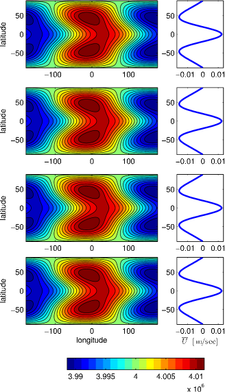
Figure 2.— Geopotential ($gh$) over the globe (left) and zonal-mean zonal wind (right) in four low-amplitude shallow-water models initialized with differing initial conditions corresponding to the four initial conditions in Figure 1: a rest state (top row), eastward equatorial jet (second row), westward equatorial jet (third row), and three-jet pattern (fourth row). Units of colorbar are $\rm m^{2}\,s^{-2}$. These are models SW1, SW2, SW3, and SW4 from top to bottom, respectively. These are snapshots, shown at 100 days, after the models have reached equilibrium. Despite the different initial conditions, the models all converge to the identical steady state.

Figure 3 illustrates an example of a high-amplitude model, where $\Delta h_{\rm eq}/H=0.5$, $\tau_{\rm rad}=0.1\rm\,day$, and $\tau_{\rm drag}\to\infty$ (meaning there is no explicit large-scale drag in the upper layer; as described in Showman & Polvani (2011), such a model still equilibrates because of interactions with the quiescent lower layer). Again, the four models in Figure 3 are integrated from the four initial conditions shown in Figure 1, corresponding to a rest state (top row), eastward equatorial jet (second row), westward equatorial jet (third row), and three-jet pattern (fourth row). All of the models equilibrate to the same final state, with significant day-night differences in geopotential and an overall pattern of eastward-equatorward phase tilts, particularly on the dayside, which is the result of the standing, planetary-scale Rossby and Kelvin waves. Because of the large forcing amplitude, short $\tau_{\rm rad}$, and absence of large-scale drag, the zonal-mean zonal wind equilibrates to fast speeds of $1\rm\,km\,s^{-1}$ in the core of the superrotating equatorial jet that emerges (Figure 3). Again, we emphasize that the speed and amplitude of this equilibrated jet is totally independent of whether the initial condition contained an eastward jet, a westward jet, multiple jets, or no jets at all.

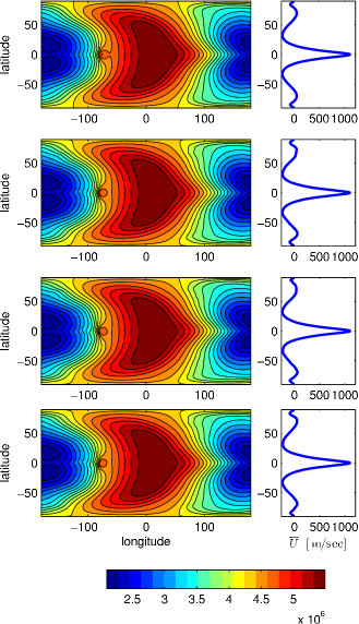
Figure 3.— Geopotential ($gh$) over the globe (left) and zonal-mean zonal wind (right) in four high-amplitude shallow-water models initialized with differing initial conditions corresponding to the four initial conditions in Figure 1: a rest state (top row), eastward equatorial jet (second row), westward equatorial jet (third row), and three-jet pattern (fourth row). Units of colorbar are $\rm m^{2}\,s^{-2}$. These are models SW5, SW6, SW7, and SW8 from top to bottom, respectively. These are snapshots, shown at 1000 days, after the models have reached equilibrium. Despite the different initial conditions, the models all converge to the same statistical steady state.

Figure 4 further quantifies the similarity between the final states of otherwise identical models initialized with differing initial conditions. The left panels show the differences in the geopotential, at a given time, in the equilibrated states of two models integrated with identical forcing parameters but differing initial conditions, i.e., $[gh_{\rm model\,a}(\lambda,\phi,t_{1})-gh_{\rm model\,b}(\lambda,\phi,t_{1})]/gh_{\rm model\,a}(\lambda,\phi,t_{1})$), where “model a” and “model b” are the two models being compared, and $t_{1}$ is some late time after the runs are equilibrated. The right panels overplot the zonal-mean zonal wind for these two models in red and green. The top row represents the differences between two low-amplitude models (SW2 and SW3) while the bottom row shows the differences between two high-amplitude cases (SW5 and SW8).

When the forcing amplitude is low and the solutions are steady, the final solutions are identical, in a point-to-point sense, to a precision of literally $\sim$$10^{-12}$–$10^{-13}$ (top row of Figure 4). Fractional differences are a few$\,\times 10^{-13}$ over most of the globe but rise to a few$\,\times 10^{-12}$ in a few localized regions (particularly near the poles). These miniscule differences are numerical, resulting from a combination of roundoff and discretization error, and indicate that, for all practical purposes, the solutions of these different models are truly identical despite the vastly different initial conditions. The equilibrated zonal-mean zonal wind profiles are likewise so similar that the red curve is precisely covered by the overlying green curve (top right panel of Figure 4).

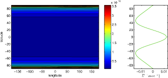
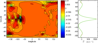
Figure 4.— Differences between the models in Figures 2 and 3. Left: Fractional differences in geopotential ($gh$) between two otherwise identical models initialized with different initial conditions. Top left plots $(gh_{\rm SW2}-gh_{\rm SW3})/gh_{\rm SW2}$, whereas bottom left plots $(gh_{\rm SW5}-gh_{\rm SW8})/gh_{\rm SW5}$, both at a specific instant in time (100 days in the top row, 1000 days in the bottom row). Here, $gh_{\rm X}$ refers to the geopotential of model X. Right: Zonal-mean zonal wind from the two models shown in the corresponding left panels. Top right shows SW2 (green curve) and SW3 (red curve) at 100 days while bottom right shows SW5 (green curve) and SW8 (red curve) at 1000 days. The figure demonstrates that low-amplitude cases (SW2 and SW3) converge to the identical steady state, with fractional differences of $\sim$$10^{-12}$ or less; high-amplitude cases, however, converge to states that, at any given instant, can differ at specific points by up to $\sim$2%, although the zonal-mean zonal winds are still nearly identical.

Although Figure 3 demonstrates that high-amplitude models likewise equilibrate to nearly identical states, tiny differences become apparent when one compares in more detail. The bottom row of Figure 4 quantifies these differences. In this case, the fractional point-to-point differences at a given time between otherwise identical models initialized with differing initial conditions (in this case SW5 and SW8) reaches $\sim$1% in specific regions, particularly on the nightside. One can ask whether this is a true difference in the statistical steady states between these models or whether it rather results from time variability that might induce a slight randomness around a single statistical steady state. To address this question, Figure 5 shows the differences between two different snapshots at different times within a given model integration. In the bottom row, these differences are likewise seen to reach $\sim$1%, with a spatial pattern extremely similar to that seen in the bottom row of Figure 4. This comparison indicates that the model-model differences shown in Figure 4 are the simple result of time variability and not the result of any fundamental sensitivity of the statistical steady state to initial condition. Indeed, the differences between the time-averages of the same two models are much smaller than the differences between their instantaneous snapshots displayed in Figure 4 (not shown), confirming that the statistical steady states are essentially identical for these models. We also note that, even at a given time, the two models have nearly identical zonal-mean zonal wind profiles (Figure 4, lower right panel), indicating that even the instantaneous point-to-point variability has little effect on the zonal-mean state.

We emphasize that the results shown are not specific to the particular parameters illustrated in the figures but rather are general. The wide variety of models we have performed all confirm the essential point made here, namely, the insensitivity of this forced shallow-water model to initial conditions.

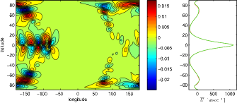
Figure 5.— Differences between a given high-amplitude shallow-water model, SW6, at two different points in time (900 and 1000 days), after the models have reached statistical steady state. Left panel shows the fractional geopotential differences, i.e., $(gh_{\rm 900days}-gh_{\rm 1000days})/gh_{\rm 900days}$, whereas right panel shows the zonal-mean zonal wind at 900 days (green curve) and 1000 days (red curve). These temporal differences within a given model are similar to the model-model differences shown in the bottom row of Figure 4, demonstrating that those differences result from time variability rather than sensitivity of the statistical steady state to initial conditions.

3. three-dimensional model

3.1. Model description

We now consider 3D models of the atmospheric circulation. As in most previous investigations, we adopt the primitive equations. We solve the equations using the MITgcm, which is a state-of-the-art circulation model (Adcroft et al., 2004) that Showman et al. (2009) adapted for application to hot Jupiters. The horizontal momentum, vertical momentum, continuity, and thermodynamic energy equations are, using pressure as a vertical coordinate,

$${d{\bf v}\over dt}=-\nabla\Phi-f{\bf k}\times{\bf v}+{\cal D}_{\bf v}$$ (6)

$${\partial\Phi\over\partial p}=-{1\over\rho}$$ (7)

$$\nabla\cdot{\bf v}+{\partial\omega\over\partial p}=0$$ (8)

$${dT\over dt}={q\over c_{p}}+{\omega\over\rho c_{p}}$$ (9)

where ${\bf v}$ is the horizontal velocity on constant-pressure surfaces, $\omega\equiv dp/dt$ is the vertical velocity in pressure coordinates, $\Phi$ is the gravitational potential on constant-pressure surfaces, $f\equiv 2\Omega\sin\phi$ is the Coriolis parameter, $\Omega$ is the planetary rotation rate, ${\bf k}$ is the local vertical unit vector, $q$ is the thermodynamic heating rate ($\rm\,W\rm\,kg^{-1}$), and $T$, $\rho$, $c_{p}$ are the temperature, density, and specific heat at constant pressure. $\nabla$ is the horizontal gradient evaluated on constant-pressure surfaces, and $d/dt=\partial/\partial t+{\bf v}\cdot\nabla+\omega\partial/\partial p$ is the material derivative (including curvature terms in spherical geometry). The term $\cal D_{\bf v}$ is a velocity damping term, including a Shapiro filter to maintain numerical stablity (which has only a small effect on the large-scale flow), and optionally, an explicit large-scale frictional drag term (see below). Eq (9) is actually solved in an alternate form,

$${d\theta\over dt}={\theta\over T}{q\over c_{p}}$$ (10)

where $\theta=T(p/p_{0})^{\kappa}$ is the potential temperature (a measure of entropy), $\kappa$ is the ratio of gas constant to specific heat at constant pressure, and $p_{0}$ is a reference pressure (note that the dynamics are independent of the choice of $p_{0}$). The dependent variables ${\bf v}$, $\omega$, $\Phi$, $\rho$, $\theta$, and $T$ are functions of longitude $\lambda$, latitude $\phi$, pressure $p$ and time $t$.

Figure 6.— Forcing profiles used in the Newtonian heating/cooling scheme. Top: Radiative-equilibrium temperature profiles. Dashed curves show the radiative equilibrium temperature profile for the nightside ($T_{\rm night,eq}$, left curve) and substellar point (right curve). The solid curve shows $T_{\rm Iro}(p)$. The dotted curve shows the substellar-nightside radiative-equilibrium temperature difference, $\Delta T_{\rm eq}(p)$, assuming the temperature difference at the top, $\Delta T_{\rm eq,top}$, is $1000\rm\,K$. Bottom: Radiative time constant, $\tau_{\rm rad}$, versus pressure.

Showman et al. (2009) coupled the MITgcm to the multi-stream radiative transfer model of Marley & McKay (1999), which allows for accurate calculation of heating rates when the atmospheric composition and opacities are specified. In the present context, however, our goal is to characterize the sensitivity to initial conditions in the clearest possible context, and so rather than using this coupled model, we specify the radiative heating/cooling using a Newtonian cooling scheme, which relaxes the temperature toward a specified radiative-equilibrium temperature over a specified time constant:

$$\frac{q}{c_{p}}=-\frac{T(\lambda,\phi,p,t)-T_{\rm eq}(\lambda,\phi,p)}{\tau_{\rm rad}(p)}.$$ (11)

The Newtonian cooling scheme has been widely used in exoplanet studies (Showman & Guillot, 2002; Cooper & Showman, 2005; Showman et al., 2008; Menou & Rauscher, 2009; Rauscher & Menou, 2010; Perna et al., 2010; Thrastarson & Cho, 2010; Heng et al., 2011b).

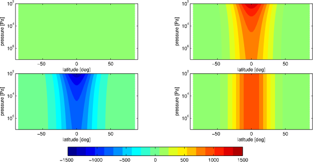
Figure 7.— Initial jet profiles adopted in our 3D models. Plotted is zonal-mean zonal wind of the initial condition, in $\rm m\,s^{-1}$, versus latitude and pressure. Initial conditions correspond to a rest state (upper left), eastward decaying jet (upper right), westward decaying jet (lower left), and eastward barotropic jet (lower right). We also tried westward barotropic jets in some models (not shown).

The radiative-equilibrium temperature, $T_{\rm eq}(\lambda,\phi,p)$, is defined as

$$T_{\rm eq}(\lambda,\phi,p)=\begin{cases}T_{\rm night,eq}(p)+\Delta T_{\rm eq}(p)\cos\lambda\cos\phi,&{\rm dayside};\\ T_{\rm night,eq}(p),&{\rm nightside}\end{cases}$$ (12)

where $T_{\rm night,eq}(p)+\Delta T_{\rm eq}$ is the radiative-equilibrium temperature at the substellar point and $\Delta T_{\rm eq}(p)$ is the difference in radiative-equilibrium temperature between the substellar point and the nightside. As written this expression takes the substellar point to be at longitude and latitude of $0^{\circ},0^{\circ}$. To specify the nightside profile, we further define $T_{\rm night,eq}(p)=T_{\rm Iro}-{\Delta T_{\rm eq}\over 2}$, where $T_{\rm Iro}(p)$ is the one-dimensional radiative-equilibrium temperature profile from Iro et al. (2005). These definitions then imply that the substellar radiative-equilibrium temperature profile is $T_{\rm Iro}+{\Delta T_{\rm eq}\over 2}$. Since radiative heating is strong at the top and weak at the bottom, it is important that $\Delta T_{\rm eq}(p)$ decreases with increasing pressure. For computational simplicity we specify $\Delta T_{\rm eq}(p)$ as a piecewise-continuous analytical function that is a constant, $\Delta T_{\rm eq,top}$, at pressures less than $p_{\rm eq,top}$; is zero at pressures exceeding $p_{\rm eq,bot}$; and varies linearly with log-pressure in between. For the models described in this paper, we take $\Delta T_{\rm eq,top}=1000\rm\,K$, $p_{\rm eq,top}=10^{-3}\rm\,bar$, and $p_{\rm eq,bot}=10\rm\,bar$; note that our key result—namely, insensitivity to initial conditions—does not depend on these precise values. The nightside and substellar radiative equilibrium profiles, as well as $T_{\rm Iro}$ and $\Delta T_{\rm eq}(p)$, are shown in Figure 6.

Likewise, the radiative time constant is expected to be a strong function of pressure, being short at the top and long at the bottom (Iro et al., 2005; Showman et al., 2008). For computational simplicity, we here assume that $\tau_{\rm rad}$ is a function of pressure alone, and we again define a piecewise-continuous analytic function that allows such a downward-increasing behavior: we take $\tau_{\rm rad}(p)$ to be a constant, $\tau_{\rm rad,top}$, at $p\leq p_{\rm rad,top}$; another constant, $\tau_{\rm rad,bot}$, at $p\geq p_{\rm rad,bot}$; and we assume that $\log\tau_{\rm rad}$ varies linearly with $\log p$ in between. In this paper, we take $p_{\rm rad,top}=10^{-2}\rm\,bar$ and $p_{\rm rad,bot}=10\rm\,bar$. We explore several values for $\tau_{\rm rad,top}$ and $\tau_{\rm rad,bot}$ in different models, with $\tau_{\rm rad,top}$ generally chosen to be short and $\tau_{\rm rad,bot}$ chosen to be long. Again, our key results are not dependent on the precise values. The profile of $\tau_{\rm rad}$ for one such model is shown in Figure 6.

In our models, we also include a simple frictional drag scheme near the bottom of the domain. This might crudely represent the effects of “magnetic drag” associated with the partial ionization expected at temperatures exceeding $\sim$$1500\rm\,K$ (Perna et al., 2010; Menou, 2012), which occur in our model at pressures exceeding $\sim$$1\rm\,bar$ (see Figure 6). From a more practical perspective, such frictional drag also forces the flow to equilibrate in a reasonable integration time. When studying sensitivity to initial conditions, it is particularly important to ensure that the models have reached equilibrium, and this is aided by including such a drag scheme. The drag is introduced on the righthand side of Equation (6) and takes the form $-k_{v}{\bf v}$, where $k_{v}(p)$ is a pressure-dependent drag coefficient. The drag coefficient is zero at pressures less than $p_{\rm drag,top}$ and equal to $k_{F}(p-p_{\rm drag,top})/(p_{\rm bot}-p_{\rm drag,top})$ at $p\geq p_{\rm drag,top}$, where $p_{\rm drag,top}$ is the lowest pressure of the region experiencing drag, $p_{\rm bot}$ is the mean pressure at the bottom of the domain, and $k_{F}$ is a constant (this formulation of drag is extremely similar to that of Held & Suarez, 1994). This formulation implies that the drag coefficient increases linearly with pressure from zero at $p_{\rm drag,top}$ to $k_{F}$ at the bottom of the domain. Motivated by expectations that magnetic drag is most important only at temperatures exceeding $\sim$$1500\rm\,$K, we take $p_{\rm drag,top}=1\rm\,bar$ in most models, although we also explore values of $10\rm\,bar$ to determine the sensitivity to drag scheme. The qualitative structure of the equilibrated dynamical state is not strongly sensitive to $k_{F}$; here, we explore values of $0.1$ and $0.01\rm\,day^{-1}$, implying characteristic drag timescales of 10 and 100 days near the bottom.

Overall, our choices of $\Delta T_{\rm eq}(p)$, $\tau_{\rm rad}(p)$ and drag scheme described above are motivated by three overarching goals: (1) to ensure that the radiative heating/cooling rates (expressed in $\rm K\,s^{-1}$) are large at the top but decrease rapidly with increasing pressure to very small values at the bottom, as expected on real hot Jupiters; (2) to produce equilibrated circulation patterns qualitatively resembling those from models that couple the dynamics to radiative transfer (i.e., Showman et al., 2009; Heng et al., 2011a; Rauscher & Menou, 2012; Perna et al., 2012), and (3) to ensure that the models equilibrate in finite time, as necessary to test sensitivity to initial conditions and to survey the parameter space. The first and second criteria generally lead to choices of $\tau_{\rm rad,top}=10^{4}$ or $10^{5}\rm\,s$ and $\tau_{\rm rad,bot}\gtrsim 10^{6}\rm\,s$, while the third criterion suggests $\tau_{\rm rad,bot}\lesssim 10^{8}\rm\,s$ and $p_{\rm drag,top}\lesssim 10\rm\,$bars. We note that our fomulation differs significantly from that of Thrastarson & Cho (2010), who choose $\Delta T_{\rm eq}$ and $\tau_{\rm rad}$ to be independent of pressure; although this assumption has the advantage of simplicity, it fails to satisfy criteria (1) and (2).

Table 2The properties of some 3D runs

Name	Initial condition	$\tau_{\rm rad,top}\rm\,(s)$	$\tau_{\rm rad,bot}\rm\,(s)$	$kF\rm\,(day^{-1})$	$p_{\rm drag,top}\rm\,(bar)$)
GCM1	Rest state	$10^{4}$	$10^{6}$	$0.1$	1
GCM2	Eastward decaying jet	$10^{4}$	$10^{6}$	$0.1$	1
GCM3	Westward decaying jet	$10^{4}$	$10^{6}$	$0.1$	1
GCM4	Eastward barotropic jet	$10^{4}$	$10^{6}$	$0.1$	1
GCM5	Rest state	$10^{5}$	$10^{6}$	$0.1$	1
GCM6	Eastward decaying jet	$10^{5}$	$10^{6}$	$0.1$	1
GCM7	Westward decaying jet	$10^{5}$	$10^{6}$	$0.1$	1
GCM8	Eastward barotropic jet	$10^{5}$	$10^{6}$	$0.1$	1

Following Thrastarson & Cho (2010), as well as our shallow-water models from Section 2, we initialize most of our 3D models with a zonally symmetric zonal flow whose latitude dependence is given by Equation (5) with $\sigma=\pi/9$ and $U=0$ (corresponding to a rest state), $1\rm\,km\,s^{-1}$ (corresponding to an eastward equatorial jet), or $-1\rm\,km\,s^{-1}$ (corresponding to a westward equatorial jet). In some cases, we assume this initial jet to be independent of pressure, while in others, we allow the jet to decay with pressure by multiplying the right side of Equation (5) by the function $1.6+\arctan[-(\log p-\log p_{\rm top})/\log p_{\rm top}]/1.6$, which causes the jets to decay from a peak speed of $\sim$$1.6\rm\,km\,s^{-1}$ at the top to $\sim$$400\rm\,m\,s^{-1}$ at the bottom of the domain. Figure 7 shows several of these initial conditions, laid out in a format that we will repeat, for easy comparison, when presenting results.

We adopt planetary parameters appropriate to hot Jupiters, including specific heat $\rm c_{p}=1.3\times 10^{4}\rm\,J\rm\,kg^{-1}\,{\rm K}^{-1}$, specific gas constant $3700\rm\,J\,kg^{-1}\,K^{-1}$, and a rotation period, gravity, and planetary radius of $3.024\times 10^{5}\,{\rm s}$, $9.36\rm\,m\,{\rm s}^{-2}$, and $9.437\times 10^{7}\,$m, respectively. These values are appropriate to HD 209458b, although we emphasize that our results are not sensitive to the precise values, and similar behavior would occur had choices appropriate to other typical hot Jupiters been made instead.

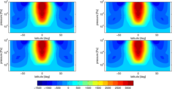
Figure 8.— Equilibrated zonal-mean zonal wind ($\rm m\,s^{-1}$) in four otherwise identical models with differing initial conditions. These four models adopt the initial conditions corresponding to the equivalent panels of Figure 7. Upper left, upper right, lower left, and lower right panels show models GCM1, GCM2, GCM3, and GCM4, initialized from a rest state, an eastward decaying jet, a westward decaying jet, and an eastward barotropic jet, respectively. The zonal averages shown here are time averaged from 694 to 1042 days. All four models adopt $\tau_{\rm rad,top}=10^{4}\rm\,s$, $\tau_{\rm rad,bot}=10^{6}\rm\,s$, $k_{F}=0.1\rm\,day^{-1}$, $p_{\rm drag,top}=1\rm\,bar$, and $\Delta T_{\rm eq,top}=1000\rm\,K$.

The MITgcm solves the equations using a finite-volume discretization on staggered Arakawa C grid (Arakawa & Lamb, 1977). Rather than the standard longitude/latitude coordinate system, we solve the equations using the cubed-sphere grid following Showman et al. (2009). The horizontal resolutions is C32 in most models, implying that each of the six “cube faces” has a resolution of $32\times 32$ finite-volume elements, which is roughly equal to a global resolution of $128\times 64$ in longitude and latitude. However, to ensure that our results are numerically converged and do not depend on these numerical details, we also performed some models at a resolution of C64 (i.e., $64\times 64$ cells on each cube face, corresponding to a global resolution of approximately $256\times 128$) and a resolution of C128 (i.e., $128\times 128$ on each cube face, corresponding to a global resolution of approximately $512\times 256$). The upper boundary is zero pressure and the bottom boundary is an impermeable surface. We adopt $N_{L}=40$ levels in the vertical; the bottom $N_{L}-1$ levels are evenly spaced in log-pressure between 200 bars at the bottom and 0.2 mbar at the top; the top layer extends from a pressure of 0.2 mbar to zero.

3.2. Results

As before, we explored a variety of models, with differing values of $\tau_{\rm rad,top}$, $\tau_{\rm rad,bot}$, $kF$, $p_{\rm drag,top}$ and initial condition. A small subset of these models, which are illustrated in subsequent figures, are shown in Table 2.

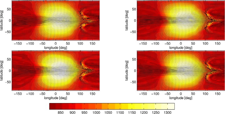
Figure 9.— Temperature (color scale, in K) and winds (arrows) for the same four models shown in Figure 8. This is at 30 mbar, which is near the infrared photosphere on a typical hot Jupiter. Panels show models GCM1 (upper left), GCM2 (upper right), GCM3 (lower left), and GCM4 (lower right), initialized with a rest state, eastward decaying jet, westward decaying jet, and eastward barotropic jet, respectively. These are snapshots at 1042 days. The final states are extremely similar.

In agreement with our shallow-water results, we find that the final, equilibrated state of our 3D models are independent of the initial condition. This is illustrated for a particular choice of forcing parameters (corresponding to models GCM1 to GCM4) in Figures 8 and 9. For easy comparison, the four panels in each of these figures adopt the initial conditions of the corresponding panels of Figure 7—a rest state (top left panel), eastward decaying jet (top right), westward decaying jet (bottom left), and eastward barotropic jet (bottom right). Figure 8 shows the zonal-mean zonal wind, while Figure 9 shows the temperature and two-dimensional velocity pattern at a pressure of $30\rm\,mbar$, for these four models after equilibrium has been reached. As can be seen, all four models exhibit extremely similar patterns of zonal wind, temperature pattern, and two-dimensional velocity structure despite the differing initial conditions. The momentum fluxes caused by the day-night thermal forcing drive a broad equatorial jet whose peak speeds exceed $3\rm\,km\,s^{-1}$ (Figure 8). The day-night temperature differences exceed $\sim$$800\rm\,K$ at the top of the model and are $500\rm\,K$ at 30 mbar (Figure 9). At low pressure, the short radiative time constant—$10^{4}\rm\,s$ in these models—leads to little longitudinal offset of the dayside hot region, although by 30 mbar the hot spot is displaced to the east of the substellar point by $\sim$$20^{\circ}$ longitude. Figure 10 shows the total kinetic energy over time, integrated over the entire domain, for these four models; the initial kinetic energies differ because of the differing initial jet profiles, but the models all converge to the same kinetic energy over time. Clearly, the models have lost memory of the initial condition and have all converged to the identical statistical steady state.

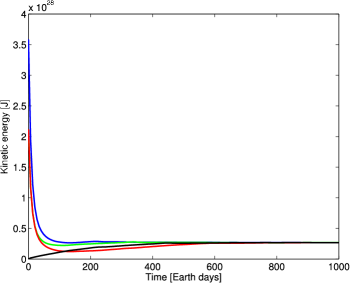
Figure 10.— Total kinetic energy, integrated over the model domain, for the four models GCM1 (black), GCM2 (green), GCM3 (red) and GCM4 (blue) which are initialized with different initial conditions but are otherwise the same. The initial kinetic energies differ greatly due to the differing initial conditions, but the model all converge to the same final state, independent of initial condition.

The lack of sensitivity to initial conditions is demonstrated with another example in Figures 11 and 12, which show models with a longer radiative time constant of $10^{5}\rm\,s$ in the upper part of the domain. As before, the figures depict the zonal-mean zonal wind (Figure 11) and the temperature and velocity patterns at 30 mbar (Figure 12) for four models—GCM5, GCM6, GCM7, and GCM8—initialized with the jet profiles shown in Figure 7. Except for the initial conditions, everything about the models are identical. Despite the vastly differing initial conditions, the models again all converge to the same final state. The equilibrated state exhibits a fast ($3\rm\,km\,s^{-1}$) equatorial jet, with day-night temperature differences that are hundreds of K at low pressure. Interestingly, because of the longer radiative time constant at the top, the day-night temperature difference in GCM5–GCM8 is smaller than in models GCM1–GCM4, and there is a larger eastward displacement of the dayside hot region relative to the substellar point. Thus, while it is clear that the response of our hot-Jupiter models do depend on forcing parameters, they do not depend on initial conditions.

Figure 11.— Zonal-mean zonal wind ($\rm m\,s^{-1}$) in four otherwise identical models with differing initial conditions. These four models adopt the initial conditions shown in Figure 7. Upper left, upper right, lower left, and lower right panels show models GCM5, GCM6, GCM7, and GCM8, initialized from a rest state, an eastward decaying jet, a westward decaying jet, and an eastward barotropic jet, respectively. Unlike Figure 8, this figure shows snapshots at 1042 days, giving a sense of the instantaneous variability in the zonal-mean zonal wind. In a time average, this variability averages out and the different models would look even more similar.

If one compares the panels in Figures 11 and 12 carefully, very slight differences become apparent; the peak speed at the core of the equatorial jet, for example, are not quite identical between the four panels. Likewise there are slight, second-order fluctuations in the pattern of the velocity vectors in Figure 9, particularly on the nightside within $\sim$$40^{\circ}$ latitude of the equator. These differences are the result of time-variability, which induces a slight randomness about the statistical steady state, rather than any fundamental sensitivity to initial conditions. This is demonstrated in Figure 13, where the zonal-mean zonal wind from model GCM8 is shown at four different times after the model has reached statistical steady state. The figure shows that the equatorial jet fluctuates slightly in time; the amplitude of these fluctuations is comparable to the inter-model differences seen in Figure 11. A temporal average of the temperature or velocity patterns removes these random fluctuations and yields a pattern that is essentially identical between models with the same forcing parameters but differing initial conditions.

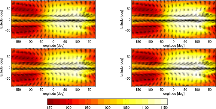
Figure 12.— Temperature at 30 mbar (color scale, in K) and winds (arrows) for the same four models shown in Figure 11. Panels show models GCM5 (top left), GCM6 (top right), GCM7 (bottom left), and GCM8 (bottom right), initialized with a rest state, eastward decaying jet, westward decaying jet, and eastward barotropic jet, respectively. These are snapshots at 1042 days, and the slight differences between panels gives a sense of the time variability. In a time average, the different models look even more similar.

We also performed models with weaker damping and drag in the deep atmosphere, for example models with $\tau_{\rm rad,bot}$ of $10^{7}\rm\,s$, $kF$ of $0.01\rm\,day^{-1}$, and/or $p_{\rm drag,top}$ of $10\rm\,bar$ (not shown). We also performed some models with weaker day-night forcing, e.g., $\Delta T_{\rm eq}=100\rm\,K$ rather than 1000 K as for most of the models in this paper. Likewise, we also tried some qualitatively different initial conditions, such as models containing nonzero zonal flow over only a specified subset of longitudes. In each case, for a given set of forcing/damping parameters, the models equilibrate to a statistical steady state with no sensitivity to initial conditions.

The lack of sensitivity to initial conditions in our models is not an artifact of our model resolution or numerical damping (i.e., the Shapiro filter) but rather is a fundamental property of the system behavior over the range explored. We also integrated models with resolutions of C64 and C128, approximately equivalent to global resolutions of $256\times 128$ and $512\times 256$, respectively, in longitude and latitude. To the best of our knowledge, our C128 models, in particular, are higher resolution than any published three-dimensional models of hot Jupiters that include day-night thermal forcing to date. Initial conditions corresponding to rest states, eastward barotropic jets, and westward barotropic jets (identical to that shown in the lower right panel of Figure 7 but multiplied by $-1$) were explored. Figure 14 shows these results for the C128 models initialized with an eastward jet (left column) and a westward jet (right column). All of these models converged to a statistical steady state that is essentially identical, showing that memory of the initial condition has been lost. Instantaneous snapshots of the temperature field are extremely similar in overall structure (Figure 14, top row). The flow does exhibit some small-scale structure that is time-variable and differs from one snapshot to another (either between different simulations or at different times of a given simulation). Averaging in time to determine the statistical steady state leads to temperature and wind fields that are essentially identical regardless of the initial condition (Figure 14, middle and bottom rows). For a given set of forcing parameters, the overall pattern of temperature and winds are also extremely similar between our C32, C64, and C128 models, suggesting that numerical convergence has nearly been reached even by C32 (compare Figure 14 with Figures 11 and 12).

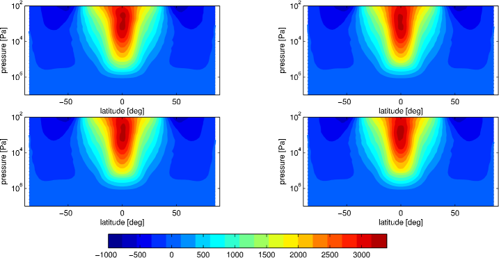
Figure 13.— Zonal-mean zonal wind ($\rm m\,s^{-1}$) at four different times for a single model, GCM8. Panels give snapshots at 833 days (top left), 903 days (top right), 972 days (bottom left), and 1042 days (bottom right). The differences result from time variability. These differences are at least as large as the model-to-model differences shown in Figure 11, indicating that those differences result from time variability rather than sensitivity of the statistical steady state to initial conditions.

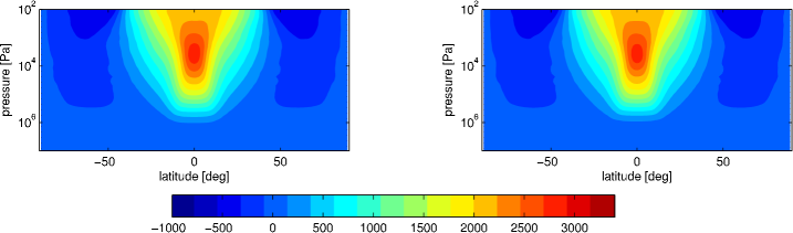
Figure 14.— Wind and temperature for two otherwise identical high-resolution models initialized with differing initial conditions. Resolution is C128, corresponding to a global grid of $512\times 256$ in longitude and latitude, with 40 vertical levels. Left column shows a model initialized with an initial eastward jet (like that in the lower right panel of Figure 7) while right column shows a model initialized with an initial westward jet (like that in the lower right panel of Figure 7 times $-1$). Physical parameters in both models are identical to those in low-resolution models GCM5–8 (i.e., $\tau_{\rm rad,top}=10^{5}\rm\,s$, $\tau_{\rm rad,bot}=10^{6}\rm\,s$, $kF=0.1\rm\,day^{-1}$, and $p_{\rm drag,top}=1\rm\,bar$). Top row: Snapshots of temperature (colorscale, K) and winds (arrows) on the 30-mbar level at a time of 1042 days. Middle row: Time average from 868 to 1042 days of temperature and winds at 30 mbars. Bottom row: Time average from 868 to 1042 days of zonal-mean zonal wind ($\rm m\,s^{-1}$). Models converge to the same statistical steady state regardless of initial condition. The statistical steady state is also extremely similar to those obtained in low-resolution C32 models with the same parameters (compare to Figures 11 and 12).

It is interesting to consider the situation where frictional drag is excluded (i.e., $kF=0$). Because no mass can enter or leave the model domain, and the top and bottom boundaries are free-slip in horizontal momentum, the absence of frictional drag implies the absence of any external torques acting on the system. In such a situation, the globally integrated angular momentum over the domain is conserved to within numerical accuracy. Therefore, a drag-free model initialized with an eastward jet will exhibit a different total angular momentum—for all time—than a drag-free model initialized from rest or from a westward jet. As a result, drag-free models initialized with differing angular momentum cannot converge to the same final state, because there is no mechanism to force their differing angular momenta to converge to a single value. However, it is important to emphasize that this situation is artificial: on a real planet the atmosphere will interact with the interior, leading to a torque on the atmosphere that allows the atmospheric state to adjust its angular momentum relative to the interior, and this will remove this initial-condition sensitivity on the atmospheric flow. In our shallow-water models (Section 2), the active layer interacts with an underlying (assumed quiescent) interior, and this explains why these models exhibit no sensitivity to initial condition even in the case where drag is excluded from the active layer (i.e., $\tau_{\rm drag}\to\infty$). In our 3D models, the application of frictional drag (i.e., non-zero $kF$) near the bottom is crudely intended to represent such an atmosphere-interior interaction and again explains the lack of sensitivity to initial conditions in those models. Even in the absence of drag, the existence of a deep, quiescent, inert layer at the bottom of the domain, as exists in many published hot-Jupiter models in the literature, can serve as a reservoir of mass and momentum that plays a similar role.

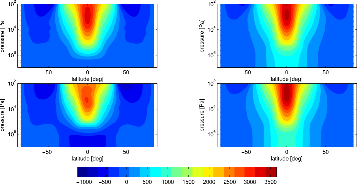
Figure 15.— Zonal-mean zonal wind ($\rm\,m\,s^{-1}$) in four models with no large-scale drag (i.e., $kF=0$) initialized from the four different initial conditions given in the corresponding panels of Figure 7 (rest state in upper left, decaying eastward jet in upper right, decaying westward jet in lower left, and barotropic eastward jet in lower right). All other physical and numerical parameters are identical to those of GCM5–GCM8. Because of the absence of drag, the angular momenta of the four runs are each constant in time (to within numerical errors) but are different from each other, and therefore the models do not converge to the same steady state. In particular, memory of the initial jet is retained at pressures exceeding 10 bars. The zonal averages shown here are time averaged from 694 to 1042 days.

Figures 15 and 16 illustrate the behavior when large-scale frictional drag is excluded. These models are identical to GCM5–GCM8 in all respects except that the drag coefficient $kF$ is set to zero (the models still include the Shapiro filter for numerical stability). As expected from the arguments above, the absence of drag means there is no mechanism for the angular momenta of the four models—which are initially different—to converge to the same value. Consistent with this expectation, Figure 15 shows that these models retain memory of the initial jet at pressures exceeding 10 bars. Interestingly, however, the jet profiles at pressures less than 1 bar are quite similar despite the differing initial conditions. In the observable atmosphere, the temperature patterns are likewise very similar for the different models; this is illustrated in Figure 16 at the 30-mbar level, which is near the infrared photosphere for a typical hot Jupiter. Because light curve and spectral observations are determined by the temperature structure at pressures less than 1 bar, this suggests that, in practice, observational predictions are not strongly sensitive to initial conditions even in this drag-free case, at least for the range of initial conditions considered here. We reiterate, however, that atmosphere-interior interaction on a real hot Jupiter would be expected to eliminate this sensitivity, as shown in our shallow-water models and in our 3D models with non-zero $kF$.

We also explored models where the radiative equilibrium temperature and radiative time constant are independent of depth, as in Thrastarson & Cho (2010). These models exhibit significant large-amplitude time variability that is qualitatively different from the other models presented in this paper. When large-scale drag is included at the bottom of the domain (i.e., non-zero $kF$), time averages of these solutions show that the statistical steady states are essentially identical regardless of the initial condition employed—despite the strong time variability. When drag is excluded, we find, as described above, that models whose initial conditions exhibit different angular momentum are unable to converge to the same time-mean state. Regardless, interaction between the flow and the bottom boundary seems to play a crucial role in the dynamics when $T_{\rm eq}$ and $\tau_{\rm rad}$ are independent of pressure—an aspect which is unrealistic for hot Jupiters, whose atmospheres are not underlain by impermeable surfaces. When the radiative equilibrium temperature profiles and radiative time constant are independent of pressure, the flow exhibits strong horizontal variations in entropy on the lower boundary. As is well known, the existence of horizontal entropy variations against an impermeable surface tend to make a flow much more baroclinically unstable (see, e.g., Vallis, 2006, Chapter 6). Such instabilities can lead to significant time variability, particularly when the Rossby deformation radius is global in scale, and this may help to explain the large degree of temporal variability in these models as well as the models of Thrastarson & Cho (2010). By comparison, our nominal models (e.g., GCM1 through GCM8) are set up so that the thermal forcing and horizontal entropy gradients are weak at the lower boundary; this helps to avoid such lower-boundary instabilities, which are artificial in the context of a gas giant.

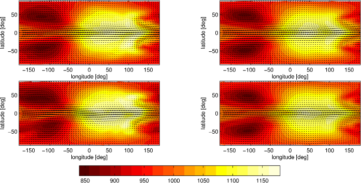
Figure 16.— Temperature at 30 mbar (color scale, in K) and winds (arrows) for the same four drag-free models shown in Figure 15. (The initial conditions of the four models correspond to a rest state in upper left, decaying eastward jet in upper right, decaying westward jet in lower left, and barotropic eastward jet in lower right.) These are snapshots at 1042 days. Interestingly, despite the differences in zonal-jet structure at pressures exceeding 10 bars in the four models, the temperature structure at 30 mbar—near the infared photosphere on a typical hot Jupiter—are quite similar.

4. Discussion and Conclusions

We explored the sensitivity to initial conditions of three-dimensional models of synchronously rotating hot Jupiters with day-night thermal forcing. The thermal forcing was chosen to be strong at the top and weak at the bottom, as must occur on real hot Jupiters. Models were integrated from rest and from various eastward and westward jet profiles with speeds up to $\sim$$1.5\rm\,km\,s^{-1}$. In all models explored, we found that the statistical steady states are independent of initial conditions—as long as the flow is anchored by interaction with a planetary interior so that the angular momentum of the atmosphere can adjust relative to that of the interior. In the context of atmosphere models, such interaction could be parameterized by frictional drag near the bottom of the domain or by allowing the atmosphere to exchange mass, energy, and angular momentum with a specified abyssal layer underlying the atmosphere. When such an interaction is included, all our models—for a given set of forcing parameters—converged to the same statistical steady state regardless of the initial condition employed. When the thermal forcing is strong, the circulation in the equilibrated state exhibits modest time variability that induces small-amplitude random fluctuations in any given realization. The statistical steady state itself, including not only the time-mean wind and temperature but the overall amplitude of these fluctuations, are independent of initial conditions when drag—or direct interaction with a specified abyssal layer—are included.

As described in the Section 1, the issue of initial-condition sensitivity is perhaps best thought of in terms of whether the atmospheric circulation exhibits a single, rather than multiple, stable equilibria. Taken at face value, our models suggest empirically that, for any given set of forcing and damping parameters, there exists only one stable equilibrium—at least for the range of forcing, damping, and planetary parameters explored here. We have intentionally chosen forcing and planetary parameters similar to those appropriate to typical hot Jupiters, including HD 189733b and HD 209458b, as explored by a number of authors (Showman et al., 2009; Heng et al., 2011b, a; Perna et al., 2012; Rauscher & Menou, 2012). Therefore, we expect our fundamental result—the lack of sensitivity to initial conditions—to apply generally to the regimes explored in those papers.

In this context, it is interesting that our findings differ so drastically from those of Thrastarson & Cho (2010). Their models differ from ours in two important ways: they lack large-scale drag, and the profiles of $T_{\rm eq}$ and $\tau_{\rm rad}$ in their Newtonian-cooling scheme are independent of pressure. Both these differences seem to contribute to the differences in their results relative to those presented here. In particular, the absence of frictional drag in a 3D model with free-slip boundary conditions and no mass fluxes through the boundaries implies the absence of any external torques that could change the globally integrated angular momentum over time. Thus, the globally integrated angular momentum of such a model will be conserved over time to within numerical accuracy. Since initial conditions corresponding to eastward jets, westward jets, and rest states exhibit different angular momenta, there is thus no mechanism to force those models to converge to the same angular momentum and hence final state. In practice, we found that this sensitivity is not strong in the observable atmosphere for the range of initial conditions explored here. Nevertheless, it may be stronger when $T_{\rm eq}$ and $\tau_{\rm rad}$ are constant with depth, as is the case in most of Thrastarson & Cho (2010)’s models.

Regardless, our results highlight the importance of anchoring the flow to an assumed planetary interior, either via the application of frictional drag; the introduction of a deep, quiescent layer at the bottom of the domain (as exists in many published 3D hot Jupiter models), or the explicit assumption of an abyssal layer underlying the active layer (as exists in 1-1/2 layer shallow-water models). Only in this way can the atmosphere experience net torques that allow it to adjust angular momentum over time, allowing models with differing initial angular momenta to converge to a single statistical steady state.

Overall, our results indicate that specification of initial conditions is not a source of uncertainty in atmospheric circulation models of hot Jupiters, at least over the parameter range explored here. This supports the continued use of hot-Jupiter GCMs for understanding dynamical mechanisms, explaining observations, and making predictions to help guide future observations. That said, our results, as well as those of numerous previous publications, show that details of the radiative forcing and frictional damping significantly affect the flow structure, including the qualitative dynamical regime, wind speeds, day-night temperature differences, and longitudinal offsets of any hot or cold regions. State-of-the-art GCMs now exist that include detailed non-grey radiative transfer (Showman et al., 2009) as well as simpler, faster, gray treatments (Heng et al., 2011a; Rauscher & Menou, 2012; Perna et al., 2012). By comparison, our understanding of how to specify frictional drag is less well developed, and areas such as inclusion of clouds, sub-gridscale parameterizations of turbulent mixing, and coupling to chemistry have received little attention. Continued model development in these areas, and comparison of such models to observations, should improve our ability to discern the physical and dynamical regimes of these fascinating worlds.

References

- Adcroft et al. (2004) Adcroft, A., Campin, J.-M., Hill, C., & Marshall, J. 2004, Monthly Weather Review, 132, 2845
- Arakawa & Lamb (1977) Arakawa, A., & Lamb, V. 1977, Methods in Computational Physics, 17, 173
- Budyko (1969) Budyko, M. I. 1969, Tellus, 21, 611
- Charbonneau et al. (2008) Charbonneau, D., Knutson, H. A., Barman, T., Allen, L. E., Mayor, M., Megeath, S. T., Queloz, D., & Udry, S. 2008, ApJ, 686, 1341
- Cho & Polvani (1996) Cho, J. Y.-K., & Polvani, L. M. 1996, Science, 8, 1
- Cooper & Showman (2005) Cooper, C. S., & Showman, A. P. 2005, ApJ, 629, L45
- Cooper & Showman (2006) —. 2006, ApJ, 649, 1048
- Cowan et al. (2007) Cowan, N. B., Agol, E., & Charbonneau, D. 2007, MNRAS, 379, 641
- Dobbs-Dixon et al. (2010) Dobbs-Dixon, I., Cumming, A., & Lin, D. N. C. 2010, ApJ, 710, 1395
- Dobbs-Dixon & Lin (2008) Dobbs-Dixon, I., & Lin, D. N. C. 2008, ApJ, 673, 513
- Dowling & Ingersoll (1989) Dowling, T. E., & Ingersoll, A. P. 1989, Journal of Atmospheric Sciences, 46, 3256
- Hack & Jakob (1992) Hack, J. J., & Jakob, R. 1992, Description of a global shallow water model based on the spectral transform method, Tech. rep., National Center for Atmospheric Research Technical note NCAR/TN-343+STR, Boulder, CO
- Harrington et al. (2006) Harrington, J., Hansen, B. M., Luszcz, S. H., Seager, S., Deming, D., Menou, K., Cho, J. Y.-K., & Richardson, L. J. 2006, Science, 314, 623
- Harrington et al. (2007) Harrington, J., Luszcz, S., Seager, S., Deming, D., & Richardson, L. J. 2007, Nature, 447, 691
- Held & Suarez (1994) Held, I. M., & Suarez, M. J. 1994, Bulletin of the American Meteorological Society, vol. 75, Issue 10, pp.1825-1830, 75, 1825
- Heng et al. (2011a) Heng, K., Frierson, D. M. W., & Phillipps, P. J. 2011a, MNRAS, 418, 2669
- Heng et al. (2011b) Heng, K., Menou, K., & Phillipps, P. J. 2011b, MNRAS, 413, 2380
- Iro et al. (2005) Iro, N., Bézard, B., & Guillot, T. 2005, A&A, 436, 719
- Knutson et al. (2008) Knutson, H. A., Charbonneau, D., Allen, L. E., Burrows, A., & Megeath, S. T. 2008, ApJ, 673, 526
- Knutson et al. (2007) Knutson, H. A., et al. 2007, Nature, 447, 183
- Lewis et al. (2010) Lewis, N. K., Showman, A. P., Fortney, J. J., Marley, M. S., Freedman, R. S., & Lodders, K. 2010, ApJ, 720, 344
- Li & Goodman (2010) Li, J., & Goodman, J. 2010, ArXiv e-prints
- Marley & McKay (1999) Marley, M. S., & McKay, C. P. 1999, Icarus, 138, 268
- Mayor & Queloz (1995) Mayor, M., & Queloz, D. 1995, Nature, 378, 355
- Menou (2012) Menou, K. 2012, ApJ, 745, 138
- Menou & Rauscher (2009) Menou, K., & Rauscher, E. 2009, ApJ, 700, 887
- Perna et al. (2012) Perna, R., Heng, K., & Pont, F. 2012, ApJ, 751, 59
- Perna et al. (2010) Perna, R., Menou, K., & Rauscher, E. 2010, ApJ, 719, 1421
- Pierrehumbert (2010) Pierrehumbert, R. T. 2010, Principles of Planetary Climate (Cambridge University Press)
- Polvani et al. (1995) Polvani, L. M., Waugh, D. W., & Plumb, R. A. 1995, Journal of Atmospheric Sciences, 52, 1288
- Rauscher & Menou (2010) Rauscher, E., & Menou, K. 2010, ApJ, 714, 1334
- Rauscher & Menou (2012) —. 2012, ApJ, 745, 78
- Scott & Polvani (2007) Scott, R. K., & Polvani, L. 2007, J. Atmos. Sci, 64, 3158
- Scott & Polvani (2008) Scott, R. K., & Polvani, L. M. 2008, Geophys. Res. Lett., 35, L24202
- Showman (2007) Showman, A. P. 2007, J. Atmos. Sci., 64, 3132
- Showman et al. (2008) Showman, A. P., Cooper, C. S., Fortney, J. J., & Marley, M. S. 2008, ApJ, 682, 559
- Showman et al. (2012) Showman, A. P., Fortney, J. J., & Lewis, N. 2012, ApJ, submitted to ApJ
- Showman et al. (2009) Showman, A. P., Fortney, J. J., Lian, Y., Marley, M. S., Freedman, R. S., Knutson, H. A., & Charbonneau, D. 2009, ApJ, 699, 564
- Showman & Guillot (2002) Showman, A. P., & Guillot, T. 2002, A&A, 385, 166
- Showman & Polvani (2010) Showman, A. P., & Polvani, L. M. 2010, Geophys. Res. Lett., 37, 18811
- Showman & Polvani (2011) —. 2011, ApJ, 738, 71
- Thrastarson & Cho (2010) Thrastarson, H. T., & Cho, J. 2010, ApJ, 716, 144
- Thrastarson & Cho (2011) Thrastarson, H. T., & Cho, J. Y. 2011, ApJ, 729, 117
- Vallis (2006) Vallis, G. K. 2006, Atmospheric and Oceanic Fluid Dynamics: Fundamentals and Large-Scale Circulation (Cambridge Univ. Press, Cambridge, UK)
- Watkins & Cho (2010) Watkins, C., & Cho, J. 2010, ApJ
- Wright et al. (2011) Wright, J. T., et al. 2011, PASP, 123, 412