Quintom phase-space: beyond the exponential potential

Abstract

We investigate the phase-space structure of the quintom dark energy paradigm in the framework of spatially flat and homogeneous universe. Considering arbitrary decoupled potentials, we find certain general conditions under which the phantom dominated solution is late time attractor, generalizing previous results found for the case of exponential potential. Center Manifold Theory is employed to obtain sufficient conditions for the instability of de Sitter solution either with phantom or quintessence potential dominance.

I Introduction

Recent cosmological observations point to an strong evidence for an spatially flat and accelerated expanding universe Riess2011 ; Komatsu2011 ; Reid2010 . Despite the great agreement of observations with the concordance model Li2011 , it is a fact that quintom model, whose Equation of State (EoS) can cross the cosmological constant barrier $w=-1$, is not exclude by observations Alam2004a ; Feng2005 ; Huterer2005 ; Nesseris2007 ; Jassal2010 ; Novosyadlyj2012 ; Novosyadlyj2012a ; Hinshaw2012 . A popular way to realize a viable quintom model and, at the same time, avoid the restrictions imposed by the No-Go Theorem Vikman2005 ; Hu2005 ; Caldwell2005 ; Xia2008 ; Cai2010 is the introduction of extra degrees of freedom. Following this recipe, the simple quintom paradigm requires a canonical quintessence scalar field $\sigma$ and simultaneously a phantom scalar field $\phi$ where the effective potential can be of arbitrary form, while the two components can be either coupled Zhang2006 or decoupled Feng2005 ; Guo2005 .

The properties of the quintom models have been studied from different points of view. Among them, the phase space studies, using the dynamical systems tools, are very useful in order to analyze the asymptotic behavior of the model. In quintom models this program have been carried out in Guo2005 ; Zhang2006 ; Lazkoz2006 ; Lazkoz2007 ; Setare2009 ; Setare2008a ; Setare2009c ; Cai2010 . In Guo2005 the decoupled case between the canonical and phantom field with an exponential potential is studied shown that the phantom-dominated scaling solution is the unique late-time attractor. In Zhang2006 the potential considers the interaction between the fields and shows that in the absence of interactions, the solution dominated by the phantom field should be the attractor of the system and the interaction does not affect its attractor behavior. This result is correct only in the case in which the existence of the phantom phase excludes the existence scaling attractors Lazkoz2006 . Some of these results were extended in Lazkoz2007 for arbitrary potentials. In Setare2009c the authors showed that all quintom models with nearly flat potentials converge to a single expression for EoS of dark energy, in addition, the necessary conditions for the determination of the direction of the $w=-1$ crossing was found.

The aim of this paper is to extend the study of Refs. Guo2005 ; Lazkoz2006 ; Lazkoz2007 ; Setare2009 ; Cai2010 -investigation of the dynamics of quintom cosmology- to include a wide variety of potential beyond the exponential potential without interaction between the fields, all of them can be constructed using the Bohm formalism Guzman2007 ; Socorro2010 ; Bohm1952 of the quantum mechanics under the integral systems premise, which is known as quantum potential approach. This approach makes it possible to identify trajectories associated with the wave function of the universe Guzman2007 when we choose the superpotential function as the momenta associated to the coordinate field $q$. This investigation was undertaken within the framework of the minisuperspace approximation to quantum theory when we investigate the dynamics of only a finite number of models. Here we make use of the dynamical systems tools to obtain useful information about the asymptotic properties of the model. In order to be able to analyze self-interaction potentials beyond the exponential one, we rely on the method introduced in Ref. Fang2009 in the context of quintessence models and that have been generalized to several cosmological contexts like: Randall-Sundrum II and DGP branes Leyva2009 ; Escobar2012a ; Escobar2012e , Scalar Field Dark Matter models Matos2009 , tachyon and phantom fields Quiros2010 ; Fang2010a ; Farajollahi2011 and loop quantum gravity Xiao2011j .

The plan of the paper is as follow: in section II we introduce the quintom model for arbitrary potentials and in section III we build the corresponding autonomous system. The results of the study of the corresponding critical points, their stability properties and the physical discussion are shown in section IV. The section V is devoted to conclusions. Finally, we include in the two appendices A and B the center manifold calculation of the solutions dominated by either the phantom or quintessence potential.

II The model

The starting action of our model, containing the canonical field $\sigma$ and the phantom field $\phi$, is Feng2005 ; Guo2005 ; Zhang2006 :

$$S=\int d^{4}x\sqrt{-g}\left(\frac{1}{2}R-\frac{1}{2}g^{\mu\nu}\partial_{\mu}\sigma\partial_{\nu}\sigma+V_{\sigma}(\sigma)+\right.$$

$$\left.+\frac{1}{2}g^{\mu\nu}\partial_{\mu}\phi\partial_{\nu}\phi+V_{\phi}(\phi)\right),$$ (1)

where we used natural units ($8\pi G=1$) and $V_{\sigma}(\sigma)$ and $V_{\phi}(\phi)$ are respectively the self interactions potential of the quintessence and phantom fields.

From this action the Friedmann equations for a flat geometry reads Guo2005 ; Zhang2006 :

$$H^{2}=\frac{1}{3}\left(\frac{\dot{\sigma}^{2}}{2}+V_{\sigma}(\sigma)-\frac{\dot{\phi}^{2}}{2}+V_{\phi}(\phi)\right)$$ (2)

$$\dot{H}=-\frac{1}{2}\left(\dot{\sigma}^{2}-\dot{\phi}^{2}\right)$$ (3)

where where $H=\frac{\dot{a}}{a}$ is the Hubble parameter and the dot denotes derivative with respect the time.

The evolution of the quintessence and phantom field are:

$$\ddot{\sigma}+3H\dot{\sigma}+V_{\sigma}^{\prime}(\sigma)=0$$ (4)

$$\ddot{\phi}+3H\dot{\phi}-V_{\phi}^{\prime}(\phi)=0,$$ (5)

where the coma denotes the derivative of a function with respect to their argument.

Additionally we can introduce the total energy density and pressure as:

$$\rho_{DE}=\rho_{\sigma}+\rho_{\phi},\;\;\;p_{DE}=p_{\sigma}+p_{\phi}$$ (6)

where

$$\rho_{\sigma}=\frac{\dot{\sigma}^{2}}{2}+V_{\sigma}(\sigma),\;\;\;\rho_{\phi}=-\frac{\dot{\phi}^{2}}{2}+V_{\phi}(\phi)$$ (7)

$$p_{\sigma}=\frac{\dot{\sigma}^{2}}{2}-V_{\sigma}(\sigma),\;\;\;p_{\phi}=-\frac{\dot{\phi}^{2}}{2}-V_{\phi}(\phi)$$ (8)

and its equation of state parameter is given by

$$w_{eff}=\frac{p_{\sigma}+p{\phi}}{\rho_{\sigma}+\rho_{\phi}}=\frac{\dot{\sigma}^{2}-\dot{\phi}^{2}-2V_{\sigma}(\sigma)-2V_{\phi}(\phi)}{\dot{\sigma}^{2}-\dot{\phi}^{2}+2V_{\sigma}(\sigma)+2V_{\phi}(\phi)}$$ (9)

and

$$\Omega_{\sigma}=\frac{\rho_{\sigma}}{\rho_{DE}},\;\;\Omega_{\phi}=\frac{\rho_{\phi}}{\rho_{DE}}$$ (10)

$$\Omega_{\sigma}+\Omega_{\phi}=1$$ (11)

are the the individual and total dimensionless densities parameters.

III The autonomous system

In order to study the dynamical properties of the system (2-5) we introduce the following dimensionless phase space variables to build an autonomous system Copeland1998 ; Chen2009 :

$$x_{\sigma}=\frac{\dot{\sigma}}{\sqrt{6}H},\\ x_{\phi}=\frac{\dot{\phi}}{\sqrt{6}H},\\ y_{\sigma}=\frac{\sqrt{V_{\sigma}(\sigma)}}{\sqrt{3}H},\\$$ (12)

$$\lambda_{\sigma}=-\frac{V_{\sigma}^{\prime}(\sigma)}{V_{\sigma}(\sigma)},\\ \lambda_{\phi}=-\frac{V_{\phi}^{\prime}(\phi)}{V_{\phi}(\phi)},\\$$ (13)

Notice that the phase space variables $\lambda_{\sigma}$ and $\lambda_{\phi}$ are sensitive of the kind of self interactions potential chosen for quintessence and phantom component, respectively and are introduced in order to be able to study arbitrary potentials. Applying the above dimensionless variables to the system (2-5) we obtain the following autonomous system:

$$\frac{dx_{\sigma}}{dN} = -3x_{\sigma}\left(1+x_{\phi}^{2}-x_{\sigma}^{2}\right)+\sqrt{\frac{3}{2}}y_{\sigma}^{2}\lambda_{\sigma}$$ (14)

$$\frac{dx_{\phi}}{dN} = -3x_{\phi}\left(1+x_{\phi}^{2}-x_{\sigma}^{2}\right)+$$ (15)

$$-\sqrt{\frac{3}{2}}\left(1+x_{\phi}^{2}-x_{\sigma}^{2}-y_{\sigma}^{2}\right)\lambda_{\phi}$$

$$\frac{dy_{\sigma}}{dN} = \frac{1}{2}y_{\sigma}\left(6x_{\sigma}^{2}-\sqrt{6}x_{\sigma}\lambda_{\sigma}-6x_{\phi}^{2}\right)$$ (16)

$$\frac{d\lambda_{\sigma}}{dN} = -\sqrt{6}x_{\sigma}f(\lambda_{\sigma})$$ (17)

$$\frac{d\lambda_{\phi}}{dN} = -\sqrt{6}x_{\phi}g(\lambda_{\phi})$$ (18)

where $N=\ln a$ is the number of e-foldings and $f(\lambda_{\sigma})=\lambda_{\sigma}^{2}(\Gamma_{\sigma}-1)$ and $g(\lambda_{\phi})=\lambda_{\phi}^{2}(\Gamma_{\phi}-1)$ where:

$$\Gamma_{\sigma}=\frac{V_{\sigma}(\sigma)V_{\sigma}^{\prime\prime}(\sigma)}{(V_{\sigma}^{\prime}(\sigma))^{2}},\;\;\;\Gamma_{\phi}=\frac{V_{\phi}(\phi)V_{\phi}^{\prime\prime}(\phi)}{(V_{\phi}^{\prime}(\phi))^{2}}$$ (19)

In order to get from the autonomous equation (14-18) a closed system of ordinary differential equation we have assumed that the funtions $\Gamma_{\sigma}$ and $\Gamma_{\phi}$ can be written as a function of the variables $\lambda_{\sigma}\in\mathbb{R}$ and $\lambda_{\phi}\in\mathbb{R}$ respectively Fang2009 .

The phase space for the autonomous dynamical system driven by de evolutions of Eqs. (14-18) can be defined as follows:

$$\Psi=\{(x_{\sigma},x_{\phi},y_{\sigma}):y_{\sigma}\geq 0,x_{\sigma}^{2}-x_{\phi}^{2}+y_{\sigma}^{2}\leq 1\}\times$$

$$\times\{(\lambda_{\sigma},\lambda_{\phi})\in\mathbb{R}^{2}\}$$ (20)

With the aim of explain the physical significance of the critical points of the autonomous system (14-18) we need to obtain the relevant cosmological parameters in terms of the dimensionless phase space variables (12). Following this, the cosmological parameter (9) and (10) can be expressed as

$$w_{eff}=-1+2x_{\sigma}^{2}-2x_{\phi}^{2}$$ (21)

$$\Omega_{\sigma}=x_{\sigma}^{2}+y_{\sigma}^{2},\;\;\ \Omega_{\phi}=1-x_{\sigma}^{2}-y_{\sigma}^{2},$$ (22)

while the deceleration parameter becomes

$$q=-\left[1+\frac{\dot{H}}{H^{2}}\right]=-1+3x_{\sigma}^{2}-3x_{\phi}^{2}.$$ (23)

IV Critical points and stability

The critical points of the system (14-15) are summarized in Table 1. The eigenvalues of the corresponding Jacobian matrices are show in Table 2. In both cases $\lambda_{\sigma}^{\ast}$ and $\lambda_{\phi}^{\ast}$ are the values which makes the functions $f(\lambda_{\sigma})=\lambda_{\sigma}^{2}\left(\Gamma_{\sigma}-1\right)$ and $g(\lambda_{\phi})=\lambda_{\phi}^{2}\left(\Gamma_{\phi}-1\right)$ vanish respectively.

Table 1: Properties of the critical points for the autonomous system (14-18)

$Label$	$x_{\sigma}$	$y_{\sigma}$	$x_{\phi}$	$\lambda_{\sigma}$	$\lambda_{\phi}$	Existence	$\Omega_{\sigma}$	$\Omega_{\phi}$	$q$	$w_{eff}$
$P_{1}^{\pm}$	$0$	$0$	$\pm i$	$\lambda_{\sigma}$	$\lambda_{\phi}^{\ast}$	Non real	$0$	$1$	$2$	$1$
$P_{2}^{\pm}$	$\pm 1$	$0$	$0$	$\lambda_{\sigma}^{\ast}$	$\lambda_{\phi}$	Always	$1$	$0$	$2$	$1$
$P_{3}^{\pm}$	$\pm\sqrt{1+x_{\phi}^{2}}$	$0$	$x_{\phi}$	$\lambda_{\sigma}^{\ast}$	$\lambda_{\phi}^{\ast}$	”	$1+x_{\phi}^{2}$	$-x_{\phi}^{2}$	$2$	$1$
$P_{4}$	$\frac{\lambda_{\sigma}^{\ast}}{\sqrt{6}}$	$\sqrt{1-\frac{(\lambda_{\sigma}^{\ast})^{2}}{6}}$	$0$	$\lambda_{\sigma}^{\ast}$	$\lambda_{\phi}$	$-\sqrt{6}\leq\lambda_{\sigma}^{\ast}\leq\sqrt{6}$	$1$	$0$	$-1+\frac{(\lambda_{\sigma}^{\ast})^{2}}{2}$	$-1+\frac{(\lambda_{\sigma}^{\ast})^{2}}{3}$
$P_{5}$	$0$	$0$	$0$	$\lambda_{\sigma}$	$0$	Always	$0$	$1$	$-1$	$-1$
$P_{6}$	$0$	$1$	$0$	$0$	$\lambda_{\phi}$	”	$1$	$0$	$-1$	$-1$
$P_{7}$	$0$	$y_{\sigma}$	$0$	$0$	$0$	$0<y_{\sigma}<1$	$y_{\sigma}^{2}$	$1-y_{\sigma}^{2}$	$-1$	$-1$
$P_{8}$	$0$	$0$	$-\frac{\lambda_{\phi}^{\ast}}{\sqrt{6}}$	$\lambda_{\sigma}$	$\lambda_{\phi}^{\ast}$	$\lambda_{\sigma}\in\mathbb{R}$	$0$	$1$	$-1-\frac{(\lambda_{\phi}^{\ast})^{2}}{2}$	$-1-\frac{(\lambda_{\phi}^{\ast})^{2}}{3}$

Table 2: Eigenvalues of the linear perturbation matrix associated to each of the critical points displayed in Table 1

$Label$	$m_{1}$	$m_{2}$	$m_{3}$	$m_{4}$	$m_{5}$
$P_{1}^{\pm}$	$3$	$0$	$0$	$\mp{i}\sqrt{6}g^{\prime}(\lambda_{\phi}^{\ast})$	$6\mp{i}\sqrt{6}\lambda_{\phi}^{\ast}$
$P_{2}^{\pm}$	$6$	$0$	$0$	$\mp\sqrt{6}f^{\prime}(\lambda_{\sigma}^{\ast})$	$3\mp\sqrt{\frac{3}{2}}\lambda_{\sigma}^{\ast}$
$P_{3}^{\pm}$	$0$	$-\sqrt{6}g^{\prime}(\lambda_{\phi}^{\ast}){x_{\phi}}$	$\mp\sqrt{6}{f^{\prime}(\lambda_{\sigma}^{\ast})}\sqrt{x_{\phi}^{2}+1}$	$3\mp\sqrt{\frac{3}{2}}\sqrt{x_{\phi}^{2}+1}\lambda_{\sigma}^{\ast}$	$6-\sqrt{6}x_{\phi}\lambda_{\phi}^{\ast}$
$P_{4}$	$0$	$-{f^{\prime}(\lambda_{\sigma}^{\ast})}\lambda\sigma^{\ast}$	$\left(\lambda\sigma^{\ast}\right)^{2}$	$\frac{1}{2}\left(\left(\lambda\sigma^{\ast}\right)^{2}-6\right)$	$\frac{1}{2}\left(\left(\lambda\sigma^{\ast}\right)^{2}-6\right)$
$P_{5}$	$-3$	$0$	$0$	$-\frac{3}{2}\left(1+\sqrt{1+\frac{4}{3}g(0)}\right)$	$-\frac{3}{2}\left(1-\sqrt{1+\frac{4}{3}g(0)}\right)$
$P_{6}$	$-3$	$0$	$0$	$-\frac{3}{2}\left(1+\sqrt{1-\frac{4}{3}f(0)}\right)$	$-\frac{3}{2}\left(1-\sqrt{1-\frac{4}{3}f(0)}\right)$
$P_{7}$	$0$	$\frac{1}{2}\left(-\sqrt{9-12f(0)y_{\sigma}^{2}}-3\right)$	$\frac{1}{2}\left(\sqrt{9-12f(0)y_{\sigma}^{2}}-3\right)$	$\frac{1}{2}\left(-\sqrt{9-12g(0)\left(y_{\sigma}^{2}-1\right)}-3\right)$	$\frac{1}{2}\left(\sqrt{9-12g(0)\left(y_{\sigma}^{2}-1\right)}-3\right)$
$P_{8}$	$0$	${g^{\prime}(\lambda_{\phi}^{\ast})}\lambda_{\phi}^{\ast}$	$-\frac{1}{2}\left(\lambda_{\phi}^{\ast}\right)^{2}$	$-\frac{1}{2}\left(\left(\lambda_{\phi}^{\ast}\right)^{2}+6\right)$	$-\frac{1}{2}\left(\left(\lambda_{\phi}^{\ast}\right)^{2}+6\right)$

As we see from Table 1, the points $P_{1}^{\pm}$ do not exist in the strict sense ($x_{\phi}$ is purely imaginary at the fixed points). Point $P_{5}$ is associated with a combination of a phantom potential whose first $\phi$-derivative vanishes at some/several point/points, i.e., $\lambda_{\phi}=0$ (this case include the exponential potential whose $\phi$-derivative at any order vanish everywhere) and an arbitrary self interaction potential for the quintessence component (arbitrary value of $\lambda_{\sigma}$). Point $P_{6}$ is associated with a combination of a quintessence potential whose first $\sigma$-derivative vanishes at some/several point/points, i.e., $\lambda_{\sigma}=0$ (this case include the exponential potential whose $\sigma$-derivative at any order vanish everywhere) and an arbitrary self interaction potential for the phantom component (arbitrary value of $\lambda_{\phi}$). Point $P_{7}$ is associated with a combination of a phantom potential whose first $\phi$-derivative vanishes at some/several point/points, i.e., $\lambda_{\phi}=0$ (this case include the exponential potential whose $\phi$-derivative at any order vanish everywhere) and a self interaction potential for the quintessence component whose first $\sigma$-derivative vanishes also at some/several point/points, i.e., $\lambda_{\phi}=0.$ It is worth noticing that the existence of points $P_{2}^{\pm}$, $P_{3}^{\pm}$, $P_{4}$, $P_{8}$ and $P_{9}$ depends of the concrete form of the potential. From the table of the eigenvalues, notice, besides, that all the points belongs to nonhyperbolic sets of critical point with a least one null eigenvalue.

IV.1 Stability of the critical points

Although all these critical points are shown in the Tables 1 here we have summarized their basic properties:

• $P_{1}^{\pm}$, $P_{2}^{\pm}$ and $P_{3}^{\pm}$ correspond to a solution dominated by the kinetic energy of the scalar fields (stiff fluid solution: $q=2$ and $\omega=1$). The exact dynamical behavior differs for each points. $P_{1}^{\pm}$ corresponds to a phantom kinetic energy dominated ($\Omega_{\sigma}=0$ and $\Omega_{\phi}=1$). However, these points have a purely imaginary value of $x_{\phi},$ thus, they do not exists in the strict sense. They have a three$-$dimensional center subspace and a two-dimensional unstable manifold ($m_{1}=3>0,\;\Re(m_{5})=6>0$). Thus they cannot be late-time attractors. $P_{3}^{\pm}$ represents an scaling regimen between the kinetics energies of the quintessence and phantom fields ($\Omega_{\sigma}=1+x_{\phi}^{2}$ and $\Omega_{\phi}=-x_{\phi}^{2}$). These points depend of the form of the potentials and under certain conditions they have a four dimensional unstable subspace which could correspond to the past attractor. However, this point is unphysical since $\Omega_{\phi}<0$ . $P_{2}^{\pm}$ is dominated by the quintessence kinetic term ($\Omega_{\sigma}=1$ and $\Omega_{\phi}=0$). Since they are non-hyperbolic due to the existence of two null eigenvalues, we are not able to extract information about their stability by using the standard tools of the linear dynamical analysis. However, since these points seems to be particular cases of $P_{3}^{\pm},$ they should share the same dynamical behavior. Because all of these points are nonhyperbolic, as we notice before, we cannot rely on the standard linear dynamical systems analysis for deducing their stability. Thus, we need to rely our analysis on numerical inspection of the phase portrait for specific potentials or use more sophisticated techniques like Center Manifold theory.

• $P_{4}$ is an scaling solution between the kinetic and the potential energy of the quintessence component of dark energy. This solution in sensitive to the explicit form of the potential. This is always a saddle equilibrium point in the phase space since $m_{2}=(\lambda_{\sigma}^{\ast})^{2}$ and $m_{4}=\frac{1}{2}((\lambda_{\sigma}^{\ast})^{2}-6)$ are of opposite sign in the existence region of this point. It represents an accelerated solution for a potential $V_{\sigma}(\sigma)$ whose function $f(\lambda_{\sigma})$ vanish for $\lambda_{\sigma}=\lambda_{\sigma}^{\ast}$ in the interval $-\sqrt{2}<\lambda_{\sigma}^{\ast}<\sqrt{2}$, leading to a $-1\leq w_{eff}<-1/3$. When $\lambda_{\sigma}^{\ast}=0$ the critical point $P_{4}$ becomes in $P_{6}$. In the regions $-\sqrt{6}\leq\lambda_{\sigma}^{\ast}\leq-\sqrt{2}$ or $\sqrt{2}\leq\lambda_{\sigma}^{\ast}\leq\sqrt{6}$, the critical point $P_{4}$ represents a non-accelerated phase. A very interesting issue of this critical point appears when, for an specific form of the quintessence potential, $\lambda_{\sigma}^{\ast}=\pm\sqrt{3}$, driving to $w_{eff}=0$. This means that the quintessence field is able to mimic the dark matter behavior.

• $P_{5}$, $P_{6}$ and $P_{7}$ represents solutions dominated by the potential energies of the potentials (all of them represent de Sitter solutions: $q=-1$ and $w_{eff}=-1$). Once again the exact dynamical nature differs from one point to the other: $P_{5}$ is dominated by the potential energy of the phantom component ($\Omega_{\sigma}=0$ and $\Omega_{\phi}=1$). Because of the existence of two null eigenvalues is not possible to conclude about its dynamics. However it has a three-dimensional stable manifold for $g(0)<0$ (in the interval $g(0)<-\frac{3}{4}$ it has to complex conjugated eigenvalues with negative real parts). In this cases it is worthy to analyze its stability using the center manifold theory. $P_{6}$ is a critical point dominated by the quintessence potential energy term ($\Omega_{\sigma}=1$ and $\Omega_{\phi}=0$), despite its nonhyperbolicity, it has three-dimensional stable manifold for $f(0)>0$ (in the case $f(0)>\frac{3}{4}$ it has to complex conjugated eigenvalues with negative real parts), thus, it is worthy to analyze its stability using the center manifold theory. $P_{7}$ denotes a segment (curve) of non-isolated fixed points, representing a scaling regimen between the quintessence and phantom potential ($\Omega_{\sigma}=y_{\sigma}^{2}$ and $\Omega_{\phi}=1-y_{\sigma}^{2}$). The existence of one non-zero eigenvalue is due to the fact that it is a curve of fixed points. As an invariant set of non-isolated singular points it is normally-hyperbolic, since the eigenvector associated to the zero eigenvalue, $(0,0,1,0,0)^{T},$ is tangent to the curve. Thus its stability is determined by the sign of the remaining non-null eigenvalues. Hence, it is stable for $0<y_{\sigma}<1,\;f(0)>0,\;g(0)<0$ or a saddle otherwise.

• $P_{8}$ is a line of fixed points parameterized by $\lambda_{\sigma}\in\mathbb{R}$. The existence of one non-zero eigenvalue is due to the fact that it is a curve of fixed points. As an invariant set of non-isolated singular points it is normally-hyperbolic, since the eigenvector associated to the zero eigenvalue, $(0,0,0,1,0)^{T},$ is tangent to the curve. Thus its stability is determined by the sign of the remaining non-null eigenvalues. From table 2 follows that $P_{8}$ admits a four dimensional stable subspace provided $g^{\prime}(\lambda_{\phi}^{\ast})\lambda_{\phi}^{\ast}<0$, thus, the invariant curve is stable. It represents accelerated solutions dominated by the phantom potential providing a crossing through the phantom divide ($\Omega_{\sigma}=0$ and $\Omega_{\phi}=1$). For every value of $\lambda_{\phi}^{\ast}$ this point provide the typical superaccelerated expansion of quintom paradigm ($w=-1-\frac{(\lambda_{\phi}^{\ast})^{2}}{3}$) the only exception occurs when $\lambda_{\phi}^{\ast}=0$ recovering the behavior of the de Sitter solution $P_{5}$ ($\omega=-1$). This line of critical point corresponds to the stable point $P$ in Guo2005 and B in Cai2010 (phantom dominated solution). Summarizing, the line $P_{8}$ is the late time stable attractor provided $g^{\prime}(\lambda_{\phi}^{\ast})\lambda_{\phi}^{\ast}<0$, otherwise, it is a saddle point.

IV.2 Cosmological consequences

As was shown in the previous subsection the autonomous systems only admits seven classes of critical points (some of them are actually curves) . The curves $P_{2}^{\pm}$ correspond to decelerated solutions, with $q=2$, where the Friedmann constraint (2) is dominated by the kinetic energy of the quintessence field with an equation of state of stiff type, $w_{eff}=1$. These solutions are only relevant a early times and should be unstable Copeland1998 . Unfortunately these critical points are nonhyperbolic (it has two zero eigenvalues) meaning that is not possible to obtain conclusions about its stability with the previous linear analysis. However the numerical analysis performed in the next subsection with a particular potentials confirm the previous results in literature.

An important result come from the stability of critical point $P_{4}$. This points exists if $-\sqrt{6}\leq\lambda_{\sigma}^{\ast}\leq\sqrt{6}$ and always behave as a saddle fixed point. The latter means that under certain initial conditions the orbits in the phase space will approach to this point spending some time in its vicinity before being repelled toward the attractor solution of the system. In the case of this point, as we mentioned before, if the quintessence potential fulfill the condition:

$$\lambda_{\sigma}^{\ast}=\pm\sqrt{3}$$ (24)

then the effective equation of state of this dark energy component would mimic pressureless fluid ($w_{eff}=0$), in other words: it will dynamically behave exactly as cold dark matter. The possibility of this dynamical characteristic impose a fine tunning over the shape of quintessence potentials and a priori there is no guarantee that all possible quintessence potentials may satisfy the above condition (24). Let’s note that in order to obtain the lower possible dimensionality of the phase space and to studying in a relatively simple way the effects of include arbitrary quintom potentials, we have neglected the contribution of the usual matter fields: radiation and baryonic matter in our model . As a result, a full study of important aspects, derived from realization of condition (24), such as: transition redshift between the decelerated and accelerated expansion phase and the clustering properties of this effective dark matter are beyond the present study and will be left for a future paper.

Another important characteristics of the model is the presence of three accelerated solutions, described by critical points $P_{5}$, $P_{6}$ and $P_{7}$. All of them are de Sitter solutions ($w_{eff}=-1$) dominated by the potentials of the scalar fields. As in the case of $P_{4}$, they behave as saddle points and, depending on the initial conditions, the orbits can evolve from the unstable fixed point ($P_{2}^{\pm}$ in our case) towards one or the other of the saddle points. A favorable scenario would be one in which the initial condition lead to an evolution from $P_{2}^{\pm}$ to the saddle point $P_{4}$ and then, the orbits tend to one of the de Sitter solutions $P_{5}$, $P_{6}$ or $P_{7}$ or to the late time phantom attractor ($P_{8}$). In terms of the cosmological evolution of the Universe, the above favorable scenario implies that the Universe started at early times from an stage dominated by the kinetic term of the quintessence, then evolve into an epoch dominated by the effective dark matter and finally enter in the final phase of accelerated expansion. This accelerated phase can be the de Sitter solutions or a phantom dominated solution ($w_{eff}<-1$) . This final stage of evolutions towards critical point $P_{8}$ is consistent with the recent joint results from WMAP+eCMB+BAO+$H_{0}$+SNe Hinshaw2012 which suggest a mild preference for a dark energy equation-of-state parameter in the phantom region ($w_{eff}<-1$).

Finally, in order to examine the stability of the nonhyperbolic points that cannot consistently be studied via the present linear analysis, we present a concrete example. We provide a numerical elaboration of the phase space orbits of the corresponding quintom model.

IV.3 $V(\sigma,\phi)=V_{0}\sinh^{2}(\alpha\sigma)+V_{1}\cosh^{2}(\beta\phi)$

This potential is derived, in a Friedmann-Robertson-Walker cosmological model, from canonical quantum cosmology under determined conditions in the evolution of our universe, using the bohmian formalism Guzman2007 . For this potential:

$$f(\lambda_{\sigma})=-\frac{\lambda_{\sigma}^{2}}{2}+2\alpha^{2},\;\;\lambda_{\sigma}^{\ast}=\pm 2\alpha,\;\;f^{\prime}(\lambda_{\sigma}^{\ast})=-{\lambda_{\sigma}^{\ast}}$$ (25)

and

$$g(\lambda_{\phi})=-\frac{\lambda_{\phi}^{2}}{2}+2\beta^{2},\;\;\lambda_{\phi}^{\ast}=\pm 2\beta,\;\;g^{\prime}(\lambda_{\phi}^{\ast})=-{\lambda_{\phi}^{\ast}}.$$ (26)

From the Table 2 and the equation (26) we see that the condition to ensure that Point $P_{8}$ has a four dimensional stable subspace is always satisfied due to the opposite signs between $\lambda_{\phi}^{\ast}$ and $g^{\prime}(\lambda_{\phi}^{\ast})$. In order to having achieved success scalar field dark matter domination era we need that $\lambda_{\sigma}^{\ast}=\pm\sqrt{3},$ since this is the only way to have a standard transient matter dominated solution ($P_{4}$). Recall that for the choice $\lambda_{\sigma}^{\ast}=\pm\sqrt{3},$ the standard quintessence dominated solution mimics dark matter ($w_{eff}=0$). Imposing the condition $\lambda_{\sigma}^{\ast}=\pm\sqrt{3},$ we have as a degree of freedom the potential parameter $\alpha$ that can be adjusted using (25). Furthermore, we impose one of the following conditions:

$$\lambda_{\sigma}^{\ast}=\sqrt{3},\;\lambda_{\phi}^{\ast}\leq-\sqrt{6},\;1<x_{\sigma}<\sqrt{1+\frac{6}{\left(\lambda_{\phi}^{\ast}\right)^{2}}}$$

or

$$\lambda_{\sigma}^{\ast}=\sqrt{3},\;-\sqrt{6}<\lambda_{\phi}^{\ast}<0,\;1<x_{\sigma}<\sqrt{2}$$

or

$$\lambda_{\sigma}^{\ast}=-\sqrt{3},\;\lambda_{\phi}^{\ast}\leq-\sqrt{6},\;-\sqrt{1+\frac{6}{\left(\lambda_{\phi}^{\ast}\right)^{2}}}<x_{\sigma}<-1$$

or

$$\lambda_{\sigma}^{\ast}=-\sqrt{3},\;-\sqrt{6}<\lambda_{\phi}^{\ast}<0,\;-\sqrt{2}<x_{\sigma}<-1.$$

to guarantee that the stiff matter type solution of the quintom cosmology be the past-attractor.

To finish this section let’s discuss some numerical elaborations. In the figure 1 are presented some trajectories in phase space ($x_{\sigma}$, $y_{\sigma}$, $y_{\phi}$) for different sets of initial conditions for potential $V(\sigma,\phi)=V_{0}\sinh^{2}(\alpha\sigma)+V_{1}\cosh^{2}(\beta\phi)$. The free parameter have been chosen to be ($\alpha$, $\beta$): ($-\sqrt{3}/2$, $0.35$). This parameter selection guarantee that point $P_{4}$, black point in this graphic, represents an scalar field matter (i.e., the scalar field mimicking dark matter) dominated era with a typical saddle dynamics. The late-time attractor is the phantom field dominated solution ($P_{8}$ in Table 2). In the figure 2 are displayed some trajectories in phase space ($x_{\sigma}$, $y_{\sigma}$) with the same parameter selection as in Fig. 1. Finally, in the figure 3 are prresented trajectories in phase space ($y_{\sigma}$, $y_{\phi}$) with the same parameter selection of Fig. 1. The accelerated de Sitter solution $P_{7}$, dashed line, is a transient era in the evolution of the Universe being the late time attractor the phantom field dominated solution, black point in this figure, allowing the crossing through the phantom divide.

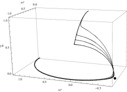
Figure 1: Trajectories in phase space ($x_{\sigma}$, $y_{\sigma}$, $y_{\phi}$) for the potential $V(\sigma,\phi)=V_{0}\sinh^{2}(\alpha\sigma)+V_{1}\cosh^{2}(\beta\phi)$ with ($\alpha$, $\beta$): ($-\sqrt{3}/2$, $0.35$). With this parameter selection the scalar field matter dominated era ($P_{4}$, black point in this graphic) is a saddle, whereas, the phantom field dominated solution ($P_{8}$ in Table 2) is the late time attractor.

Figure 2: Trajectories in phase space ($x_{\sigma}$, $y_{\sigma}$) with the same parameter selection of Fig. 1. The critical point $P_{4}$ represented by the black point is a scalar field matter dominated transient solution.

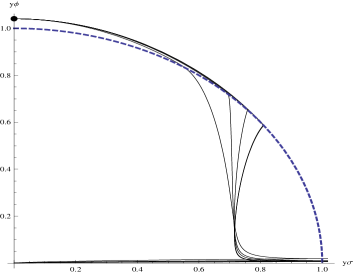
Figure 3: Trajectories in phase space ($y_{\sigma}$, $y_{\phi}$) with the same parameter selection of Fig. 1. The accelerated de Sitter solution $P_{7}$, dashed line, is a transient era in the evolution of the Universe and the late time attractor the phantom field dominated solution, black point in this figure, allowing a crossing through the phantom divide.

V Conclusions

In the present paper a thorough study of the phase space of quintom model has been undertaken. The results are valid for those potential, without interaction between the fields, for which the quantities $\Gamma_{\sigma}=\frac{V_{\sigma}(\sigma)V_{\sigma}^{\prime\prime}(\sigma)}{(V_{\sigma}^{\prime}(\sigma))^{2}}$ and $\Gamma_{\phi}=\frac{V_{\phi}(\phi)V_{\phi}^{\prime\prime}(\phi)}{(V_{\sigma}^{\prime}(\phi))^{2}}$ can be written as a function of the variables $\lambda_{\sigma}$ and $\lambda_{\phi}$.

It has been found that for $g^{\prime}(\lambda_{\phi}^{\ast})\lambda_{\phi}^{\ast}<0$, the late time attractor are always the phantom dominated solution ($P_{8}$) generalizing the result shown in Guo2005 ; Cai2010 for exponential potentials (but more generally, for potential satisfying $\lambda_{\sigma}\approx const$ and $\lambda_{\phi}\approx const$). Otherwise, it is a saddle point. The Universe evolves from a quintessence dominated phase to a phantom dominated phase crossing the $w_{eff}=-1$ divide line as a transient stage Guo2006 .

Center Manifold Theory have been employed to analyze the stability of de Sitter solution either with phantom ($P_{5}$) or quintessence potential dominance ($P_{6}$). After deriving the evolution equation on the center manifolds and making several numerical integrations we have concluded that in both cases the corresponding de Sitter solution is unstable (saddle-like). For $P_{5}$ we have used an analytical argument, whereas for $P_{6}$ our conclusion was supported partially on analytical arguments and complemented by numerical experimentation.

Another important issue is concerning the existence of a point, $P_{4},$ corresponding to the standard quintessence dominated solution, which under certain condition on the potential, can mimick the dark matter behavior. This feature has important cosmological consequences to address de unified description of dark matter and dark energy in a single field. The saddle type character of $P_{4}$ have been clearly illustrated by resorting to phase plane diagrams for the potential obtained from a canonical quantum cosmology.

Appendix A Center manifold dynamics for the solution dominated by the potential energy of the phantom component $P_{5}$

In this section we will shown how we can apply the center manifold theorem to study the stability of non-hyperbolic point $P_{5}$ corresponding to the solution dominated by the potential energy of the phantom component perko2001differential . First, we restrict our attention to the domain $-\frac{3}{4}<g(0)<0$ to dealing with real eigenvalues. The first step is to translate the point $P_{5}$ ($x_{\sigma}=0$, $x_{\phi}=0$ $y_{\sigma}=0$, $\lambda_{\sigma}=\mu$, $\lambda_{\phi}=0$) to the origin, where $\mu$ denotes an arbitrary value for $\lambda_{\sigma}$. The next step is to transform the system to its real Jordan form:

$$\frac{d\textbf{u}}{dN} = Z\textbf{u}+F(\textbf{u},\textbf{v})$$ (27)

$$\frac{d\textbf{v}}{dN} = P\textbf{v}+G(\textbf{u},\textbf{v})$$ (28)

where the square matrices $Z$, $P$ have $2$ zero eigenvalues and $3$ eigenvalues with negative real part, respectively. In order to do that we introduce the new variables:

$$u_{1} = y_{\sigma},$$

$$u_{2} = -\sqrt{\frac{2}{3}}x_{\sigma}f(\mu)-\mu+\lambda_{\sigma},$$

$$v_{1} = \sqrt{\frac{2}{3}}x_{\sigma}f(\mu),$$

$$v_{2} = \frac{2\sqrt{6}g(0)x_{\phi}+\left(\sqrt{12g(0)+9}-3\right)\lambda_{\phi}}{2\sqrt{12g(0)+9}},$$

$$v_{3} = \frac{\left(\sqrt{12g(0)+9}+3\right)\lambda_{\phi}-2\sqrt{6}g(0)x_{\phi}}{2\sqrt{12g(0)+9}}$$ (29)

Using the above transformation, the system (27-28) is given explicitly by:

$${u_{1}}^{\prime}=F_{1}(u_{1},u_{2},v_{1},v_{2},v_{3})$$ (30)

$${u_{2}}^{\prime}=-\frac{3v_{1}(f(\mu+u_{2}+v_{1})-f(\mu))}{f(\mu)}+H(u_{1},u_{2},v_{1},v_{2},v_{3})$$

$$\equiv F_{2}(u_{1},u_{2},v_{1},v_{2},v_{3})$$ (31)

$${v_{1}}^{\prime}=-3v_{1}+G_{1}(u_{1},u_{2},v_{1},v_{2},v_{3})$$ (32)

$${v_{2}}^{\prime}=\frac{1}{2}\left(-\sqrt{12g(0)+9}-3\right)v_{2}+G_{2}(u_{1},u_{2},v_{1},v_{2},v_{3})$$ (33)

$${v_{3}}^{\prime}=\frac{1}{2}\left(\sqrt{12g(0)+9}-3\right)v_{3}+G_{3}(u_{1},u_{2},v_{1},v_{2},v_{3}),$$ (34)

where $f^{\prime}=\frac{df}{dN},$ $F_{1},H,G_{1}$ … $G_{3}$ are homogeneous polynomials in the coordinates $(u_{1},u_{2},v_{1},v_{2},v_{3})$ of degree greater than $2$. Following the standard formalism of the center manifold theory, the coordinates which correspond to the non-zero eigenvalues ($v_{1}$, $v_{2}$, $v_{3}$) can be approximated by the functions:

$$k_{1}(u_{1},u_{2}) =a_{1}u_{1}^{2}+a_{2}u_{1}^{3}+a_{3}u_{1}u_{2}+a_{4}u_{1}^{2}u_{2}+a_{5}u_{2}^{2}+$$

$$+a_{6}u_{1}u_{2}^{2}+a_{7}u_{2}^{3}+...+O(u_{1}^{n},u_{2}^{n})$$ (35)

$$k_{2}(u_{1},u_{2}) =b_{1}u_{1}^{2}+b_{2}u_{1}^{3}+b_{3}u_{1}u_{2}+b_{4}u_{1}^{2}u_{2}+b_{5}u_{2}^{2}+$$

$$+b_{6}u_{1}u_{2}^{2}+b_{7}u_{2}^{3}+...+O(u_{1}^{n},u_{2}^{n})$$ (36)

$$k_{3}(u_{1},u_{2}) =c_{1}u_{1}^{2}+c_{2}u_{1}^{3}+c_{3}u_{1}u_{2}+c_{4}u_{1}^{2}u_{2}+c_{5}u_{2}^{2}+$$

$$+c_{6}u_{1}u_{2}^{2}+c_{7}u_{2}^{3}+...+O(u_{1}^{n},u_{2}^{n})$$ (37)

with this set of functions we can solve, to any $n$ desired degree of accurancy, the quasilinear partial differential equation for the center manifold:

$$Dk(\mathbf{u})\left[Z\mathbf{u}+F(\mathbf{u},k(\mathbf{u}))\right]-Pk(\mathbf{u})-G(\mathbf{u},k(\mathbf{u}))=0$$ (38)

In our case: $Z=\left(\begin{array}[]{cc}0&0\\ 0&0\end{array}\right)$ and

$$P=\left(\begin{array}[]{cccc}-3&0&0\\ 0&\frac{1}{2}\left(-\sqrt{12g(0)+9}-3\right)&0\\ 0&0&\frac{1}{2}\left(\sqrt{12g(0)+9}-3\right)\end{array}\right)$$

$$k(\mathbf{u})=\left(\begin{array}[]{c}k_{1}(u_{1},u_{2})\\ k_{2}(u_{1},u_{2})\\ k_{3}(u_{1},u_{2})\end{array}\right)$$

$$Dk(\mathbf{u})=\left(\begin{array}[]{cc}\frac{\partial k_{1}}{\partial u_{1}}&\frac{\partial k_{1}}{\partial u_{2}}\\ \frac{\partial k_{2}}{\partial u_{1}}&\frac{\partial k_{2}}{\partial u_{2}}\\ \frac{\partial k_{3}}{\partial u_{1}}&\frac{\partial k_{3}}{\partial u_{2}}\end{array}\right)$$

$$G(\mathbf{u},k(\mathbf{u}))=\left(\begin{array}[]{c}G_{1}\left(u_{1},u_{2},k_{1}(u_{1},u_{2}),k_{2}(u_{1},u_{2}),k_{3}(u_{1},u_{2})\right)\\ G_{2}\left(u_{1},u_{2},k_{1}(u_{1},u_{2}),k_{2}(u_{1},u_{2}),k_{3}(u_{1},u_{2})\right)\\ G_{3}\left(u_{1},u_{2},k_{1}(u_{1},u_{2}),k_{2}(u_{1},u_{2}),k_{3}(u_{1},u_{2})\right)\end{array}\right)$$

In order to solve equation (38) we put together $Z$, $P$, $k(u_{1},u_{2})$, $Dk(u_{1},u_{2})$ and $G(u_{1},u_{2},k(u_{1},u_{2})),$ then we equate equal powers of $u_{1}$ and $u_{2}$, and in that way we compute $k(u_{1},u_{2})$. Finally we obtain, in the neighborhood of $P_{5}$, the reduced system:

$${\textbf{u}}^{\prime}=Z\textbf{u}+F(\textbf{u},k(\textbf{u})).$$ (39)

The above procedure applied to equations (30-34) leads to:

$$v_{1}=\frac{1}{3}\mu f(\mu)u_{1}^{2}+\frac{1}{3}f(\mu)u_{1}^{2}u_{2}+O(4);v_{2}=v_{3}=O(4).$$ (40)

Neglecting the fourth order terms, the evolution equations on the center manifold are

$$u_{1}^{\prime} = -\frac{1}{2}\mu^{2}u_{1}^{3}$$ (41)

$$u_{2}^{\prime} = -u_{1}^{2}(\mu+u_{2})f(\mu)-\mu u_{1}^{2}u_{2}f^{\prime}(\mu)$$ (42)

For $\mu f^{\prime}(\mu)+f(\mu)\neq 0,$ the orbit of (41)-(42) passing through $(u_{10},u_{20})$ is given by

$$\frac{u_{1}}{u_{10}}=\frac{1}{\sqrt{1+\mu^{2}u_{10}^{2}N}},\;N\geq 0,$$ (43)

$$u_{2}=\left(\eta(\mu)+u_{20}\right)\left(\frac{u_{1}}{u_{10}}\right)^{\frac{2\left(\mu f^{\prime}(\mu)+f(\mu)\right)}{\mu^{2}}}-\eta(\mu),$$ (44)

where $\eta(\mu)=\frac{\mu f(\mu)}{\mu f^{\prime}(\mu)+f(\mu)}.$ Then, for $f(\mu)+\mu f^{\prime}(\mu)>0,$ the orbits approach the point with coordinates $\left(u_{1}=0,u_{2}=-\eta(\mu)\right)$ when $N\rightarrow+\infty.$ If $f(\mu)+\mu f^{\prime}(\mu)\leq 0,$ then, as $N\rightarrow+\infty,$ $u_{1}$ tends to zero and $u_{2}$ becomes unbounded. Generically, the origin is not approached as $N\rightarrow+\infty,$ unless $\mu f(\mu)=0.$

In the especial case $\mu f^{\prime}(\mu)+f(\mu)=0,$ the system (41)-(42) reduces to

$$u_{1}^{\prime} = -\frac{1}{2}\mu^{2}u_{1}^{3}$$ (45)

$$u_{2}^{\prime} = -\mu f(\mu)u_{1}^{2}.$$ (46)

The orbit of (45)-(46) passing through $(u_{10},u_{20})$ is given by

$$\frac{u_{1}}{u_{10}}=\frac{1}{\sqrt{1+\mu^{2}u_{10}^{2}N}},\;N\geq 0,$$ (47)

$$u_{2}=u_{20}+\ln\left[\frac{u_{1}}{u_{10}}\right]^{\frac{2f(\mu)}{\mu}}.$$ (48)

In this case, $u_{1}$ tends to zero and $u_{2}$ becomes unbounded. Summarizing, for $-\frac{3}{4}<g(0)<0$, $P_{5}$ is unstable.

For $g(0)<-\frac{3}{4},$ there are two complex eigenvalues. In this case, in order to obtain the real Jordan Form, we introduce the new variables

$$V_{2}=\frac{v_{2}+v_{3}}{2},\;V_{3}=\frac{v_{2}-v_{3}}{2i}.$$

Using the above transformation, the system (27-28) is given explicitly by:

$${u_{1}}^{\prime}=\widetilde{F_{1}}(u_{1},u_{2},v_{1},V_{2},V_{3})$$ (49)

$${u_{2}}^{\prime}=\widetilde{F_{2}}(u_{1},u_{2},v_{1},V_{2},V_{3})$$ (50)

$${v_{1}}^{\prime}=-3v_{1}+\widetilde{G_{1}}(u_{1},u_{2},v_{1},V_{2},V_{3})$$ (51)

$${V_{2}}^{\prime}=-\frac{3}{2}V_{2}-\frac{1}{2}\sqrt{-12g(0)-9}V_{3}+\widetilde{G_{2}}(u_{1},u_{2},v_{1},V_{2},V_{3})$$ (52)

$${V_{3}}^{\prime}=-\frac{1}{2}\sqrt{-12g(0)-9}V_{2}-\frac{3}{2}V_{3}+\widetilde{G_{3}}(u_{1},u_{2},v_{1},V_{2},V_{3})$$ (53)

where $\widetilde{F_{1}},\widetilde{G_{1}}$ … $\widetilde{G_{3}}$ are homogeneous real polynomials in the coordinates $(u_{1},u_{2},v_{1},V_{2},V_{3})$ of degree greater than $2$. Usig the same procedure as before we obtain that the center manifold is given locally by the graph

$$v_{1}=\frac{1}{3}af(a)u_{1}^{2}+\frac{1}{3}f(a)u_{1}^{2}u_{2}+O(4);V_{2}=V_{3}=O(4).$$ (54)

Thus the dynamics on the center manifold is given by the system (41)-(42) analyzed before. Sumarizing, for $g(0)<0$, $P_{5}$ is unstable.

Appendix B Center manifold dynamics for the solution dominated by the potential energy of the quintessence component $P_{6}$

In this section we will shown how we can apply the center manifold theorem to study the stability of non-hyperbolic point $P_{6}$ corresponding to the solution dominated by the potential energy of the quintessence component perko2001differential .

The first step is to translate the point $P_{6}$ ($x_{\sigma}=0$, $x_{\phi}=0$ $y_{\sigma}=1$, $\lambda_{\sigma}=0$, $\lambda_{\phi}=\mu$) to the origin, where $\mu$ denotes an arbitrary value for $\lambda_{\phi}$. The next step is to transform the system to its real Jordan form:

$$\dot{\textbf{u}} = Z\textbf{u}+F(\textbf{u},\textbf{v})$$ (55)

$$\dot{\textbf{v}} = P\textbf{v}+G(\textbf{u},\textbf{v})$$ (56)

where the square matrices $Z$, $P$ have $2$ zero eigenvalues and $3$ eigenvalues with negative real part, respectively. In order to do that we introduce the new variables:

$$u_{1} = -2\mu(y_{\sigma}-1)g(\mu),$$

$$u_{2} = -\frac{1}{3}g(\mu)\left(\sqrt{6}x_{\phi}-2\mu(y_{\sigma}-1)\right)-\mu+\lambda_{\phi},$$

$$v_{1} = \frac{1}{3}g(\mu)\left(\sqrt{6}x_{\phi}-2\mu(y_{\sigma}-1)\right),$$

$$v_{2} = \frac{2\sqrt{6}f(0)x_{\sigma}+\left(\sqrt{9-12f(0)}-3\right)\lambda_{\sigma}}{2\sqrt{9-12f(0)}},$$

$$v_{3} = \frac{-2\sqrt{6}f(0)x_{\sigma}+\left(\sqrt{9-12f(0)}+3\right)\lambda_{\sigma}}{2\sqrt{9-12f(0)}}.$$ (57)

Using the above transformation, the system (55-56) is given explicitly by:

$${u_{1}}^{\prime}=F_{1}(u_{1},u_{2},v_{1},v_{2},v_{3})$$ (58)

$${u_{2}}^{\prime}=-\frac{3v_{1}(g(\mu+u_{2}+v_{1})-g(\mu))}{g(\mu)}+\frac{u_{1}g(\mu+u_{2}+v_{1})}{g(\mu)}$$

$$+H(u_{1},u_{2},v_{1},v_{2},v_{3})\equiv F_{2}(u_{1},u_{2},v_{1},v_{2},v_{3})$$ (59)

$${v_{1}}^{\prime}=-3v_{1}+G_{1}(u_{1},u_{2},v_{1},v_{2},v_{3})$$ (60)

$${v_{2}}^{\prime}=\frac{1}{2}\left(-\sqrt{9-12f(0)}-3\right)v_{2}+G_{2}(u_{1},u_{2},v_{1},v_{2},v_{3})$$ (61)

$${v_{3}}^{\prime}=\frac{1}{2}\left(\sqrt{9-12f(0)}-3\right)v_{3}+G_{3}(u_{1},u_{2},v_{1},v_{2},v_{3})$$ (62)

near the non-hyperbolic fixed point $P_{6}$ where $F_{1},H,G_{1}$ … $G_{3}$ are homogeneous polynomials in the coordinates $(u_{1},u_{2},v_{1},v_{2},v_{3})$ of degree greater than $2$. Following the standard formalism of the center manifold theory, we obtain that the center manifold of $P_{6}$ is given by the graph

$$v_{1}=\frac{\mu u_{1}^{2}}{18g(\mu)}+\frac{u_{1}^{2}}{12\mu g(\mu)}+\frac{u_{1}^{2}}{9\mu}-\frac{u_{1}u_{2}}{3\mu}+O(3);$$

$$v_{2}=O(3),v_{3}=O(3).$$ (63)

Neglecting the third order terms, the evolution equations on the center manifold are

$$u_{1}^{\prime} = \frac{\mu u_{1}^{2}}{g(\mu)}$$ (64)

$$u_{2}^{\prime} = \frac{u_{1}u_{2}}{\mu}-\frac{\left(2\mu^{2}+3\right)u_{1}^{2}}{12\mu g(\mu)}$$ (65)

Let us assume $g(\mu)\neq 0,\mu\neq 0.$ Hence, the orbit of (64)-(65) passing through $(u_{10},u_{20})$ is given by

$$u_{2}=\frac{\left(\left(2\mu^{2}+3\right)u_{10}+12\mu^{2}u_{20}-12u_{20}g(\mu)\right)}{12\left(\mu^{2}-g(\mu)\right)}\left(\frac{u_{1}}{u_{10}}\right)^{\frac{g(\mu)}{\mu^{2}}}+$$

$$+\frac{\left(2\mu^{2}+3\right)u_{1}}{12\left(g(\mu)-\mu^{2}\right)},$$ (66)

$$\frac{u_{1}}{u_{10}}=\frac{g(\mu)}{g(\mu)-\mu u_{10}N},\;N\geq 0,$$ (67)

In order to investigate the stability of the center manifold of $P_{6}$ we have resorted to several numerical integrations of the system (64)-(65). We find four typical situations that suggest that $P_{6}$ is unstable (saddle type).

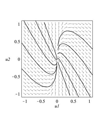
Figure 4: Vector field in the plane ($u_{1}$, $u_{2}$) for the potential $V(\sigma,\phi)=V_{0}\sinh^{2}(\alpha\sigma)+V_{1}\cosh^{2}(\beta\phi)$. The free parameter have been chosen to be ($\alpha$, $\beta$, $\mu$): ($-\sqrt{3}/2$, $0.35$, $0.50$). In this case $g(\mu)=0.12>0$. The sign of $u_{1}$ is invariant. For $u_{1}<0$ the origin is approached as the time goes forward whereas for $u_{1}>0$ the orbits departs from the origin. Thus, the accelerated de Sitter solution $P_{6}$ is a transient era in the evolution of the Universe.

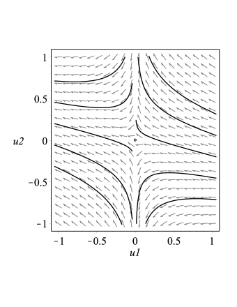
Figure 5: Vector field in the plane ($u_{1}$, $u_{2}$) for the potential $V(\sigma,\phi)=V_{0}\sinh^{2}(\alpha\sigma)+V_{1}\cosh^{2}(\beta\phi)$. The free parameter have been chosen to be ($\alpha$, $\beta$, $\mu$): ($-\sqrt{3}/2$, $0.35$, $1.30$). In this case $g(\mu)=-0.60<0$. The origin is of saddle type. Thus the accelerated de Sitter solution $P_{6}$ is a transient era in the evolution of the Universe.

In the figure 4 is displayed the vector field in the plane ($u_{1}$, $u_{2}$) for the potential $V(\sigma,\phi)=V_{0}\sinh^{2}(\alpha\sigma)+V_{1}\cosh^{2}(\beta\phi)$. The free parameter have been chosen to be ($\alpha$, $\beta$, $\mu$): ($-\sqrt{3}/2$, $0.35$, $0.50$). In this case $g(\mu)=0.12>0$. The sign of $u_{1}$ is invariant. For $u_{1}<0$ the origin is approached as the time goes forward whereas for $u_{1}>0$ the orbits departs form the origin. For the choice ($\alpha$, $\beta$, $\mu$): ($-\sqrt{3}/2$, $0.35$, $-0.50$). we have $g(\mu)=0.12>0$. The figure is similar to 4 with the arrows in reverse orientation. Thus, this numerical elaboration suggest that the accelerated de Sitter solution $P_{6}$, (the origin of coordinates), is a transient era in the evolution of the Universe for $g(\mu)>0$ irrespectively the sign of $\mu$.

In the figure 5 is represented the vector field in the plane ($u_{1}$, $u_{2}$) for the potential $V(\sigma,\phi)=V_{0}\sinh^{2}(\alpha\sigma)+V_{1}\cosh^{2}(\beta\phi)$. The free parameter have been chosen to be ($\alpha$, $\beta$, $\mu$): ($-\sqrt{3}/2$, $0.35$, $1.30$). In this case $g(\mu)=-0.60<0$. The sign of $u_{1}$ is invariant. All the orbits departs from the origin. Thus the accelerated de Sitter solution $P_{6}$ is a transient era in the evolution of the Universe. For the choice ($\alpha$, $\beta$, $\mu$): ($-\sqrt{3}/2$, $0.35$, $-0.30$). we have $g(\mu)=0.20>0$. The figure is similar to 4 with the arrows in reverse orientation. Thus, this numerical elaboration suggest that the accelerated de Sitter solution $P_{6}$, is a transient era in the evolution of the Universe for $g(\mu)<0$ irrespectively the sign of $\mu$.

As in the appendix A, for analyzing the case of complex eigenvalues, we can introduce the new variables

$$V_{2}=\frac{v_{2}+v_{3}}{2},\;V_{3}=\frac{v_{2}-v_{3}}{2i}$$

for deriving the real Jordan form of the Jacobian. The procedure is straightforward, so we won’t enter into the details here.

References

• [1] Adam G. Riess, Lucas Macri, Stefano Casertano, Hubert Lampeitl, Henry C. Ferguson, et al. A 3Space Telescope and Wide Field Camera 3. Astrophys.J., 730:119, 2011.
• [2] E. Komatsu et al. Seven-Year Wilkinson Microwave Anisotropy Probe (WMAP) Observations: Cosmological Interpretation. Astrophys.J.Suppl., 192:18, 2011.
• [3] Beth A. Reid, Will J. Percival, Daniel J. Eisenstein, Licia Verde, David N. Spergel, et al. Cosmological Constraints from the Clustering of the Sloan Digital Sky Survey DR7 Luminous Red Galaxies. Mon.Not.Roy.Astron.Soc., 404:60–85, 2010.
• [4] Hong Li and Xin Zhang. Probing the dynamics of dark energy with divergence-free parametrizations: A global fit study. Phys.Lett., B703:119–123, 2011.
• [5] Ujjaini Alam, Varun Sahni, and A.A. Starobinsky. The Case for dynamical dark energy revisited. JCAP, 0406:008, 2004.
• [6] Bo Feng, Xiu-Lian Wang, and Xin-Min Zhang. Dark energy constraints from the cosmic age and supernova. Phys.Lett., B607:35–41, 2005.
• [7] Dragan Huterer and Asantha Cooray. Uncorrelated estimates of dark energy evolution. Phys.Rev., D71:023506, 2005.
• [8] S. Nesseris and Leandros Perivolaropoulos. Crossing the Phantom Divide: Theoretical Implications and Observational Status. JCAP, 0701:018, 2007.
• [9] Harvinder K. Jassal, J.S. Bagla, and T. Padmanabhan. Understanding the origin of CMB constraints on Dark Energy. Mon.Not.Roy.Astron.Soc., 405:2639–2650, 2010.
• [10] Bohdan Novosyadlyj, Olga Sergijenko, Ruth Durrer, and Volodymyr Pelykh. Do the cosmological observational data prefer phantom dark energy? Phys.Rev., D86:083008, 2012.
• [11] B. Novosyadlyj, O. Sergijenko, R. Durrer, and V. Pelykh. Quintessence versus phantom dark energy: the arbitrating power of current and future observations. 2012.
• [12] G. Hinshaw, D. Larson, E. Komatsu, D.N. Spergel, C.L. Bennett, et al. Nine-Year Wilkinson Microwave Anisotropy Probe (WMAP) Observations: Cosmological Parameter Results. 2012.
• [13] Alexander Vikman. Can dark energy evolve to the phantom? Phys.Rev., D71:023515, 2005.
• [14] Wayne Hu. Crossing the phantom divide: Dark energy internal degrees of freedom. Phys.Rev., D71:047301, 2005.
• [15] Robert R. Caldwell and Michael Doran. Dark-energy evolution across the cosmological-constant boundary. Phys.Rev., D72:043527, 2005.
• [16] Jun-Qing Xia, Yi-Fu Cai, Tao-Tao Qiu, Gong-Bo Zhao, and Xinmin Zhang. Constraints on the Sound Speed of Dynamical Dark Energy. Int.J.Mod.Phys., D17:1229–1243, 2008.
• [17] Yi-Fu Cai, Emmanuel N. Saridakis, Mohammad R. Setare, and Jun-Qing Xia. Quintom Cosmology: Theoretical implications and observations. Phys.Rept., 493:1–60, 2010.
• [18] Cedric Deffayet, Oriol Pujolas, Ignacy Sawicki, and Alexander Vikman. Imperfect Dark Energy from Kinetic Gravity Braiding. JCAP, 1010:026, 2010.
• [19] Xiao-Fei Zhang, Hong Li, Yun-Song Piao, and Xin-Min Zhang. Two-field models of dark energy with equation of state across -1. Mod.Phys.Lett., A21:231–242, 2006.
• [20] Zong-Kuan Guo, Yun-Song Piao, Xin-Min Zhang, and Yuan-Zhong Zhang. Cosmological evolution of a quintom model of dark energy. Phys.Lett., B608:177–182, 2005.
• [21] Ruth Lazkoz and Genly Leon. Quintom cosmologies admitting either tracking or phantom attractors. Phys.Lett., B638:303–309, 2006.
• [22] Ruth Lazkoz, Genly Leon, and Israel Quiros. Quintom cosmologies with arbitrary potentials. Phys.Lett., B649:103–110, 2007.
• [23] M.R. Setare and E.N. Saridakis. Quintom Cosmology with General Potentials. Int.J.Mod.Phys., D18:549–557, 2009.
• [24] M.R. Setare and E.N. Saridakis. Quintom model with O(N) symmetry. JCAP, 0809:026, 2008.
• [25] M.R. Setare and E.N. Saridakis. Quintom dark energy models with nearly flat potentials. Phys.Rev., D79:043005, 2009.
• [26] W. Guzman, M. Sabido, J. Socorro, and L. Arturo Urena-Lopez. Scalar potentials out of canonical quantum cosmology. Int.J.Mod.Phys., D16:641–654, 2007.
• [27] J. Socorro and Marco D’Oleire. Inflation from Supersymmetric Quantum Cosmology. Phys.Rev., D82:044008, 2010.
• [28] David Bohm. A Suggested interpretation of the quantum theory in terms of hidden variables. 1. Phys.Rev., 85:166–179, 1952.
• [29] Wei Fang, Ying Li, Kai Zhang, and Hui-Qing Lu. Exact Analysis of Scaling and Dominant Attractors Beyond the Exponential Potential. Class.Quant.Grav., 26:155005, 2009.
• [30] Yoelsy Leyva, Dania Gonzalez, Tame Gonzalez, Tonatiuh Matos, and Israel Quiros. Dynamics of a self-interacting scalar field trapped in the braneworld for a wide variety of self-interaction potentials. Phys.Rev., D80:044026, 2009.
• [31] Dagoberto Escobar, Carlos R. Fadragas, Genly Leon, and Yoelsy Leyva. Phase space analysis of quintessence fields trapped in a Randall-Sundrum Braneworld: anisotropic Bianchi I brane with a Positive Dark Radiation term. Class.Quant.Grav., 29:175006, 2012.
• [32] Dagoberto Escobar, Carlos R. Fadragas, Genly Leon, and Yoelsy Leyva. Phase space analysis of quintessence fields trapped in a Randall-Sundrum Braneworld: a refined study. Class.Quant.Grav., 29:175005, 2012.
• [33] Tonatiuh Matos, Jose-Ruben Luevano, Israel Quiros, L. Arturo Urena-Lopez, and Jose Alberto Vazquez. Dynamics of Scalar Field Dark Matter With a Cosh-like Potential. Phys.Rev., D80:123521, 2009.
• [34] Israel Quiros, Tame Gonzalez, Dania Gonzalez, and Yunelsy Napoles. Study Of Tachyon Dynamics For Broad Classes of Potentials. Class.Quant.Grav., 27:215021, 2010.
• [35] Wei Fang and Hui-Qing Lu. Dynamics of tachyon and phantom field beyond the inverse square potentials. Eur.Phys.J., C68:567–572, 2010.
• [36] H. Farajollahi, A. Salehi, F. Tayebi, and A. Ravanpak. Stability Analysis in Tachyonic Potential Chameleon cosmology. JCAP, 1105:017, 2011.
• [37] Kui Xiao and Jian-Yang Zhu. Stability analysis of an autonomous system in loop quantum cosmology. Phys.Rev., D83:083501, 2011.
• [38] Edmund J. Copeland, Andrew R Liddle, and David Wands. Exponential potentials and cosmological scaling solutions. Phys.Rev., D57:4686–4690, 1998.
• [39] Xi-ming Chen, Yun-gui Gong, and Emmanuel N. Saridakis. Phase-space analysis of interacting phantom cosmology. JCAP, 0904:001, 2009.
• [40] Zong-Kuan Guo, Yun-Song Piao, Xinmin Zhang, and Yuan-Zhong Zhang. Two-Field Quintom Models in the w-w’ Plane. Phys.Rev., D74:127304, 2006.
• [41] L. Perko. Differential Equations and Dynamical Systems. Texts in Applied Mathematics. Springer, 2001.