Quantum computation by local measurement

Abstract: Quantum computation is a novel way of information processing which allows, for certain classes of problems, exponential speedups over classical computation. Various models of quantum computation exist, such as the adiabatic, circuit and measurement-based models. They have been proven equivalent in their computational power, but operate very differently. As such, they may be suitable for realization in different physical systems, and also offer different perspectives on open questions such as the precise origin of the quantum speedup. Here, we give an introduction to the one-way quantum computer, a scheme of measurement-based quantum computation. In this model, the computation is driven by local measurements on a carefully chosen, highly entangled state. We discuss various aspects of this computational scheme, such as the role of entanglement and quantum correlations. We also give examples for ground states of simple Hamiltonians which enable universal quantum computation by local measurements.

1 Introduction

Quantum computation is a promising approach to harness the laws of quantum mechanics for solving computational problems. A particular striking example is Shor’s efficient quantum algorithm for factoring large numbers [1], which breaks the RSA crypto system. After this splendid start, the growing field has encountered numerous challenges, some of which it has mastered, some of which it still faces. As an example, decoherence was initially conceived as an insurmountable obstacle to scalable quantum computation [2]. However, the theory of quantum-error correction [3]-[7] and, alternatively, the scheme of topological quantum computation [8, 9], show that it can in principle be overcome. Also, impressive experimental progress has been made in recent years towards realizing quantum computers in the laboratory [10]-[19]. Yet, building a large-scale device in the foreseeable future remains a great challenge [20].

At a fundamental level, we may ask “Which quantum mechanical property is responsible for the quantum speedup?” In spite of a number of candidates that have been proposed—such as entanglement, superposition and interference, and largeness of Hilbert space—we have no rigorous and generally applicable answer to this question yet. Making progress in this direction may, in addition to deepening our understanding of quantum computation, also lay the foundation for the design of novel quantum algorithms. In 1948, introducing the path integral formalism to quantum mechanics [21], Richard Feynman wrote: “One feels like Cavalieri must have felt calculating the volume of a pyramid before the invention of calculus.” Addressing the above questions in the theory of quantum computation feels like that, too.

The paradigm of measurement-based quantum computation (MBQC), with the teleportation-based schemes [22] and the one-way quantum computer [23, 24, 25] as the most prominent examples, offers a new framework within which both theoretical and experimental challenges of quantum computation can be addressed. This article focuses on the one-way quantum computer, in which the measurements driving the computation are strictly local. We will discuss its prospects for experimental realization, and examine the roles that entanglement and quantum correlations play for it.

In the one-way MBQC, the process of computation is driven solely by local measurements, applied to a highly entangled resource state. This is in stark contrast to the (standard) circuit model, where the quantum is driven by elementary steps of unitary evolution, so-called quantum gates. In the MBQC, after a highly entangled resource state such as a 2D cluster state [26] has been created, the local systems, say qubits, are measured individually in certain bases and a prescribed temporal order. The choice of measurement bases specifies which quantum algorithm is being implemented. The measurement outcomes cannot be chosen; they are individually random. This randomness can be prevented from creeping into the logical processing by adjusting measurement bases according to previously obtained measurement outcomes. Finally, the computational output is produced by correlations of measurement outcomes.

The remainder of this article is dedicated to a few questions that arise at this point. (i) Is MBQC experimentally feasible? - We discuss pro’s and con’s for the experimental realization of MBQC in Section 2. (ii) Why does MBQC work at all? - We provide an explanation of the inner workings of MBQC in Section 3. (iii) Do resource states for universal MBQC arise naturally in quantum systems? - In Section 3.1, we describe how a particular universal resource state, the cluster state, can be realized via unitary evolution under an Ising Hamiltonian. In Section 3.2, we explain teleportation-based implementations of quantum gates. Building on that, in Section 3.3, we explain how a CNOT gate and general one-qubit rotations can be realized using cluster states, leading to universality of MBQC. Section 4 describes how computational resources can arise as ground states of relatively simple Hamiltonians. A resource for universal MBQC is the Affleck-Kennedy-Lieb-Tasaki state on the honeycomb lattice; see Section 4.2. (iv) Which role does entanglement play for MBQC? - In MBQC, the result of the computation is obtained at the price of consuming all or most of the entanglement initially present in the resource state. Therefore, entanglement appears as a key resource for MBQC. In Section 5.1, this intuition is (partially) corroborated, and in Section 5.2 its limits are shown. (v) Which role do quantum correlations play for MBQC? The computational power of MBQC hinges on strong correlations among the random measurement outcomes. These classical correlations derive from quantum correlations in the resource state. In Section 6, we illustrate this in a specific example, by turning the Greenberger-Horne-Zeilinger proof of Bell’s theorem into a measurement-based quantum computation.

Figure 1: Quantum computation by measuring individual qubits initially prepared in a cluster state on a two-dimensional lattice, circuit simulator view. The choice of measurement bases specifies the sequence of simulated quantum gates. Circles symbolize measurements of $\sigma_{z}$, and arrows refer to measurement bases in the x-y plane.

2 Prospects for realization of scalable MBQC

Physical systems considered for realizing a quantum computer have to meet a set of requirements, known as the DiVincenzo criteria. Specifically, one requires (i) A scalable setup with well-defined qubits, (ii) The ability to initialize the qubits in a fiducial state, say $|00..0\rangle$, (iii) A universal set of quantum gates, (iv) The ability to measure individual qubits, and (v) Long coherence times. For various potential realizations of a quantum computer, such as trapped ions [13]-[16], lattices of cold atoms [11, 12], photons [17] and superconducting qubits [18], at least a subset of the DiVincenzo criteria have been proven in the experiment. It can be expected that these physical systems will mature into medium-scale test beds for quantum computers over the next couple of years, but it is far from certain that which one of them will emerge as the quantum counterpart of the silicon chip.

The scheme of measurement-based quantum computation can simplify the architecture of a quantum computer since it reduces the requirements on the interaction between qubits. First, instead of tunable interactions between selected pairs of qubits, MBQC only requires a translation-invariant, nearest-neighbor Ising coupling. This interaction is highly scalable and parallelized, and requires no control other than an on/off switch.

Physical systems that can naturally make use of this advantage are optical lattices filled with cold atoms. In recent years, substantial experimental progress has been made in trapping, cooling and manipulating cold atoms in optical lattices. Large areas in such a lattice can be regularly filled with one atomic qubit per site, by driving a superfluid to Mott phase transition [27]. Furthermore, the Ising interaction can be realized by cold controlled collisions between the atoms [11]. Finally, the extremely difficult single site readout has recently been experimentally demonstrated [28].

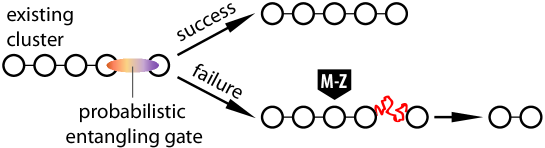
A second setting in which MBQC helps to overcome a limitation of the interaction are probabilistic heralded entangling gates. In this setting, the entangling gate sometimes (or mostly) fails but success is confirmed by a classical signal. The problem with using probabilistic gates in quantum circuits in the same way as deterministic ones is that a single failed gate ruins the entire computation. Instead, probabilistic heralded entangling gates may be used to grow a cluster state. A simple protocol for probabilistic growth of a linear cluster state is depicted in Fig. 2. It works whenever the success probability of the heralded entangling gate is greater than 2/3. This protocol can be refined. It turns out that cluster states of arbitrary size and geometry can be grown efficiently for any success probability $p>0$ of the entangling gate, enabling universal computation [29, 30].

Figure 2: Simple method for probabilistic growth of cluster states. A probabilistic heralded conditional phase gate ($\mbox{cPhase}_{ij}:=\exp(i\pi|11\rangle_{ij}\langle 11|)$) is applied to an existing linear cluster state. If the gate succeeds, the length of the cluster is increased by one. If the gate fails, the cluster qubit next to the qubits affected by the failed gate is measured in the $\sigma_{z}$-eigenbasis, recovering the cluster to the left. The length of the cluster is reduced by two. On average, the cluster grows if the success probability of the entangling gate is $>2/3$.

A physical setting where probabilistic heralded entangling gates arise naturally is the Knill-Laflamme-Milburn (KLM) scheme of linear optics quantum computation [31]. Probabilistic growth of cluster states can be gainfully applied in this setting. Specifically, it reduces the operational overhead from a factor that grows with the size of the computation to a constant factor [32, 33]. See [34] for a similar result within teleportation-based quantum computation [22]. Readers interested in knowing more detail about how MBQC helps to reduce the resource in KLM scheme beyond the explanation in Fig. 2 should refer to the above cited works.

MBQC also has a disadvantage for the realization of quantum computation. As a glance at Fig. 1 reveals, the number of qubits that need to be stored simultaneously is significantly increased as compared to the circuit model. Note, however, that the cluster state can be continuously created ‘on the fly’, mitigating this effect.

Finally, it shall be noted that MBQC has been realized on a small scale in an experiment with photons [17]. There, a four-qubit cluster state was created and subsequently measured, allowing for the realization of Grover search [35] on a four-item data base.

3 How MBQC works

In this section we show that a measurement-based quantum computer has the full power of quantum computation, by mapping to the (standard) circuit model.

To establish this result, we regard MBQC as a circuit simulator. In this view, the cluster state provides a ‘canvas’ upon which a quantum circuit is imprinted by local measurements. One spatial direction of the cluster, the vertical direction, say, labels the positions of logical qubits on a line. The perpendicular direction corresponds to the circuit time. As the measurements progress from left to right, the logical qubits are propagated across the cluster slice by slice, implementing quantum gates in the passing.

We assume familiarity with elementary notions of the circuit model, such as the quantum register, quantum gates and quantum circuits [39]. In short, a quantum circuit begins with the initialization of an $n$-qubit quantum register in a fixed state such as $|00...0\rangle$. Second, a sequence of unitary quantum gates is applied. Third, the qubits of the quantum register are individually measured in a fixed basis, and the readout of the computation is thereby obtained.

3.1 Cluster states

Of central importance for MBQC is the choice of the initial resource state. For sure, this state has to be entangled, but not every entangled state will do. In fact, MBQC resource states that allow for universal quantum computation by local measurement are extremely rare [36, 37], and only a small number of such states are known explicitly.

The first universal resource state to be discovered was the two-dimensional cluster state, which we introduce here by a practical two-step procedure to create it. Consider a two-dimensional lattice ${\cal{L}}_{2}$, with one qubit located at each site $a\in V({\cal{L}}_{2})$, the set of vertices, and with an edge set $E({\cal{L}}_{2})$, where an $e$ in $E({\cal L}_{2})$ denotes a pair of distinct vertices, e.g., $(i,j)$, that are interacting with each other. Then, a 2D cluster state $|\phi\rangle_{{\cal{L}}_{2}}$ is created by (i) preparing the qubits $a\in V({\cal{L}}_{2})$ individually in the state $|+\rangle_{a}=1/\sqrt{2}(|0\rangle_{a}+|1\rangle_{a})$, and (ii) unitarily evolving this state under the Ising-like Hamiltonian

$$H({\cal{L}}_{2})=\hbar g\sum_{(i,j)\in E({\cal{L}}_{2})}\frac{I^{(i)}-\sigma_{z}^{(i)}}{2}\otimes\frac{I^{(j)}-\sigma_{z}^{(j)}}{2}=\hbar g\sum_{(i,j)\in E({\cal{L}}_{2})}|1\rangle_{i}\langle 1|\otimes|1\rangle_{j}\langle 1|,$$ (1)

for a time $T=\pi/g$. Equivalently,

$$|\phi\rangle_{{\cal{L}}_{2}}=\prod_{(a,b)\in E({\cal{L}}_{2})}\mbox{cPhase}_{a,b}\,\bigotimes_{a\in V({\cal{L}}_{2})}|+\rangle_{a}.$$ (2)

Therein, $\mbox{cPhase}_{c,t}:=\exp\left(i\pi|11\rangle_{c,t}\langle 11|\right)=\mbox{cPhase}_{t,c}$ is a unitary quantum gate, a so-called conditional phase gate, a.k.a. control-phase gate, which is symmetric w.r.t. to the control (c) and target (t) qubits. One can also rewrite the conditional phase gate in a useful representation

$$\mbox{cPhase}_{c,t}=|0\rangle_{c}\langle 0|\otimes I_{t}+|1\rangle_{c}\langle 1|\otimes Z_{t},$$ (3)

which only flips the phase of the target qubit when the control qubit is in the state $|1\rangle$. The conditional phase gates on the r.h.s. of Eq. (2) commute, so that their temporal ordering is immaterial.

The control-phase gate can be shown to satisfy the following properties

$$\begin{array}[]{rcl}\mbox{cPhase}_{a,b}\,X_{a}\,\mbox{cPhase}_{a,b}^{\dagger}&=&X_{a}Z_{b},\\ \mbox{cPhase}_{a,b}\,X_{b}\,\mbox{cPhase}_{a,b}^{\dagger}&=&X_{b}Z_{a},\\ \mbox{cPhase}_{a,b}\,Z_{a}\,\mbox{cPhase}_{a,b}^{\dagger}&=&Z_{a},\\ \mbox{cPhase}_{a,b}\,Z_{b}\,\mbox{cPhase}_{a,b}^{\dagger}&=&Z_{b},\end{array}$$ (4)

where, for convenience, we have used $X$, $Y$, and $Z$ to denote the Pauli matrices $\sigma_{x}$, $\sigma_{y}$, and $\sigma_{z}$, respectively. Using the above equations, we can show that

$$\prod_{(i,j)\in E({\cal L}_{2})}{\rm cPhase}_{i,j}\,X_{u}=\Big{(}X_{u}\prod_{v\in{\rm Nb}(u)}Z_{v}\Big{)}\prod_{(i,j)\in E({\cal L}_{2})}{\rm cPhase}_{i,j},$$ (5)

where ${\rm Nb}(u)$ denotes the set of vertices that are neighbors of $u$. Applying this relation to an initial state $|+\rangle|+\rangle\cdots|+\rangle$, we arrive at

$$\Big{(}X_{u}\prod_{v\in{\rm Nb}(u)}Z_{v}\Big{)}|\phi\rangle_{{\cal L}_{2}}=|\phi\rangle_{{\cal L}_{2}},\;\;\forall u\in V({\cal{L}}_{2}).$$ (6)

Eq. (6) uniquely specifies the cluster state $|\phi\rangle$ given the graph ${\cal L}_{2}$, and is thus equivalent to Eq. (2) as a definition for cluster states. It has the advantage of being independent of any particular creation procedure.

Cluster states are special cases of a slightly more general class of states, the graph states. We now define graph states in a way similar to Eq. (6).

Definition 1 (Graph states and cluster states).

Consider a graph $G$ with vertex set $V(G)$ and edge set $E(G)$, and a set of qubits, one for each vertex $a\in V(G)$. The graph state $|G\rangle$ is the unique simultaneous eigenstate with eigenvalue 1 of the Pauli operators

$$K_{a}=X_{a}\bigotimes_{b\in{\rm Nb}(a)\in E(G)}Z_{b},\;\;\;\;\forall a\in V(G),$$ (7)

i.e., $|G\rangle=K_{a}|G\rangle$ for all $a\in V(G)$. Therein, $X\equiv\sigma_{x}=|0\rangle\langle 1|+|1\rangle\langle 0|$ and $Z\equiv\sigma_{z}=|0\rangle\langle 0|-|1\rangle\langle 1|$.

A cluster state $|\phi\rangle_{\cal{L}}$ is a graph state with the corresponding graph being a lattice ${\cal{L}}$ of some dimension $d$, $|\phi\rangle_{\cal{L}}:=|{\cal{L}}\rangle$.

Let us now consider two examples of one-dimensional cluster states. Example I: The two-qubit cluster state $|\phi_{2}\rangle$. From the first definition Eq. (2), using $\mbox{cPhase}_{i,j}:=\exp(i\pi|11\rangle_{ij}\langle 11|)=|0\rangle_{i}\langle 0|\otimes I^{(j)}+|1\rangle_{i}\langle 1|\otimes Z^{(j)}$, we have

$$|\phi_{2}\rangle={\rm cPhase}_{12}|+\rangle_{1}|+\rangle_{2}=\frac{1}{\sqrt{2}}{\rm cPhase}_{12}(|0\rangle_{1}+|1\rangle_{1})|+\rangle_{2}=\frac{|0\rangle_{1}|+\rangle_{2}+|1\rangle_{1}|-\rangle_{2}}{\sqrt{2}},$$ (8)

where we have expanded the first qubit in $|0/1\rangle$ basis and used the relation $Z|\pm\rangle=|\mp\rangle$ to flip the phase of the second qubit. Although both the initial state and the conditional phase gate are symmetric w.r.t. qubits 1 and 2, the final state does not explicitly show this symmetry in the given basis. One may as well use the second qubit as the control and the first qubit as the target and redo the calculation,

$$|\phi_{2}\rangle={\rm cPhase}_{21}|+\rangle_{1}|+\rangle_{2}=\frac{1}{\sqrt{2}}{\rm cPhase}_{21}|+\rangle_{1}(|0\rangle_{2}+|1\rangle_{2})=\frac{|+\rangle_{1}|0\rangle_{2}+|-\rangle_{1}|1\rangle_{2}}{\sqrt{2}}.$$ (9)

The second definition Eq. (7) of the cluster state $|\phi_{2}\rangle$ yields the relations $X_{1}Z_{2}|\phi_{2}\rangle=Z_{1}X_{2}|\phi_{2}\rangle=|\phi_{2}\rangle$. We can now explicitly verify that the state on the r.h.s. of Eq. (8), as well as Eq. (9), satisfies these two relations.

Example II: The three-qubit cluster state $|\phi_{3}\rangle$ on a line. Defined through Eq. (2), it takes the form

$$|\phi_{3}\rangle={\rm cPhase}_{23}\,{\rm cPhase}_{21}|+\rangle_{1}|+\rangle_{2}|+\rangle_{3}={\rm cPhase}_{23}|\phi_{2}\rangle|+\rangle_{3}=\frac{|+\rangle_{1}|0\rangle_{2}|+\rangle_{3}+|-\rangle_{1}|1\rangle_{2}|-\rangle_{3}}{\sqrt{2}}$$ (10)

Notice that we have used the second form of $|\phi_{2}\rangle$ (9), indicated by the labeling of the conditional phase gate ${\rm cPhase}_{21}$, as then the second qubit is in the $|0/1\rangle$ basis, convenient for the subsequent gate ${\rm cPhase}_{23}$. Eq. (6) yields an implicit but equivalent definition, through the stabilizer equations $X_{1}Z_{2}\,|\phi_{3}\rangle=|\phi_{3}\rangle$, $Z_{1}X_{2}Z_{3}\,|\phi_{3}\rangle=|\phi_{3}\rangle$, $Z_{2}X_{3}\,|\phi_{3}\rangle=|\phi_{3}\rangle$. Again, these relations can be explicitly verified for the state on the r.h.s. of Eq. (10). Note that if we attach to $|\phi_{3}\rangle$ a fourth qubit in $|+\rangle_{4}$ and apply ${\rm cPhase}_{43}$ we obtain the linear four-qubit cluster state $|\phi_{4}\rangle$, and we can continue this procedure for any linear cluster state. The number of terms needed to describe the cluster state grows exponentially in the number of qubits. Indeed, it doubles upon adding two more qubits into the chain.

From the stabilizer relations follows, for example, that if qubits 1 and 3 are measured in the $Z$-basis and qubit 2 is measured in the $X$-basis, then the measured eigenvalues $\lambda_{Z}^{(1)},\lambda_{X}^{(2)},\lambda_{Z}^{(3)}\in\{1,-1\}$ are individually random but correlated, with $\lambda_{Z}^{(1)}\lambda_{X}^{(2)}\lambda_{Z}^{(3)}=1$. In MBQC, output bits of the computation will be inferred from correlations like this one, but generally in more complicated bases. We note that $|\phi_{3}\rangle$ is locally equivalent to the so-called Greenberger-Horne-Zeilinger (GHZ) state, $|\mbox{GHZ}\rangle=(|000\rangle+|111\rangle)/\sqrt{2}$. So-called one-qubit Hadamard gates have the property that $H|0\rangle=|+\rangle$ and $H|1\rangle=|-\rangle$, such that $H_{1}H_{3}|\mbox{GHZ}\rangle=|\phi_{3}\rangle$. We shall return to the $|\phi_{3}\rangle$/GHZ-example in Section 6, where we establish a connection between MBQC and the GHZ-version [38] of Bell’s theorem.

3.2 Basics of quantum gates by teleportation

In preparation for our demonstrating the universality of MBQC, we review a few techniques of performing gates by quantum teleportation. We follow the discussion of [40]. Consider a quantum circuit

(11)

which takes a two-qubit state $|\mbox{in}\rangle_{1}\otimes|+\rangle_{2}$ as input. Therein, the first qubit is free to choose, $|\mbox{in}\rangle=a|0\rangle+b|1\rangle$, and the second qubit is always fixed. A conditional phase gate is applied to these qubits and, subsequently, the first qubit is measured in the eigenbasis of

$$O(\varphi_{1})=\cos\varphi_{1}\,X_{1}+\sin\varphi_{1}\,2,\;\;-\frac{\pi}{2}<\varphi\leq\frac{\pi}{2}.$$ (12)

The measured eigenvalues are $\pm 1=(-1)^{s_{1}}$, $s_{1}\in\{0,1\}$, and the corresponding eigenstates are $|\phi_{1},\pm\rangle=(|0\rangle\pm e^{i\phi_{1}}|1\rangle)/\sqrt{2}$. If one obtains the measurement outcome $s_{1}=0$, then the second qubit is projected to a state ${}_{1}\langle\phi_{1},+|\cdot|\psi\rangle_{12}\sim a|+\rangle_{2}+be^{-i\phi_{1}}|+\rangle_{2}=e^{-i\phi_{1}/2}(a\,e^{i\phi_{1}/2}|+\rangle_{2}+b\,e^{-i\phi_{1}/2}|-\rangle_{2})\sim He^{i\phi_{1}Z/2}(a|0\rangle+b|1\rangle)$, up to an overall phase $e^{-i\phi_{1}/2}$, where $H=(X+Z)/\sqrt{2}$ is the Hadamard gate. In the computational basis $\{|0\rangle,|1\rangle\}$, the Hadamard gate takes the matrix form

$$H=\frac{1}{\sqrt{2}}\left(\begin{array}[]{cc}1&1\cr 1&-1\end{array}\right).$$ (13)

If one obtains the measurement outcome $s_{1}=1$, then the second qubit is projected to a state $\langle\phi_{1},-|\cdot|\psi\rangle_{12}\sim a|+\rangle-be^{-i\phi_{1}}|+\rangle=e^{-i\phi_{1}/2}(ae^{i\phi_{1}/2}|+\rangle-be^{-i\phi_{1}/2}|-\rangle)\sim He^{i\phi_{1}Z/2}Z(a|0\rangle+b|1\rangle)$, up to an overall phase $e^{-i\phi_{1}/2}$. The two outcomes can be summarized in one equation

$$|{\rm out}\rangle=He^{i\phi Z/2}Z^{s}|{\rm in}\rangle.$$ (14)

The outcome of the circuit Eq. (11) is that an ‘in’ state which was initially residing on qubit 1 has been re-located to qubit 2, and been acted upon by a unitary gate $He^{i\phi Z/2}Z^{s}$ in the passing.

We may now feed the state $|\mbox{out}\rangle$ into another circuit of type Eq. (11). The new output state $|\psi_{3}\rangle$, located on a third qubit, will be related to the initial state ‘in’ on the first qubit by

$$\begin{array}[]{rcl}|\psi^{(3)}\rangle&=&He^{i\phi_{2}Z/2}Z^{s_{2}}|\mbox{out}\rangle=\big{(}He^{i\phi_{2}Z/2}Z^{s_{2}}\big{)}\big{(}He^{i\phi_{1}Z/2}Z^{s_{1}}\big{)}|\mbox{in}\rangle\\ &=&\big{(}Z^{s_{2}}X^{s_{1}}e^{i(-1)^{s_{1}}\phi_{2}X/2}e^{i\phi_{1}Z/2}\big{)}|\mbox{in}\rangle.\end{array}$$ (15)

We find that in the above iterated circuit we can implement rotations about both the $X$-and the $Z$-axis. Two more aspects are worth of note. First, the rotation angle $\phi_{x}$ of the $X$-rotation depends on the measurement outcome $s_{1}$ implementing the preceding $Z$-rotation, $\phi_{x}=(-1)^{s_{1}}\phi_{2}$. Therefore, in order to realize a rotation about a given angle $\phi_{x}$, the measurement angle $\phi_{2}$—specifying the measurement basis for qubit 2—must be adjusted according to them measurement outcome $s_{1}$ obtained from qubit 1. Second, we obtain the desired rotation $e^{i(-1)^{s_{1}}\phi_{x}X/2}e^{i\phi_{1}Z/2}$ only up to a random Pauli operator $Z^{s_{2}}X^{s_{1}}$. Such operators are called ‘byproduct operators’ in MBQC. Since they are known from the measurement outcomes, in the above circuit they can be undone by active intervention. Alternatively, they may be propagated forward through the circuit, like $Z^{s_{1}}$ in the above example, flipping rotation angles and, potentially, readout measurements in a controlled and correctable fashion.

Figure 3: Circuit diagrams for MBQC-Simulation of a general one-qubit unitary. The horizontal lines represent the time direction of qubits. ${\rm cPhase}$ gates are between two qubits is indicated by the solid vertical line joining the corresponding two solid dots. Solid boxes denote measurements, such as the observables shown in Eq. (21). Lhs: the circuit Eq. (11) iterated four times simulates general one-qubit unitaries. Rhs: The procedure MBQC-GS for a 5-qubt cluster state. By moving conditional phase gates past commuting measurements, the circuits on lhs and rhs are shown to be equivalent. Thus, the procedure MQC-GS on a one-dimensional cluster of 5 qubits simulates a general one-qubit rotation.

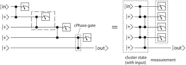
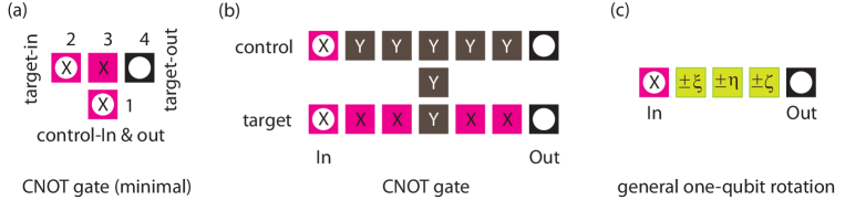
Can we build a general one qubit unitary by concatenating the circuit of Eq. (11)? This is indeed possible. As shown in Fig. 3, we concatenate the circuit Eq. (11) four times, whereby a fifth qubit is transformed into the state $|\psi^{(5)}\rangle=U|{\rm in}\rangle$, with the unitary gate $U$ given by [40]

$$U(\{\phi,s\})=\big{(}He^{i\phi_{4}Z/2}Z^{s_{4}}\big{)}\big{(}He^{i\phi_{3}Z/2}Z^{s_{3}}\big{)}\big{(}He^{i\phi_{2}Z/2}Z^{s_{2}}\big{)}\big{(}He^{i\phi_{1}Z/2}Z^{s_{1}}\big{)}.$$ (16)

We set $\phi_{1}=0$. Then, by reordering operations in the same way as in Eq. (15), can rewrite the resulting unitary as

$$U(\{\phi_{2},\phi_{3},\phi_{4},s\})=Z^{s_{1}+s_{3}}X^{s_{2}+s_{4}}\exp\left(i(-1)^{s_{1}+s_{3}}\frac{\varphi_{4}}{2}X\right)\exp\left(i(-1)^{s_{2}}\frac{\varphi_{3}}{2}Z\right)\exp\left(i(-1)^{s_{1}}\frac{\varphi_{2}}{2}X\right).$$ (17)

Therein, we have used the identities $HZ=XH$ and $XZ=-ZX$, and dropped an overall phase factor. Thus, up to byproduct operator $U_{\Sigma}\equiv Z^{s_{1}+s_{3}}X^{s_{2}+s_{4}}$, a general one-qubit rotation

$$U_{\rm rot}=\exp\left(-i\frac{\zeta}{2}X_{i}\right)\exp\left(-i\frac{\eta}{2}Z_{i}\right)\exp\left(-i\frac{\xi}{2}X_{i}\right),$$ (18)

with Euler angles $\zeta$, $\eta$, $\xi$ can be realized by the choosing the measurement angles

$$\begin{array}[]{rcl}\varphi_{1}&=&0,\\ \varphi_{2}&=&-(-1)^{s_{1}}\xi,\\ \varphi_{3}&=&-(-1)^{s_{2}}\eta,\\ \varphi_{4}&=&-(-1)^{s_{1}+s_{3}}\zeta.\end{array}$$ (19)

We find that measurement angles, and thus measurement bases, depend on measurement outcomes of other qubits. This is the origin of temporal order in measurement-based quantum computation.

The reader will have noted that we could have accomplished the same task of implementing a general one-qubit unitary by concatenating the circuit Eq. (11) only three times rather than four, and not setting the first measurement angle to zero. However, then the Hadamard gates in the counterpart of Eq. (17) would not cancel. We would still obtain a general one-qubit unitary, albeit not in Euler normal form.

3.3 MBQC is universal

To prove universality of MBQC, we need to show that (i) A universal set of gates can be simulated, (ii) Gate simulations compose in the same way as the gates themselves, and (iii) Cluster qubits not required in a particular computation can be removed.

3.3.1 Simulating a universal set of gates

We need to be able to simulate a so-called universal set of gates. Such gate sets have the property that any unitary transformation on an $n$-qubit Hilbert space, for any $n\in\mathbb{N}$, can be arbitrarily closely approximated by gates from the set.

A standard universal gate set consists of all one-qubit rotations for each qubit and the controlled Not (CNOT) gate on any pair of qubits [39]. These gates are defined as

$$\begin{array}[]{rcl}U_{i}&=&\exp\left(-i\frac{\zeta}{2}X_{i}\right)\exp\left(-i\frac{\eta}{2}Z_{i}\right)\exp\left(-i\frac{\xi}{2}X_{i}\right),\\ \mbox{CNOT}_{c,t}&=&|0\rangle_{c}\langle 0|\otimes I_{t}+|1\rangle_{c}\langle 1|\otimes X_{t}.\end{array}$$ (20)

Therein, the subscripts $i$, $c$ (control), $t$ (target) are qubit labels, and $\zeta$, $\eta$ and $\xi$ are the Euler angles specifying the one-qubit rotation $U\in SU(2)$. $X$, $Z$ are Pauli operators ($X\equiv\sigma_{x},\,Y\equiv\sigma_{y},\,Z\equiv\sigma_{z}$). Note that in the above gate set, only the CNOT gate has the power to entangle. It is equivalent, up to local unitaries, to the cPhase gate introduced in Eq. (2).

An MBQC can be split up into MBQC gate simulations. Each gate simulation is like a LEGO piece, with example patterns shown in Fig. 4, which were explained in the previous section. Be ${\cal{C}}$ a set of qubits, with $I\subset{\cal{C}}$ a set of input qubits, $O\subset{\cal{C}}$ a set of output qubits, and ${\cal{C}}\backslash O$ the set of qubits which are in ${\cal C}$ but not in $O$. Then, an MBQC gate simulation on ${\cal{C}}$ is the following

Procedure MBQC-GS.

1. Create a cluster state with input $|\text{in}\rangle$, $|\phi(\text{in})\rangle=\left(\prod_{(a,b)\in E}\mbox{cPhase}_{a,b}\right)|\text{in}\rangle_{I}\bigotimes_{c\in{\cal{C}}\backslash I}|+\rangle_{c}$.

2. Measure all qubits $a\in{\cal{C}}\backslash O$, keep the state $|\text{out}\rangle_{O}$ of the unmeasured qubits in $O$.

The transformation $|\text{in}\rangle\longrightarrow|\text{out}\rangle$ is unitary if suitable local measurement bases and sets $I,O$ are chosen. Specifically, cluster qubits which are not measured in the eigenbasis of $Z$ are measured in a basis in the equator of the Bloch sphere. The measured observable on such a qubit $a\in{\cal{L}}_{2}$ is

$$O_{a}(\varphi_{a})=\cos\varphi_{a}\,X_{a}+\sin\varphi_{a}\,Y_{a},\;\;-\frac{\pi}{2}<\varphi_{a}\leq\frac{\pi}{2}.$$ (21)

The angle $\varphi_{a}$ specifying the measured observable $O_{a}$ is

called the ‘measurement angle’ for qubit $a$.

Figure 4: Measurement patterns for a universal set of gates. (a,b) CNOT, (c) general one-qubit rotation. The CNOT gate in (a) has the control input and output located on the same cluster qubit. The extended CNOT in (b) has separate locations for input and output qubits, for both control and target.

One-qubit rotations.

We return to the procedure of performing a general one-qubit unitary by iterating the circuit Eq. (11) four times, c.f. Section 3.2. By moving cPhase gates backwards in time past local measurements they commute with, we can rewrite this circuit as preparation of a cluster state with one qubit of input, followed by local measurements of four cluster qubits including the input. The necessary re-ordering is displayed in Fig. 3. The circuit on the r.h.s. of Fig. 3 precisely matches the procedure MQC-GS for gate simulations, which completes the construction.

CNOT-gate.

A cluster state of four qubits allows for a simulation of a controlled-NOT gate. Consider the graph shown in Fig. 4a. Let qubits 1 and 2 be in the states $(a|0\rangle_{1}+b|1\rangle_{1})$ and $(c|0\rangle_{2}+d|1\rangle_{2})$, respectively, and qubits 3 and 4 in the state $|+\rangle$. Now, a control-phase gate is applied between pairs $(1,3)$, $(2,3)$, and $(3,4)$. The joint state becomes

$$|\psi\rangle_{1234} = {\rm cPhase}_{43}{\rm cPhase}_{13}{\rm cPhase}_{23}\Big{[}(a|0\rangle_{1}+b|1\rangle_{1})(c|0\rangle_{2}+d|1\rangle_{2})|+\rangle_{3}|+\rangle_{4}\Big{]},$$

$$= \Big{[}a|0\rangle_{1}(c|0\rangle_{2}|+\rangle_{3}+d|1\rangle_{2}|-\rangle_{3})+b|1\rangle_{1}(c|0\rangle_{2}|-\rangle_{3}+d|1\rangle_{2}|+\rangle_{3})\Big{]}|0\rangle_{4}$$

$$+\Big{[}a|0\rangle_{1}(c|0\rangle_{2}|-\rangle_{3}+d|1\rangle_{2}|+\rangle_{3})+b|1\rangle_{1}(c|0\rangle_{2}|+\rangle_{3}+d|1\rangle_{2}|-\rangle_{3})\Big{]}|0\rangle_{4},$$

where we have ignored overall normalization and have chosen a specific sequence of applying the commuting cPhase gates. Let us measure qubits 2 and 3 in the basis $|\pm\rangle$ and record the respective eigenvalues by $(-1)^{s_{2}}$ and $(-1)^{s_{3}}$ respectively. Suppose the measurement outcomes are $+1$, $+1$, i.e., $s_{2}=s_{3}=0$, then the post-measurement joint state of qubits 1 and 4 is

$$|\psi^{\prime}\rangle_{14} = {}_{23}\langle++|\cdot|\psi\rangle_{1234}$$

$$= a|0\rangle_{1}(c|0\rangle_{4}+d|1\rangle_{4})+b|1\rangle_{1}(c|1\rangle_{4}+d|0\rangle_{4})$$

$$= {\rm CNOT}_{14}(a|0\rangle_{1}+b|1\rangle_{1})(c|0\rangle_{4}+d|1\rangle_{4}).$$

We see two effects: (i) there is a control-NOT gate applied on initial qubits 1 and 2 and then (ii) the information on qubit 2 has been transferred to qubit 4. Analyzing the three other cases $(s_{2},s_{3})\in\{(0,1),(1,0),(1,1)\}$, we conclude that the output state $|\psi_{\rm out}\rangle$ on qubits 1 and 4 is related to the input state $|\psi_{\rm in}\rangle$ on qubits 1 and 2 via the transformation

$$|\psi_{\rm out}\rangle={\rm CNOT}\,X_{t}^{s_{3}}Z_{t}^{s_{2}}|\psi_{\rm in}\rangle=Z_{c}^{s_{2}}X_{t}^{s_{3}}Z_{t}^{s_{2}}{\rm CNOT}|\psi_{\rm in}\rangle,$$ (22)

with qubit 1 acting as control qubit. We remark that qubits 2 and 3 are always measured in the $X$-eigenbasis, independent of all measurement outcomes on the cluster qubits. Therefore, the measurements on those qubits can be performed first, and the MBQC simulation of CNOT gates entirely drops out of the temporal order of measurements. The same holds for all gate simulations requiring only $X$ and $Y$-measurements, such as the simulations of Hadamard gates and rotations $\exp(i\pi/4\,Z)$.

The minimal configuration Fig. 4a for a CNOT realized on a four qubit cluster has the property that control input and output are located on the same cluster qubit. This may be a disadvantage for the composition of gate simulations. The minimal configuration can be expanded such that the locations for target input, control input, target output and control output are all separate; See Fig. 4b.

Composition of gate simulations.

It remains to be shown that MBQC gate simulations compose like the simulated gates themselves. This proceeds by a reordering-of-commuting-operations argument [23, 24],[40]; also see Fig. 3 for an example. Finally, note that the composition of gate simulations allow for a variable input that the standard cluster state does not provide. Starting with a cluster state amounts to fixing the initial state of the simulated quantum register in the state $\otimes_{i}|+\rangle_{i}$, which is the fiducial state appearing in DiVincenzo’s second criterion.

Removing redundant cluster qubits.

If a two-dimensional cluster state is used to perform measurement-based quantum computation by simulating the universal gates as pattern of measurement (see Fig. 4), these patterns may not cover all of the qubits on the two-dimensional grid. Cluster qubits such as those that are neither covered by the gate-simulation measurement patterns are not needed in a particular computation can be removed by measuring them in the $Z$-eigenbasis. Then, the remaining qubits are still in a cluster state, with the $Z$-measured qubits removed from the cluster. This follows directly from the creation procedure Eq. (2) for cluster states, and the identities $|0\rangle_{a}\langle 0|\,\mbox{cPhase}_{a,b}=|0\rangle_{a}\langle 0|\otimes I_{b}$, $|1\rangle_{a}\langle 1|\,\mbox{cPhase}_{a,b}=|1\rangle_{a}\langle 1|\otimes Z_{b}$. Hence, if one measures any qubit on a cluster state in the $Z$-basis, obtaining an outcome $0$, the remaining qubits are exactly in a cluster state (as they are acted on by identity operators), with the measured qubit removed from the cluster. If the measurement outcome is $1$, then the resulting state is equivalent to cluster state, up to local unitaries $Z$ on qubits neighboring the measured one. This completes the proof that the MBQC can efficiently simulate the circuit model of quantum computation.

4 Ground states as computational resources

For $n$-qubit quantum states distributed according to the uniform Haar measure, it has been shown that only a tiny fraction $<\exp(-n^{2})$ of states can possibly be universal resources for MBQC [36, 37]. We will review this result for a different reason in Section 5.2. Universal resource states thus seem very rare, but is the uniform Haar measure the right criterion to apply? Do resource states for measurement-based quantum computation occur naturally in physical systems, say as ground states of Hamiltonians with two-body interactions?

Let us first drop the requirement of computational universality, and ask the more modest question of whether ground states of suitably simple Hamiltonians can be used as resource states for MBQC at all. This will lead us to one-dimensional spin systems, and provide hints for identifying a computationally universal ground state in a second step.

4.1 Spin chains

In 1983, Haldane argued that the spin-$S$ Heisenberg antiferromagnetic chain has different behaviors depending on $S$ is integer or half-integer [43]. In particular, he predicted that when $S$ is an integer, the spin chain has a unique disordered ground state with a finite spectral gap. This picture was supported by a construction that Affleck, Kennedy, Lieb and Tasaki (AKLT) proposed in a spin-1 valence-bond model [44, 45]. The spin-1 AKLT model and the antiferromagnetic chain are later found to be in the so-called Haldane phase of the following bilinear-biquadratic model,

$$H=\sum_{i}\left[\cos\theta(\vec{S}_{i}\cdot\vec{S}_{i+1})+\sin\theta(\vec{S}_{i}\cdot\vec{S}_{i+1})^{2}\right],$$ (23)

for $\theta\in(-\pi/4,\pi/4)$, where $\vec{S}$ denotes the spin operators for the spin-1 particle. The one-dimensional Affleck-Kennedy-Lieb-Tasaki (AKLT) state is a special point in the Haldane phase with $\tan\theta=1/3$. For periodic boundary conditions, the ground state in the Haldane phase is unique. For a linear chain, it is four-fold (near) degenerate, with the splitting in the degeneracy being exponentially small in the length of the chain. There, both edges carry an effective spin-1/2 particle. The resulting edge states turn out to be very important for our description of MBQC using ground states in the Haldane phase.

If the chain is terminated by a spin-1/2 particle at one end with the additional Hamiltonian term $\sim\vec{S}\cdot\vec{s}$, then the degeneracy is reduced to 2, resulting from an effective spin-1/2 at the other end. The system thus carries total spin-1/2, i.e., $S_{\rm tot}=1/2$ with the effective two levels being $|G_{0}\rangle\equiv\Big{|}S_{\rm tot}=1/2,S_{\rm tot}^{z}=1/2\Big{\rangle}$ and $|G_{0}\rangle\equiv\Big{|}S_{\rm tot}=1/2,S_{\rm tot}^{z}=-1/2\Big{\rangle}$. The degenerate ground space can be used to encode the information of a qubit: $|\Psi\rangle=a_{0}|G_{0}\rangle+a_{1}|G_{1}\rangle$.

As a first result demonstrating the usefulness of Haldane ground states for MBQC, it has been shown that the AKLT state allows to simulate arbitrary single-qubit unitary gates by single-spin measurements [46, 47, 48]; also see [49]. This is not sufficient for universal quantum computation, but it provides a first connection between MBQC and spin systems which have been studied in condensed matter physics for completely different reasons.

Furthermore, if we slightly extend our computational model to comprise of two primitives, namely (i) Measurement of individual spins (as before) and (ii) adiabatic turn-off of individual spin-spin couplings in the Hamiltonian Eq. (23), then a more general result can be obtained: The usefulness of the ground state of Eq. (23) as computational resource extends to the entire Haldane phase surrounding the AKLT point [50]! This is interesting in several ways. For example, away from the AKLT point, the ground state of the spin chain is not explicitly known. Quantum computation by local measurement on those states works perfectly nonetheless. Furthermore, whereas quantum computation is usually considered ‘high maintenance’, i.e. any imperfect control of the system Hamiltonian quickly leads the computation off track, here we observe a feature of robustness: $\theta$ may vary largely without affecting the functioning of the computational scheme. These features are consequences of a symmetry-protected topological order [51, 52] which characterizes the Haldane phase.

We now describe quantum computation by local measurements in the Haldane phase, following the original discussion by Miyake [50]. Let us denote by $|G_{0}(j)\rangle$ and $|G_{1}(j)\rangle$ the two degenerate ground states for a system of spins from $j$ to $N$, and by $|\Psi(j)\rangle$ a qubit state encoded in the ground state space, $|\Psi(j)\rangle=a_{0}|G_{0}(j)\rangle+a_{1}|G_{1}(j)\rangle$. Suppose we start with a chain of $N$ spins in the state $|\Psi(j=1)\rangle$, for known $a_{0}$, $a_{1}$. We can ask how this state is transformed when we turn off adiabatically the coupling between the first and the second spin. The initial value of the total spin is 1/2. After turning off the coupling, the subsystem of spins $(2,..,N)$ by itself is effectively a spin-1/2, residing in the ground space spanned by $|G_{0}(j=2)\rangle$ and $|G_{1}(j=2)\rangle$. Composing it with the spin 1 at site 1, by angular moment addition $1/2\otimes 1=1/2\oplus 3/2$, the final Hamiltonian has ground states with spin 1/2 and 3/2. However, while the coupling is being turned off, rotational symmetry is maintained and the total spin conserved. The final state is thus confined to the spin 1/2 sector. Using the Clebsch-Gordan decomposition, one finds

$$|\Psi(1)\rangle\rightarrow|\Psi^{\prime}(1)\rangle=\sqrt{\frac{2}{3}}\left[\big{(}\frac{a_{0}}{\sqrt{2}}|0\rangle_{1}+a_{1}|-1\rangle_{1}\big{)}\otimes|G_{0}(2)\rangle-\big{(}a_{0}|+1\rangle_{1}+\frac{a_{1}}{\sqrt{2}}|0\rangle_{1}\big{)}\otimes|G_{1}(2)\rangle\right].$$ (24)

After the adiabatic turning-off of the coupling, one can measure the first spin in any orthonormal basis spanned by $|\pm 1\rangle$ and $|0\rangle$. For example, we consider the basis $\big{\{}|x\rangle\equiv(|-1\rangle-|1\rangle)/\sqrt{2},|y\rangle\equiv(|-1\rangle+|1\rangle)/\sqrt{2},|z\rangle\equiv|0\rangle\big{\}}$. After measuring spin 1 in the state $|\beta\rangle$, the post-measurement state of the spins $(2,..,N)$ is ${}_{1}\langle\beta|\cdot|\Psi^{\prime}(1)\rangle$. This state behaves as if a quantum gate had acted on the system $(2,..,N)$ with the initial state $|\Psi(j=2)\rangle=a_{0}|G_{0}(2)\rangle+a_{1}|G_{1}(2)\rangle$. Depending on the measurement outcome ($|\beta=|x\rangle,|y\rangle,|z\rangle$, respectively), the resulting state is

$$X|\Psi(2)\rangle,\ XZ|\Psi(2)\rangle,\ Z|\Psi(2)\rangle.$$ (25)

Therein, $X$ and $Z$ are the effective Pauli X and Z operators, with $X=|G_{0}\rangle\langle G_{1}|+|G_{1}\rangle\langle G_{0}|$ and $Z=|G_{0}\rangle\langle G_{0}|-|G_{1}\rangle\langle G_{1}|$. One may proceed to adiabatically turn off the subsequent couplings one by one and measure the decoupled qubits in the basis $\{|x\rangle,|y\rangle,|z\rangle\}$. Up to the above Pauli rotations, this results in a quantum wire in which a logical qubit is propagated forward along the spin chain.

This process is easily generalized to induce an arbitrary rotation on the effective qubit state. For example, the basis

$${\cal{B}}(\alpha)=\Big{\{}\frac{(1\pm e^{-i\alpha})}{2}|x\rangle_{j}+\frac{(1\mp e^{-i\alpha})}{2}|y\rangle_{j},|z\rangle_{j}\Big{\}}$$ (26)

gives rise to a rotation about $z$-axis $R^{z}(\alpha)=|G_{0}\rangle\langle G_{0}|+e^{i\alpha}|G_{1}\rangle\langle G_{1}|$, up to possible Pauli corrections. Measurement in another basis can induce rotation about other axes, such as $x$-axis. Therefore, arbitrary single-qubit unitary evolution can be simulated in a chain residing in the Haldane phase.

Let us briefly comment on the role of symmetries which protect the Haldane phase [51, 52] and computation on its edge states. It has been shown that the Haldane phase is protected even in the presence of perturbations, as long as they possess certain symmetries such as time reversal [52], $S_{k}^{x,y,z}\longrightarrow-S_{k}^{x,y,z}$. Now, the Hamiltonian Eq. (23), even with individual couplings turned off one by one, has this symmetry. The measured observables with eigenbases Eq. (26) possess it as well, such that the Haldane phase remains protected throughout the course of computation.

It needs to be pointed out that in the above construction, the adiabatic switching-off of couplings is not merely a means to extract individual spins from a ‘ground-state memory’. Away from the AKLT point, turning off a coupling does real work for the computational scheme by modifying the correlation with the edge states. Thus, the question arises of whether the same computational power can be obtained without the adiabatic part. I.e., are ground states of spin chains in the Haldane phase resources for 1-qubit MBQC?

The answer is again affirmative. As shown by Bartlett and collaborators [53], local measurements on a Haldane ground state can be used to mimic a renormalization group transformation. The resulting state is again in the Haldane phase, with the length of the spin chain cut by a factor of three. The AKLT state is a fixed point of this transformation to which the whole Haldane phase is attracted. Thus, to simulate a one-qubit universal MBQC on a ground state in the Haldane phase, a first set of local measurements is used to bring the initial state as close as needed to an AKLT state, and the remaining measurements simulate the unitary gate.

4.2 Universal MBQC with AKLT states in two dimensions

In the previous section we have identified an entire phase of ground states which can serve as resources for restricted measurement-based quantum computations. Beautiful and unexpected connections between measurement-based quantum computation and condensed matter physics have been found as a bonus. But a central question is so far unanswered: Are there ground states of two-body Hamiltonians which are universal resources for MBQC?

The answer again is ‘yes’. This was first established for spin 5/2 particles on a honeycomb lattice [54], with a suitably tailored Hamiltonian. This result is important, because it had previously been proven that cluster states, the standard resource for universal MBQC, cannot arise as the ground state of a Hamiltonian with only two-body interactions [55]. They can nonetheless be closely approximated by ground states of such Hamiltonians [56].

What remains to be explored is whether Hamiltonians with universal resources for MBQC as ground states can look simpler, more natural. In this regard, it was first shown that the unique ground state of an AKLT-like Hamiltonian for spins 3/2 on a two-dimensional lattice Hamiltonian yields a universal resource for MBQC [57]. Here, AKLT-like means that within the two-dimensional lattice, 1D quasi-chains are coupled via the AKLT Hamiltonian, and the coupling between the chains is of a different type, but still two-body.

Finally, it has been shown by Miyake [58] and by Wei, Affleck and Raussendorf [59] that the AKLT state on the honeycomb lattice is a universal computational resource. To briefly review this result, let us first recall the definition of the AKLT state on a honeycomb lattice.

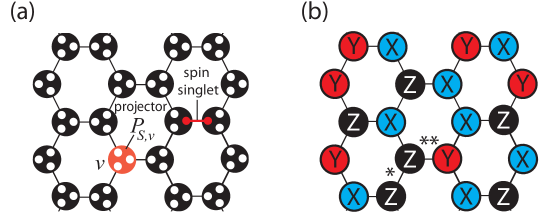
The AKLT state [44] on the honeycomb lattice ${\cal{L}}$ has one spin-3/2 per site of ${\cal{L}}$. The state space of each spin 3/2 can be viewed as the symmetric subspace of three virtual spin-1/2’s, i.e., qubits. In terms of these virtual qubits, the AKLT state on ${\cal{L}}$ is

$$|\Phi_{\rm AKLT}\rangle\equiv\bigotimes_{v\in V({\cal{L}})}P_{S,v}\bigotimes_{e\in E({\cal{L}})}|\phi\rangle_{e},$$ (27)

where $V({\cal L})$ and $E({\cal L})$ to denote the set of vertices and edges of ${\cal L}$, respectively. $P_{S,v}$ is the projection onto the symmetric (equivalently, spin 3/2) subspace at site $v$ of ${\cal{L}}$. For an edge $e=(v,w)$, $|\phi\rangle_{e}$ denotes a singlet state, with one spin 1/2 at vertex $v$ and the other at $w$.

The first step in the process of MBQC with the AKLT state is to apply a suitable generalized measurement [39], also called positive-operator-value measure (POVM), locally on every site $v$ on the honeycomb lattice ${\cal{L}}$; See Fig. 5. Specifically, the POVM consists of three rank-two elements

$${F}_{v,z} = \sqrt{\frac{2}{3}}\left(\left|\frac{3}{2},\frac{3}{2},z\right\rangle\left\langle\frac{3}{2},\frac{3}{2},z\right|+\left|\frac{3}{2},-\frac{3}{2},z\right\rangle\left\langle\frac{3}{2},-\frac{3}{2},z\right|\right)=\frac{1}{\sqrt{6}}\left(S_{z}^{2}-\frac{1}{4}\right),$$ (28a)

$${F}_{v,x} = \sqrt{\frac{2}{3}}\left(\left|\frac{3}{2},\frac{3}{2},x\right\rangle\left\langle\frac{3}{2},\frac{3}{2},x\right|+\left|\frac{3}{2},-\frac{3}{2},x\right\rangle\left\langle\frac{3}{2},-\frac{3}{2},x\right|\right)=\frac{1}{\sqrt{6}}\left(S_{x}^{2}-\frac{1}{4}\right),$$ (28b)

$${F}_{v,y} = \sqrt{\frac{2}{3}}\left(\left|\frac{3}{2},\frac{3}{2},y\right\rangle\left\langle\frac{3}{2},\frac{3}{2},y\right|+\left|\frac{3}{2},-\frac{3}{2},y\right\rangle\left\langle\frac{3}{2},-\frac{3}{2},y\right|\right)=\frac{1}{\sqrt{6}}\left(S_{y}^{2}-\frac{1}{4}\right),$$ (28c)

where $\textbf{r}=x,y,z$ in $|s,m_{s},\textbf{r}\rangle$ specifies the quantization axis. The above POVM elements obey the relation $\sum_{\nu\in\{x,y,z\}}F^{\dagger}_{v,\nu}F_{v,\nu}=I_{S,v}$, which is the identity on the spin-3/2 Hilbert space as well as on the symmetric subspace of three qubits, as required. Physically, $F_{v,a_{v}}$ is proportional to a projector onto the two-dimensional subspace within the $S_{a}=\pm 3/2$ space, which is the origin of logical qubits in the present construction. The outcomes $x$, $y$ or $z$ of the POVM at the individual sites of ${\cal{L}}$ are random, but short-range correlated. After the results of the POVM at all sites, the post-POVM state becomes $\bigotimes_{v\in V({\cal{L}})}F_{v,a_{v}}\,|\Phi_{AKLT}\rangle$, with $a_{v}=x,y,z$ denoting the POVM outcome at site $v$.

Figure 5: AKLT states. (a) Spin singlets of two virtual spins 1/2 are located on the edges of the honeycomb lattice. $P_{S,v}$ is a projection at each lattice site $v$ onto the symmetric subspace. (b) The first step in MBQC with AKLT states is a local POVM at each lattice site, with three possible outcomes $x$, $y$, $z$. Edges with the same POVM outcome at the end points (*) are treated differently from edges where the POVM outcomes differ (**).

After using the same initial POVM, the two arguments proceed differently. In [58] a mapping to quantum circuits is pursued, whereas in [59] the AKLT state is mapped to a two-dimensional cluster state which is already known to be universal. Let us very briefly summarize the two arguments.

In [58], it is noted that whenever the POVM outcomes on two neighboring sites differ, then the link in between can be used to implement, along the remaining two orthogonal links, either an elementary computational wire or an entangling gate between two wires. Such links are sufficiently frequent to form a giant connected component [60], from which a ‘backbone’ is chiseled out by further local measurements. The backbone is a net composed of computational wires and bridges between them, similar to the one displayed in Fig. 1a.

The links between neighboring sites with the same POVM outcome cannot be used for entangling gates between wires in the backbone, and represent a (manageable) complication. A connected set of such links ranging from one wire to another compromises those wires, and therefore has to be avoided. Fortunately, identical POVM outcomes on the opposite ends of a link occur only with a probability of approximately 1/3, which is sufficiently infrequent for connected sets of such links to remain microscopic. They can then be dealt with by choosing a sufficiently large-meshed backbone, on which a general quantum circuit may be implemented.

In [59], proof of computational universality proceeds by reduction to a 2D cluster state, via an intermediate step. Namely, it is first shown that applying the local POVMs to the AKLT state results in a graph state. The corresponding graph depends on the random POVM outcomes but is always planar. It is obtained from the graph representing the honeycomb lattice ${\cal{L}}$ using the following rules: (i) If the POVM outcomes on two neighboring vertices agree, the edge in between is contracted, and (ii) in the resulting multigraph, edges of even multiplicity are deleted and edges of odd multiplicity are replaced by standard edges.

Then, typical graphs resulting from this procedure are shown by numerical simulation to reside in the supercritical phase of percolation, i.e., they have traversing paths. Such graph states can then be used to implement universal quantum computation by local measurements, which is demonstrated by reduction to 2D cluster states.

5 The role of entanglement

Hardwired into the very foundations of quantum information science is the assumption that local quantum operations and classical communication (LOCC) are easily accomplished whereas non-local operations, i.e., quantum-mechanical interactions between different parts of a quantum system, are difficult. Consequently, a fundamental distinction is made between these two classes of operations. From this perspective, entanglement [61, 62] is a quintessential property of quantum systems. It measures the degree to which quantum states require non-local operation for their creation or to which they can enable non-local operation. It is also a key resource for many protocols of quantum information processing, such as teleportation, quantum cryptography, and quantum error-correction. The defining property of entanglement monotones [63], which measure the ‘amount’ of entanglement contained in quantum states, is that they do not increase under LOCC.

Since MBQC is driven entirely by operations in the LOCC class, entanglement decreases as the computation proceeds. This provides our intuition that entanglement is a key resource for MBQC. A closer examination shows that, for quantum computation with pure resource states, significant entanglement is indeed necessary to achieve a quantum speedup, but more is not necessarily better.

5.1 Entanglement and quantum speedup

In this section, we demonstrate that any MBQC with a pure state that only contains a small amount of entanglement can be efficiently classically simulated, preventing a significant speedup (See [64] for an analogous result in the circuit model). To do so, we must first overcome an obstacle.

Consider cluster state $|\phi_{\cal{C}}\rangle$ on a one-dimensional cluster ${\cal{C}}$. As illustrated by the example of simulating a general one-qubit rotation, MBQC on one-dimensional cluster states maps to the circuit model with a single qubit. It can thus be efficiently simulated classically. And yet, $|\phi_{\cal{C}}\rangle$ is highly entangled. For suitable bi-partitions ${\cal{C}}=A\cup B$ (e.g. odd vs. even-numbered qubits), the von-Neumann entropy $E_{A:B}(|\phi\rangle):=S(\rho_{A})=-\mbox{Tr}(\rho_{A}\log\rho_{A})=S(\rho_{B})$, which is a valid entanglement measure for pure states [65], takes the large value of $E_{A:B}(|\phi_{\cal{C}}\rangle)=\lfloor|{\cal{C}}|/2\rfloor$. To rescue the asserted connection between entanglement and speedup, we need to look for a different entanglement measure.

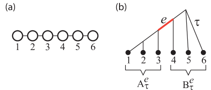
To this end, for general pure states $|\psi\rangle$ on a set $V$ of qubits, consider a subcubic tree $T$ (a tree graph with vertices of degrees between 1 and 3) whose leaves (vertices of degree 1) are associated with the qubits in $V$. For any edge $e$ of $T$, $T\backslash e$ consists of two components, inducing a bi-partition of $V$ into two sets $A_{T}^{e}$ and $B_{T}^{e}$. It can be shown [66, 67] that the quantity

$$E_{\rm wd}(|\psi\rangle)\equiv\min_{T}\max_{e\in T}E_{A_{T}^{e},B_{T}^{e}}(|\psi\rangle).$$ (29)

is an entanglement monotone. It is called ‘entanglement width’.

Returning to our above example of the one-dimensional cluster state $|\phi_{\cal{C}}\rangle$, it turns out that $E_{\rm wd}(|\phi_{\cal{C}}\rangle)=1$. To see this, note that for the tree $\tau$ displayed in Fig. 6 b, the von Neumann entropy with respect to the bi-partition $A_{\tau}^{e}:B_{\tau}^{e}$ is $E_{A_{\tau}^{e},B_{\tau}^{e}}(|\phi_{\cal{C}}\rangle)=1$, for any $e\in E(\tau)$. Thus, the entanglement width does at least remove the above counterexample towards establishing a connection between entanglement and hardness of classical simulation in MBQC. But is it of more general use? Can this entanglement measure, at least for broad classes of interest, be efficiently calculated?

These questions both have affirmative answers. First, calculating the entanglement width is in general hard, due to minimization over all subcubic trees. However, if the state in question is a graph state, then a close upper bound can be obtained efficiently [68], using graph theoretic techniques [69]. Furthermore, the following general result [68] establishes entanglement width as the critical complexity parameter for the classical simulation of MBQC on graph states,

Theorem 1 (van den Nest et al.).

Let $|G\rangle$ be a graph state on $n$ qubits. Then, MBQC on $|G\rangle$ can be classically simulated in $\mbox{poly}(n,2^{E_{\rm wd}(|G\rangle)})$ time.

A similar theorem can be established for general $n$-qubit quantum states instead of graph states only, but it requires extra conditions relating to the efficient computability of the entanglement width [68].

Theorem 1 shows that a substantial amount of entanglement, as measured by the entanglement width, is necessary for a quantum speedup in MBQC with graph states. However, it is not sufficient. MBQC with so-called surface code states [70] on a $k\times k$ lattice, which are local unitary equivalent to graph states, can be efficiently simulated classically in $\mbox{poly}(k)$ time, but their entanglement width is linear in $k$ [71].

A related yet separate question is whether substantial entanglement is required for universality of MBQC. If we consider quantum computation as a universal state preparator, so-called $CQ$-universality, then the answer is affirmative. A family of resource states can only be $CQ$-universal if the entanglement in the belonging states is unbounded [66, 67]. In the preceding discussion of the relation between entanglement and speedup in MBQC, we assumed classical input and output (all qubits were required to be measured), so-called $CC$-universality.

A $CQ$-universal quantum computer presumably has more power than a $CC$-universal quantum computer. It was thus conjectured that $CC$-universal resource states exist which cannot be LOCC-converted to any $CQ$-universal state. Some examples for $CC$-universal states were proposed by Gross and Eisert in the new framework of measurement-based quantum computation with Projected-Entangled-Pair-States (PEPS) [46, 47, 72]. However, it was shown later by Cai et al. [73] that these $CC$-universal states can be locally converted to cluster states, which are $CQ$-universal. Whether or not the notions of $CC$ and $CQ$-universality are equivalent remains an open question.

Figure 6: (a) Linear cluster state C6. (b) Bipartitions induced by a sub-cubic tree, and optimal tree $\tau$.

In the next section, we present a different facet of the relation between entanglement and MBQC which provides a counterpoint to the result just discussed.

5.2 Too entangled to be useful

It came as a surprise when Gross, Flammia and Eisert [36], and independently, Bremner, Mora and Winter [37], showed that if a quantum state is too entangled then it becomes useless for MBQC. They measured the entanglement content in terms of the geometric entanglement (GE) [74]. In [36], it is shown that if an $n$-qubit state $|\Psi_{n}\rangle$ is the resource state for a measurement-based quantum computation that succeeds with high probability, and furthermore $E_{G}(|\Psi_{n}\rangle)>n-\delta$, where $\delta$ is a small constant, then this quantum computation can be efficiently classically simulated. No quantum speedup is provided, and $|\Psi_{n}\rangle$ is thus not useful as a resource state.

Let us recall the definition of geometric measure of entanglement [74]. It is motivated by the mean-field approximation. The idea is to find, among the set of product states, $\{|\Phi\rangle=|\phi^{[1]}\rangle\otimes|\phi^{[2]}\rangle\otimes\cdots\otimes|\phi^{[n]}\rangle\}$, the one closest to $|\psi\rangle$. This is achieved by maximizing their overlap, $\Lambda_{\max}({\psi})\equiv\max_{\Phi}|\langle\Phi|\psi\rangle|$. The GE of $|\psi\rangle$ is then defined as [75]

$$E_{G}(\psi)\equiv-\log_{2}\Lambda_{\max}({\psi})^{2}.$$ (30)

The maximum value of $E_{G}$ for an $n$-qubit state is $n$.

Now, to prove the above claim, consider MBQC on a resource state $|\Psi\rangle$ of $n$ qubits which succeeds with high probability, 1/2 say. Furthermore, assume that $|\Psi\rangle$ has close to maximal geometric entanglement, $E_{G}(|\Psi\rangle)>n-\delta$. Then, there are $2^{n}$ possible measurement outcomes, and we are interested in the fraction of good outcomes $G$ which cause the computation to succeed. The probability of each individual outcome is bounded by $|\langle\alpha|\Psi\rangle|^{2}\leq 2^{-E_{G}(\Psi)}<2^{-n+\delta}$. The success probability $\sum_{\alpha\in G}p(|\alpha\rangle)$ is $\geq 1/2$ by assumption, and thus in turn the fraction of good outcomes is $|G|/2^{n}\geq 2^{-\delta-1}$. The above quantum computation can therefore be efficiently simulated by a classical computer selecting the measurement outcome at random. Since the fraction of good outcomes is large, with high probability after a few trials, a good outcome will be selected. Thus, the above MBQC using a (too) entangled resource state does not perform better than a classical computer.

The conclusion that ‘too much entanglement renders a MBQC resource state useless’ may depend on the entanglement measure chosen. How much so, is presently unknown. However, the GE is a lower bound on other entanglement measures [75, 76], such as the relative entropy of entanglement [77] and the logarithmic robustness of entanglement [78]. The above result holds for those measures as well.

6 The role of quantum correlations

We have shown in Section 3 that the computational output in MBQC bitwise consists of correlations among certain measurement outcomes, and that these correlations derive from the quantum correlations Eq. (7) defining the cluster state. Surely, the correlations Eq. (7) uniquely define a highly entangled quantum state. But is there another sense in which these correlations reveal their quantumness? Yes.—They can in general not be described by a local hidden variable model. Anders and Browne [79] have demonstrated a connection, at least in a specific example, between measurement-based quantum computation and Bell’s theorem [80]. The correlations Eq. (7) feature prominently in this correspondence.

Hidden variable models (HVM) were spurred by Einstein, Podolski and Rosen’s famous paper [81] entitled “Can Quantum Mechanics be considered complete?”. With no additional assumptions made, such theories cannot be ruled out as valid descriptions of physical reality. Bohm’s wave mechanics [82] is a prominent example. However, if the hidden-variable model is required to be local, then—as Bell’s theorem [80] shows—it cannot reproduce all predictions of quantum theory.

For our purpose of relating Bell’s theorem to measurement-based quantum computation, we will revisit Mermin’s proof [83] of Bell’s theorem, using the Greenberger-Horne-Zeilinger (GHZ) states [38]. Consider the quantum state $|GHZ\rangle=\big{(}|000\rangle+|111\rangle\big{)}/{\sqrt{2}}$, which is local unitary equivalent to the three-qubit cluster state $|\phi_{3}\rangle$ (10), as $|GHZ\rangle=H_{1}H_{3}|\phi_{3}\rangle$. It is straightforward to check that $|GHZ\rangle$ is the simultaneous eigenstate with eigenvalue +1 of the four Pauli operators

$$X_{1}X_{2}X_{3},\,-X_{1}Y_{2}Y_{3},\,-Y_{1}X_{2}Y_{3},\,-Y_{1}Y_{2}X_{3}.$$ (31)

Now, a local HVM would assign ‘pre-existing values’ $v(X_{1})$, $v(X_{2})$, $v(X_{3})$, $v(Y_{1})$, $v(Y_{2})$, $v(Y_{3})$ to the observables $X_{1}$, $X_{2}$, $X_{3}$, $Y_{1}$, $Y_{2}$, $Y_{3}$ which are merely revealed by measurement. Can those values be consistently assigned such that the predictions of quantum mechanics are reproduced?

Suppose this is the case. Then, $v(X_{1}),v(X_{2}),..,v(Y_{3})\in\{1,-1\}$. Furthermore,

$$\begin{array}[]{rcr}v(X_{1})\,v(X_{2})\,v(X_{3})&=&1,\\ v(X_{1})\,v(Y_{2})\,v(Y_{3})&=&-1,\\ v(Y_{1})\,v(X_{2})\,v(Y_{3})&=&-1,\\ v(Y_{1})\,v(Y_{2})\,v(X_{3})&=&-1.\end{array}$$ (32)

To see why these constraints need to be enforced, consider the first one as an example. The four Pauli operators $X_{1}$, $X_{2}$, $X_{3}$ and $X_{1}X_{2}X_{3}$ obey the identity $X_{1}\cdot X_{2}\cdot X_{3}=X_{1}X_{2}X_{3}$. Furthermore, they mutually commute and hence can be simultaneously diagonalized. The above identity therefore also holds for their simultaneous eigenvalues, which, according to quantum mechanics, are the possible simultaneous measurement outcomes. Since the HVM is required to reproduce the predictions of quantum mechanics, the same relation must hold for $v(X_{1})$, $v(X_{2})$, $v(X_{3})$ and $v(X_{1}X_{2}X_{3})$. Finally, $v(X_{1}X_{2}X_{3})=1$ by Eq. (31).

But Eq. (32) cannot be satisfied! Multiplying all four equations in (32) we obtain

$$v(X_{1})^{2}\,v(Y_{1})^{2}\,v(X_{2})^{2}\,v(Y_{2})^{2}\,v(X_{3})^{2}\,v(Y_{3})^{2}\,=-1,$$

Since $v(X_{1})^{2}=v(X_{2})^{2}=v(Y_{3})^{2}=1$, this is a contradiction. Hence, no consistent assignment of pre-existing values $v(X_{1}),\,..\,,v(Y_{3})$ exists. The correlations Eq. (31) of the GHZ state cannot be reproduced by a local HVM, and are genuinely quantum mechanical.

As it turns out, the very same correlations power a simple yet illuminating example of MBQC [79]. Consider the task of carrying out a single OR-gate via MBQC, using a GHZ-state as quantum resource and a classical control computer for the pre-processing of measurement bases and post-processing of measurement outcomes. This classical processing has an important constraint, namely that—as usual in MBQC—it can only involve addition mod 2. This kind of computation by itself is very limited.

The computation proceeds as follows. Denote the two input bits to the computation by $a$ and $b$, and the output bit by $o$ of the desired OR gate, $o=a\vee b$. The observable measured on qubit $i$ is $X_{i}$ if $q_{i}=0$, and $Y_{i}$ if $q_{i}=1$. The measurement bases are related to the input $a,b$ via

$$q_{1}=a,\,q_{2}=b,\,q_{3}=a+b\mod 2.$$

The output bit $o$ is related to the measurement outcomes $s_{i}\in\{0,1\}$ of the qubits $i$ via the computation by the classical computer which can only performs AND gates (i.e., binary addition),

$$o=s_{1}+s_{2}+s_{3}\mod 2.$$

Note that the relations specifying the classical pre and post-processing are all linear mod 2, as required.

We now discuss the functioning of the MBQC-OR computer input by input. For example, if $a=b=0$ then the measured observables are $X_{1}$, $X_{2}$ and $X_{3}$. Since $X_{1}X_{2}X_{3}|GHZ\rangle=|GHZ\rangle$ by Eq. (31), $s_{1}+s_{2}+s_{3}\mod 2=0$ for this input. Thus, $o=0=0\vee 0$ as required by the logical table.

As a second example, consider $a=0$ and $b=1$. Then, the measured observables are $X_{1}$, $Y_{2}$ and $Y_{3}$. By Eq. (31), $X_{1}Y_{2}Y_{3}|GHZ\rangle=-|GHZ\rangle$, and therefore $o=s_{1}+s_{2}+s_{3}\mod 2=1=0\vee 1$. The remaining two cases of inputs are analogous, and the logical table of the OR-gate, $o=a\vee b$, is established.

To put this result into perspective, it surely does not take a quantum computer to execute an OR-gate. The present example is therefore of no practical relevance. However, it makes a fundamental point. The classical control computer alone, which is only able to perform addition mod 2, has almost no computational power. In contrast, if mod 2-addition is supplemented by the capability of performing OR-gates, the resulting computational device becomes classically universal. Thus, a supply of GHZ states and the ability to measure them locally leads to a vast increase in the computational power.

What is more, the very same quantum correlations upon which Mermin’s proof of Bell’s theorem rests turn out to power the above measurement-based quantum computation. This result [79] hints at a link between MBQC and non-locality of quantum mechanics. How general this connection is remains to be explored.

7 Conclusion

We have given an introduction to the one-way quantum computer, a scheme of universal quantum computation driven by local measurements on an entangled resource state. After a short explanation of how this scheme of computation works, we have described its underlying computational model, and identified universal resources among ground states of relatively simple Hamiltonians—such as the AKLT state on the honeycomb lattice. Further, we have discussed the roles of entanglement and quantum correlations for this computational model. It should be noted that our knowledge in either of these areas is very incomplete, and the research highlights presented here should be understood as base camps for further exploration.

We would like to end with three questions of varying degree of generality that seem particularly close to condensed matter physics: Is there, similar to the one-dimensional case, a Haldane-like phase around the AKLT state on the honeycomb lattice; and if so, does computational universality extend from the AKLT state to all regions of that phase? Can universal resource states be classified? Can a general theory of quantum correlations for measurement-based quantum computation be established?

Acknowledgment. The authors thank Maarten van den Nest, Dan Browne, Akimasa Miyake, Wolfgang Dür, Hans Briegel, Ian Affleck and Dietrich Leibfried for discussions. This work is supported by NSERC, Cifar and the Sloan Foundation.

References

- [1] Shor PW. 1997. SIAM J. Sci. Statist. Comput. 26:1484
- [2] Unruh WG. 1995. Phys. Rev. A 51:992-97
- [3] Shor PW. 1995. Phys. Rev. A 52:R2493-96
- [4] Steane AM. 1996. Proc. R. Soc. A 452:2551-77
- [5] Gottesman D. 1998. Phys. Rev. A 57:127-37
- [6] Aharonov D, Ben-Or M. 1999. arXiv:quant-ph/9906129
- [7] Aliferis P, Gottesman D, Preskill J. 2006. Quant. Inf. Comput. 6:97-165
- [8] Sarma SD, Freedman M, Nayak C. 2006. Physics Today 7:32-38 (2006).
- [9] Nayak C, Simon SH, Stern A, Freedman M, Das Sarma S. 2008. Rev. Mod. Phys. 80:1083-159
- [10] Vandersypen LMK, Steffen M, Breyta G, Yannoni CS, Sherwood MH, Chuang IL. 2001. Nature 414:883-87
- [11] Greiner M, Mandel O, Hänsch TW, Bloch I. 2002 Nature 419:51-54
- [12] Nelson KD, Li X, Weiss DS. 2007. Nature Phys. 3:556-60
- [13] Blatt R, Wineland, D. 2008. Nature 453:1008-15
- [14] Leibfried D, Knill E, Seidelin S, Britton J, Blakestad RB, et al. 2005. Nature 438:639-42
- [15] Häffner H, Hänsel W, Roos CF, Benhelm J, Chek-al-kar D, et al. Nature 438:643-46
- [16] Moehring DL, Maunz P, Olmschenk S, Younge KC, Matsukevich DN, et al. 2007. Nature 449:68-71
- [17] Walther P, Resch KJ, Rudolph T, Schenck E, Weinfurter H, et al. 2005. Nature 434:169-76
- [18] Niskanen AO, Harrabi K, Yoshihara F, Nakamura Y, Lloyd S, et al. 2007. Science 316:723-26
- [19] Harris R, Johnson MW, Lanting T, Berkley AJ, Johansson J, et al. 2010. Phys. Rev. B 82:024511
- [20] Hughes R, Doolen G, Awschalom DA, Chapman M, Clark R, et al. 2004. A Quantum Information and Technology Roadmap, Part I: Quantum Computation in Report of the Quantum Information Science and Technology Experts Panel to ARDA
- [21] Feynman RP. 1948. Rev. Mod. Phys. 20:367-87
- [22] Gottesman D, Chuang IL. 1999. Nature 402:390-93 (1999)
- [23] Raussendorf R, Briegel HJ. 2001. Phys. Rev. Lett. 86:5188-91
- [24] Raussendorf R, Browne DE, Briegel HJ. 2003. Phys. Rev. A 68:022312
- [25] Briegel HJ, Browne DE, Dür W, Raussendorf R, and Van den Nest M. 2009. Nature Phys. 5:19-26
- [26] Briegel HJ, Raussendorf R. 2001. Phys. Rev. Lett. 86:910-13
- [27] Greiner M, Mandel O, Esslinger T, Hänsch TW, Bloch I. 2002. Nature 415:39-44
- [28] Bakr WS, Peng A, Tai ME, Ma R, Simon J, et al. 2010. Science 329:547-50
- [29] Barrett SD, Kok P. 2005. Phys. Rev. A 71:060310(R)
- [30] Duan LM, Raussendorf R. 2005. Phys. Rev. Lett. 95:080503
- [31] Knill E, Laflamme R, Milburn GJ. 2001. Nature 409:46-52
- [32] Nielsen MA. 204. Phys. Rev. Lett. 93:040503
- [33] Browne DE, Rudolph T. 2005. Phys. Rev. Lett. 95:010501
- [34] Yoran N, Reznik B. 2003. Phys. Rev. Lett. 91:037903
- [35] Grover LK. 1996. A fast quantum mechanical Algorithm for database search. In Proc. 28 Annual ACM Symp. on the Theory of Computing:212
- [36] Gross D, Flammia ST, Eisert J. 2009. Phys. Rev. Lett. 102:190501
- [37] Bremner MJ, Mora C, Winter A. 2009. Phys. Rev. Lett. 102:190502
- [38] Greenberger DM, Horne MA, Zeilinger A. 1989. In Bell’s Theorem, Quantum Theory, and Conceptions of the Universe, ed. Kafatos M. 69. Dordrecht: Kluwer
- [39] Nielsen MA, Chuang IL. 2000. Quantum Computation and Quantum Information. Cambridge: Cambridge University Press
- [40] Childs AM, Leung DW, Nielsen MA. 2005. Phys. Rev. A 71:032318
- [41] Raussendorf R, Briegel HJ. 2002. Quant. Inf. Comp. 2:443-86
- [42] Browne DE, Kashefi E, Mhalla M, Perdrix S. 2007. New J. Phys. 9:250
- [43] Haldane FDM. 1983. Phys. Lett. A 93:464-68; Haldane FDM. 1983. Phys. Rev. Lett. 50:1153-56
- [44] Affleck I, Kennedy T, Lieb EH, Tasaki H. 1987. Phys. Rev. Lett. 59:799-802
- [45] Affleck I, Kennedy T, Lieb EH, Tasaki H. 1988. Comm. Math. Phys. 115:477-528
- [46] Gross D, Eisert J. 2007. Phys. Rev. Lett. 98:220503
- [47] Gross D, Eisert J, Schuch N, and Perez-Garcia D. 2007. Phys. Rev. A 76:052315
- [48] Brennen GK, Miyake A. 2008. Phys. Rev. Lett. 101:010502.
- [49] Chen X, Duan R, Ji Z, Zeng B. 2010. Phys. Rev. Lett. 105:020502.
- [50] Miyake A. 2010. Phys. Rev. Lett. 105:040501
- [51] Gu ZC, Wen XG. 2009. Phys. Rev. B 80:155131
- [52] Pollmann F, Turner AM, Berg E, Oshikawa M. 2010. Phys. Rev. B 81:064439
- [53] Bartlett SD, Brennen GK, Miyake A, Renes JM. 2010. Phys. Rev. Lett. 105:110502
- [54] Chen X, Zeng B, Gu ZC, Yoshida B, Chuang IL. 2009. Phys. Rev. Lett. 102:220501
- [55] Nielsen MA. 2006. Rep. Math. Phys. 57:147-61
- [56] Rodolph T, Bartlett SD. 2006. Phys. Rev. A 74:040302(R)
- [57] Cai J, Miyake A, Dür W, Briegel HJ. 2010. Phys. Rev. A 82:052309
- [58] Miyake A. 2010. e-print arXiv:1009.3491
- [59] Wei TC, Affleck I, Raussendorf R. 2011. Phys. Rev. Lett. 106:070501
- [60] Durrett R. 2007. Random Graph Dynamics pp. 27 - 69. Cambridge/New York: Cambridge University Press
- [61] Plenio MB, Virmani S. 2007. Quantum Inf. Comput. 7:1-51
- [62] Horodecki R, Horodecki P, Horodecki M, Horodecki K. 2009. Rev. Mod. Phys. 81:865
- [63] Vidal G. 2000. J. Mod. Opt. 47: 355-76
- [64] Vidal G. 2003. Phys. Rev. Lett. 91:147902.
- [65] Bennett CH, Bernstein HJ, Popescu S, Schumacher. 1996. Phys. Rev. A 53:2046–52
- [66] Van den Nest M, Miyake A, Dür W, Briegel HJ. 2006. Phys. Rev. Lett. 97:150504
- [67] Van den Nest M, Dür W, Miyake A, Briegel HJ. 2007. New J. of Phys. 9:204
- [68] Van den Nest M, Dür W, Vidal, G, Briegel HJ. 2007. Phys. Rev. A. 75: 012337
- [69] Oum SI. 2005. Lect. Notes Comput. Sci. 3787:49-58
- [70] Kitaev A. 2003. Ann. Phys. (N.Y.) 303:2-30
- [71] Bravyi S, Raussendorf R. 2007. Phys. Rev. A 76:022304
- [72] Verstraete F, Cirac JI. 2004. Phys. Rev. A 70:060302(R)
- [73] Cai JM, Dür W, Van den Nest M, Miyake A, Briegel HJ, Phys. Rev. Lett. 103:050503
- [74] We TC, Goldbart PM. 2003. Phys. Rev. A 68:042307
- [75] Wei TC, Ericsson M, Goldbart PM, Munro WJ. 2004. Quantum Inf. Comput. 4: 252-72
- [76] Hayashi M, Markham D, Murao M, Owari M, Virmani S. 2006. Phys. Rev. Lett. 96:040501
- [77] Vedral V, Plenio MB, Rippin MA, Knight PL. 1997. Phys. Rev. Lett. 78: 2275-78
- [78] Vidal G, Tarrach R. 1999. Phys. Rev. A 59:141-55
- [79] Anders J, Browne DE. 2009. Phys. Rev. Lett. 102:50502
- [80] Bell JS. 1964. Physics 1:195
- [81] Einstein A, Podolsky B, Rosen N. 1935. Phys. Rev. 47:777-80
- [82] Bohm D. 1952. Phys. Rev. 85:166-79 and 180-93
- [83] Mermin ND. 1993. Rev. Mod. Phys. 65:803-15