The deep look onto the hard X-ray sky:
The Swift - INTEGRAL X-ray (SIX) survey

Abstract

The super-massive black-holes in the centers of Active Galactic Nuclei (AGN) are surrounded by obscuring matter that can block the nuclear radiation. Depending on the amount of blocked radiation, the flux from the AGN can be too faint to be detected by currently flying hard X-ray (above 15 keV) missions. At these energies only $\sim$1% of the intensity of the Cosmic X-ray Background (CXB) can be resolved into point-like sources that are AGNs. In this work we address the question of the undetected sources contributing to the CXB with a very sensitive and new hard X–ray survey: the SIX survey that is obtained with the new approach of combining the Swift/BAT and INTEGRAL/IBIS X–ray observations. We merge the observations of both missions. This enhances the exposure time and reduces systematic uncertainties. As a result we obtain a new survey over a wide sky area of 6200 deg² that is more sensitive than the surveys of Swift/BAT or INTEGRAL/IBIS alone. Our sample comprises 113 sources: 86 AGNs (Seyfert-like and blazars), 5 galaxies, 2 clusters of galaxies, 3 Galactic sources, 3 previously detected unidentified X-ray sources, and 14 unidentified sources. The scientific outcome from the study of the sample has been properly addressed to study the evolution of AGNs at redshift below 0.4. We do not find any evolution using the 1/V_max method. Our sample of faint sources are suitable targets for the new generation hard X-ray telescopes with focusing techniques.

1 Introduction

In the view of the so-called AGN unified model (Antonucci, 1993; Urry & Padovani, 1995) a super-massive black hole (SMBH) harbored at the center of the AGN powers the nuclear activity. The region where the activity takes place can be observed from different viewing angles. Therefore depending on the orientation of the AGN the observer’s line of sight intercepts different amounts of the optically thick gas–dust structure (torus) that surrounds the SMBH. The nuclear radiation at optical/UV and X-ray wavelengths is efficiently absorbed by the torus. The amount of obscuring matter (N_H column density associated to the torus) can be best inferred by X-ray spectra of the AGNs. X-ray surveys are therefore powerful tools for AGN population studies. The bias of X-ray surveys strongly depends on the column density associated to the sources and the survey sensitivity: the larger the column density and the worse the flux sensitivity, the better the low–absorbed sources are selected. Such selection effect is negligible for unabsorbed sources (exhibiting N_H $<$ 10²² cm^-2) while it affects the absorbed sources (exhibiting N_H $>$ 10²² cm^-2) and it is magnified for sources with column densities N_H $\geq$ 1.5 $\times$ 10²⁴ cm^-2. This latter value corresponds to the inverse of the Thompson cross-section ($\sigma_{T}^{-1}$) and the optical depth unity for Compton scattering. Absorbed sources affected by such high column densities are defined as ”Compton-thick”. This plays an important role in nowadays most sensitive AGN X-ray surveys that are performed by XMM-Newton and Chandra in the energy range $\sim$0.5 - 10 keV (Brandt et al., 2001; Alexander et al., 2003; Cappelluti et al., 2009; Xue et al., 2011). At these energies less than a mere 10% of the nuclear radiation is energetic enough to pierce through the absorbing Compton-thick torus (Gilli et al., 2007). On the other hand the efficiently absorbed optical/UV radiation heats the dust of the obscuring medium, that is expected to waste the absorbed radiation in form of IR emission. Indeed, an IR–excess due to warm dust heated by obscured AGNs has been found (Fadda et al., 2002). Infrared power-law selected samples in Chandra Deep Fields are promising AGN–candidates (Alonso-Herrero et al., 2006; Donley et al., 2007). The drawback of the IR selection is that the majority of the detected sources are not AGNs. Furthermore this approach seems to sample best the sources within redshift 1–3 (Donley et al., 2007). This is the same redshift range in which Chandra and XMM-Newton are preferentially selecting most AGNs in their deep surveys (Brandt & Hasinger, 2005; Hasinger, 2008). Instead the redshift space at z $<$ 0.4 is so far poorly explored despite extensive studies (Markwardt et al., 2005; Beckmann et al., 2006; Sazonov et al., 2007; Ajello et al., 2008b; Tueller et al., 2008; Bird et al., 2010; Cusumano et al., 2010).

The low-redshift (z $<$ 0.4) Universe is best fathomed at hard X–ray energies ($>$ 15 keV). With the advent of the INTEGRAL (Winkler et al., 2003) and the Swift (Gehrels et al., 2004) missions, the selection of local AGNs through their hard X–ray ($>$15 keV) emission has proven to be an extremely powerful technique over the last few years. INTEGRAL and Swift carry coded-mask telescopes on board, namely the Imager on–Board the INTEGRAL Satellite (IBIS: Ubertini et al., 2003) and the Burst Alert Telescope (BAT: Barthelmy et al., 2005) respectively. IBIS has two detector layers. One of which is the INTEGRAL Soft Gamma-Ray Imager (ISGRI: Lebrun et al., 2003). IBIS/ISGRI and BAT have two major advantages: 1) they have a huge field of view, hence allowing to sample an adequate number of AGNs at low-redshift 2) they operate at energies above 15 keV, hence allowing detecting the photons having enough penetrating power to pierce efficiently even through the Compton-thick torus. A further and major advantage in sampling photons above 15 keV from AGNs comes from the emitting source itself. Indeed, a broad continuum bump, so-called ”Compton-reflection bump”, peaking at energies between 20 - 30 keV is produced by reflection of the primary nuclear radiation on the inner side of the obscuring gas (George & Fabian, 1991; Gilli et al., 2007). This spectral component has been found to be dominant in nearby heavily obscured AGNs (Comastri et al., 2007). The Compton-reflection component also plays an important role in reproducing the shape and intensity of the CXB (Rogers & Field, 1991; Gilli et al., 2001; Ueda et al., 2003), that peaks at 30 keV (for most recent measurements see: Ajello et al., 2008b; Moretti, 2009; Türler et al., 2010). Estimates based on observations with PDS (Frontera et al., 1997) on board the BeppoSAX (Boella et al., 1997) satellite predict that Compton-thick AGNs should dominate over unobscured AGNs in the local Universe (Matt et al., 2000). This makes IBIS/ISGRI and BAT well suited instruments for detecting obscured AGNs in the local Universe. IBIS/ISGRI and BAT both represent a major improvement for the imaging of the sky above 15 keV. However coded-mask detectors suffer from heavy systematic effects (errors) preventing them from reaching their theoretical limiting sensitivity (Skinner, 2008). Furthermore by design they block $\sim$50% of the incident photons causing an increase of the statistical noise. These are the reasons that make the detection of extragalactic sources, that are mostly faint, still challenging to undertake. Here we describe an alternative approach which has been developed ad hoc to improve the sensitivity of extragalactic hard X–ray surveys by using IBIS/ISGRI and BAT.

In this paper we show that Swift/BAT and INTEGRAL/IBIS observations can be merged to obtain a more sensitive survey that is able to sample limiting fluxes of $\sim$3.3 $\times$ 10^-12 erg cm^-2 s^-1 in the 18 - 55 keV energy range. We call this the SIX survey, that stands for Swift–INTEGRAL hard X-ray survey. The SIX survey extends over a wide sky area of 6200 deg² and it is used to obtain a small and persistent sample of faint sources. This enables the construction of the number density (log $N$–log $S$) as well as developing the X-ray luminosity function (XLF) for AGNs. In addition we estimate the contribution of this sample of AGNs to the intensity of the unresolved fraction of the CXB. Throughout this paper we adopt the cosmological parameters of: H₀ = 70 h₇₀ km s^-1 Mpc^-1, $\Omega_{\Lambda}$ = 0.73.

2 The SIX survey

IBIS/ISGRI and BAT are both coded–mask instruments. Their performances are considered as a milestone for the sky imaging at hard X-ray energies. They pose themselves as excellent instruments for population studies of faint hard X-ray sources shedding continuously light on the properties of the local AGN population (Beckmann et al., 2006; Ajello et al., 2008c, 2009; Tueller et al., 2009; Bird et al., 2010; Cusumano et al., 2010). Currently the two instruments show a difference in the extragalactic sky survey. This is mainly due to the different pointing strategies adopted for the satellites. Swift is quasi-randomly pointing the sky, while INTEGRAL performs targeted observations and long exposures on the Galactic Plane. The authors of the 4^th IBIS/ISGRI catalog (Bird et al., 2010) conclude that the non–detection of BAT–detected sources by IBIS/ISGRI is just due to the low exposure of those sources in the ISGRI detector. Indeed, at comparable exposure time on the extragalactic sky the BAT sample (Cusumano et al., 2010) contains $\sim$70% extra-galactic sources, the IBIS/ISGRI sample contains $\sim$35% (Bird et al., 2010). Table 1 summarizes the in–flight performances of the two instruments. For IBIS/ISGRI the flux sensitivity in the 20–40 keV energy range at 4.8$\sigma$ is computed over 90% of the extragalactic sky (Bird et al., 2010). The BAT flux sensitivity is obtained over the entire extragalactic sky in the 15–30 keV energy range at 4.8$\sigma$ (Cusumano et al., 2010).

Table 1: Comparison of BAT and IBIS/ISGRI in-flight Performances.

Parameter	IBIS/ISGRI	BAT
PSF (arcmin)	12	22
FOV (deg2)	400	4500
Energy range (keV)	17–1000	13–300

To obtain the SIX survey, we first perform the independent surveys of BAT and IBIS/ISGRI. Then by combining the observations of the two instruments we increase (sum) the exposure time. In turn the sensitivity of the SIX survey is enhanced. We compute the survey over a sky area of 6200 deg² that covers the region of North Ecliptic Pole (NEP) extending to the contiguous Coma region. We have chosen this sky area because it is covered to a large exposure time by both, BAT and IBIS/ISGRI. In addition, ROSAT has covered this area to a deep sensitivity (Voges et al., 1999) making the identification of the SIX sources robust. We perform the SIX survey in the 18–55 keV energy range even though BAT is sensitive to 200 keV and IBIS/ISGRI to even higher energies (1 MeV). The lower limit is due to the physical energy threshold of both detectors. The upper energy limit is related to sensitivity issues. Since, our aim is to perform a very sensitive hard X-ray survey, we try to avoid systematic effects due to background lines and possible uncertainties in the instruments’ response. Furthermore, we want to take advantage of the Compton–reflection bump in AGN spectra peaking in the 20–30 keV range. The contribution of this spectral feature decreases rapidly at high energies because of Compton down–scattering. Therefore we set the upper threshold to 55 keV.

2.1 Analysis of BAT data

BAT is a coded mask telescope with a wide field of view (FOV, $120^{\circ}\times 90^{\circ}$ partially coded) aperture sensitive in the 15–200 keV domain. BAT’s main purpose is to locate Gamma-Ray Bursts (GRBs). While chasing new GRBs, BAT surveys the hard X-ray sky with an unprecedented sensitivity. Thanks to its wide FOV and its pointing strategy, BAT monitors continuously up to 80% of the sky every day. Results of the BAT survey (Markwardt et al., 2005; Ajello et al., 2008a) show that BAT reaches a sensitivity of $\sim$1 mCrab in 1 Ms of exposure. Given its sensitivity and the large exposure already accumulated in the whole sky, BAT poses itself as an excellent instrument for looking for the (faint) emission of AGNs above 15 keV.
For the analysis presented here, we used all the available data taken from March 2005 to March 2010. The analysis method and software are described in Ajello et al. (2008a). The analyzed energy interval ranges from 18–55 keV as explained in §2.3. The data screening was performed according to Ajello et al. (2008a). The all-sky image is obtained as the weighted average of all the shorter observations. The average exposure time in our image is 3 Ms, being 1.3 Ms and 5 Ms the minimum and maximum exposure times respectively.

2.2 Analysis of IBIS data

The IBIS imager on–Board the INTEGRAL Satellite is a coded–mask instrument (Goldwurm et al., 2001) for the imaging of the sky in the energy range 15 keV – 10 MeV. ISGRI is the low–energy detector array of IBIS in the domain 15–1000 keV with a wide field of view (FOV, 29 x 29 deg²) and an angular resolution of 12$\arcmin$ (FWHM). IBIS hosts a further detector layer (PICsIT: Pixellated CsI Telescope) operating at energies 175 keV – 10 MeV (Di Cocco et al., 2003). The main goal of IBIS is to study point–like sources. Thanks to its FOV and while pointing predetermined coordinates, IBIS/ISGRI is monitoring large areas of the sky. We reduced the data according to the standard Off-line Scientific Analysis (OSA) software version 7.0 (Courvoisier et al., 2003). OSA is based on cross-correlation method (Goldwurm et al., 2003). In addition we apply an iterative source removal for image reconstruction. Due to the cyclic mask pattern of IBIS coded-mask, the OSA software does not completely remove ghosts, caused by bright and/or extended sources, in specific positions of sky. This adds not negligible systematic errors to mosaic images having long exposures. Therefore, particular attention was drawn on this issue detailed in the following.

2.2.1 Analysis description

The aim of this analysis is to obtain IBIS/ISGRI sky images whose systematic uncertainties are reduced. Our dataset covers INTEGRAL pointings (that are Science Windows - ScWs in the following) from the region centered around the Coma sky–area and extending to and including the North Ecliptic Pole (NEP). On this sky area we have used all public available data as well as private data (PI M. Ajello, proposal ID: 05K001). The data set spans over 7 years from the beginning of the mission (year 2002) to INTEGRAL revolution 829 (year 2009). The total exposure is $\sim$12 Msec. Most pointings are performed following a $5\times 5$ dithering pattern. We have checked that no staring observations are included that would complicate our analysis. The pointed observing strategy and the dither pattern adopted by INTEGRAL yield a non–uniform exposure. IBIS/ISGRI data come in form of photon-by-photon basis, meaning that each event in the detector is tagged according to the detector coordinates, event energy deposit and event time. Each ScW has a typical exposure time between 2500 and 3000 seconds. Particular attention has been drawn to those lasting for longer and shorter time scales possibly affected by perigee passage of the satellite or other issues.

2.2.2 IBIS/ISGRI sky maps

OSA produces a sky image of each single ScW. The software corrects for noisy pixels and converts the channels to energy accounting for photon rise-time and gain variability. Also the dead-time is accounted for. For the chosen energy range an intensity shadowgram (detector plan) and efficiency pixel map is computed. Pixels are corrected for efficiency and the background map, which is derived from flat–field observations, is subtracted. A source in the FOV projects a mask pattern onto the pixellated detector plane. This is known as coding phase. A decoding phase is required that allows to reconstruct the original sky. Therefore a mask pattern is used as a deconvolution array applying fast Fourier transforms (cross-correlation). Once each ScW has been de–convolved OSA produces a mosaic image of the observed sky region.

2.2.3 Subtraction of bright sources

Unlike for conventional focusing telescopes, the Point Spread Function (PSF) of coded-mask detectors extends over the whole detector plan. The consequence is that the PSF of each bright source in the FOV introduces fluctuations in the de-convolved image that can exceed the statistical noise.
The only way forward to account for the fluctuations introduced by the bright source’s PSF over the whole detector shadowgram is to compute a shadowgram pattern of the mask that is cast by the source onto the detector plane. The intensity of this pattern can be fit and then be subtracted in the detector space avoiding the PSF to affect the quality of the final reconstructed sky image. The mask pattern for each source in the FOV and for each single ScW can be easily computed by OSA itself and it is called Pixel Illumination Function (PIF). We compute a PIF for each source as it is detected in the FOV for each ScW. We fit simultaneously the set of PIFs to the detector intensity map. Therefore we can compute the intensity of each single source simultaneously in each single ScW. The simultaneous fit allows us to account naturally for the variability of the source intensity as it is observed by the instrument. The resulting cleaned detector shadowgrams are used to construct with OSA the new ScW–images. Due to the lower noise level, weaker sources can arise in the new mosaic. Furthermore, bright sources are intrinsically variable. When performing a survey with long exposure time, these sources can pop–up just for a short time, remaining hidden (below the significance detection threshold) in the survey mosaic image. Therefore they contribute to the background level in the mosaic image. An explanatory example for this is given by 1ES 1959+650. This BL Lac blazar is located in our surveyed NEP area. The source is detected by IBIS/ISGRI within $\sim$4 ksec (Bottacini et al., 2010) while it is not detected when integrating over the whole exposure time on the NEP as it is not included in the 4^th IBIS/ISGRI catalog (Bird et al., 2010).

2.2.4 Modeling the background

There is a difference between the background used by the cross-correlation algorithm and the background of real coded-mask instruments (Skinner, 2008). This latter background faces a non-spatial uniformity in the detector plane (due to instrumental noise and cosmic environment) that can be addressed by OSA itself by means of re-normalized and balanced cross-correlation (Goldwurm et al., 2003). The variability of the background intensity is on time scales of hours to days. Variability on longer time scales (months to years) is due to solar modulation and changes of the instrument performances. This additional variable background component is not addressed by OSA. After subtracting the background models provided by OSA and our bright source models we obtain an improved detector plane shadowgram. We use these shadowgrams to compute residual maps on time scales of 6 months. Each residual map is calculated by weighting for the exposure of the single ScW.

2.2.5 Final image reconstruction

After computing the bright source models and the residual maps we use them as models and we fit them at once to the original detector shadowgrams (for each ScW). The fitting algorithm performs the solution using a Cholesky decomposition scheme for solving a system of linear equations. The fitted components are then subtracted from the data of the detector plane shadowgram. The new shadowgram is finally used by OSA to reconstruct the sky. We finally test our background model on ScW level. After subtracting the modeled background we find that the detector pixel distribution is Gaussian. Less than $\sim$1% is outside the 3$\sigma$ confidence level. This indicates that a number of pixels are not correctly modeled which can be attributed to not perfect PIF models. This is a known issue for coded–mask detectors.

2.2.6 Data selection and data screening of IBIS data

In order to build the best possible IBIS/ISGRI mosaic image we used a suitable clean dataset of ScWs as input for the image reconstruction. To this end a list of bad time intervals accounting for detector anomalies (isgr_gnrl_bti_0004.fits) is provided with the OSA. ScWs exhibiting background fluctuations larger than 1.1 in the significance maps are rejected. Data screening was performed according to the median count rate with respect to each ScW and their distribution. Our data quality cut rejected 1.5% of the analyzed ScWs. All these ScWs are characterized by the perigee passage (entering or leaving) of the satellite where the detector background cannot be modeled due to interaction of cosmic rays.

2.3 Combining the IBIS/ISGRI and BAT mosaic images

At this point of the survey the independently obtained mosaic images by BAT and IBIS/ISGRI in the same energy range (18–55 keV) are ready to be merged. At first the BAT and IBIS/ISGRI sky maps must be re-sampled. After that a cross-calibration of the maps is performed. Finally we compute the significance maps, where the sources can be searched. The single steps are out-lined in the following.
The image resampling consists in determining the intensity at an arbitrary point ($x$,$y$) starting from known image intensities at discrete values ($u$,$v$) in a coordinate system ($X$,$Y$). The approach is to fit a surface to the discrete points and estimate the surface value at ($x$,$y$). The fastest method in terms of computing time is to set the intensity in ($x$,$y$) to the nearest-neighbor value [round($x$),round($y$)]. The drawback of this method is the aliasing effect (intensities are duplicated or lost) along the edges of the mosaic image. In the case of not uniform exposure of the mosaic image (as for the IBIS/ISGRI sky coverage) this would result in heavy systematics at the edges of the mosaic. We therefore derive the intensity in the sample location by interpolating quadratically the nearest neighbor intensities. This method consists in choosing the 4 nearest pixel values surrounding the position of the pixel whose value has to be determined. The final interpolated intensity value is obtained weighting for the pixel’s distance. Suppose that we want to estimate the value of the unknown intensity $I$ at the point ($x$,$y$). The matrix notation of the inferred $I(x,y)$ is:

$$I(x,y)=\left[\begin{array}[]{cc}1-x&x-u\end{array}\right]\left[\begin{array}[]{cc}I(u,v)&I(u,v+1)\\ I(u+1,v)&I(u+1,v+1)\\ \end{array}\right]\left[\begin{array}[]{c}1-y\\ y-v\end{array}\right]$$ (6)

where $I$($u$,$v$), $I$($u$,$v+1$), $I$($u+1$,$v$) and $I$($u+1$,$v+1$) are known. The result of this interpolation is independent of the order of interpolation itself.
We re-sample the intensity and the variance maps of both, IBIS/ISGRI and BAT. IBIS/ISGRI produces sky maps that have a finer angular resolution than the one of BAT. Therefore we overlay to the coarse BAT intensity sky image a grid matching the IBIS/ISGRI angular characteristics. Therefore we compute BAT sky images having pixel size of $\sim$2.4$\arcmin$.
After the re-sampling we cross-calibrate the maps of IBIS/ISGRI and BAT. For both surveys we use the Crab counts spectrum F(E) in units of [photon cm^-2 sec^-1 keV^-1] to determine the Crab flux (see eqs. 9) and to perform the cross-calibration. For each pixel of the IBIS/ISGRI map and the BAT map the count rate is cross-calibrated. At this point the maps are re-sampled, meaning that the maps are aligned along the same direction and they are of the same pixel size, and cross-calibrated. The merging of the intensity maps consists in simply summing the maps by weighting for the errors. The variance maps instead are merged using the following formula for the error propagation:

$$\sigma_{SIX}^{2}=\sigma_{BAT}^{2}+\sigma_{ISGRI}^{2}+2\times\textup{cov${}_{BAT,ISGRI}$}$$ (7)

where $\sigma_{BAT}^{2}$ and $\sigma_{ISGRI}^{2}$ are the variance terms for each single pixel of BAT and ISGRI respectively. The covariance term cov_BAT,ISGRI $=0$ being the systematic errors associated to the respective instruments not correlated. We divide the newly computed intensity map by the newly calculated noise map obtaining the significance mosaic of the SIX survey. We show the capability of our approach to reconstruct the sky in Figure 1. This figure shows that the 2 closest sources in the survey are clearly separated.

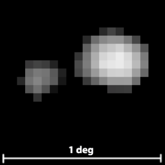
Figure 1: Image of 2E 1923.7+5037 and V* CH Cyg, left and right respectively. The sources are clearly separated by an angular distance of 29$\arcmin$. The sky–region is $\sim$1 $\times$ 1 deg² and the pixel size is 0.04 deg.

3 The SIX Survey: Results

3.1 Performance

3.1.1 Mosaic properties

The SIX survey covers 6200 deg². To study the quality of the mosaic image, we investigate its pixel distribution. The distribution is represented by the black solid line in Figure 2 where the red line is an overlaid Gaussian. Its mean value is 0 while the dispersion $\sigma$ = 1.0. At negative significances no wings are present. The long tail at positive significances represents real detected sources. The pixel-significance distribution demonstrates the quality of the background modeling.

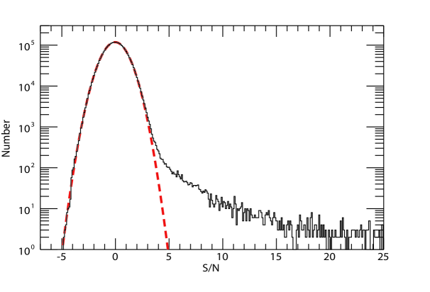
Figure 2: Pixel significance distribution of the SIX mosaic. The dashed line is an overlaid Gaussian with standard deviation $\sigma$ = 1.0. The distribution does not show any wings and the long tail at positive significances are real detected sources. (A color version of this figure is available in the online journal.)

3.1.2 Detection threshold

To identify an excess caused by a source in a mosaic image it is necessary to define the significance level at which the source population dominates over the noise distribution. To do so, we study the distribution of the pixel significances. In Figure 2 the largest negative fluctuation in the pixel distribution is found at $S/N=-4.8$. Taking into account the Gaussian distribution, we compute the number of pixels having the S/N-value above 4.8$\sigma$ not caused by the contribution of the sources but only due to statistical fluctuation. This is done by calculating the complementary error function. The value obtained is then multiplied by 0.5 since only positive fluctuations (the distribution’s tail at positive significances) can give rise to false detections. We then multiply this probability with the number of pixels ($\approx$ 3 $\times$ 10⁶). We find that only 2 pixels exceed the 4.8$\sigma$ detection threshold by chance.
The source search algorithm is based on the Swift/BAT standard tool batcelldetect. It uses the sliding cell method that detects a source at the position in the image where the signal of a pixel exceeds the background by our chosen detection threshold. However the oversampling of the BAT mosaic image might contribute to the fact that the detection threshold is exceeded by chance by the 2 pixels in the SIX mosaic. To avoid detecting such fluctuations as spurious sources, we require that at least 4 contiguous pixels exceed the detection threshold. Therefore, by setting the detection threshold to 4.8$\sigma$ we do not expect any false detection.

3.1.3 The SIX point spread function

We fit the SIX PSF to the region where the sources are detected. This results in accurate localization of the centroids of the sources. To determine the SIX PSF we have extracted the PSF of a large number of SIX sources without any preferred direction. This allows us to test the symmetry of the shape. The single source PSFs were normalized so that we can compute an overall mean PSF. The data points of the mean PSF are plotted in Figure 3 using open circles. The PSF profile can be modeled by a linear combination of the BAT PSF (dotted line) and the IBIS/ISGRI PSF (gray line). The BAT PSF (Markwardt et al., 2005) and the IBIS/ISGRI PSF (Gros et al., 2003) both have Gaussian shapes with standard deviations of 9.4$\arcmin$ and 5.1$\arcmin$ respectively. These values have been held fixed to perform a fit that minimizes $\chi$–square with $MINUIT$ (James & Roos, 1975). The normalization and mean values of both gaussians were free to vary. The resulting shape (black solid line in Figure 3) of the SIX PSF is symmetric with standard deviation of 6.8$\arcmin$. The derivation of the SIX PSF from linear combination of the PSFs of the single instruments resembles the method used to obtain the SIX mosaic image that is a linear combination of the sky maps of BAT and IBIS/ISGRI.

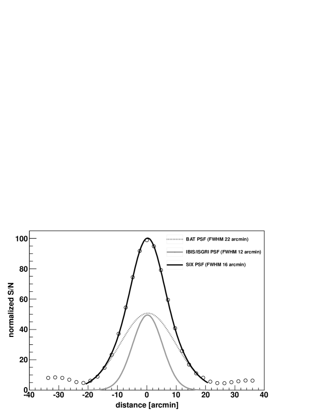
Figure 3: The SIX PSF (solid black line and FWHM 16$\arcmin$) is a linear combination of the BAT PSF (dotted gray line and FWHM 22$\arcmin$) and IBIS/ISGRI PSF (solid gray line and FWHM 12$\arcmin$).

3.1.4 Source flux

We extract from the SIX intensity map the fluxes of detected sources. The flux is computed by converting the count rate (cts) to physical units [erg cm^-2 s^-1] making use of the Crab as a calibration source:

$$\mathrm{F_{\rm SIX}\;[\rm erg\;cm^{-2}s^{-1}]=\left(\frac{F_{\rm SIX}\;[cts]}{F_{\rm Crab}\;[cts]}\right)F_{\rm Crab}\;[erg\;cm^{-2}s^{-1}]},$$ (8)

where the Crab flux in our survey band is given by

$$\mathrm{F}_{\rm Crab}=\int_{18keV}^{55keV}E\;F(E)\>dE.$$ (9)

The Crab spectrum F(E) in units of [photon cm^-2 sec^-1 keV^-1] is assumed to be power-law shaped having spectral index $\Gamma=-2.15$ and normalization factor $K=10.17$.

3.1.5 Sky coverage

The sky coverage allows one to get a first glance on the uniformity of the sensitivity over the surveyed sky region. The distribution of the sky area as function of detection limiting flux is therefore referred to as sky coverage. The sky coverage as a function of the minimum detectable flux $f_{min}$ is defined as the sum of the area covered to fluxes $f_{i}>f_{min}$:

$$\Omega(>f_{min})=\sum_{i}^{N}A_{i}\ \ \ \ f_{i}>f_{min}\ \ {\rm[deg^{2}]}$$ (10)

where $A_{i}$ is the area covered by each pixel and $N$ is the number of pixels. The minimum detectable flux $f_{min}$ is computed by multiplying the noise of the area associated to $A_{i}$ with the detection threshold.
As the SIX survey is the result of 2 independent surveys, we compute and study all 3 (IBIS/ISGRI, BAT, SIX) sky coverages. They are plotted in Figure 4, where the solid gray line, the dotted gray line and the solid black lines are the sky coverages of IBIS/ISGRI, BAT, and SIX respectively. It shows that BAT covers the entire surveyed sky area to a very uniform sensitivity reaching a flux limit of the order of $\sim$5 $\times$ 10^-12 erg cm^-2 s^-1. IBIS/ISGRI shows a varying sensitivity being very deep at the center of its mosaic image (limiting flux 4 $\times$ 10^-12 erg cm^-2 s^-1).

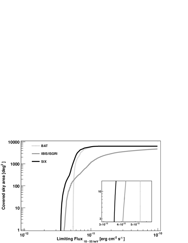
Figure 4: The sky coverages of IBIS/ISGRI (solid gray line), BAT (dotted gray line) and SIX (solid black line). The inset in the lower–right corner is a zoom–in at the level of limiting fluxes for the 3 surveys. The SIX sky coverage joins the best of IBIS/ISGRI and BAT being very uniform over the whole area and very deep in the center.

The difference between the two performances is mainly related to the different pointing strategies adopted by the two satellites. The main mission objective of Swift is to study Gamma-Ray Bursts (GRBs). While chasing up GRBs, Swift/BAT monitors the sky around the pointing directions. This permits having a uniform exposure and therefore a uniform sensitivity over the entire sky. INTEGRAL is a multiwavelengths observatory. It is the first of this kind. Its main objective is simultaneously observing objects in gamma–rays, hard and soft X-rays, and visible light. Therefore, INTEGRAL performs a pointed observing strategy, where the coordinates of the objects are known in advance. Around these coordinates INTEGRAL adopts a dither pattern. The dither pattern is a shift of the center of the instrument FOV with respect to the coordinates of the object that is being observed. The pattern consists of a rectangular 5 $\times$ 5 step with angular offset of 2.17^∘ and a small roll angle. As a consequence the innermost area (a few hundreds deg²) of our region of interest is continuously exposed to IBIS/ISGRI’s fully–coded FOV. This area exhibits the largest exposure time and therefore it is the sky area exhibiting the best sensitivity (see the IBIS/ISGRI exposure map in Figure 5). The extraneous area has a lower exposure time and it has a lower sensitivity. The SIX sky coverage joins the best of both (IBIS/ISGRI and BAT), being very sensitive and covering the surveyed area very uniformly at the same time. The whole survey is complete to a flux level of 10^-11 erg cm^-2 s^-1 while 50% of the SIX sky is surveyed to 8.5 $\times$ 10^-12 erg cm^-2 s^-1 and the best flux sensitivity is 3.3 $\times$ 10^-12 erg cm^-2 s^-1.

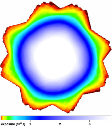
Figure 5: Color coded exposure map of IBIS/ISGRI on the NEP sky area. The innermost white region is the most exposed sky area corresponding to $\sim$180 deg². This corresponds in Figure 4 to the value on Y–axis where IBIS/ISGRI contributes most to the sensitivity limit of the survey. (A color version of this figure is available in the online journal.)

3.2 The SIX catalog

The SIX catalog (Table 5) contains 113 sources having S/N-ratio above 4.8$\sigma$. To identify this source sample we cross-correlate it with the BAT catalog (Ajello et al., 2008a; Cusumano et al., 2010), with the 4^th IBIS/ISGRI catalog (Bird et al., 2010), and with the INTEGRAL reference catalog . We have correlated our serendipitously detected objects also with the ROSAT All-Sky Survey Bright Source Catalogue (Voges et al., 1999). In addition, we have made use of the NASA/IPAC Extragalactic Database (NED) and the SIMBAD Astronomical Database. Positional queries were performed considering possible counterparts within a radius of 6$\arcmin$. We searched in literature for the absorption value (N_H) of each AGN. When not available, we have derived this parameter through the soft X-ray spectra. The soft X-ray data come from Chandra, Swift/XRT, and XMM-Newton observations. Chandra spectra were extracted using Chandra Interactive Analysis of Observations (CIAO: Fruscione et al., 2006) version 4.4. XMM-Newton Observation Data Files (ODFs) were processed using the XMM-Newton Scientific Analysis Software (SAS: Gabriel et al., 2004) version 10.0. We used Swift/XRT data in photon–counting mode only. For the analysis we used xrtproducts and HEAsoft 6.10.2. These instruments allow us to connect their spectra to the hard X-ray spectra since their upper energy threshold is between 6–10 keV, depending on the instrument. The joint fit of the soft X-ray and hard X-ray spectra of the same source allows derivation of the N_H value in excess to the Galactic column hydrogen density. This latter value was derived using the database accessible on–line and described in Kalberla et al. (2005). We used XSPEC 12 (Arnaud, 1996) and the latest available response matrices for calibration to perform the fit. The best model for the fit is given by an absorbed power–law with further absorption fixed to the Galactic column hydrogen density ($wabs(wabs*powerlaw)$). All the other parameters are free to vary. The N_H values and their references, when taken from literature, are reported in Table 5.
In addition, the redshifts of our sources are obtained by archive search of the counterparts. For these identified sources the rest–frame luminosity was computed in the 18–55 keV energy range using the equation

$$L_{18-55keV}=4\pi D_{L}^{2}\frac{F_{18-55}}{(1+z)^{2-\Gamma}}$$ (11)

where $\Gamma$ is the spectral index obtained from the spectral fit, F_18-55keV is the observed flux in the 18–55 keV energy range and $D_{L}$ is the luminosity distance.
We were able to identify 99 out of the 113 SIX sources, while 14 are unidentified. Among these 14 sources 7 are lacking soft X-ray counterparts, while 7 do not have any possible counterpart. Table 2 summarizes the types of sources detected in this survey. Roughly 16% of our AGN sample belongs to the blazar subclass. In their independent surveys IBIS/ISGRI finds 15% blazars (Foschini & Bianchin, 2008) as does BAT (Ajello et al., 2009). These results are in good agreement. For our blazar sample we have searched also for counter parts at gamma–ray energies. In order to find spatial coincidences we have cross–correlated the sky positions of our blazars with the source positions of the Second Fermi–LAT Catalog (2FGL: Ackermann et al., 2011). To account for the positional uncertainty of the Fermi–LAT sources, we find that the sources within 2$\sigma$ confidence level have an uncertainty $<$ 0.4 deg. Since the positional uncertainty of the SIX sources is smaller (6$\arcmin$), we search for spatial coincidences within a conservative error radius of 0.4 deg. We find that 10 of our blazars coincide with Fermi-LAT blazars.
The identified sources carry the information on the positional accuracy obtained in our survey. Making use of the sources with known X-ray counterpart, we report in Figure 6 the sources’ offset from their catalog positions as functions of the detection significances. The catalog position is derived from the position of the centroid of the SIX PSF that is fit to the region where the sources are detected. The result is that the SIX mosaic provides positions accurate to within $\sim$4$\arcmin$ for 95% of the sample. This is a very good location accuracy. A fit to the data shows that the mean offset varies as function of source significance accordingly to:

$$\textup{OFFSET}=(5.95\pm 0.28)\times(\textup{S/N})^{-0.38\pm 0.06}-(0.42\pm 0.29)\ \ \ \ {\rm[arcmin]}$$ (12)

A similar dependence on the source significance is known also for IBIS/ISGRI (Gros et al., 2003; Bird et al., 2006) as well as for BAT (Ajello et al., 2008a; Segreto et al., 2010). The absence of very bright sources in the SIX survey does not allow the fit in Figure 6 to be tightly constrained. However, we find that no SIX source is displaced by an offset larger than 6$\arcmin$ with respect to the SIMBAD or NED position. Therefore we can conclude that the SIX survey locates all sources to better than 6$\arcmin$.
As coded–mask detectors have a fairly poor angular resolution, we consider the possibility of source confusion. IBIS/ISGRI has a narrower PSF (12$\arcmin$) compared to that of BAT (22$\arcmin$). Resampling the BAT mosaic image to match the characteristics of the IBIS/ISGRI mosaic image does not affect the PSF of BAT. Therefore also the angular resolution of BAT is preserved in the resampled BAT image. Our new virtual instrument (the combination of BAT and IBIS/ISGRI) has an angular resolution of 16$\arcmin$ (see Figure 3), which is still a very good performance. Taking into account that the total surveyed sky area is 6200 deg² we end up with $\sim$48000 possible independent sky positions for the sources. If our surveyed sky area was covered uniformly to our limiting flux (3.3 $\times$ 10^-12 erg cm^-2 s^-1) then we would expect $\sim$1300 sources. Therefore, we can conclude that the source confusion is not an issue for this survey. In fact, the average source separation of our 113 SIX sources is $\sim$7^∘ on the 6200 deg² of sky area.

Table 2: Composition of the SIX Sample in the 18 – 55 keV Energy Band.

Class	Number of Objects
Seyfert-like AGN	74
Blazars	12
Galaxies	5
Galaxy clusters	2
Galactic sources	3
X-ray sources	3
Unidentified	14
Total	113

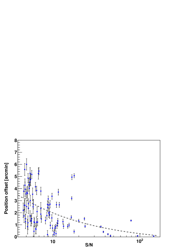
Figure 6: Offset from catalog position of sources detected in the SIX mosaic as function of S/N. The dashed line is the function described in Eq. 12. No sources have an offset larger than 6$\arcmin$.

3.3 Statistical properties

We use the results of our survey to derive cosmological information. Figure 7 shows the luminosity-redshift relation for the identified sources in the 18–55 keV energy band. Our flux–limited sample shows the clear trend where the most luminous sources are detected at the greatest distances. This is of particular importance as the flux–limited AGN sample spans a wide range in redshift. In Figure 7 black crosses represent Seyfert–like AGNs and red rectangles are blazars. Seyfert-like AGNs are sampled within 0 $<$ z $<$ 0.4. For z $>$ 0.4 only blazars are detected.

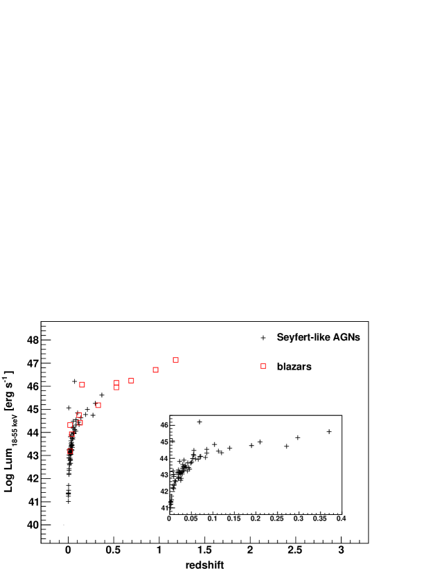
Figure 7: The redshift–luminosity plane shows our flux limited sample split into different source classes. Crosses are Seyfert–like AGN, while squares correspond to blazars. These latter sources are detected up to redshift $\sim$1.2. The inset in the lower right corner is a zoom–in into redshift range 0 $<$ z $<$ 0.4 where only values of Seyfert–like AGN are plotted. (A color version of this figure is available in the online journal.)

3.3.1 Source number–density

The log $N$–log $S$ relation represents a tool for detecting a possible cosmological evolution of a source class. For the SIX log $N$–log $S$ (see Figure 8) we assume a power–law form represented by: N($>$S) = K $\times$ S^α where $N$ is the number of sources above the source flux $S$. The best–fit to the differential log $N$–log $S$ is expressed by:

$$\mathrm{dN/dS}=(5.62\pm 0.65)\times 10^{-18}\;S^{2.38\pm 0.11}.$$ (13)

By integrating the differential function we obtain an Euclidean slope consistent with a non–evolving population in the local Universe. In case of evolution the value of $\alpha$ is expected to be greater than 1.5. We use the Seyfert–like AGNs reported in Ajello et al. (2009) and Krivonos et al. (2010) as control samples.

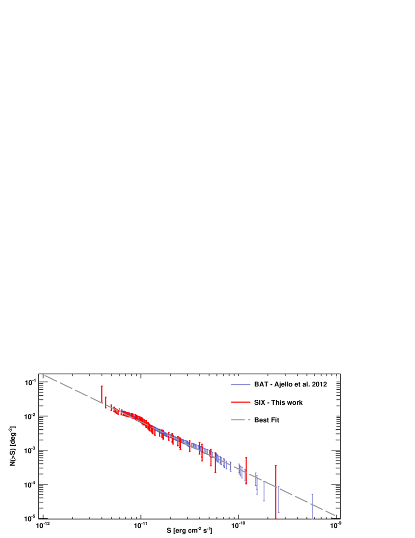
Figure 8: The cumulative log $N$–log $S$ distribution for our sample of AGN. For comparison the 60 months BAT sample (Ajello et al., 2012) is plotted in background. (A color version of this figure is available in the online journal.)

As expected, the power–law slopes agree well. The limiting flux in the SIX log $N$–log $S$ is a factor of $\sim$2 fainter and the number–density of sources is a factor of $\sim$4 higher. In general, the parameters used to model the number–density functions agree well. There is general consensus that the peak of the CXB is due to the integrated emission of unresolved Seyfert–like AGNs (La Franca et al., 2005; Gilli et al., 2007; Treister & Urry, 2005; Ueda et al., 2003; Silverman et al., 2008). Due to deep observations (Chandra Deep Field North, Chandra Deep Field South and XMM-Newton Lockman Hole) a detailed study of the CXB has been performed. The fraction of intensity due to AGN activity contributing to the CXB was found to decrease very rapidly with energy (Worsley et al., 2005). At its peak ($\sim$30 keV) less than 1% of the intensity of the CXB could be attributed to AGN activity (Ajello et al., 2008a). The contribution of the SIX-detected AGNs to the CXB is given by integrating the number–density $dN$/$dS$ multiplied by the source flux expressed as:

$$\mathrm{F}_{\rm diffuse}=\int_{18keV}^{55keV}dN/dS\;S\>dS=1.1356\times 10^{-9}\;{\rm erg\;cm^{-2}\;s^{-1}\;sr}$$ (14)

3.3.2 Luminosity and redshift dependence of the fraction of absorbed AGNs

As discussed in §1, the observations in the 18–55 keV energy band are very well suited for an unbiased (against absorption) detection of AGNs. We have derived the intrinsic $N_{H}$–value for 64 of our AGNs. In Figure 9 we show the histogram of the observed $N_{H}$ distribution (in units of number per bin). As an effective zero value, we set the column densities smaller than log $N_{H}$ $<$ 20 to log $N_{H}$ = 20. The histogram shows that the number of sources drops for column densities log $N_{H}$ $>$ 23. Roughly $\sim$3% of our Seyfert–like AGNs are Compton–thick.

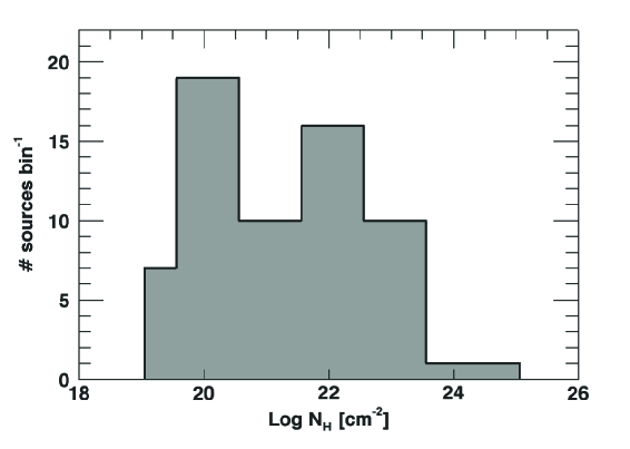
Figure 9: Distribution of intrinsic $N_{H}$–value inferred from soft X-ray observations.

Our sample covers a wide range in the $L_{X}-z$ plane. Thus, it is possible to constrain the luminosity dependence and the redshift dependence separately. Much attention has been paid to an observed anti–correlation of the fraction of absorbed AGNs as function of luminosity (e.g. Burlon et al., 2011, and references therein). Such a relation is at odds with the simple AGN unified model (Antonucci, 1993; Urry & Padovani, 1995) since the AGN properties are explained in terms of viewing angle and no other properties such as luminosity and/or accretion rate are involved. Scenarios have been proposed where obscuration due to the dust–sublimation radius depends on the luminosity ($R_{sub}\sim L^{0.5}$: Lawrence & Elvis, 1982) or where a misaligned disk with respect to the jet axis rules the obscuration (Lawrence & Elvis, 2010). But none of them are conclusive. In addition it seems that complex scenarios in the vicinity of the SMBH do not allow a simple interpretation of the observed anti–correlation. Considering that our $N_{H}$–inferred AGN sample is incomplete, we plot the faction of absorbed AGNs vs. luminosity (see Figure 10).

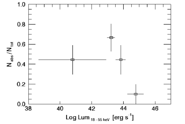
Figure 10: Fraction of obscured AGN (with log N_H $>$ 22) vs luminosity. The variables anti-correlate for luminosities $>$ 10⁴³ erg s^-1.

The reported errors are calculated as the 1 $\sigma$ binomial confidence interval as in Gehrels (1986). The fraction of the AGNs having log $N_{H}$ $>$ 22 decreases from 66% at $L_{X}$=43.2 erg s^-1 to 10% at $L_{X}$=44.7 erg s^-1. The widths of the luminosity ranges were chosen to contain the same number of sources. However, to draw conclusions on the shape and the drop of this relation a better statistic is needed. In this work the low statistics are due to the limited number of sources. Moreover, 10 AGNs are missing the $N_{H}$ measurement and 14 sources are without any counterpart.
Figure 11 shows the redshift dependence inferred from our sample. The statistical uncertainties are computed in the same way as for the luminosity dependence. Even though the uncertainties are rather large, a marginally-significant decay can be seen from our observations: the fraction of obscured AGNs declines from 55% at redshift $z=0.008$ to 22% at redshift $z=0.166$.

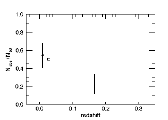
Figure 11: Fraction of obscured AGN (with log N_H $>$ 22) vs redshift.

3.3.3 The X-ray luminosity function

The X-ray luminosity functions (XLF) traces distribution and evolution of AGNs throughout the Universe. In turn this can give hints regarding the formation and growth of SMBHs and their fueling mechanisms. The SIX sample is well suited for this purpose because it has an adequate span in redshift and luminosity. We consider only those sources from the sample that are identified AGN. The AGN evolution and its quantification can be revealed using the $V/V_{MAX}$ method proposed in Schmidt (1968). Given a flux–limited survey and an object with constant luminosity, there is a maximum volume $V_{max}(z_{max})$ in which the object could have been detected. We compare $V_{max}(z_{max})$ and the volume in which the object was effectively detected $V_{z}$. Thus, this latter value can range from 0 to $V_{max}$. We can compute for each object $i$ the ratio $V_{i}/V_{imax}$. If the sample is complete and the source number–density constant within the co–moving volumes then $V_{i}/V_{imax}$ is uniformly distributed between 0 and 1, implying that the mean value $<$$V/V_{max}$$>$ = 0.5. Instead if the $<$$V/V_{max}$$>$ $\not=$ 0.5 then the objects are not uniformly distributed. For $<$$V/V_{max}$$>$ $>$ 0.5 a positive evolution in density or luminosity (or even both) is expected, while for $<$$V/V_{max}$$>$ $<$ 0.5 a negative evolution of the sample is expected. We find that $<$$V/V_{max}$$>$ = 0.49$\pm$0.02 implying the AGNs are not evolving in the local Universe. This result is in agreement with those reported in Tueller et al. (2008) and in Ajello et al. (2009).
The XLF is the co–moving number–density of AGNs having luminosities [$L,L+dL$]. We represent this function with a double power–law model as in Equation 15:

$$\Phi(L_{X},z=0)=\frac{d^{2}N}{dVdL_{X}}=\frac{K}{ln(10)L_{X}}\left[\left(\frac{L_{X}}{L_{*}}\right)^{\gamma_{1}}+\left(\frac{L_{X}}{L_{*}}\right)^{\gamma_{2}}\right]^{-1}$$ (15)

where $\gamma_{1}$ is the low-end slope, $\gamma_{2}$ is the high-end slope, $K$ is a normalization factor including the overall density, and $L_{*}$ is the break luminosity. The best-fit parameters are reported in Table 3. A visual representation of the XLF in shown in Figure 12. The data points are plotted together with their horizontal and vertical error bars. The best–fit is obtained by applying the model of Equation 15. For comparison we plot the fit result obtained by Ajello et al. (2012) who used the same model applied to the BAT sample alone. Furthermore we compare our result with the results of previous works (Beckmann et al., 2006; Sazonov et al., 2007; Tueller et al., 2008; Ajello et al., 2009) performed at hard X-ray energies although not exactly in the same energy range. The low-end slope, the high-end slope, and the break-luminosity agree well.

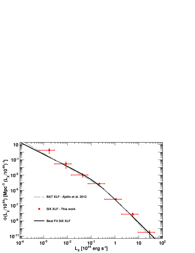
Figure 12: Luminosity function of Seyfert-like AGNs detected in the SIX survey. The data (dots with error bars) are represented by a non-evolving double power-law model (black solid line). Parameters are reported in Table 3. For comparison the same model for the BAT-detected (gray dashed line) sources is plotted. (A color version of this figure is available in the online journal.)

Table 3: XLF in the Energy Range 18–55 keV: Best-fit Parameters

Ka	$\gamma_{1}$	$\gamma_{2}$	$L_{*}^{b}$
6.13$\pm$0.71	0.57$\pm$0.08	2.07$\pm$0.16	0.17$\pm$0.07

^ain units of 10^-5 erg^-1 s Mpc^-3
bin units of 10⁴⁴ erg s^-1

4 Discussions

4.1 The SIX: the survey of a virtual new X-ray mission

To capitalize on the advantages of selecting local AGNs at hard X-ray energies we have combined the observations of IBIS/ISGRI and BAT. This greatly enhances the exposure time improving the SIX sensitivity as $t_{exposure}^{-0.5}$. Moreover, the systematic uncertainties are minimized because the systematic errors of both instruments are uncorrelated. This reduces the uncertainties by a covariance term leading to a limiting flux sensitivity of 3.3 $\times$ 10^-12 erg cm^-2 s^-1 in the 18–55 keV energy range.
BAT contributes to the SIX survey with a very uniform exposure. The exposure of IBIS/ISGRI is less uniform (see Figure 4). This is explained by the different FOVs of both coded–masks instruments and by the different pointing strategies that are adopted by the Swift and the INTEGRAL missions. INTEGRAL performs a dithering that leads to a large exposure time at the center of the surveyed sky area as shown in Figure 5. The center of this sky area corresponds roughly to the value of the ordinate in Figure 4 where the IBIS/ISGRI sky coverage outperforms that of BAT. IBIS/ISGRI is therefore contributing to the SIX survey with its long exposures on limited sky areas.

4.2 Results from the sample

From observations at soft X–rays we have inferred the $N_{H}$-value of 64 out of our 74 AGNs. The level of this incompleteness will change as some of these sources are followed up by Chandra (PI E. Bottacini CXC AO-13) and XRT. The fraction of obscured AGNs as function of luminosity is consistent with a previous work (Burlon et al., 2011). Also the drop at low luminosities $\sim$10⁴³ erg s^-1 is reproduced in our work. The relation is represented by an anti–correlation shown in Figure 10 revealing that the $N_{H}$ function is luminosity dependent. In contrast to the simple AGN unified scheme (Antonucci, 1993; Urry & Padovani, 1995), where AGNs have the same geometrical structure irrespective of luminosity and redshift, this result shows that the opening angle of the torus surrounding the SMBH is larger for more luminous AGNs. Therefore, high–luminosity AGNs must be able to ’clean out’ their environments. The physical process responsible for this could be the stronger radiation pressure from the SMBH of the more luminous AGNs. In this scenario the circumnuclear environment is exposed to higher pressure that causes greater mass outflow. Indeed, the existence of such mass outflows is supported by recent observations (Pounds & Reeves, 2009; Sturm et al., 2011; Rupke & Veilleux, 2011). If accompanied by sufficient mechanical energy transfer, these outflows can provide the coupling of the SMBH and host galaxy co-evolution (Pounds & Reeves, 2009). However, it is ambitious to draw conclusions from the observational fact of the anti–correlation. How the covering factor of the torus relates to the luminosity depends on the interplay of the SMBH gravity with the gas, radiation, and magnetic fields accompanied by wind outflows. The thermal pressure in the gas is able to explain the low-velocity outflow as X-ray warm absorbers (Krolik & Kriss, 2001). Instead, the UV radiatively-driven wind shields itself from X-rays from the central engine (Murray & Chiang, 1995). On the other hand, a natural shielding is obtained in the magneto-centrifugal outflow scenario (Everett, 2005). Finally, in hydrodynamical simulations (Proga & Kallman, 2004) high-density gas arises naturally that is able to efficiently absorb X-ray radiation. All these processes show promising results in numerical simulations.
A possible dependence (decrease) of the fraction of absorbed AGNs as function of redshift is marginally detected in this work (see Figure 11). Even though within a larger redshift (z $<$ 3) range, a similar relation is found by Ueda et al. (2003). Instead a strong increase of the fraction of obscured AGN within 0 $<$ z $<$ 2 is found by La Franca et al. (2005) and Hasinger (2008). This dependency on the distance at high redshift can be due to the higher gas content in high–redshift (z $\sim$ 1.5) galaxies (Daddi et al., 2010). In the local Universe our results show a mild decay of the fraction of obscured AGNs with redshift.
The fit to our flux–number density function is consistent with the Euclidean model. This is in good agreement with previous measurements by Krivonos et al. (2005), Beckmann et al. (2006), Tueller et al. (2008), and Ajello et al. (2009). We extend the result towards lower fluxes reaching a flux limit of a few 10^-12 cm^-2 s^-1. As a result of the increase of the number density of sources, the SIX source sample improves the number–density of sources contributing to the CXB by more than a factor $\sim$ 2 compared to the fraction derived from the sample in Ajello et al. (2009). The contribution of the latter sample to the CXB is obtained by integrating the emission of the AGN over the entire extragalactic sky of 30000 deg². Even though in our work we survey $\sim$1/5 of the extragalactic sky, our surveyed sky area is particularly suited because of absence of strong sources. We can estimate the number of Seyfert–like AGN in a deep NuSTAR (Harrison et al., 2010) survey. NuSTAR is a NASA mission operating at energies in the range 3–80 keV and scheduled to be launched in June 2012. It is the first high energy X-ray mission using focusing optics. Its relatively small FOV ($\sim$ 13 $\times$ 13 arcmin squared) allows surveying small areas compared to coded–mask detectors. If the luminosity function derived here does not evolve strongly in either normalization and/or slope the estimated number of AGN per square degree at energies $\sim$30 keV is $\sim$100 for a limiting flux of 10^-14 erg cm^-2 s^-1. This will be quite possible to be performed by NuSTAR since it will have an angular resolution $\sim$45 arc sec and source confusion will not be a problem. NuSTAR will perform very sensitive and beam–like extragalactic surveys tiling not more than a few deg² of sky area. Detailed predictions (Ballantyne et al., 2011) show, that independent of NuSTAR’s survey strategy (corner shift or half shift) and the CXB models, AGNs will be sampled most efficiently at redshift z $>$ 0.5. Figure 13 displays the redshift - luminosity plane of Seyfert-like AGNs sampled by BAT (gray circles in background from Ajello et al., 2009), SIX (solid circles in foreground), and NuSTAR. NuSTAR data are taken from predictions in Ballantyne et al. (2011) and adapted to the energy range 18–55 keV.

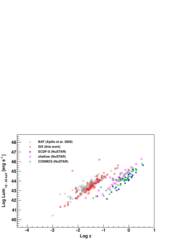
Figure 13: Luminosity-redshift plane of the BAT (gray circles in background) sample, SIX sample (red circles in foreground), and predicted NuSTAR samples for different sky areas (Ballantyne et al., 2011). (A color version of this figure is available in the online journal.)

As the NuSTAR survey fields narrow, the redshift distribution of AGNs is shifted to higher redshift. This is shown in Figure 13 where squares are from a shallow survey, crosses from the COSMOS survey (2 deg²), and asterisks from the ECDF-S survey (0.25 deg²) assuming an exposure of 6.2 Msec. NuSTAR’s surveys will not compete with the SIX survey, but rather they will be complementary. Indeed, if applied to the whole sky the SIX survey will fill the redshift and luminosity gap between the current surveys of IBIS/ISGRI and BAT alone and the NuSTAR surveys. The absorbed SIX sources at low redshift are easy follow up targets for NuSTAR.
Our small sample used for the XLF does not permit detecting an evolution in either luminosity or redshift. Therefore, our data are modeled best by a non-evolving XLF plotted in Figure 12.
We use the 199 BAT-selected Seyfert-like AGNs of Ajello et al. (2009) and later used in Burlon et al. (2011) as a control sample in order to evaluate whether the SIX sample differs in some properties. For both samples we have derived the redshift distribution excluding radio-loud AGNs and quasars. The result is plotted in Figure 14 where the solid line refers to the SIX sample and the dashed line represents the sample of Ajello et al. (2009). Both samples were split into the same bin size. About 57% of the BAT sources are detected within z = 0–0.025. In the same redshift bin the SIX survey samples less than 45% of its sources.

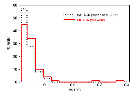
Figure 14: Redshift distribution of the BAT sample (dashed line) and the SIX sample (solid line). The SIX survey samples the sources systematically at higher redshift compared to the BAT survey. (A color version of this figure is available in the online journal.)

The SIX survey is more sensitive compared to the BAT survey. Therefore it samples the sources systematically at higher redshift. Sources at higher redshift are also the most luminous ones. This is marginally reflected in the XLF (see Figure 12) for luminosities above $10^{45}\;erg\;s^{-1}$. The best-fit of the XLF adapted from the BAT survey (dashed line) has a slightly steeper slope at high luminosities. For luminosities below $10^{42}\;erg\;s^{-1}$ a substantial contribution from the host galaxy to the total luminosity is expected. Therefore, the data point at lowest luminosities in not properly modeled by the SIX XLF.
Finally, we verify whether the control samples and the SIX sample are drawn from the same source population. A Kolmogorov-Smirnov test applied to the two samples with respect to redshift and luminosity does not allow us to reject the null hypothesis that the two samples are obtained from the same source population. Therefore, the SIX is sampling sources at higher redshift from the same source population that is sampled by BAT alone. Better statistics for the SIX XLF can rule out the high-end slope. This can be achieved by applying the survey to the whole sky.

5 Conclusions

A new approach has been developed to survey the sky at hard X-ray energies (18–55 keV energy band) by combining the observations of Swift/BAT and INTEGRAL/IBIS resulting in the SIX survey. First we have performed the independent surveys for both instruments. Then we have resampled, cross-calibrated and merged them. As a result of combining the observations from two different telescopes, statistical and systematic uncertainties caused by the high background level of their coded-mask detectors are minimized. In turn the SIX survey is more sensitive, like a survey from a virtual new hard X-ray mission.
We applied the survey method to 6200 deg² of sky ($\sim$ 20% of the entire extragalactic sky) sampling 113 sources that are: 74 Seyfert-like AGNs, 12 blazars, 5 galaxies, 2 clusters of galaxies, 3 Galactic sources, 3 previously detect X-ray sources, and 14 unidentified sources (of which 7 are newly detected without any counterpart and 7 are of uncertain association). No false detections due to statistical or systematic fluctuations are expected. The sources are identified through their soft X-ray counterparts and with Chandra follow up observations (CXC AO-12). Unidentified sources are being followed-up in Chandra AO-13. Among the AGN sample only two sources are Compton–thick, accounting for $\sim$3% of the entire sample.
The number density of our identified sources is $\sim$4 times greater than in our control sample of Ajello et al. (2009). Even though this represents only a minor fraction of the CXB, the sensitivity improvement with respect to previous measurements is better than a factor of 2.
The fraction of absorbed AGN decreases with increasing luminosities. Although the redshift dependence is marginally significant, we find a mild decrease of the fraction of obscured AGNs with increasing redshift. These results require that the covering factor of the torus surrounding the SMBH changes at least with luminosity.
Only robustly identified AGNs were used in our XLF. The data are well represented by a double power-law model and do not show any evolution in density or in luminosity. The non-evolving XLF model fits our data best.
Based on our results we predict the number density of $\sim$100 Seyfert–like AGNs that the upcoming NuSTAR mission can detect in 1 deg² of surveyed sky area at a limiting flux of $10^{-14}\;erg\;cm^{-2}\;s^{-1}$.

Table 4: Detected Hard X-Ray Sources

R.A.	Decl.	Counterpart	Flux	S/N	Obj Class	Obj Type	Redshift	Luminosity	log $N_{H}$
(J2000)	(J2000)		(10-12 erg cm-2 s-1)				(z)	(erg s-1)	(cm-2)
133.8152	64.4063	MCG+11-11-032	7.97	6.44	AGN	Sy2	0.03	43.40	23.01 [1]
148.9211	69.6846	M 82	7.09	4.90	galaxy interacting	galaxy interacting	0.0006	39.97	$\cdots$
149.0083	69.0811	M 81	10.1	7.34	AGN	LINER	0.0001	38.64	20.53 [1]
150.4723	55.6943	4C 55.19	13.9	11.4	AGN	Sy2	0.004	41.64	24.7 [2]
161.0304	70.4238	MCG+12-10-067	6.31	5.67	AGN	Sy2	0.03	43.20	23.29 [1]
163.2331	10.6582	$\cdots$	11.6	6.67	$\cdots$	$\cdots$	$\cdots$	$\cdots$	$\cdots$
166.1311	38.2082	Mrk 421	101.	78.5	blazar	BL Lac	0.02	44.32	$\cdots$
166.4922	58.9187	1RXS J110537.4+585128	5.66	5.04	AGN	QSO	0.19	44.77	21.20 [1]
166.6683	72.5697	NGC 3516	57.8	46.0	AGN	Sy1.5	0.00	42.99	21.21 [1]
168.9601	54.4453	$\cdots$	6.31	4.80	$\cdots$	$\cdots$	$\cdots$	$\cdots$	$\cdots$
171.3510	54.3702	Mrk 0040	10.7	9.16	AGN	Sy1	0.02	43.01	20.90 [2]
172.5265	-14.817	OM -146	17.4	8.96	blazar	FSRQ	1.18	47.14	$\cdots$
173.1405	52.9792	NGC 3718	7.10	6.89	AGN	LINER	0.003	41.23	20.00 [2]
173.2427	10.2765	2MASX J11324928+1017473	7.57	5.99	AGN	Sy1	0.04	43.52	21.46 [1]
174.2112	67.6433	RBS 1004	5.50	5.42	blazar	BL Lac	0.13	44.42	$\cdots$
174.8026	59.2078	RBS 1011	11.2	9.43	AGN	Sy1.5	0.06	43.98	19.58 [3]
175.5590	10.3157	NGC 3822	5.85	5.60	AGN	Sy1	0.02	42.88	20.00 [1]
175.9280	71.6968	DO Dra	15.2	10.6	CV	V* DO Dra	$\cdots$	$\cdots$	$\cdots$
176.3579	58.9892	MCG+10-17-061	8.39	6.15	galaxy	galaxy	0.01	42.30	$\cdots$
176.4277	-18.436	RBS 1030	31.5	15.4	AGN	Sy1	0.03	43.89	20.54 [1]
177.0379	9.00302	2MASX J11475508+0902284	8.07	5.24	AGN	Sy?	0.06	43.96	21.00 [1]
178.0421	-11.374	RBS 1044	10.3	5.52	AGN	Sy1	0.04	43.76	$\cdots$
178.4084	49.5092	RBS 1046	4.13	4.82	blazar	FSRQ	0.33	45.18	$\cdots$
179.5145	55.4250	NGC 3998	9.91	7.43	AGN	LINER	0.003	41.46	20.09 [1]
179.6989	42.5570	IC 751	4.36	5.90	AGN	Sy2	0.03	43.00	$\cdots$
180.1644	-1.1668	2QZ J120045.2-011041	10.1	6.73	AGN	Sy1	0.37	45.67	$\cdots$
180.2348	6.81394	CGCG 041-020	11.8	9.36	AGN	Sy2	0.03	43.54	22.83 [3]
180.2905	-3.6918	Mrk 1310	5.67	5.34	AGN	Sy1	0.01	42.69	20.72 [1]
180.7713	44.5210	NGC 4051	25.4	23.5	AGN	Sy1.5	0.002	41.41	20.47 [1]
181.5795	52.7170	NGC 4102	10.8	10.4	AGN	LINER	0.002	41.29	20.94 [1]
182.2920	47.0460	Mrk 0198	8.73	8.30	AGN	Sy2	0.02	43.07	22.80 [1]
182.3597	43.6981	NGC 4138	11.3	11.2	AGN	Sy1.9	0.002	41.33	22.90 [3]
182.6350	39.4063	NGC 4151	239.	222.	AGN	Sy1	0.003	42.74	22.50 [3]
182.6950	38.3332	KUG 1208+386	11.8	6.88	AGN	Sy1	0.02	43.14	22.53 [2]
183.0916	-7.5984	$\cdots$	9.56	6.69	$\cdots$	$\cdots$	$\cdots$	$\cdots$	$\cdots$
183.2574	7.03921	2MASS J12124981+0659451	7.99	6.37	AGN	QSO	0.20	45.00	$\cdots$
184.2881	7.17577	NGC 4235	12.3	9.99	AGN	Sy1	0.007	42.21	21.16 [1]
184.7378	47.2874	NGC 4258	11.3	10.7	AGN	LINER	0.001	40.77	22.91 [4]
185.5332	75.3006	Mrk 205	11.9	8.60	AGN	Sy1	0.07	44.15	20.88 [5]
185.6009	4.20212	4C 04.42	10.5	9.81	blazar	FSRQ	0.96	46.70	$\cdots$
185.8403	2.68141	Mrk 50	12.8	8.75	AGN	Sy1	0.02	43.19	20.92 [1]
186.4482	12.6643	NGC 4388	119.	94.0	AGN	Sy2	0.008	43.27	23.63 [3]
187.2817	2.04932	3C 273	172.	143.	blazar	FSRQ	0.15	46.07	$\cdots$
188.6686	52.6444	$\cdots$	6.42	5.11	$\cdots$	$\cdots$	$\cdots$	$\cdots$	$\cdots$
189.6855	9.46984	2MASX J12384342+0927362	6.61	5.66	AGN	Sy2	0.08	44.05	$\cdots$
189.7676	-16.184	IGR J12391-1612	16.8	10.9	AGN	Sy2	0.03	43.72	22.48 [1]
189.9053	-5.3471	NGC 4593	42.2	38.1	AGN	Sy1	0.009	42.88	20.30 [3]
191.7000	54.5375	NGC 4686	9.72	9.24	AGN	Sy2	0.01	42.78	23.84 [1]
192.8286	-11.722	$\cdots$	9.22	5.81	$\cdots$	$\cdots$	$\cdots$	$\cdots$	$\cdots$
193.0649	-13.419	NGC 4748	9.34	6.18	AGN	Sy1	0.01	42.59	20.77 [1]
193.9939	4.33340	$\cdots$	5.84	5.21	$\cdots$	$\cdots$	$\cdots$	$\cdots$	$\cdots$
194.0513	-5.7909	3C 279	12.4	10.3	blazar	FSRQ	0.53	46.15	$\cdots$
195.9917	53.7738	IGR J13038+5348	16.4	14.9	AGN	Sy1	0.02	43.52	20.81 [1]
196.0532	-5.5644	NGC 4941	9.11	6.45	AGN	Sy2	0.003	41.43	22.95 [1]
196.0877	-10.309	NGC 4939	12.0	8.75	AGN	Sy2	0.01	42.46	$\cdots$
196.9632	-2.0556	$\cdots$	7.63	7.48	$\cdots$	$\cdots$	$\cdots$	$\cdots$	$\cdots$
197.2785	11.6407	NGC 4992	20.9	17.6	AGN	Sy2	0.02	43.48	23.74 [6]
198.2996	-11.127	RBS 1233	8.95	6.65	AGN	Sy1	0.03	43.38	20.74 [1]
198.8493	44.4093	Mrk 248	11.3	11.4	AGN	Sy2	0.03	43.51	22.81 [2]
199.7661	-9.3549	$\cdots$	6.85	5.89	$\cdots$	$\cdots$	$\cdots$	$\cdots$	$\cdots$
200.2616	8.96113	NGC5100	6.13	5.29	galaxy group	galaxy group	0.03	43.15	$\cdots$
200.6131	-16.733	MCG-03-34-063	21.3	11.0	AGN	Sy2	0.01	43.12	23.59 [3]
202.1334	-1.5129	$\cdots$	6.34	5.36	$\cdots$	$\cdots$	$\cdots$	$\cdots$	$\cdots$
203.6978	-23.425	ESO 509-66	13.2	5.77	AGN	Sy2	0.04	43.79	23.05 [1]
203.9518	3.01973	NGC 5231	8.80	5.29	AGN	$\cdots$	0.02	42.97	22.23 [1]
204.3828	-13.032	QSO B1334-127	7.91	4.83	blazar	BL Lac	0.53	45.95	$\cdots$
204.5677	4.54615	NGC 5252	52.1	43.0	AGN	Sy2	0.02	43.76	22.34 [8]
205.0111	55.8247	$\cdots$	8.60	5.48	$\cdots$	$\cdots$	$\cdots$	$\cdots$	$\cdots$
205.3109	-14.660	RBS 1303	13.0	6.54	AGN	Sy1	0.04	43.72	21.23 [1]
206.3981	41.6618	NGC 5290	9.73	5.77	galaxy group	galaxy group	0.00	42.20	$\cdots$
208.0023	-18.300	$\cdots$	16.9	6.12	$\cdots$	$\cdots$	$\cdots$	$\cdots$	$\cdots$
208.3393	69.3013	Mrk 279	21.0	16.3	AGN	Sy1	0.03	43.65	20.53 [3]
208.4456	-11.406	$\cdots$	7.69	4.80	$\cdots$	$\cdots$	$\cdots$	$\cdots$	$\cdots$
209.0421	38.5687	Mrk 0464	10.2	8.91	AGN	Sy1	0.05	43.79	20.00 [2]
213.3866	-3.2043	NGC 5506	131.	79.0	AGN	Sy1.9	0.00	43.03	22.53 [3]
215.4348	47.7875	RBS 1378	10.4	9.36	AGN	Sy1	0.07	44.11	21.26 [2]
216.5659	37.8241	ABELL 1914	5.11	5.16	galaxy cluster	galaxy cluster	0.17	44.61	$\cdots$
217.2120	42.6515	H 1426+428	13.0	11.6	blazar	BL Lac	0.12	44.75	$\cdots$
217.3623	1.31454	Mrk 1383	12.2	6.97	AGN	Sy1	0.08	44.35	20.00 [2]
218.4907	5.47754	NGC 5674	8.13	5.55	AGN	Sy1	0.02	43.06	$\cdots$
218.8075	48.6441	NGC 5683	6.77	5.09	AGN	Sy1	0.04	43.42	$\cdots$
219.1769	58.7837	Mrk 817	15.5	11.9	AGN	Sy1	0.03	43.54	23.49 [2]
219.3705	58.9051	$\cdots$	8.57	7.18	$\cdots$	$\cdots$	$\cdots$	$\cdots$	$\cdots$
220.2547	53.4781	Mrk 477	9.68	7.34	AGN	Sy2	0.03	43.51	24.00 [7]
220.6846	-17.225	NGC 5728	42.2	17.6	AGN	Sy2	0.01	42.92	24.14 [9]
228.8484	42.0416	NGC 5899	8.82	6.56	AGN	Sy2	0.01	42.15	23.12 [2]
229.8817	65.6329	MCG+11-19-006	7.33	4.91	AGN	Sy2	0.04	43.52	21.38 [1]
234.0596	57.8813	Mrk 290	13.0	9.86	AGN	Sy1	0.02	43.41	20.40 [3]
236.6410	69.4657	2MASX J15462424+6929102	5.66	5.17	galaxy	galaxy	$\cdots$	$\cdots$	$\cdots$
243.5509	65.6973	Mrk 876	8.32	6.02	AGN	Sy1	0.11	44.49	19.06 [1]
245.0576	81.0390	MCG+14-08-004	10.4	8.79	AGN	Sy2	0.02	43.13	22.88 [1]
247.1031	51.7736	Mrk 1498	23.9	16.5	AGN	Sy1.9	0.05	44.24	23.26 [3]
253.1046	55.9419	MCG+09-28-001	5.49	4.83	AGN	Sy2	0.02	43.02	22.66 [1]
259.9293	48.9820	Arp 102B	10.7	5.47	blazar	FSRQ	0.02	43.18	$\cdots$
260.5280	43.2471	FIRST J172201.9+431523	9.15	5.05	AGN	Sy1	0.13	44.67	21.12 [1]
270.0433	66.5841	NGC 6552	4.98	4.96	AGN	Sy2	0.02	42.90	$\cdots$
274.0939	49.8605	AM Her	35.0	23.1	CV	CV	$\cdots$	$\cdots$	$\cdots$
275.5807	64.3694	1ES 1821+643	7.00	9.06	AGN	Sy1	0.29	45.29	20.00 [2]
277.5011	48.7652	3C 380	8.34	5.58	blazar	$\cdots$	0.69	46.24	$\cdots$
280.6068	79.7714	3C 390.3	39.8	35.7	AGN	Sy1	0.05	44.47	21.03 [3]
281.3777	72.1933	2MASX J18452628+7211008	3.97	5.22	AGN	Sy2	0.04	43.29	22.82 [1]
290.2788	43.9628	ACO 2319	24.2	16.6	galaxy cluster	galaxy cluster	0.05	44.25	$\cdots$
291.1899	50.2373	CH Cyg	11.8	7.33	symbiotic star	symbiotic star	$\cdots$	$\cdots$	$\cdots$
291.2818	50.6906	2E 1923.7+5037	7.98	4.92	X-ray source	X-ray source	$\cdots$	$\cdots$	$\cdots$
291.7341	41.5856	1RXS J192630.6+413314	10.8	5.53	X-ray source	X-ray source	$\cdots$	$\cdots$	$\cdots$
292.1210	73.9471	1ES 1928+73.8	5.32	4.98	AGN	Sy1	0.03	43.20	20.93 [1]
296.8676	44.8043	CXOU J194719.3+444942	13.8	9.04	AGN	Sy2	0.05	43.96	$\cdots$
299.7378	40.8185	CXO J195857.9+404856	38.2	31.4	X-ray source	X-ray source	$\cdots$	$\cdots$	$\cdots$
300.0223	65.1576	1ES 1959+650	15.5	13.3	blazar	BL Lac	0.04	43.92	$\cdots$
310.7268	75.1344	4C 74.26	25.0	19.9	AGN	Sy1	0.10	44.83	21.22 [1]
311.7313	65.2038	$\cdots$	5.67	4.81	$\cdots$	$\cdots$	$\cdots$	$\cdots$	$\cdots$
318.6292	82.0649	S5 2116+81	19.2	13.1	AGN	Sy1	0.08	44.54	21.03 [1]
337.3319	66.7884	IGR J22292+6647	11.2	6.12	AGN	Sy?	0.11	44.56	21.77 [1]

References. — [1] this work; [2] Burlon et al., 2011; [3] Tueller et al., 2008; [4] Cappi et al., 2006; [5] Page et al., 2005; [6] Winter et al., 2008; [7] Shu et al., 2007; [8] Dadina et al., 2010; [9] Comastri et al., 2010.

References

- Ackermann et al. (2011) Ackermann, M. et al. 2011, ApJ, 743, 171
- Ajello et al. (2012) Ajello, M., Alexander, D. M., Greiner, J., Madejski, G. M., Gehrels, N., & Burlon, D. 2012, ApJ, 749, 21
- Ajello et al. (2009) Ajello, M. et al. 2009, ApJ, 699, 603
- Ajello et al. (2008a) Ajello, M., Greiner, J., Kanbach, G., Rau, A., Strong, A. W., & Kennea, J. A. 2008a, ApJ, 678, 102
- Ajello et al. (2008b) Ajello, M. et al. 2008b, ApJ, 689, 666
- Ajello et al. (2008c) —. 2008c, ApJ, 673, 96
- Alexander et al. (2003) Alexander, D. M. et al. 2003, AJ, 126, 539
- Alonso-Herrero et al. (2006) Alonso-Herrero, A. et al. 2006, ApJ, 640, 167
- Antonucci (1993) Antonucci, R. 1993, ARA&A, 31, 473
- Arnaud (1996) Arnaud, K. A. 1996, in Astronomical Society of the Pacific Conference Series, Vol. 101, Astronomical Data Analysis Software and Systems V, ed. G. H. Jacoby & J. Barnes, 17
- Ballantyne et al. (2011) Ballantyne, D. R., Draper, A. R., Madsen, K. K., Rigby, J. R., & Treister, E. 2011, ApJ, 736, 56
- Barthelmy et al. (2005) Barthelmy, S. D. et al. 2005, Space Science Reviews, 120, 143
- Beckmann et al. (2006) Beckmann, V., Soldi, S., Shrader, C. R., Gehrels, N., & Produit, N. 2006, ApJ, 652, 126
- Bird et al. (2006) Bird, A. J. et al. 2006, ApJ, 636, 765
- Bird et al. (2010) —. 2010, ApJS, 186, 1
- Boella et al. (1997) Boella, G., Butler, R. C., Perola, G. C., Piro, L., Scarsi, L., & Bleeker, J. A. M. 1997, A&AS, 122, 299
- Bottacini et al. (2010) Bottacini, E., Böttcher, M., Schady, P., Rau, A., Zhang, X., Ajello, M., Fendt, C., & Greiner, J. 2010, ApJ, 719, L162
- Brandt et al. (2001) Brandt, W. N. et al. 2001, AJ, 122, 2810
- Brandt & Hasinger (2005) Brandt, W. N., & Hasinger, G. 2005, ARA&A, 43, 827
- Burlon et al. (2011) Burlon, D., Ajello, M., Greiner, J., Comastri, A., Merloni, A., & Gehrels, N. 2011, ApJ, 728, 58
- Cappelluti et al. (2009) Cappelluti, N. et al. 2009, A&A, 497, 635
- Cappi et al. (2006) Cappi, M. et al. 2006, A&A, 446, 459
- Comastri et al. (2007) Comastri, A., Gilli, R., Vignali, C., Matt, G., Fiore, F., & Iwasawa, K. 2007, Progress of Theoretical Physics Supplement, 169, 274
- Comastri et al. (2010) Comastri, A., Iwasawa, K., Gilli, R., Vignali, C., Ranalli, P., Matt, G., & Fiore, F. 2010, ApJ, 717, 787
- Courvoisier et al. (2003) Courvoisier, T. J.-L. et al. 2003, A&A, 411, L53
- Cusumano et al. (2010) Cusumano, G. et al. 2010, A&A, 524, A64+
- Daddi et al. (2010) Daddi, E. et al. 2010, ApJ, 713, 686
- Dadina et al. (2010) Dadina, M., Guainazzi, M., Cappi, M., Bianchi, S., Vignali, C., Malaguti, G., & Comastri, A. 2010, A&A, 516, A9
- Di Cocco et al. (2003) Di Cocco, G. et al. 2003, A&A, 411, L189
- Donley et al. (2007) Donley, J. L., Rieke, G. H., Pérez-González, P. G., Rigby, J. R., & Alonso-Herrero, A. 2007, ApJ, 660, 167
- Everett (2005) Everett, J. E. 2005, ApJ, 631, 689
- Fadda et al. (2002) Fadda, D., Flores, H., Hasinger, G., Franceschini, A., Altieri, B., Cesarsky, C. J., Elbaz, D., & Ferrando, P. 2002, A&A, 383, 838
- Foschini & Bianchin (2008) Foschini, L., & Bianchin, V. 2008, in PoS, Proceedings of the 7th INTEGRAL Workshop, 49
- Frontera et al. (1997) Frontera, F., Costa, E., dal Fiume, D., Feroci, M., Nicastro, L., Orlandini, M., Palazzi, E., & Zavattini, G. 1997, in Society of Photo-Optical Instrumentation Engineers (SPIE) Conference Series, Vol. 3114, Society of Photo-Optical Instrumentation Engineers (SPIE) Conference Series, ed. O. H. Siegmund & M. A. Gummin, 206–215
- Fruscione et al. (2006) Fruscione, A. et al. 2006, in Society of Photo-Optical Instrumentation Engineers (SPIE) Conference Series, Vol. 6270, Society of Photo-Optical Instrumentation Engineers (SPIE) Conference Series
- Gabriel et al. (2004) Gabriel, C. et al. 2004, in Astronomical Society of the Pacific Conference Series, Vol. 314, Astronomical Data Analysis Software and Systems (ADASS) XIII, ed. F. Ochsenbein, M. G. Allen, & D. Egret, 759
- Gehrels (1986) Gehrels, N. 1986, ApJ, 303, 336
- Gehrels et al. (2004) Gehrels, N. et al. 2004, ApJ, 611, 1005
- George & Fabian (1991) George, I. M., & Fabian, A. C. 1991, MNRAS, 249, 352
- Gilli et al. (2007) Gilli, R., Comastri, A., & Hasinger, G. 2007, A&A, 463, 79
- Gilli et al. (2001) Gilli, R., Salvati, M., & Hasinger, G. 2001, A&A, 366, 407
- Goldwurm et al. (2003) Goldwurm, A. et al. 2003, A&A, 411, L223
- Goldwurm et al. (2001) Goldwurm, A. et al. 2001, in ESA Special Publication, Vol. 459, Exploring the Gamma-Ray Universe, ed. A. Gimenez, V. Reglero, & C. Winkler, 497–500
- Gros et al. (2003) Gros, A., Goldwurm, A., Cadolle-Bel, M., Goldoni, P., Rodriguez, J., Foschini, L., Del Santo, M., & Blay, P. 2003, A&A, 411, L179
- Harrison et al. (2010) Harrison, F. A. et al. 2010, in Society of Photo-Optical Instrumentation Engineers (SPIE) Conference Series, Vol. 7732, Society of Photo-Optical Instrumentation Engineers (SPIE) Conference Series
- Hasinger (2008) Hasinger, G. 2008, A&A, 490, 905
- James & Roos (1975) James, F., & Roos, M. 1975, Computer Physics Communications, 10, 343
- Kalberla et al. (2005) Kalberla, P. M. W., Burton, W. B., Hartmann, D., Arnal, E. M., Bajaja, E., Morras, R., & Pöppel, W. G. L. 2005, A&A, 440, 775
- Krivonos et al. (2010) Krivonos, R., Tsygankov, S., Revnivtsev, M., Grebenev, S., Churazov, E., & Sunyaev, R. 2010, A&A, 523, A61
- Krivonos et al. (2005) Krivonos, R., Vikhlinin, A., Churazov, E., Lutovinov, A., Molkov, S., & Sunyaev, R. 2005, ApJ, 625, 89
- Krolik & Kriss (2001) Krolik, J. H., & Kriss, G. A. 2001, ApJ, 561, 684
- La Franca et al. (2005) La Franca, F. et al. 2005, ApJ, 635, 864
- Lawrence & Elvis (1982) Lawrence, A., & Elvis, M. 1982, ApJ, 256, 410
- Lawrence & Elvis (2010) —. 2010, ApJ, 714, 561
- Lebrun et al. (2003) Lebrun, F. et al. 2003, A&A, 411, L141
- Markwardt et al. (2005) Markwardt, C. B., Tueller, J., Skinner, G. K., Gehrels, N., Barthelmy, S. D., & Mushotzky, R. F. 2005, ApJ, 633, L77
- Matt et al. (2000) Matt, G., Fabian, A. C., Guainazzi, M., Iwasawa, K., Bassani, L., & Malaguti, G. 2000, MNRAS, 318, 173
- Moretti (2009) Moretti, A. 2009, in American Institute of Physics Conference Series, Vol. 1126, American Institute of Physics Conference Series, ed. J. Rodriguez & P. Ferrando, 223–226
- Murray & Chiang (1995) Murray, N., & Chiang, J. 1995, ApJ, 454, L105
- Page et al. (2005) Page, K. L., Reeves, J. N., O’Brien, P. T., & Turner, M. J. L. 2005, MNRAS, 364, 195
- Pounds & Reeves (2009) Pounds, K. A., & Reeves, J. N. 2009, MNRAS, 397, 249
- Proga & Kallman (2004) Proga, D., & Kallman, T. R. 2004, ApJ, 616, 688
- Rogers & Field (1991) Rogers, R. D., & Field, G. B. 1991, ApJ, 378, L17
- Rupke & Veilleux (2011) Rupke, D. S. N., & Veilleux, S. 2011, ApJ, 729, L27
- Sazonov et al. (2007) Sazonov, S., Revnivtsev, M., Krivonos, R., Churazov, E., & Sunyaev, R. 2007, A&A, 462, 57
- Schmidt (1968) Schmidt, M. 1968, ApJ, 151, 393
- Segreto et al. (2010) Segreto, A., Cusumano, G., Ferrigno, C., La Parola, V., Mangano, V., Mineo, T., & Romano, P. 2010, A&A, 510, A47
- Shu et al. (2007) Shu, X. W., Wang, J. X., Jiang, P., Fan, L. L., & Wang, T. G. 2007, ApJ, 657, 167
- Silverman et al. (2008) Silverman, J. D. et al. 2008, ApJ, 679, 118
- Skinner (2008) Skinner, G. K. 2008, Appl. Opt., 47, 2739
- Sturm et al. (2011) Sturm, E. et al. 2011, ApJ, 733, L16
- Taylor (2005) Taylor, M. B. 2005, in Astronomical Society of the Pacific Conference Series, Vol. 347, Astronomical Data Analysis Software and Systems XIV, ed. P. Shopbell, M. Britton, & R. Ebert, 29
- Treister & Urry (2005) Treister, E., & Urry, C. M. 2005, ApJ, 630, 115
- Tueller et al. (2009) Tueller, J., Markwardt, C. B., Skinner, G. K., Baumgardner, W. H., & Swift BAT Survey Team. 2009, in Bulletin of the American Astronomical Society, Vol. 41, Bulletin of the American Astronomical Society, 269–+
- Tueller et al. (2008) Tueller, J., Mushotzky, R. F., Barthelmy, S., Cannizzo, J. K., Gehrels, N., Markwardt, C. B., Skinner, G. K., & Winter, L. M. 2008, ApJ, 681, 113
- Türler et al. (2010) Türler, M., Chernyakova, M., Courvoisier, T. J.-L., Lubiński, P., Neronov, A., Produit, N., & Walter, R. 2010, A&A, 512, A49+
- Ubertini et al. (2003) Ubertini, P. et al. 2003, A&A, 411, L131
- Ueda et al. (2003) Ueda, Y., Akiyama, M., Ohta, K., & Miyaji, T. 2003, ApJ, 598, 886
- Urry & Padovani (1995) Urry, C. M., & Padovani, P. 1995, PASP, 107, 803
- Voges et al. (1999) Voges, W. et al. 1999, A&A, 349, 389
- Winkler et al. (2003) Winkler, C. et al. 2003, A&A, 411, L1
- Winter et al. (2009) Winter, L. M., Mushotzky, R. F., Terashima, Y., & Ueda, Y. 2009, ApJ, 701, 1644
- Winter et al. (2008) Winter, L. M., Mushotzky, R. F., Tueller, J., & Markwardt, C. 2008, ApJ, 674, 686
- Worsley et al. (2005) Worsley, M. A. et al. 2005, MNRAS, 357, 1281
- Xue et al. (2011) Xue, Y. Q. et al. 2011, ApJS, 195, 10