Resummation of Jet Mass at Hadron Colliders

Abstract:

A method is developed for calculating the jet mass distribution at hadron colliders using an expansion about the kinematic threshold. In particular, we consider the mass distribution of jets of size $R$ produced in association with a hard photon at the Large Hadron Collider. Expanding around the kinematic threshold, where all the energy goes into the jet and the photon, provides a clean factorization formula and allows for the resummation of logarithms associated with soft and collinear divergences. All of the large logarithms of jet mass are resummed at next-to-leading logarithmic level (NLL), and all the global logarithms at next-to-next-to-leading logarithmic level (NNLL). A key step in the derivation is the factorization of the soft function into pieces associated with single scales and a remainder which contains non-global structure. This step, which is standard in traditional resummation, is implemented in effective field theory which is then used to resum the large logarithms using the renormalization group in a systematically improvable manner.

1 Introduction

The properties of jets produced at the Large Hadron Collider (LHC) have been coming into increased focus over the last few years, both from theoretical and experimental points of view. Jet properties can be used both to understand QCD and to find and discriminate among models of new physics. Indeed, many methods involving jet substructure have been developed over the last few years that can be used in new physics searches [1, 2, 3, 4, 5, 6, 7, 8, 9, 10, 11, 12, 13]. These studies are almost all based on Monte-Carlo simulations. As the precision of the experimental measurements improves, precision calculations beyond the level of current Monte-Carlo generators will become increasingly important. In this paper we provide a framework in which the simplest jet property, jet mass, can be computed in a systematically improvable way.

Precision QCD calculations of jet shapes, such as jet mass, are difficult for a number of reasons. Calculations at fixed order in perturbation theory are only useful at large values of jet mass in the tail of the distribution. Near the peak, large Sudakov double logarithms become increasingly important. The resummation of these logarithms is critical in achieving distributions with even qualitative agreement with data. However, the resummation of jet mass in a realistic hadronic collider environment is challenging due to the large number of variables: the jet size $R$, the jet algorithm, the beam remnants, the initial state radiation, hadronization, underlying event, etc.

There has been flurry of work on jet mass resummation over the last few years [14, 15, 16, 17, 18, 19, 20, 21, 22, 23, 24, 25, 26]. In particular, it has been demonstrated that large logarithms of jet masses can be understood and in some cases resummed using effective field theory techniques. In this paper we consider the simplest QCD event shape, the jet invariant mass, and we focus on a very simple event topology: a jet produced in association with a hard photon. This process provides a natural setting to generalize similar work that has been done for $e^{+}e^{-}$ colliders. Furthermore, such a simple final state allows us to explore issues such as dealing with the beam remnant and the jet size, before attempting to extend these results to more complicated multi-jet final states.

Many of the ingredients necessary for jet mass resummation in direct photon production have already been provided in previous work that calculated the direct photon $p_{T}$ and rapidity distribution using threshold resummation [27]. For the $p_{T}$ spectrum inclusive over the jet properties, one can treat the jet as everything-but-the-photon. Since the beam remnants are included in the jet, the factorization formula in the inclusive case is particularly simple. In this paper, we want to calculate a cross section which is differential in the jet mass. Thus, we must separate the soft radiation into an in-jet region and an out-of-jet region, which leads to a modified factorization formula.

Although the jet mass distribution in this paper is calculated by expanding around the machine threshold limit, where the jet and photon have the maximum possible energy, the results will be accurate well away from threshold, at phenomenologically relevant values of the jet momentum, due to dynamical threshold enhancement [28, 29, 30]. Dynamical threshold enhancement works because of the extremely rapid fall-off of the parton distribution functions (PDFs) as momentum fractions approach unity. This fall off forces radiation in realistic events to have similar properties to radiation in events near threshold. In particular, the large logarithms associated with soft and collinear singularities are determined by an effective maximum energy, set by a parton threshold, rather than the hadronic threshold. The power of threshold resummation has been confirmed by direct comparison with data in many cases. Here, in the absence of direct photon jet mass data, we confirm it by comparing to pythia [31].

When dealing with an exclusive observable such as the jet mass, one is forced to contend with multiple relevant scales: the hard scale of the partonic collision, the jet scale associated with collinear radiation in the jets, the factorization scale associated with collinear radiation in the beams, and various soft scales. Through the use of the soft-collinear effective field theory (SCET) [32, 33], each of these scales is associated with a function that accounts for the physics of each scale. The multiple soft scales are particularly troublesome to deal with because the factorization formula coming out of effective theory does not distinguish them: SCET gives you only one soft function, with multiple scales. Previous work on multi-scale soft functions in SCET has observed that, in the absence of an exact two loop soft function calculation, improved agreement with QCD can result from assuming a factorized soft function [21, 25]. In this paper, we make further progress in understanding this refactorization by taking inspiration from results on resummation in perturbative QCD.

Previous work on jet mass resummation in perturbative QCD, such as in [34, 23, 26] has approximated the jet as having only collinear radiation and soft-collinear radiation. These two ingredients combine into an infrared finite object that is a type of jet function, but different from the jet function used in SCET. This simple approximation leads to good agreement with CDF data in [35] and indicates that the dominant large logarithmic corrections are contained in the collinear and soft-collinear sectors. To go beyond the leading-logarithmic accuracy of [23, 26], we need to also include initial state radiation and color coherence effects. These are naturally part of the threshold calculation we provide here. We therefore factorize out of the full soft function a part associated with radiation which goes entirely into the jet, which has its own natural scale. We give a precise operator definition of this regional soft-function that, in particular, contains all the modes that are simultaneously soft and collinear to the jet. Thus our results will reduce to previous results at leading-logarithmic level, but are systematically improvable.

Our systematic improvements over previous work include the full next-to-next-to-leading logarithmic (NNLL) resummation of the global logarithms, including initial state radiation and color-coherence effects. One difficult unsolved problem in jet observables which are not completely inclusive is that of non-global logarithms (NGLs) [36, 37, 38, 39]. Although we have not succeeded in resuming NGLs in this work, and thus our distribution is only formally valid at the NLL level, our factorized soft function clarifies the role of the missing terms. In an related observable, jet thrust [21, 25], the anomalous dimension of the analogy of our regional soft function is proportional to the leading non-global logarithm. We use the correspondence to estimate the size of NGLs for jet mass by varying the appropriate coefficient in our expressions. The effect of non-global logarithms is significant in the peak region and must be understood better for further systematic improvements.

Because the factorization formula in SCET gives different objects with different associated scales, we can resum large logarithms by matching and running between these scales. It is an advantage of the effective theory approach that these scales are manifest throughout the calculation. Due to the convolution with the non-perturbative PDFs, scale choices cannot be made analytically. We therefore choose our scales numerically, following the approach of [30]. As emphasized in [40] and [41], it is an advantage of the effective theory approach that natural scales automatically appear through this numerical procedure, in contrast to fixed order calculations where they can only be guessed. Our results are compared to the output of pythia [42], with very good agreement.

2 Kinematics and the Observable

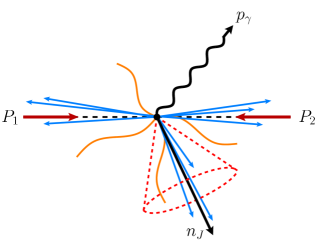
Figure 1: Event topology of direct photon production.

In this section we briefly review some kinematics of direct photon production in a hadron collider and set up our notation. We will follow the conventions in [27], and we summarize the most important kinematic relationships. Once the kinematic variables are defined, we will define our jet definition and the specific observable that we calculate in this paper.

2.1 Hadronic and Partonic Kinematics

We will denote the momenta of the incoming hadrons as $P_{1}^{\mu}$ and $P_{2}^{\mu}$, and the momentum of the photon as $p_{\gamma}^{\mu}$. The observable will be categorized by the properties of the hard photon, namely its transverse momentum $p_{T}$ and rapidity $y$. Formally, the results of this paper will be most accurate when $p_{T}$ is near the machine threshold limit,

$$p_{T}\sim p_{T}^{\rm max}=\frac{E_{\rm CM}}{2\cosh y}\,,$$ (1)

where $E_{\rm CM}=\sqrt{(P_{1}+P_{2})^{2}}$. A majority of events will have photon transverse momenta that are far below the machine threshold limit. However, as we will see, the calculation remains valid for transverse momenta much less than machine threshold due a phenomenon called dynamical threshold enhancement, discussed in Section 3.

A schematic showing the event topology for the collision is given in Figure 1. The hard process involves the collision between two initial state partons, which have momentum $p_{i}^{\mu}=x_{i}P_{i}^{\mu}$ , where the $x_{i}$ is the momentum fraction of the constituent parton and the subscript denotes the hadron from which it came. There are two channels that are relevant at leading order in $\alpha_{s}$, the annihilation channel, $q\bar{q}\to\gamma g$ and the Compton channel, $qg\to\gamma q$. It is convenient to use the variables $w$ and $v$, given by

$$x_{1}=\frac{1}{w}\frac{p_{T}}{E_{\rm CM}v}e^{y}\;,\hskip 28.45274ptx_{2}=\frac{p_{T}}{E_{\rm CM}(1-v)}e^{-y}\;.$$ (2)

The variable $v$ is related to the scattering angle between the photon and the beam, $\theta^{\ast}$, in the partonic center of mass frame through

$$v=\frac{1}{2}(1+\cos\theta^{\ast})\,.$$ (3)

The other variable $w$ characterizes how much the (partonic) event deviates from exact $2\to 2$ kinematics due to additional QCD radiation in the initial or final state. When $w=1$, there is no additional radiation and the partonic final state consists of a photon and either a quark in the case of $qg\to q\gamma$ or a gluon in the case of $q\bar{q}\to g\gamma$.

When discussing the threshold limits, we will discuss the (total) hadronic invariant mass

$$M_{X}^{2}=(P_{1}+P_{2}-p_{\gamma})^{2}\;,$$ (4)

and the (total) partonic invariant mass

$$m_{X}^{2}=(x_{1}P_{1}+x_{2}P_{2}-p_{\gamma})^{2}\;.$$ (5)

These give the invariant mass of all particles in the final state with the photon’s momentum removed from the hadronic or partonic final state, respectively. The hadronic variable $M_{X}$ includes the beam remnant, whereas the partonic version does not have any information about the beam, and therefore $0\leq m_{X}\leq M_{X}$. In terms of the momentum fractions of the partons and the photon transverse momentum and rapidity, the invariant masses are

$$M_{X}^{2}=E_{\rm CM}^{2}-2p_{T}E_{\rm CM}\cosh y=E_{\rm CM}^{2}\left(1-\frac{p_{T}}{p_{T}^{\rm max}}\right)$$ (6)

and

$$m_{X}^{2}=\frac{p_{T}^{2}}{1-v}\frac{1-w}{w}\;.$$ (7)

In the partonic threshold limit, $w\to 1$, there is no phase space volume for the initial or final state radiation, and so the the final state consists of a single scattered parton and a photon. After removing the photon, only a massless parton remains and so the partonic mass vanishes in this limit ($m_{X}\to 0$). The partonic cross section is singular in this limit, and the resulting singularities take the form of $\ln^{2}m_{X}\sim\ln^{2}(1-w)$. In the next section, we will introduce a factorization theorem for the partonic cross section, that will resum the logarithms of $m_{X}$ that appear as $\alpha_{s}^{n}\ln^{m}(1-w)$ in the differential cross section.

2.2 The observable

The observable we consider is the invariant mass of the hardest jet in events with a high $p_{T}$ photon. Rather than use one of the standard jet algorithms to define the jet mass, we use a simple definition in order to make the analytical calculations more tractable. The jet mass used in this paper is defined through the following procedure.

1. Remove the photon from the event record.

2. Cluster the event using the anti-$k_{T}$ jet algorithm.

3. Select the jet with the hardest $p_{T}$, and find its 3-momentum $\mathbf{p}_{J}$. This defines the jet axis as $\hat{n}_{J}=\frac{\mathbf{p}_{J}}{|\mathbf{p}_{J}|}$.

4. Define $m_{R}$ to be the invariant mass of all of the radiation that lies within a cone of half-angle $R$ centered on $\hat{n}_{J}$.

The observable we consider is $\frac{\mathrm{d}\sigma}{\mathrm{d}m_{R}}$, within some range of $p_{T}$ and rapidity for the jet and photon. Our calculation is not sensitive to the difference in $p_{T}$ between the jet and the photon, so we put a cut only on the photon $p_{T}$, integrating inclusively over the $p_{T}$ of the jet. For concreteness our numerical results will have central photons ($y=0$) with a given $p_{T}$, integrated over jet rapidities between $-1$ and $1$.

Although our $R$ differs from a usual collider $R$, which is defined in terms of rapidities and azimuthal angles, the difference is small for central jets that dominate at large $p_{T}$. Our method of calculation, and our factorization theorem, would also work for more standard jet algorithms, such as the $k_{T}$ algorithm. However, most standard algorithms suffer from clustering effects [43, 44, 24, 45, 46] which are not completely understood. Extending the results of this paper to more standard jet algorithms will be explored in future work.

To calculate the jet mass accurately in QCD, one would like the relevant events to come from the hard process we are considering, namely a single photon plus a single parton. However, generically, there can be contributions from events with a hard photon and 2 or 3 jets. The simplest way to ensure single jet kinematics is to use a $p_{T}$ veto on the second hardest jet. This is easy to do experimentally or when using an event generator, but in QCD introducing a new scale makes the theoretical calculation significantly more complicated. In particular, non-global logarithms of the jet mass relative to the veto scale will be introduced. Although these non-global logarithms might be a small effect numerically, an advantage of the threshold resummation is that one does not have to introduce an extra scale. Instead, the scale is implicit in the out-of-jet soft radiation which is integrated over.

By expanding around the threshold limit and demanding large $p_{T}$ for the photon, we can ensure that we are in the photon-plus-single-jet configuration without introducing a new veto scale. When the photon’s $p_{T}$ is on the order of the hard scattering scale, the radiation outside of the hardest jet must be soft, which prevents the formation of a second hard jet. By suitably restricting the photon $p_{T}$, the events will contain a single recoiling jet and we are safely in the regime where the factorization theorem is valid. To put it another way, the fact that dynamical threshold enhancement has been shown to work for the direct photon $p_{T}$ distribution in [27] indicates that the single jet configuration dominates. To be clear, the threshold expansion does not obviate the need to deal with non-global logarithms, as you would with a jet veto, but it does avoid having to deal with an explicit scale.

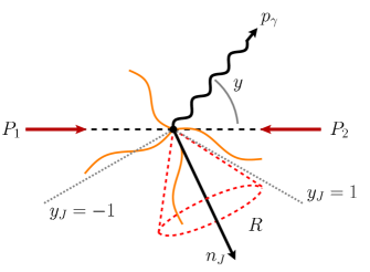
Figure 2: The photon’s momentum and rapidity is denoted by $p_{\gamma}$ and $y$, respectively. The jet cone of half angle $R$, centered around the direction of the jet $n_{J}=(1,\hat{n}_{J})$. The restrictions on the jet rapidity $y_{J}$ is shown by the dashed gray line. Soft radiation inside the jet contributes to $k_{\rm in}=n_{J}\cdot P_{X_{s}^{{\rm in}}}$, whereas the radiation outside contributes to $k_{\rm out}=n_{J}\cdot P_{X_{s}^{{\rm out}}}$

At the partonic threshold limit, where the process only has one parton and a photon in the final state, the $p_{T}$ and $y$ of the photon constrains the scattering angle of the outgoing jet. To see this, consider momentum conservation along the direction of the beam, taken to be the $z$ direction.

$$p_{Jz}=(x_{1}P_{1}+x_{2}P_{2}-p_{\gamma})_{z}$$ (8)

After using the definition of rapidity, $y=\frac{1}{2}\ln\frac{E+p_{z}}{E-p_{z}}$, we can relate the rapidity of the jet $y_{J}$ to the $p_{T}$ and $y$ of the photon and to $x_{1,2}$ via

$$\sinh y_{J}=\frac{E_{\rm CM}}{2p_{T}}(x_{1}-x_{2})-\sinh y\;,$$ (9)

Since $0<x_{1,2}<1$, $y_{J}$ must lie within a range given by

$$-\frac{E_{\rm CM}}{2p_{T}}-\sinh y<\sinh y_{J}<\frac{E_{\rm CM}}{2p_{T}}-\sinh y$$ (10)

In order to perform threshold resummation, we must be careful to keep $y_{J}$ small enough to ensure the jet does not enclose the beams. This restriction is $\sinh y_{J}<\cot R$, and so if we take $|y_{J}|<1$, this implies that $R\lesssim 0.7$.

3 Differential Cross Sections and Factorization Theorem

The differential cross section for the process $N_{1}+N_{2}\to\gamma+X$ can be written in the form

$$\frac{\mathrm{d}^{2}\sigma}{\mathrm{d}p_{T}\mathrm{d}y\mathrm{d}m_{R}^{2}}=\frac{2}{p_{T}}\sum_{ab}\int\!\!\!\!\int_{\mathcal{R}}\mathrm{d}v\mathrm{d}w~{}[x_{1}f_{a/N_{1}}(x_{1},\mu)]~{}[x_{2}f_{b/N_{2}}(x_{2},\mu)]~{}\frac{\mathrm{d}^{2}\hat{\sigma}}{\mathrm{d}w\mathrm{d}v\mathrm{d}m_{R}^{2}}\;,$$ (11)

where $N_{i}$ are the incoming partons, $f_{a/N_{i}}(x_{i},\mu)$ is the probability distribution function for finding parton $a$ in hadron $N_{i}$ with momentum fraction $x_{i}$, and the sum is over the different partonic channels. The region of integration $\mathcal{R}$ in the $w-v$ plane is given by

$$\frac{1+m_{R}^{2}/p_{T}^{2}}{\frac{E_{\rm CM}}{p_{T}}e^{-y}+m_{R}^{2}/p_{T}^{2}}< v <1-\frac{p_{T}}{E_{\rm CM}}e^{-y}$$

$$\frac{e^{y}}{v}\frac{p_{T}}{E_{\rm CM}}< w <\frac{p_{T}^{2}}{p_{T}^{2}+(1-v)m_{R}^{2}}$$

$$\frac{e^{y}}{v(2\sinh y+2\sinh y_{\rm cut}+\frac{1}{1-v}e^{-y})}< w <\frac{e^{y}}{v(2\sinh y-2\sinh y_{\rm cut}+\frac{1}{1-v}e^{-y})}\,.$$ (12)

The first two constraints account for $0\leq x_{i}\leq 1$ and $m_{R}^{2}\leq m_{X}^{2}$ , which is the region enclosed by the red lines in Figure 3; the third constraint comes from a finite rapidity interval for the jet: $-y_{\rm cut}\leq y_{J}\leq y_{\rm cut}$, drawn as the blue lines in Figure 3.

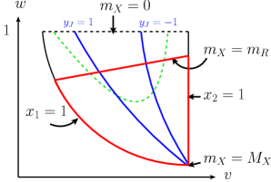
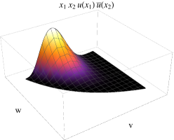
Figure 3: The integration region $\mathcal{R}$ is shown by the red lines. When the jet rapidity is restricted, the region is further constrained to be inside the blue lines, shown here for $y_{\rm cut}=1$. The dashed green line outlines the region that most strongly contributes. This is demonstrated by the right hand plot, which shows the rapid fall off of $x_{1}f_{u/P}(x_{1})x_{2}f_{\bar{u}/P}(x_{2})$.

The expression $\frac{\mathrm{d}^{2}\hat{\sigma}}{\mathrm{d}w\mathrm{d}v\mathrm{d}m_{R}^{2}}$ gives the partonic cross section for $a+b\to\gamma+X$. For a fixed $w$ and $v$, the partonic cross section, at NLO, will diverge logarithmically as $m_{R}\to 0$, and in this regime these logarithms can invalidate an expansion in $\alpha_{s}$.

The reason that the threshold expansion works away from threshold is that the parton distribution functions fall rapidly as the momentum fractions approach unity ($x_{i}\to 1$). In Eq. (15), the partonic differential cross section is weighted by the product of the PDFs. As a representative example, the right side of Figure 3 shows a plot of the product

$$x_{1}f_{u/P}(x_{1},\mu_{f})x_{2}f_{\bar{u}/P}(x_{2},\mu_{f})\;,$$ (13)

which would be necessary for process $u\bar{u}\to\gamma g$. In the plot, we have chosen $E_{\rm CM}=8$ TeV, $p_{T}=2$ TeV, $y=0$, and $\mu_{f}=\sqrt{\hat{s}}=\sqrt{x_{1}x_{2}}E_{\rm CM}$. The plot clearly shows the extremely rapid fall off of the PDFs, and this demonstrates that, for a fixed value of $m_{R}$, the region in $w-v$ space is weighted far more heavily along the line given by $m_{X}=m_{R}$.

The hadronic invariant mass can be written as

$$M_{X}^{2}=\frac{m_{X}^{2}}{x_{2}}+E_{\rm CM}^{2}[(1-x_{1})v+(1-x_{2})(1-v)]\;.$$ (14)

When $M_{X}\to 0$, this forces both $m_{X}\to 0$ and $x_{1,2}\to 1$; however, the fall off the PDFs favor small $m_{X}$ even when $x_{i}$ is not close to 1. Since $m_{R}<m_{X}$, this also means that small $m_{R}$ is favored. The partonic cross section is singular in $m_{R}$, which manifests itself as powers of $\ln m_{R}$, and for small $m_{R}$, these logarithms are large and must be resummed. This enhancement of the singular region for the partonic cross section means that resummation of $m_{R}$ is important, even when we are not near the machine threshold. This effect is known as dynamic threshold enhancement [28, 29, 30].

3.1 Factorization of the partonic cross section

When the jet invariant mass is small compared to the $p_{T}$, the jet is highly collimated and the process can be described within the framework of the Soft-Collinear Effective Theory (SCET) [47, 32, 48, 33]. Rather than give a formal derivation of the factorization formula as in [27], we will focus on how the factorization formula must be modified to become differential in the jet mass.

The partonic differential cross section can be calculated via

$$\frac{\mathrm{d}^{2}\hat{\sigma}}{\mathrm{d}w\mathrm{d}v\mathrm{d}m_{R}^{2}}=w~{}{\tilde{\sigma}}(v)~{}H(p_{T},v,\mu)\int_{0}^{\frac{m_{R}^{2}}{2E_{J}}}\frac{\mathrm{d}k}{2E_{J}}~{}J(m_{R}^{2}-(2E_{J})k,\mu)~{}S(k,\frac{m_{X}^{2}-m_{R}^{2}}{2E_{J}},\mu)\;.$$ (15)

The three functions $H$, $J$ and $S$ are the hard, jet and soft functions, which account for the physics associated with the different scales involved. The quantity ${\tilde{\sigma}}(v)$ is defined through the leading order QCD result via,

$$\frac{\mathrm{d}^{2}\hat{\sigma}}{\mathrm{d}w\mathrm{d}v\mathrm{d}m_{R}^{2}}={\tilde{\sigma}_{ab}}(v)~{}\delta(m_{R}^{2})~{}\delta(m_{X}^{2}-m_{R}^{2})\;,$$ (16)

where the tree level parton cross sections are given by

$$\tilde{\sigma}_{q\bar{q}}(v)=\pi\alpha_{\rm em}e_{q}^{2}\alpha_{s}(\mu)\frac{2C_{F}}{N_{c}}\left(\frac{v^{2}+(1-v)^{2}}{1-v}\right)$$

$$\tilde{\sigma}_{qg}(v)=\pi\alpha_{\rm em}e_{q}^{2}\alpha_{s}(\mu)\frac{1}{N_{c}}(1+(1-v)^{2})\frac{v}{1-v}\;.$$ (17)

The hard function is given by the square of the Wilson coefficients that arise when matching the QCD amplitude onto the effective field theory operators. It describes the short distance physics at an energy scale $\mu_{h}\sim p_{T}$. The jet function comes from integrating energetic modes that are collinear to the jet direction that have virtuality comparable to $m_{R}$. In the threshold limit $m_{R}\ll p_{T}R$, so the collinear radiation is insensitive to the jet boundary. Thus we can use the same inclusive jet function as that in [27]. Finally, once the collinear modes are integrated out, we are left with the soft modes, which are described by soft Wilson lines. The soft function relevant for the jet mass calculation is different from the one used in [27]. As we will see, it depends separately on the radiation inside and outside of the jet, and also on the jet algorithm.

The form of the factorization theorem can be understood from power counting in the threshold region. In the partonic threshold limit, corresponding to the limit $m_{X}\to 0$, radiation is constrained either to be collinear to recoiling parton, which we call $p_{J}^{\mu}$, or to be soft, which we write as $k^{\mu}$. In terms of these momentum regions, the partonic invariant mass takes the form

$$m_{X}^{2}=(p_{J}+k)^{2}=m_{c}^{2}+2k\cdot p_{J}+\cdots$$ (18)

up to terms of order $k^{2}\ll m_{c}^{2}$ where $m_{c}^{2}=p_{J}^{2}$ is the collinear mass, whose distribution is given by the jet function.

The jet invariant mass $m_{R}$ only contains the part of radiation inside the cone. Since all the collinear radiation is in the cone, we have only to split the soft radiation, which we write as $k^{\mu}=k_{\rm in}^{\mu}+k_{\rm out}^{\mu}$, with $k_{\rm in}^{\mu}$ in the cone and $k_{\rm out}^{\mu}$ out of the cone. Then,

$$m_{R}^{2}=(p_{J}+k_{\rm in})^{2}=m_{c}^{2}+2k_{\rm in}\cdot p_{J}\;.$$ (19)

and so

$$m_{X}^{2}=m^{2}_{R}+2k_{\rm out}\cdot p_{J}\;.$$ (20)

Now, the jet momentum $p_{J}^{\mu}$ accounts for radiation that is collinear to recoiling parton, and so it can be written as

$$p_{J}^{\mu}=E_{J}n^{\mu}_{J}+{\rm residual}\;.$$ (21)

where $n_{J}^{\mu}=(1,\hat{n}_{J})$ is a lightlike vector that is directed along the jet direction. The residual momentum gives a power suppressed contribution to the jet mass compared to the leading component, and thus can be dropped. The expressions for $m_{X}$ and $m_{R}$ then become

$$m_{X}^{2} = m^{2}_{R}+2E_{J}(n_{J}\cdot k_{\rm out})$$

$$m_{R}^{2} = m^{2}_{c}+2E_{J}(n_{J}\cdot k_{\rm in})\;.$$ (22)

Therefore, the only component that enters the soft function is $k\equiv n_{J}\cdot k$. These expressions explain the form of the factorization theorem, Eq.(15), which can be written as

$$\frac{\mathrm{d}^{2}\hat{\sigma}}{\mathrm{d}w\mathrm{d}v\mathrm{d}m_{R}^{2}} = w~{}{\tilde{\sigma}}(v)~{}H(p_{T},v,\mu)\int\mathrm{d}k_{\rm in}\mathrm{d}k_{\rm out}\mathrm{d}m^{2}J(m^{2})S(k_{\rm in},k_{\rm out})$$ (23)

$$\qquad\times\delta(m_{R}^{2}-m^{2}-2E_{J}k_{\rm in})\delta(m_{X}^{2}-m_{R}^{2}-2E_{J}k_{\rm out})\;.$$

Furthermore, we see why we need a soft function that depends on the projection of the soft momentum on the jet direction separated into in-cone and out-of cone components, which we denote $k_{\rm in}$ and $k_{\rm out}$.

The precise definition of the soft function we need is, for annihilation channel,

$$S_{q\bar{q}}(k_{\rm in},k_{\rm out})=\frac{1}{C_{F}N_{c}}\sum_{X_{s}}|\langle X_{s}|{\bf T}\Big{[}Y_{1}^{\dagger}Y_{J}t^{a}Y_{J}^{\dagger}Y_{2}(0)\Big{]}|0\rangle|^{2}\delta(n_{J}\cdot P_{X_{s}^{\rm in}}-k_{\rm in})\delta(n_{J}\cdot P_{X_{s}^{\rm out}}-k_{\rm out})\;,$$ (24)

and for Compton channel

$$S_{qg}(k_{\rm in},k_{\rm out})=\frac{1}{C_{F}N_{c}}\sum_{X_{s}}|\langle X_{s}|{\bf T}\Big{[}Y_{1}^{\dagger}Y_{2}t^{a}Y_{2}^{\dagger}Y_{J}(0)\Big{]}|0\rangle|^{2}\delta(n_{J}\cdot P_{X_{s}^{\rm in}}-k_{\rm in})\delta(n_{J}\cdot P_{X_{s}^{\rm out}}-k_{\rm out})\;,$$ (25)

where $P_{X_{s}^{\rm in}}$ and $P_{X_{s}^{\rm out}}$ denote the total momentum of the soft radiation propagating inside and outside the jet, respectively. Also, $Y_{i}$ is a soft Wilson line directed along the $n_{i}=(1,\hat{n}_{i})$ direction:

$$Y^{\dagger}_{i}(x)=P\exp\left(ig\int_{0}^{\infty}ds\ n_{i}\cdot A_{s}(n_{i}s+x)\right)\;,$$ (26)

where $i=1,2,J$ and $P$ denotes path ordering and $A_{s}=A_{s}^{a}T^{a}$ are soft gauge fields in the fundamental representation.

3.2 One-loop soft function

We now calculate the required soft function to order $\alpha_{s}$. The diagrams needed for the calculation are represented in Figure 4.

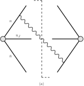
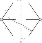
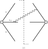
Figure 4: The non-vanishing diagrams that contribute to the one-loop soft function.

The virtual diagrams are not shown as they give a scaleless contribution when using dimensional regularization to regulate both the ultraviolet and infra-red divergences. The non-vanishing diagrams for the $q\bar{q}\rightarrow g\gamma$ channel give

$$S_{q\bar{q}}(k_{\rm in},k_{\rm out},\mu)=\frac{8\pi\alpha_{s}}{(2\pi)^{d-1}}\Big{(}\frac{\mu^{2}e^{\gamma_{E}}}{4\pi}\Big{)}^{\epsilon}\int d^{d}q\ \delta(q^{2})\theta(q_{0})\mathcal{M}(k_{\rm in},k_{\rm out};q)$$

$$\times\Big{[}\Big{(}C_{F}-\frac{1}{2}C_{A}\Big{)}\frac{n_{1}\cdot n_{2}}{(n_{1}\cdot q)(n_{2}\cdot q)}+\frac{1}{2}C_{A}\frac{n_{J}\cdot n_{1}}{(n_{J}\cdot q)(n_{1}\cdot q)}+\frac{1}{2}C_{A}\frac{n_{J}\cdot n_{2}}{(n_{J}\cdot q)(n_{2}\cdot q)}\Big{]}\;,$$ (27)

where $q^{+}=n_{J}\cdot q$, and $q^{-}={\bar{n}}_{J}\cdot q$ with ${\bar{n}}_{J}=(1,-\hat{n}_{J})$, and the measurement function is given by

$$\mathcal{M}(k_{\rm in},k_{\rm out};q) = \Theta\Big{(}\frac{q^{-}-q^{+}}{q^{-}+q^{+}}-\cos R\Big{)}\delta(k_{\rm in}-q^{+})\delta(k_{\rm out})$$ (28)

$$+\Theta\Big{(}\cos R-\frac{q^{-}-q^{+}}{q^{-}+q^{+}}\Big{)}\delta(k_{\rm in})\delta(k_{\rm out}-q^{+})\;.$$

Similarly, for the $qg\rightarrow q\gamma$ channel we have

$$S_{qg}(k_{\rm in},k_{\rm out},\mu)=\frac{8\pi\alpha_{s}}{(2\pi)^{d-1}}\Big{(}\frac{\mu^{2}e^{\gamma_{E}}}{4\pi}\Big{)}^{\epsilon}\int d^{d}q\ \delta(q^{2})\theta(q_{0})\mathcal{M}(k_{\rm in},k_{\rm out};q)$$

$$\times\Big{[}\frac{1}{2}C_{A}\frac{n_{1}\cdot n_{2}}{(n_{1}\cdot q)(n_{2}\cdot q)}+\Big{(}C_{F}-\frac{1}{2}C_{A}\Big{)}\frac{n_{J}\cdot n_{1}}{(n_{J}\cdot q)(n_{1}\cdot q)}+\frac{1}{2}C_{A}\frac{n_{J}\cdot n_{2}}{(n_{J}\cdot q)(n_{2}\cdot q)}\Big{]}.$$ (29)

The soft function will depend on the angle $R$ and the rapidity of the jet $y_{J}$. For convenience we define

$$r=\tan\frac{R}{2}\hskip 28.45274pt\beta=\exp(-y_{J})$$ (30)

With these definitions, the soft functions associated with the two channels at order $\alpha_{s}$ are

$$S_{q\bar{q}}(k_{\rm in},k_{\rm out},\mu) = \delta(k_{\rm in})\delta(k_{\rm out})+2\Big{(}\frac{\alpha_{s}}{4\pi}\Big{)}\Big{\{}\delta(k_{\rm in})\delta(k_{\rm out})\Big{(}C_{F}-\frac{1}{2}C_{A}\Big{)}\Big{[}\ln^{2}\frac{(1+\beta^{2})^{2}}{\beta^{2}}-\frac{\pi^{2}}{6}\Big{]}$$ (31)

$$+ 2\frac{\delta(k_{\rm out})}{k_{\rm in}}\Big{[}-2C_{A}\ln\Big{(}\frac{k_{\rm in}}{\mu}\frac{1+\beta^{2}}{\beta}\Big{)}+c_{q\bar{q}}\Big{]}$$

$$+ 2\frac{\delta(k_{\rm in})}{k_{\rm out}}\Big{[}4C_{F}\ln\Big{(}\frac{k_{\rm out}}{\mu}\frac{1+\beta^{2}}{\beta}\Big{)}-c_{q\bar{q}}\Big{]}\Big{\}}\;,$$

and

$$S_{qg}(k_{\rm in},k_{\rm out},\mu) = \delta(k_{\rm in})\delta(k_{\rm out})+2\Big{(}\frac{\alpha_{s}}{4\pi}\Big{)}\Big{\{}\delta(k_{\rm in})\delta(k_{\rm out})\Big{(}\frac{1}{2}C_{A}\Big{)}\Big{[}\ln^{2}\frac{(1+\beta^{2})^{2}}{\beta^{2}}-\frac{\pi^{2}}{6}\Big{]}$$ (32)

$$+ 2\frac{\delta(k_{\rm out})}{k_{\rm in}}\Big{[}-2C_{F}\ln\Big{(}\frac{k_{\rm in}}{\mu}\frac{1+\beta^{2}}{\beta}\Big{)}+c_{qg}\Big{]}$$

$$+ 2\frac{\delta(k_{\rm in})}{k_{\rm out}}\Big{[}(2C_{F}+2C_{A})\ln\Big{(}\frac{k_{\rm out}}{\mu}\frac{1+\beta^{2}}{\beta}\Big{)}-c_{qg}\Big{]}\Big{\}}\;,$$

where

$$c_{q\bar{q}} = -C_{F}\ln\left[\frac{(\beta^{2}-r^{2})(1-r^{2}\beta^{2})}{\beta^{2}r^{4}}\right]-C_{A}\ln\frac{\beta^{2}}{(1+\beta^{2})^{2}}+(2C_{F}-C_{A})\ln\frac{1+r^{2}}{r^{2}}$$

$$c_{qg} = \Big{[}-C_{F}\ln\frac{\beta^{2}-r^{2}}{r^{2}\beta^{2}}-C_{A}\ln\frac{1-r^{2}\beta^{2}}{r^{2}\beta^{2}}\Big{]}-C_{F}\ln\frac{\beta^{2}}{(1+\beta^{2})^{2}}+C_{A}\ln\frac{1+r^{2}}{r^{2}}\;.$$ (33)

The logarithmic divergences involving $r$ and $\beta$ arise when the jet cone encloses the collinear radiations from one of the incoming beams.

Since the factorization theorem contains convolutions between the jet and soft functions, it is easier to perform the calculation in Laplace space. The Laplace transformed soft function is defined as

$${\tilde{s}}(\kappa_{\rm in},\kappa_{\rm out},\mu) = \int_{0}^{\infty}dk_{\rm in}\int_{0}^{\infty}dk_{\rm out}\exp\Big{(}-\frac{k_{\rm in}}{\kappa_{\rm in}e^{\gamma_{E}}}\Big{)}\exp\Big{(}-\frac{k_{\rm out}}{\kappa_{\rm out}e^{\gamma_{E}}}\Big{)}S(k_{\rm in},k_{\rm out},\mu)\;.$$

Our result is then

$${\tilde{s}}_{q\bar{q}}(L_{1},L_{2},\mu) = 1+\Big{(}\frac{\alpha_{s}}{4\pi}\Big{)}\Big{[}4(2C_{F}L_{2}^{2}-C_{A}L_{1}^{2})+4(L_{1}-L_{2})c_{q\bar{q}}+\Big{(}C_{F}-\frac{1}{2}C_{A}\Big{)}\pi^{2}\Big{]}$$

$${\tilde{s}}_{qg}(L_{1},L_{2},\mu) = 1+\Big{(}\frac{\alpha_{s}}{4\pi}\Big{)}\Big{[}4((C_{F}+C_{A})L_{2}^{2}-C_{F}L_{1}^{2})+4(L_{1}-L_{2})c_{qg}+\Big{(}\frac{1}{2}C_{A}\Big{)}\pi^{2}\Big{]}\;,$$

where $L_{1}=\ln\Big{(}\frac{1+\beta^{2}}{\beta}\frac{\kappa_{\rm in}}{\mu}\Big{)}$ and $L_{2}=\ln\Big{(}\frac{1+\beta^{2}}{\beta}\frac{\kappa_{\rm out}}{\mu}\Big{)}$.

The renormalization group equations satisfied by the soft function in the two channels are

$$\frac{d\tilde{s}_{q\bar{q}}}{d\ln\mu} = \Big{[}2C_{A}\gamma_{\rm cusp}\ln\Big{(}\frac{1+\beta^{2}}{\beta}\frac{\kappa_{\rm in}}{\mu}\Big{)}-4C_{F}\gamma_{\rm cusp}\ln\Big{(}\frac{1+\beta^{2}}{\beta}\frac{\kappa_{\rm out}}{\mu}\Big{)}-2\gamma^{S_{q{\bar{q}}}}\Big{]}\tilde{s}_{q\bar{q}}$$

$$\frac{d\tilde{s}_{qg}}{d\ln\mu} = \Big{[}2C_{F}\gamma_{\rm cusp}\ln\Big{(}\frac{1+\beta^{2}}{\beta}\frac{\kappa_{\rm in}}{\mu}\Big{)}-2(C_{F}+C_{A})\gamma_{\rm cusp}\ln\Big{(}\frac{1+\beta^{2}}{\beta}\frac{\kappa_{\rm out}}{\mu}\Big{)}-2\gamma^{S_{qg}}\Big{]}\tilde{s}_{qg}\;.$$

where the expressions for $\gamma_{\rm cusp}$, $\gamma^{S_{q\bar{q}}}$, $\gamma^{S_{qg}}$ are given to order $\alpha_{s}^{2}$ in [27] and are known to order $\alpha_{s}^{3}$.

To check that the factorization theorem in Eq. (15) is correct, we have confirmed that the $\mu$-dependence of the hard, jet, soft functions and PDFs near $x=1$ cancel when combined. We also compare the singular part of the full QCD distribution at high $p_{T}$ which we compute using the numerical package mcfm to the distribution produced by combining the hard, jet and soft functions at fixed order. This is shown in Figure 8.

Although the factorization theorem is correct, it does not automatically guarantee that we can resum all of the logarithms of $m_{R}$. Recall that the soft function in the factorization theorem in [27] was fully inclusive and had dependence only on the projection of the soft momentum in the jet direction. For the inclusive photon $p_{T}$ spectrum, such a one-scale soft function is natural, since the observable only depends on a single scale, $p_{T}$. In contrast, the soft functions given in Eqs. (24) and (25) depend on two physical scales $k_{\rm in},k_{\rm out}$ as well as on the renormalization scale $\mu$. With multiple soft scales, there may not be a natural choice for $\mu$, and therefore the renormalization group evolution may not resum all of the large logarithms. Indeed, in a analogous jet mass calculation for an $e^{+}e^{-}$ collider, it was demonstrated first numerically in [21] and then analytically in [25] that the singularity structure of QCD was not completely reproduced by expanding the resummed result for jet thrust. One expects the same difficulty here.

The problem is that our soft function anomalous dimension does not depend on jet size $R$. This is simply because the hard and jet functions as well as the PDFs are the same as in the inclusive case and do not have a jet size dependence. However, there are large logarithms in full QCD that could only be predicted from an $R$-dependent anomalous dimension. To make this point more concrete, consider the singular part of the cross section calculated to ${\mathcal{O}}(\alpha_{s})$ using SCET in the annihilation channel:

$$\frac{d\hat{\sigma}_{q\bar{q}}}{\mathrm{d}w\mathrm{d}v\mathrm{d}m_{R}^{2}}=w{\tilde{\sigma}_{q\bar{q}}}(v)\delta(m_{X}^{2}-m_{R}^{2})\frac{\alpha_{s}(\mu)}{4\pi}\frac{-2C_{A}\Gamma_{0}\ln\frac{m_{R}^{2}}{p_{T}\mu}+{c_{q\bar{q}}(r,\beta)}\Gamma_{0}+\Gamma^{J_{g}}_{0}\ln\frac{m_{R}^{2}}{\mu^{2}}+\gamma^{J_{g}}_{0}}{m_{R}^{2}}$$ (37)

Since SCET contains all of the singular contributions from full QCD, this will agree with the full one-loop QCD result expanded at small $m_{R}$. However, we should also be able to predict these $\frac{1}{m_{R}^{2}}$ terms only using the anomalous dimensions, since they should be part of the resummation at NLL level. Since the coefficient of $\frac{1}{m_{R}^{2}}$ depends on $r=\tan R/2$ through the ${c_{q\bar{q}}(r,\beta)}$ term, this is impossible for $R$-independent anomalous dimensions. Thus, without further insight, resummation in SCET will undoubtedly miss these logarithmic corrections.

4 Refactorization of the Soft Function

The soft function depends on the two scales $k_{\rm in}$ and $k_{\rm out}$. By explicit calculation we found it has logarithmic dependence on both of the scales divided by $\mu$ already at one loop. Since there is not a single scale associated with the soft function, we should not expect that a single choice of $\mu$ will give the soft function a controlled perturbative expansion. In addition, at two loops, one generically expects a complicated dependence on $k_{\rm in}/k_{\rm out}$ in the soft function, as was found in [49, 25], representative of the non-global structure. The problem, from an effective theory point of view, is that there are two modes with different characteristic scaling described by the same object. Ideally, we could factorize the soft function into separate objects which depend only on $k_{\rm in}/\mu$ and $k_{\rm out}/\mu$. However, it does not appear that the soft function exactly factorizes in that way.

In the absence of a full refactorization, we will proceed in a conservative fashion following methods of traditional resummation [50, 51, 52, 53, 54, 55]. To that end, we can at least isolate part of the soft function whose scaling we already know, namely the part associated with radiation that goes entirely into the jet, which will at least contain all of the soft-collinear divergences. To do so, we will define an auxiliary soft function that only depends on $k_{\rm in}$, reminiscent of eikonal jet functions in [50]. There are many ways to do this. A simple choice is to define the auxiliary soft function the same way we define the 2-scale soft function, but inclusive over the out-of-jet radiation. That is, we take

$$\hat{S}_{q\bar{q}}(k_{\rm in})=\frac{1}{C_{F}N_{c}}\sum_{X_{s}}|\langle X_{s}|{\bf T}\Big{[}Y_{1}^{\dagger}Y_{J}t^{a}Y_{J}^{\dagger}Y_{2}(0)\Big{]}|0\rangle|^{2}\delta(k_{\rm in}-n_{J}\cdot P_{X_{s}^{\rm in}})\;,$$ (38)

for the annihilation channel, and similarly for the Compton channel. We call this a regional soft function. The regional soft function was deliberately chosen to have the same color structure as the original soft function.

At one-loop the regional soft function is given by Eqs. (3.2) and (3.2) with the measurement function replaced by

$$\mathcal{M}(k_{\rm in};q) = \Theta\Big{(}\frac{q^{-}-q^{+}}{q^{-}+q^{+}}-\cos R\Big{)}\delta(k_{\rm in}-q^{+})\;.$$ (39)

At order $\alpha_{s}$, we find

$$\hat{S}_{q\bar{q}}(k_{\rm in},\mu) = \delta(k_{\rm in})+2\Big{(}\frac{\alpha_{s}}{4\pi}\Big{)}\Big{\{}\delta(k_{\rm in})\Big{(}-\frac{1}{2}C_{A}\Big{)}\Big{[}\ln^{2}\frac{(1+\beta^{2})^{2}}{\beta^{2}}-\frac{\pi^{2}}{6}\Big{]}$$

$$+ 2\frac{1}{k_{\rm in}}\Big{[}-2C_{A}\ln\Big{(}\frac{k_{\rm in}}{\mu}\frac{1+\beta^{2}}{\beta}\Big{)}+c_{q\bar{q}}\Big{]}\;,$$

$$\hat{S}_{qg}(k_{\rm in},\mu) = \delta(k_{\rm in})+2\Big{(}\frac{\alpha_{s}}{4\pi}\Big{)}\Big{\{}\delta(k_{\rm in})\Big{(}-\frac{1}{2}C_{F}\Big{)}\Big{[}\ln^{2}\frac{(1+\beta^{2})^{2}}{\beta^{2}}-\frac{\pi^{2}}{6}\Big{]}$$ (40)

$$+ 2\frac{1}{k_{\rm in}}\Big{[}-2C_{F}\ln\Big{(}\frac{k_{\rm in}}{\mu}\frac{1+\beta^{2}}{\beta}\Big{)}+c_{qg}\Big{]}\;,$$

where $c_{q\bar{q}}$ and $c_{qg}$ are given in Eq. (3.2). The anomalous dimensions at order $\alpha_{s}$, in Laplace space, are

$$\frac{d}{d\ln\mu}\tilde{s}_{q\bar{q}}(\kappa_{\rm in},\mu) = \frac{\alpha_{s}}{4\pi}\Big{[}2C_{A}\Gamma_{0}\ln\left(\frac{1+\beta^{2}}{\beta}\frac{\kappa_{\rm in}}{\mu}\right)-4c_{q\bar{q}}(r,\beta)\Big{]}\tilde{s}_{q\bar{q}}(\kappa_{\rm in},\mu)$$

$$\frac{d}{d\ln\mu}\tilde{s}_{qg}(\kappa_{\rm in},\mu) = \frac{\alpha_{s}}{4\pi}\Big{[}2C_{F}\Gamma_{0}\ln\left(\frac{1+\beta^{2}}{\beta}\frac{\kappa_{\rm in}}{\mu}\right)-4c_{qg}(r,\beta)\Big{]}\tilde{s}_{qg}(\kappa_{\rm in},\mu)\;,$$ (41)

The dependence of the soft function on $k_{\rm out}$ is still encoded in the full soft function, so we define the residual soft function to be what remains after dividing the full soft function by the regional soft function.

$$S_{r}(k_{\rm in},k_{\rm out},\mu)=\frac{S(k_{\rm in},k_{\rm out},\mu)}{\hat{S}(k_{\rm in},\mu)}$$ (42)

At order $\alpha_{s}$, the contribution from radiation going inside the jet is identical between the full soft function and the regional soft function. When the radiation goes outside of the jet, it contributes to $k_{\rm out}$ in the full contribution, however its contribution to the regional soft function vanishes since the integral is scaleless. Thus the residual soft function at order $\alpha_{s}$ only has $k_{\rm out}$ dependence:

$${S_{r}}_{q\bar{q}}(k_{\rm in},k_{\rm out},\mu) = \delta(k_{\rm out})+2\Big{(}\frac{\alpha_{s}}{4\pi}\Big{)}\Big{\{}\delta(k_{\rm out})\Big{(}C_{F}\Big{)}\Big{[}\ln^{2}\frac{(1+\beta^{2})^{2}}{\beta^{2}}-\frac{\pi^{2}}{6}\Big{]}$$

$$+ 2\frac{1}{k_{\rm out}}\Big{[}4C_{F}\ln\Big{(}\frac{k_{\rm out}}{\mu}\frac{1+\beta^{2}}{\beta}\Big{)}-c_{q\bar{q}}\Big{]}\Big{\}}$$

$${S_{r}}_{qg}(k_{\rm in},k_{\rm out},\mu) = \delta(k_{\rm out})+2\Big{(}\frac{\alpha_{s}}{4\pi}\Big{)}\Big{\{}\delta(k_{\rm out})\Big{(}\frac{1}{2}C_{F}+\frac{1}{2}C_{A}\Big{)}\Big{[}\ln^{2}\frac{(1+\beta^{2})^{2}}{\beta^{2}}-\frac{\pi^{2}}{6}\Big{]}$$ (43)

$$+ +2\frac{1}{k_{\rm out}}\Big{[}(2C_{F}+2C_{A})\ln\Big{(}\frac{k_{\rm out}}{\mu}\frac{1+\beta^{2}}{\beta}\Big{)}-c_{qg}\Big{]}\Big{\}}\;.$$

Thus, the one-loop anomalous dimensions of the residual soft function depends only on the Laplace conjugate variable for $k_{\rm out}$, $\kappa_{\rm out}$:

$$\frac{d}{d\ln\mu}\tilde{s}_{rq\bar{q}}(\kappa_{\rm out},\mu) = \frac{\alpha_{s}}{4\pi}\Big{[}-4C_{F}\Gamma_{0}\ln\left(\frac{1+\beta^{2}}{\beta}\frac{\kappa_{\rm out}}{\mu}\right)+4c_{q\bar{q}}(r,\beta)\Big{]}\tilde{s}_{rq\bar{q}}(\kappa_{\rm out},\mu)$$

$$\frac{d}{d\ln\mu}\tilde{s}_{rqg}(\kappa_{\rm out},\mu) = \frac{\alpha_{s}}{4\pi}\Big{[}-2(C_{F}+C_{A})\Gamma_{0}\ln\left(\frac{1+\beta^{2}}{\beta}\frac{\kappa_{\rm out}}{\mu}\right)+4c_{qg}(r,\beta)\Big{]}\tilde{s}_{rqg}(\kappa_{\rm out},\mu)\;,$$

Combining these results, we see that we have actually factorized the soft function at one-loop, since the regional and residual soft functions each depend on only one scale. At two-loops and higher, the regional soft function will still only depend on $k_{\rm in}$, however the residual soft function will have both $k_{\rm in}$ and $k_{\rm out}$ dependence. Thus, at least there should be a natural scale which minimizes the large logarithms in $\hat{S}(k_{\rm in},\mu)$. In particular, this scale should correspond to the “see-saw” scale $\mu_{s}=\mu_{j}^{2}/\mu_{h}$ for the soft radiation associated with a particular collinear direction [56]. Such a scale assignment is implicit in much of the work on traditional resummation, and here we have made it explicit using SCET.

For this refactorization to make any difference, we have to allow the residual soft function scale to be different from the scale for the regional soft function. So we write

$$S(k_{\rm in},k_{\rm out},\mu)=\hat{\Pi}(\mu,\mu_{\rm in})\hat{S}(k_{\rm in},\mu_{\rm in})\Pi_{r}(\mu,\mu_{\rm out})S_{r}(k_{\rm in},k_{\rm out},\mu_{\rm out})$$ (45)

where the evolution kernels $\hat{\Pi}(\mu,\mu_{\rm in})$ and $\Pi_{r}(\mu,\mu_{\rm out})$ evolve their respective soft functions from $\mu$ to separate scales. In Section 6, we investigate how choosing two soft scales affects the jet mass distribution by comparing the calculation with and without such a scale separation (see Figure 9).

Unfortunately, since the residual soft function will depend on both $k_{\rm in}$ and $k_{\rm out}$ beyond one-loop, our refactorization is only approximate. At two-loops, the $k_{\rm in}/k_{\rm out}$ dependence of the residual soft function is due to non-global structure. When the scales are widely separated, $k_{\rm in}\ll k_{\rm out}$ or vice verse, the non-global structure takes the form of a logarithm of the ratio of these scales. There have been many studies of non-global logarithms (NGLs) [36, 37, 38, 39, 19, 49, 57, 24, 25]. We will not attempt to calculate the non-global structure for this observable, which would require a two-loop calculation, instead we will estimate their effects and discuss their phenomenological significance in Section 7.

4.1 Comparing with pQCD result

Calculating the jet mass distribution at hadron collider has been done by using traditional pQCD resummation technique [23, 26, 58]. It’s interesting to compare the pQCD results and the SCET results obtained in this paper. In Refs. [23, 26], the jet mass distribution is described by a process independent quark or gluon jet function, depending on the partonic origin of the jet. These pQCD jet functions are calculated to $\mathcal{O}(\alpha_{s})$ explicitly, and resumed to all orders at NLL level by solving an evolution equation in Mellin space. In their approach, both the hard-collinear mode and soft mode contribute to the jet function, in contrast to the SCET approach, where jet function is defined with zero-bin subtraction [59]. Furthermore, the jet function defined in Refs. [23, 26] is independent of underlying partonic process, and the corresponding jet mass distribution misses the contribution from soft large angle radiation between different colored partons. Therefore a simple connection between their jet function and our SCET results can not be made.

To make progress comparing the different formalisms, it is helpful to consider the $R\to 0$ limit. In this limit, a process independent combination of jet and soft function can be defined in SCET. For example, for the annihilation channel, we have

$$J_{g}^{SCET}(m^{2}_{R},\mu)=\lim_{R\to 0}\int dp^{2}dk_{\rm in}\,J_{g}(p^{2},\mu)S_{q\bar{q}}(k_{\rm in},\mu)\delta(m^{2}_{R}-p^{2}-2E_{J}k_{\rm in}),$$ (46)

and similarly for the Compton channel. The fact that in the $R\to 0$ limit $S_{q\bar{q}}$ depends only on the parton that initiates the jet can be seen explicitly by taking the limit in Eq. (4). In this limit, only the terms proportional to $\ln r$ survive, each of which is proportional the jet’s Casimir – $C_{F}$ for quark jet and $C_{A}$ for a gluon jet. Alternatively, it can be understood by the rescaling argument from [25]. To be specific, by rescaling $R$ to $\pi/2$, the cone of the $\hat{n}_{J}$-jet becomes a hemisphere. At the same time, all other Wilson lines, except the one along the jet direction, are forced to point in the direction of $-\hat{n}_{J}$. Therefore, a soft dipole contribution from partons $i$ and $J$, where $i$ denotes an initial state parton, is identical to the hemisphere soft function [25], with the color factor replaced by $-T_{i}\cdot T_{J}$ in the color generator notation [60], while dipoles contributes from two initial state partons $i$ and $j$ vanish. Since $(-T_{1}\cdot T_{J}-T_{2}\cdot T_{J})=T^{2}_{J}$, summation over different soft dipole gives a result which depends only on the jet direction and its color content. This explains why the jet function constructed in Eq. (46) depends only on the parton that initiates the jet. Indeed, at $\mathcal{O}(\alpha_{s})$, for quark and gluon jet, we have

$$J^{SCET}_{q}(m^{2}_{R},\mu) = \frac{\alpha_{s}(\mu)C_{F}}{\pi m^{2}_{R}}\left(\log\frac{4E^{2}_{J}\sin^{2}\frac{R}{2}}{p^{2}_{T}}-\frac{3}{4}\right),$$

$$J^{SCET}_{g}(m^{2}_{R},\mu) = \frac{\alpha_{s}(\mu)}{\pi m^{2}_{R}}\left(C_{A}\log\frac{4E^{2}_{J}\sin^{2}\frac{R}{2}}{p^{2}_{T}}-\frac{11}{12}C_{A}+\frac{1}{3}n_{f}T_{F}\right),$$ (47)

respectively, where $n_{f}$ is the number of light flavor and $T_{F}=1/2$ in QCD. Eq. (47) agrees with the corresponding $\mathcal{O}(\alpha_{s})$ jet function in Eqs. (A3) and (A4) of Refs. [26], after power expanding in jet mass, except the term proportional to $n_{f}T_{F}$, which is missing there. From the discussion above, we see that the results presented in Refs. [23, 26] are not complete at NLL level, missing the contribution from large angle soft cross talk, as well as the term proportional to $n_{f}T_{F}$ in the gluon jet function. These extra global NLL contributions are taken into account in a more recent work [58], which also includes a numerical exponentiation of part of the non-global structure.

5 Scale Choices

While the resummed result is formally independent of the scales $\mu_{h}$, $\mu_{j}$, $\mu_{{\rm in}}$ and $\mu_{{\rm out}}$ as well as the factorization scale we call $\mu$, there is residual higher-order dependence on these scales if the perturbative expansions of the hard, jet and soft functions are truncated at a finite order. To get a well behaved expansion with minimum hard, jet and soft scale dependence, we want to evaluate each contribution at its natural scale where each function does not involve large perturbative logarithms. We evolve the hard, jet and soft functions from their natural scales to the factorization scale $\mu$ as shown in Figure 5.

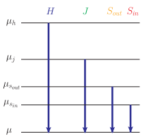
Figure 5: The renormalization group evolution of the hard, jet and soft functions, as shown schematically. Each function is calculated at fixed order at its natural scale, and they are evolved to a common scale $\mu$. Two scales emerge in the soft sector which results in the refactorization of the soft function.

In the resummed distribution, the following ratios of scales appear

$$\frac{p_{T}^{2}}{\mu_{h}^{2}}\;,\qquad\frac{m_{R}^{2}}{\mu_{j}^{2}}\;,\qquad\frac{\mu_{j}^{2}}{p_{T}\mu_{{\rm in}}}\;,\qquad\frac{m_{X}^{2}-m_{R}^{2}}{p_{T}\mu_{{\rm out}}}\;.$$ (48)

Unlike the fully inclusive case studied in [27], it would be impossible to minimize logarithms of these ratios with only 3 scales $\mu_{h}$, $\mu_{j}$ and $\mu_{s}=\mu_{{\rm in}}=\mu_{{\rm out}}$. Instead, we will allow $\mu_{{\rm in}}$ and $\mu_{{\rm out}}$ to be independent, as explained in Section 4. When we choose a single soft scale, the resummed SCET distribution is hopelessly different from the pythia output – this is shown in Figure 9.

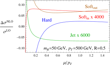
Figure 6: The NLO corrections of the hard, jet and soft functions to the jet mass distribution as a function of the renormalization scale for $m_{R}=50$ GeV and $p_{T}=500$ GeV . The natural scale of each mode is indicated by the of the extremum of the appropriate curve. The hard and $\rm soft_{\rm out}$ scales do not depend on the mass of the jet; they are determined by varying the scales with the NLO delta function contributions. The jet and $\rm soft_{\rm in}$ scales are determined by varying the scales with the NLO jet mass distribution. The jet and $\rm soft_{\rm in}$ curves are scaled up to plot with the ones for the hard and $\rm soft_{\rm out}$.

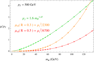
Figure 7: The jet and $\rm soft_{\rm in}$ scales as a function of $m_{R}$ for $p_{T}=500$ GeV with two different cone sizes. Dots are extrema and curves are our fits. Note that $\mu_{{\rm in}}$ is cone size dependent and increases when the cone gets smaller. However, $\mu_{j}^{2}/\mu_{{\rm in}}$ is $m_{R}$ independent, which is a manifestation of the factorization theorem. The numerically determined jet and $\rm soft_{\rm in}$ scales fit nicely with power law curves ($m_{R}$ in GeV): $\mu_{j}=1.6~{}m_{R}^{1.47}$, $\mu_{{\rm in}}(R=0.3)=\mu_{j}^{2}/2300$, $\mu_{{\rm in}}(R=0.5)=\mu_{j}^{2}/6700$, and they are considerably higher than the naive choices of $\mu_{j}=m_{R}$ and $\mu_{{\rm in}}=m_{R}^{2}/p_{T}$.

The naive scale choices are

$$\mu_{h}=p_{T}\;,\qquad\mu_{j}=m_{R}\;,\qquad\mu_{{\rm in}}=\frac{m_{R}^{2}}{p_{T}}\;,\qquad\mu_{{\rm out}}=\frac{m_{X}^{2}-m_{R}^{2}}{p_{T}}\;,$$ (49)

These would eliminate the large logarithms at each energy scale at the partonic level. However, when the partonic cross section is integrated against the PDFs, $\mu_{{\rm out}}$ will get arbitrarily close to zero and hit the Landau pole singularity of the running coupling. The problem is that the natural $\mu_{\rm out}$ scale choice depends on an unphysical quantity, namely $m_{X}^{2}-m_{R}^{2}$. We can avoid the Landau pole and minimize the effects of the large logarithms by instead choosing the scales numerically to depend only on observables [30]. In fact, it is not necessary to eliminate the logarithms in the unphysical, partonic cross section, but rather we want to eliminate the large logarithm in the physical, hadronic cross section.

To determine the natural RG scales, we follow the approach used in [30, 27, 40, 41]. We include separately the NLO corrections for the hard, jet or soft functions and vary the relevant scale to find out which scale minimizes the variation of the NLO distribution. For example, Figure 6 shows these NLO corrections for the 8 TeV LHC with a $p_{T}=500$ GeV photon and $m_{R}=50$ GeV. The extrema of these curves indicate a natural scale for each mode, and one can see that there is a natural hierarchy of the various matching scales. The jet and $\rm soft_{\rm in}$ scales are jet mass dependent, whereas the hard and $\rm soft_{\rm out}$ scales are jet mass independent (their NLO contributions have no dependence on $m_{R}$). We fit the jet mass dependence by power law curves, examples of which are shown in Figure 7 for different jet sizes. For example, with $R=0.5$, the scale choice we extract are

$$\mu_{h}=p_{T};,\qquad\mu_{j}=1.6~{}m_{R}^{1.47}\;,\qquad\mu_{{\rm in}}=\frac{\mu_{j}^{2}}{6700}\;,\qquad\mu_{{\rm out}}=280~{}{\rm GeV}.$$ (50)

We choose the factorization scale to match the hard scale, $\mu=\mu_{h}$ (a high factorization scale is not natural in SCET, however it corresponds most closely to the scales where the PDFs have been fit). The renormalization group is then used to run between these scales to producing the resummed jet mass distribution. For simplicity, we extract these curves at fixed $p_{T}$ and $y$ for the photon, although one could easily repeat this exercise integrated over some window of photon kinematics.

6 Results

To test our predictions, we compare our results to the output from pythia 8 [42] for the LHC at $E_{\rm CM}=8$ TeV. We use the MSTW 2008 NLO PDFs [61] both for event generation and theory calculation. The event generation is made with the hadronization turned off, except for one curve on the right hand side of Figure 9, where you can see that it affects the peak region. For the rest of plots, we keep the initial state and final state radiation, but we turn off hadronization, underlying event and multiple interactions. These additional effects are important, but we postpone their consideration to future work. The specific observable we use is outlined in Section 2.2, and we test several values of $R$. The jet mass distribution is calculated and compared to pythia in a small window of the photon transverse momentum and rapidity $(\Delta p_{T},\Delta y)=(10~{}{\rm GeV},0.1)$, centered around $p_{T}=500$ or $2000$ GeV and $y=0$, for various sizes of $R$.

Since SCET contains all the physics in the small $m_{R}$ regime, it should reproduce the singular structure of full QCD at leading order. We check this by comparing the fixed order expansion of SCET to the exact leading order distribution, using MCFM [62], in the far singular region. The result is shown in Figure 8, which shows very good agreement down to very small $m_{R}$. We also compare MCFM with pythia, and there is no region of $m_{R}$ in which the QCD NLO calculation agrees, which suggests the necessity of resummation.

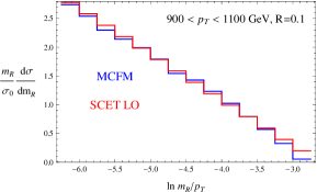
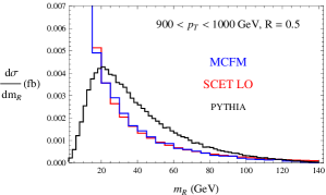
Figure 8: The left panel shows a comparison of the leading order jet mass distirbution calculated with MCFM and the prediction from expanding the resummed result to leading order (SCET LO). This demonstrates that SCET reproduces the singularities of QCD at leading order. The right panel compares MCFM and SCET to pythia, with obvious disagreement, indicating the importance of resummation.

We calculate the jet mass distribution at full next-to-leading log (NLL) precision, which involves the two-loop cusp anomalous dimension and the one loop anomalous dimensions of the hard, jet and soft functions. In fact, all ingredients are known for NNLL resummation, except for the contribution of non-global logarithms. We estimate the effect of these missing NGLs in Section 7. We denote the partial next-to-next-to-leading log resummed result as $\rm NNLL_{p}$, which has the three loop cusp anomalous dimension and the two-loop anomalous dimensions of the hard, jet and full soft functions. We have only included those parts of the $\mathcal{O}(\alpha_{s}^{2})$ soft anomalous dimension that can be extracted from the RG invariance of the cross section, which does not include the angle-dependent pieces.

Figure 9 shows the jet mass distributions for the $p_{T}=500$ GeV events at different orders of precision.

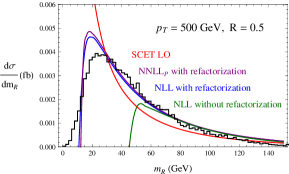
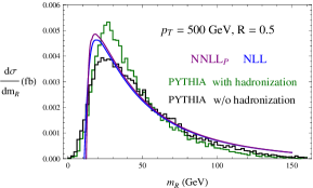
Figure 9: Comparison of the jet mass distributions with different orders of precision (curves) for $p_{T}=500$ GeV and $R=0.5$ to pythia (histograms). The right plot shows the effects of hadronization in pythia as compared to resummed distributions.

For this $p_{T}$, we compute the jet mass distribution with a maximum cone size of $R=0.5$ to avoid the jet being contaminated by the beam. We normalize the SCET distributions with the NLO QCD cross section as determined by pythia 8, scaled by the QCD NLO $K$-factor for the cross-section with the jet rapidity restriction ($K\sim 0.8$ for a 500 GeV photon), which we compute with our own code. We do not match to the exact LO QCD calculation which would account the power corrections in the tail. In the peak region, where most of the events lie, these power corrections are small. The scale uncertainties for the resummed result include variation of the factorization scale $\mu_{f}=\mu$, the hard scale $\mu_{h}$, the jet scale $\mu_{j}$, and the soft scales $\mu_{{\rm in}}$ and $\mu_{{\rm out}}$, Figure 10 shows the uncertainty bands for separate variation of the scales between $\frac{1}{2}\mu_{i}<\mu<2\mu_{i}$ for $i=f,h,j,s_{\rm in},s_{\rm out}$, for $p_{T}=500$ GeV and $R=0.5$ jets. Additional comparisons for $p_{T}=2$ TeV and $R=0.4$ are shown in Figures 11 and 12. The higher the transverse momentum of the photon, the closer to threshold, so we expect that threshold resummation will be more effective in this case.

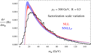
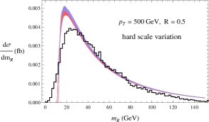
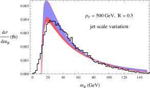
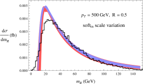
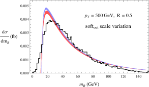
Figure 10: Scale uncertainties for $p_{T}=500$ GeV and $R=0.5$. The red bands are NLL and the blue bands are $\rm NNLL_{p}$. The pythia result is the histogram shown in black.

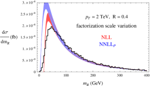
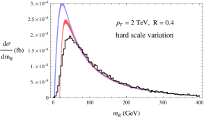
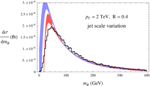
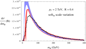
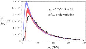
Figure 11: Scale uncertainties for $p_{T}=2$ TeV and $R=0.4$.

7 The Role of Non-Global Logarithms

As mentioned in Section 4, although we were able to refactorize the soft function into a soft-collinear part, whose natural scale is associated with the soft modes within the jet, the remainder soft function still depended on multiple scales $S_{r}=S_{r}(k_{\rm in},k_{\rm out},\mu)$. Thus we cannot guarantee that all large logarithms in the jet mass distribution are resummed. The residual dependence of the remainder soft function on two scales is the problem of non-global structure. In the absence of a complete understanding of non-global structure, and how the non-global logs (NGLs) might be resummed, we will content ourselves with an estimate of how non-global structure might affect the jet mass distribution. We start by drawing on the lessons learned when considering $e^{+}e^{-}\to$ dijets, where there have been several studies [19, 49, 57, 24, 25].

A two-loop calculation of the soft function for hemispherical jets was performed in [49, 57] and for cone or anti-$k_{T}$ jets, with an out-of-jet veto, in [25]. An intriguing observation from these studies is that in both examples, the NGLs arose from combinations of various logarithms of a single scale, coming from integrals in separate phase space regions. To give a specific example, in the calculation of the cumulative doubly differential dijet mass distribution for hemispherical jets, the details of which can be found in [49], it was shown that the leading non-global logarithm is of the form

$$-\frac{4\pi^{2}}{3}C_{F}C_{A}\ln^{2}\frac{E_{L}}{E_{R}}\;.$$ (51)

This is the coefficient of $\left(\frac{\alpha_{s}}{4\pi}\right)^{2}$ in the soft function, with $E_{L}$ and $E_{R}$ cumulant variables corresponding to integrals over $k_{L}={\bar{n}}\cdot P_{X_{L}}$ and $k_{R}=n\cdot P_{X_{R}}$, respectively, where $P_{X_{L}}$ and $P_{X_{R}}$ are the total momentum of the soft radiation propagating in the left or right hemispheres and $n=(1,\hat{n})$ denotes the thrust axis. This double logarithm came from the sum of three contributions from the two gluon real emission graphs off the two Wilson lines

$$\begin{tabular}[]{lcl}$\displaystyle-\frac{4\pi^{2}}{3}C_{F}C_{A}\ln^{2}\frac{E_{L}}{\mu}$&&{\rm both gluons in left hemisphere}\\[8.0pt] $\displaystyle-\frac{4\pi^{2}}{3}C_{F}C_{A}\ln^{2}\frac{E_{R}}{\mu}$&&{\rm both gluon in right hemisphere}\\[8.0pt] $\displaystyle+\frac{8\pi^{2}}{3}C_{F}C_{A}\ln\frac{E_{L}}{\mu}\ln\frac{E_{R}}{\mu}$&&{\rm one gluon in each hemisphere}\end{tabular}\;.$$

One therefore expects a similar sum of phase space regions to produce the leading non-global logarithm for the soft function we need in this paper.

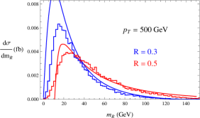
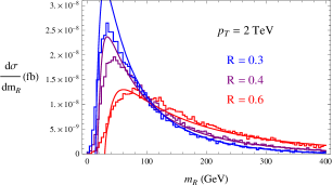
Figure 12: The resummed NLL jet mass distribution for different cone sizes for $p_{T}=500$ GeV and 2 TeV (curves) compared to pythia (histograms).

Now, we have already refactorized the soft function as

$$S(k_{\rm in},k_{\rm out},\mu)=\hat{S}(k_{\rm in},\mu)S_{r}(k_{\rm in},k_{\rm out},\mu)\;,$$ (52)

with the regional soft function $\hat{S}(k_{\rm in},\mu)$ defined to have all the radiation going into the jet. Thus we expect a double logarithm similar to the first term in Eq. (7) to contribute at two loops

$$\hat{S}(\kappa_{\rm in},\mu)=\cdots+\left(\frac{\alpha_{s}}{4\pi}\right)^{2}\Gamma^{\mathrm{NGL}}\ln^{2}\frac{\kappa_{\rm in}}{\mu}\;,$$ (53)

where $\Gamma^{\mathrm{NGL}}$ might be $-\frac{4\pi^{2}}{3}C_{F}C_{A}$, but is yet unknown. Since this term has $\mu$-dependence, it will contribute to the anomalous dimension of $\hat{S}$. Moreover, it will contribute a term with $\ln\mu$ in the anomalous dimension. This is unusual since, for a global observable, one normally expects that all of the $\ln\mu$ dependence in the anomalous dimension is proportional to $\gamma_{\rm cusp}$. We therefore expect similar non-cusp $\ln\mu$ dependence in the anomalous dimension of the regional soft function for the jet mass distribution as well.

With this educated guess, we expect that the two-loop regional soft function anomalous dimension for the annihilation channel has the form

$$\gamma_{\hat{S}}=\left(\frac{\alpha_{s}}{4\pi}\right)^{2}\left[\displaystyle\left(2C_{A}\Gamma_{1}+\Gamma^{\rm NGL}\right)\ln\left(\frac{1+\beta^{2}}{\beta}\frac{\kappa_{\rm in}}{\mu}\right)+C_{A}\gamma^{s}+\gamma^{\mathrm{NGL}}\right]$$ (54)

and similarly for the Compton channel, with $C_{F}\to C_{A}$ by Casimir scaling. Here, $\Gamma_{1}$ is the two-loop cusp anomalous dimension:

$$\Gamma_{1}=4\left(\frac{67}{9}-\frac{\pi^{2}}{3}\right)C_{A}-\frac{20}{9}n_{f}T_{F}\;,$$ (55)

and $\Gamma^{\mathrm{NGL}}$ and $\gamma^{\mathrm{NGL}}$ are unknown. By RG invariance, this implies that the anomalous dimension of the residual soft function must be

$$\gamma_{S_{r}}=\left(\frac{\alpha_{s}}{4\pi}\right)^{2}\left[\displaystyle-4C_{F}\Gamma_{1}\ln\left(\frac{1+\beta^{2}}{\beta}\frac{\kappa_{\rm out}}{\mu}\right)-\Gamma^{\rm NGL}\ln\left(\frac{1+\beta^{2}}{\beta}\frac{\kappa_{\rm in}}{\mu}\right)-2C_{F}\gamma^{s}-\gamma^{\mathrm{NGL}}\right]$$ (56)

where $\gamma_{s}$ is the two-loop direct-photon soft function anomalous dimension from[27]:

$$\gamma^{s}=\left(28\zeta_{3}-\frac{808}{27}+\frac{11\pi^{2}}{3}\right)C_{A}+\left(\frac{224}{27}-\frac{4\pi^{2}}{9}\right)n_{f}T_{F}\;.$$ (57)

The terms proportional to $\Gamma_{1}$ and $\gamma_{s}$ in Eq. (54) and Eq. (56), and also a known term proportional to the 3-loop cusp anomalous dimension, account for the global logarithms at NNLL. The $\Gamma^{\mathrm{NGL}}$ term parameterizing the unknown leading NGL. The $\gamma^{\mathrm{NGL}}$ anomalous dimension accounts for sub-leading NGLs, and the remaining non-global structure in the finite part of the two-loop soft function has effects which are formally N³LL.

Without performing a two-loop calculation, the expressions for $\Gamma^{\mathrm{NGL}}$ and $\gamma^{\mathrm{NGL}}$ are unknown. We estimate the effect of the missing terms by varying $\Gamma^{\mathrm{NGL}}$ between $\pm 100$, since $100\sim 4C_{F}\Gamma_{1}\sim\frac{8\pi^{2}}{3}C_{F}C_{A}$. The result of performing such a variation is shown in Figure 13. The band in this plot shows a reasonable expectation of the improvement one could expect if the leading non-global logarithm could be resummed. We see that the NGL only affects significantly the distribution in the peak region.

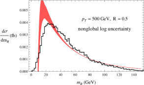
Figure 13: Estimation of the effect of leading non-global log resummation. Note that it affects significantly only the peak region of the distribution.

8 Conclusions

In this paper we have calculated the distribution of jet mass at a hadron collider, for events in which the jet recoils against a hard photon. Our calculation includes resummation at the next-to-leading logarithmic level (NLL) which involves both final state radiation of the jet and initial state radiation of the colliding partons. We also have included resummation of all the global logarithmic terms at next-to-next-to-leading logarithmic level producing a distribution we label NNLL_p (“p” for partial, since the non-global logarithmic terms have not been resummed). Our approach is based on expanding around the threshold limit, where the photon has very large momentum. By demanding the photon be hard, we force the hadronic final state to be that of a single jet for which a simple factorization formula exists. Our result is differential in the jet and photon rapidities and transverse momenta, although we assume the photon and jet have equal and opposite transverse momenta, which is true at leading power.

We have compared our theoretical calculation to the output from pythia, and find very good agreement. Although pythia is only formally accurate to the leading-logarithmic level, it has elements of subleading logarithms, and is expected to be in good agreement with collider data. Since we are able to include color coherence effects, from initial state radiation, as well as subleading logarithms, our calculation is more precise than pythia, as far as perturbative QCD is concerned. Since pythia also includes hadronization it is more likely to describe the data well for very small jet mass. It would be interesting to compare both directly to collider data from the LHC when it becomes available.

The two scales in our distribution, the photon $p_{T}$ and the jet mass $m_{R}$ lead to non-global logarithms. This is because in our approach there are two thresholds, $m_{R}\to 0$ and $m_{X}\to 0$, where $m_{X}$ is the mass of everything-but-the-photon. In particular, there are two soft scales, $k_{\rm in}$ associated with soft radiation in the jet, related to $m_{R}$, and $k_{\rm out}$ associated with radiation out of the jet, which can be related to $m_{X}^{2}-m_{R}^{2}$. Non-global logarithms of the ratio of these scales make resummation difficult beyond the NLL level. An alternative calculation would be to impose a jet veto at a scale similar to the soft scale. Then the non-global structure would reduce to a single number, which one might estimate or argue to be small. However, for an inclusive jet mass calculation, it seems impossible to avoid non-global structure and therefore resumming non-global logarithms is necessary for NNLL resummation.

Although we have not been able to resum the non-global logs in this paper, we found that if one ignores them completely, by choosing a single scale for the entire soft function, the distribution is completely wrong. This is because, using SCET alone, the two soft scales are not distinguished. Instead, we observe that contributions to the soft function coming from radiation going entirely into the jet can be consistently factorizes off. There are many ways to refactorize the soft function, and we make one particular choice, preserving the color structure associated with the hard directions. We give an operator definition to this regional soft function and calculate it at one loop. The regional soft function has a natural scale associated with soft/$n_{J}$-collinear modes. Allowing ourselves to pick two different soft scales, which we do numerically, gives a result which is in very good agreement with pythia, in the region that our calculation can be trusted.

There are many directions in which this work can be continued. It would be interesting to calculate the regional soft function at two loops, to see its non-global structure. One might hope that, since we expect an anomalous dimension for this soft function to have $\mu$ dependence related to the leading non-global logarithm, that with further insight non-global logarithms could be resummed. Then one could produce an NNLL calculation of jet mass. Other related applications would include a calculation of the jet mass in dijet events, for which there is already data [63] and the one-loop hard function and anomalous dimensions have already been prepared [64], or a calculation of jet mass in direct photon events including a jet veto. With a jet veto one can force single-jet kinematics well away from threshold and the size of the non-global structure can be controlled. However, the calculation would be significantly more complicated than what we have done here. In addition, it would be interesting to pursue the consideration of the jet mass distribution using different jet algorithms.

References

- [1] J. Butterworth, B. Cox, and J. R. Forshaw Phys.Rev. D65 (2002) 096014, [hep-ph/0201098].
- [2] J. M. Butterworth, A. R. Davison, M. Rubin, and G. P. Salam Phys.Rev.Lett. 100 (2008) 242001, [arXiv:0802.2470].
- [3] D. E. Kaplan, K. Rehermann, M. D. Schwartz, and B. Tweedie Phys.Rev.Lett. 101 (2008) 142001, [arXiv:0806.0848].
- [4] S. D. Ellis, C. K. Vermilion, and J. R. Walsh Phys.Rev. D81 (2010) 094023, [arXiv:0912.0033].
- [5] J. Thaler and L.-T. Wang JHEP 0807 (2008) 092, [arXiv:0806.0023].
- [6] D. Krohn, J. Thaler, and L.-T. Wang JHEP 1002 (2010) 084, [arXiv:0912.1342].
- [7] J. Gallicchio, J. Huth, M. Kagan, M. D. Schwartz, K. Black, et. al. JHEP 1104 (2011) 069, [arXiv:1010.3698].
- [8] J. Thaler and K. Van Tilburg JHEP 1103 (2011) 015, [arXiv:1011.2268].
- [9] J. Gallicchio and M. D. Schwartz Phys.Rev.Lett. 105 (2010) 022001, [arXiv:1001.5027].
- [10] Y. Cui, Z. Han, and M. D. Schwartz Phys.Rev. D83 (2011) 074023, [arXiv:1012.2077].
- [11] J. Gallicchio and M. D. Schwartz Phys.Rev.Lett. 107 (2011) 172001, [arXiv:1106.3076].
- [12] A. Altheimer, S. Arora, L. Asquith, G. Brooijmans, J. Butterworth, et. al. J.Phys.G G39 (2012) 063001, [arXiv:1201.0008].
- [13] S. D. Ellis, A. Hornig, T. S. Roy, D. Krohn, and M. D. Schwartz Phys.Rev.Lett. 108 (2012) 182003, [arXiv:1201.1914].
- [14] T. Becher and M. D. Schwartz JHEP 07 (2008) 034, [arXiv:0803.0342].
- [15] W. M.-Y. Cheung, M. Luke, and S. Zuberi Phys. Rev. D80 (2009) 114021, [arXiv:0910.2479].
- [16] S. D. Ellis, A. Hornig, C. Lee, C. K. Vermilion, and J. R. Walsh Phys. Lett. B689 (2010) 82–89, [arXiv:0912.0262].
- [17] T. T. Jouttenus Phys. Rev. D81 (2010) 094017, [arXiv:0912.5509].
- [18] S. D. Ellis, C. K. Vermilion, J. R. Walsh, A. Hornig, and C. Lee JHEP 11 (2010) 101, [arXiv:1001.0014].
- [19] A. Banfi, M. Dasgupta, K. Khelifa-Kerfa, and S. Marzani JHEP 08 (2010) 064, [arXiv:1004.3483].
- [20] Y.-T. Chien and M. D. Schwartz JHEP 08 (2010) 058, [arXiv:1005.1644].
- [21] R. Kelley, M. D. Schwartz, and H. X. Zhu arXiv:1102.0561.
- [22] T. T. Jouttenus, I. W. Stewart, F. J. Tackmann, and W. J. Waalewijn Phys.Rev. D83 (2011) 114030, [arXiv:1102.4344].
- [23] H.-n. Li, Z. Li, and C. P. Yuan Phys. Rev. Lett. 107 (2011) 152001, [arXiv:1107.4535].
- [24] K. Khelifa-Kerfa JHEP 1202 (2012) 072, [arXiv:1111.2016].
- [25] R. Kelley, M. D. Schwartz, R. M. Schabinger, and H. X. Zhu arXiv:1112.3343.
- [26] H.-n. Li, Z. Li, and C.-P. Yuan arXiv:1206.1344.
- [27] T. Becher and M. D. Schwartz JHEP 1002 (2010) 040, [arXiv:0911.0681]. 42 pages, 9 figures; v2: references added, minor changes; v3: typos; v4: typos, corrections in (16), (47), (72).
- [28] D. Appell, G. F. Sterman, and P. B. Mackenzie Nucl.Phys. B309 (1988) 259.
- [29] S. Catani, M. L. Mangano, and P. Nason JHEP 9807 (1998) 024, [hep-ph/9806484].
- [30] T. Becher, M. Neubert, and G. Xu JHEP 0807 (2008) 030, [arXiv:0710.0680].
- [31] T. Sjostrand, S. Mrenna, and P. Z. Skands JHEP 0605 (2006) 026, [hep-ph/0603175].
- [32] C. W. Bauer, S. Fleming, D. Pirjol, and I. W. Stewart Phys. Rev. D63 (2001) 114020, [hep-ph/0011336].
- [33] C. W. Bauer, D. Pirjol, and I. W. Stewart Phys. Rev. D65 (2002) 054022, [hep-ph/0109045].
- [34] L. G. Almeida, S. J. Lee, G. Perez, I. Sung, and J. Virzi Phys.Rev. D79 (2009) 074012, [arXiv:0810.0934].
- [35] Report 2011 (2011).
- [36] M. Dasgupta and G. P. Salam Phys. Lett. B512 (2001) 323–330, [hep-ph/0104277].
- [37] M. Dasgupta and G. P. Salam JHEP 03 (2002) 017, [hep-ph/0203009].
- [38] A. Banfi, G. Marchesini, and G. Smye JHEP 08 (2002) 006, [hep-ph/0206076].
- [39] R. B. Appleby and M. H. Seymour JHEP 12 (2002) 063, [hep-ph/0211426].
- [40] T. Becher, C. Lorentzen, and M. D. Schwartz Phys.Rev.Lett. 108 (2012) 012001, [arXiv:1106.4310].
- [41] T. Becher, C. Lorentzen, and M. D. Schwartz arXiv:1206.6115.
- [42] T. Sjostrand, S. Mrenna, and P. Z. Skands Comput.Phys.Commun. 178 (2008) 852–867, [arXiv:0710.3820].
- [43] A. Banfi and M. Dasgupta Phys. Lett. B628 (2005) 49–56, [hep-ph/0508159].
- [44] Y. Delenda, R. Appleby, M. Dasgupta, and A. Banfi JHEP 0612 (2006) 044, [hep-ph/0610242].
- [45] R. Kelley, J. R. Walsh, and S. Zuberi arXiv:1202.2361.
- [46] R. Kelley, J. R. Walsh, and S. Zuberi arXiv:1203.2923.
- [47] C. W. Bauer, S. Fleming, and M. E. Luke Phys.Rev. D63 (2000) 014006, [hep-ph/0005275].
- [48] C. W. Bauer and I. W. Stewart Phys.Lett. B516 (2001) 134–142, [hep-ph/0107001].
- [49] R. Kelley, M. D. Schwartz, R. M. Schabinger, and H. X. Zhu Phys. Rev. D84 (2011) 045022, [arXiv:1105.3676].
- [50] N. Kidonakis, G. Oderda, and G. F. Sterman Nucl.Phys. B531 (1998) 365–402, [hep-ph/9803241].
- [51] C. F. Berger, T. Kucs, and G. F. Sterman Phys.Rev. D68 (2003) 014012, [hep-ph/0303051].
- [52] G. F. Sterman hep-ph/9606312.
- [53] J. C. Collins, D. E. Soper, and G. F. Sterman Adv.Ser.Direct.High Energy Phys. 5 (1988) 1–91, [hep-ph/0409313].
- [54] N. Kidonakis, G. Oderda, and G. F. Sterman Nucl.Phys. B525 (1998) 299–332, [hep-ph/9801268].
- [55] N. Kidonakis and G. F. Sterman Nucl.Phys. B505 (1997) 321–348, [hep-ph/9705234].
- [56] M. D. Schwartz Phys. Rev. D77 (2008) 014026, [arXiv:0709.2709].
- [57] A. Hornig, C. Lee, I. W. Stewart, J. R. Walsh, and S. Zuberi JHEP 08 (2011) 054, [arXiv:1105.4628].
- [58] M. Dasgupta, K. Khelifa-Kerfa, S. Marzani, and M. Spannowsky arXiv:1207.1640.
- [59] A. V. Manohar and I. W. Stewart Phys.Rev. D76 (2007) 074002, [hep-ph/0605001].
- [60] S. Catani and M. H. Seymour Phys. Lett. B378 (1996) 287–301, [hep-ph/9602277].
- [61] A. Martin, W. Stirling, R. Thorne, and G. Watt Eur.Phys.J. C63 (2009) 189–285, [arXiv:0901.0002].
- [62] J. M. Campbell and R. Ellis Nucl.Phys.Proc.Suppl. 205-206 (2010) 10–15, [arXiv:1007.3492].
- [63] Tech. Rep. ATLAS-CONF-2011-073, CERN, Geneva, May, 2011.
- [64] R. Kelley and M. D. Schwartz Phys.Rev. D83 (2011) 045022, [arXiv:1008.2759].