Vortex-density fluctuations, energy spectra and vortical regions in superfluid turbulence

Abstract

Measurements of the energy spectrum and of the vortex-density fluctuation spectrum in superfluid turbulence seem to contradict each other. Using a numerical model, we show that at each instance of time the total vortex line density can be decomposed into two parts: one formed by metastable bundles of coherent vortices, and one in which the vortices are randomly oriented. We show that the former is responsible for the observed Kolmogorov energy spectrum, and the latter for the spectrum of the vortex line density fluctuations.

Below a critical temperature, liquid helium becomes a two-fluid system in which an inviscid superfluid component coexists with a viscous normal fluid component. The flow of the superfluid is irrotational: superfluid vorticity is confined to vortex lines of atomic thickness around which the circulation takes a fixed value $\kappa$ (the quantum of circulation). Superfluid turbulence Vinen-Niemela ; Skrbek-Sreeni is easily created by stirring either helium isotope (⁴He or ³He-B), and consists of a tangle of reconnecting vortex filaments which interact with each other and with the viscous normal fluid (which may be laminar or turbulent). The most important observable quantity is the vortex line density $L$ (vortex length per unit volume), from which one infers the average distance between vortex lines, $\ell\approx L^{-1/2}$. Our interest is in the properties of superfluid turbulence and their similarities with ordinary turbulence.

Experiments Maurer ; Salort have revealed that, if the superfluid turbulence is driven by grids or propellers, the distribution of the turbulent kinetic energy over length scales larger than $\ell$ obeys the celebrated $k^{-5/3}$ Kolmogorov scaling observed in ordinary (classical) turbulence. Here $k$ is the magnitude of the three-dimensional wavenumber (wavenumber and frequency are related by $k=f/{\bar{v}}$, where ${\bar{v}}$ is the mean flow). Numerical calculations performed using either the vortex filament model Araki ; Baggaley-fluctuations or the Gross-Pitaevskii equation Nore ; Kobayashi confirm the Kolmogorov scaling. It is thought that the effect arises from the partial polarization of the vortex lines Vinen-Niemela ; Skrbek-Sreeni ; Lvov , but such effect has never been clearly identified. Another important experimental observation is that in both ⁴He Roche2007 and ³He-B Bradley2008 , the frequency spectrum of the fluctuations of $L$ has a decreasing $f^{-5/3}$ scaling typical of passive objects Roche-Barenghi ; Baggaley-fluctuations advected by a turbulent flow. This latter result seems to contradict the interpretation of $L$ as a measure of superfluid vorticity, $\omega=\kappa L$ which is usually made in the literature Stalp1999 ; Golov2008 ; Skrbek2010 ; Bradley2008 ; Vinen-Niemela ; Skrbek-Sreeni .

In fact, from dimensional analysis, the vorticity spectrum corresponding to the Kolmogorov law should increase with $f$ (as $f^{1/3}$), not decrease. Since the vortex line density is a positive quantity, a better analogy is to the enstrophy spectrum: however in classical turbulence this spectrum is essentially flat Ishihara ; Zhou , in disagreement with the helium experiments Roche2007 ; Bradley2008 .

The aim of this letter is to reconcile these two sets of observations (each separately backed by numerical simulations). We shall show that, at any instant, the vortex tangle can be decomposed into two parts: vortex lines which are locally polarised in the same direction, forming metastable coherent bundles, and vortex lines which are randomly oriented in space. The former is responsible for the Kolmogorov energy spectrum, and the latter for frequency spectrum of the vortex line density.

Following Schwarz Schwarz , we model vortex filaments as space curves ${\bf{s}}(\xi,t)$ which move according to

$$\frac{d{\bf s}}{dt}={\bf{v}}_{s}+\alpha{\bf{s}}^{\prime}\times({\bf{v}}_{n}-{\bf{v}}_{s})-\alpha^{\prime}{\bf{s}}^{\prime}\times\left({\bf{s}}^{\prime}\times\left({\bf{v}}_{n}-{\bf{v}}_{s}\right)\right),$$ (1)

where $t$ is time, $\alpha$ and $\alpha^{\prime}$ are known temperature dependent friction coefficients Donnelly-Barenghi , ${\bf{s}}^{\prime}=d{\bf{s}}/d\xi$ is the unit tangent vector at the point ${\bf{s}}$, $\xi$ is arc length, and ${\bf{v}}_{n}$ is the normal fluid velocity at the point $\bf s$. We set the temperature to $T=1.9~{}\rm K$, typical of many finite temperature studies (corresponding to $\alpha=0.206$ and $\alpha^{\prime}=0.0083$). The self-induced velocity of the vortex line at the point ${\bf{s}}$ is given by the Biot-Savart law Saffman

$${\bf{v}}_{s}({\bf{s}},\,t)=-\frac{\kappa}{4\pi}\oint_{\cal L}\frac{({\bf{s}}-{\bf{r}})}{|{\bf{s}}-{\bf{r}}|^{3}}\times{\bf d}{\bf{r}},$$ (2)

where $\kappa=9.97\times 10^{-4}~{}\rm cm^{2}/s$ (in ⁴He) and the line integral extends over the entire vortex configuration ${\cal L}$. The calculation is performed in a periodic cube of size $D=0.1~{}\rm cm$. The numerical techniques to discretize the vortex lines into a number of points ${\bf{s}}_{j}$ ($j=1,\cdots N$) held at minimum separation $\Delta\xi/2$, compute the time evolution, de-singularize the Biot-Savart integrals, evaluate ${\bf{v}}_{s}$ using a tree-method (with critical opening angle $0.4$), and algorithmically perform vortex reconnections when vortex lines come sufficiently close to each other, are all described in our previous papers Baggaley-fluctuations ; Baggaley-reconnections . Here we take $\Delta\xi=2\times 10^{-3}~{}$cm and a timestep of $5\times 10^{-5}~{}$s. The number of discretization points varies with time; in the statistically steady state we focus on, $N\approx 4000$.

The turbulent normal fluid is modelled by the following synthetic turbulent flow Osborne :

$${\bf{v}}_{n}({\bf{s}},\,t)=\sum_{m=1}^{M}({\bf A}_{m}\times{\bf{k}}_{m}\cos{\phi_{m}}+{\bf B}_{m}\times{\bf{k}}_{m}\sin{\phi_{m}}),$$ (3)

where $\phi_{m}={\bf{k}}_{m}\cdot{\bf{s}}+f_{m}t$, ${\bf{k}}_{m}$ and $f_{m}=\sqrt{k^{3}_{m}E(k_{m})}$ are wave vectors and angular frequencies. This flow is solenoidal and time-dependent; with a suitable random choice of ${\bf A}_{m}$, ${\bf B}_{m}$ and ${\bf{k}}_{m}$ (adapted to the periodic box). The normal fluid’s energy spectrum has Kolmogorov form $E(k_{m})\sim k_{m}^{-5/3}$ in the range from $k_{1}$ (corresponding to the integral scale) to $k_{M}$ (corresponding to the dissipation scale). This synthetic model of turbulence compares very well with Lagrangian statistics obtained in direct numerical simulations of the Navier-Stokes equations and experiments. Here we take $M=188$, $k_{1}=0.1~{}\rm cm$ and $k_{M}=1.8\times 10^{-3}~{}\rm cm$, which corresponds to the Reynolds number $\mbox{\rm Re}_{n}=(k_{1}/k_{M})^{4/3}\approx 200$. For computational simplicity our model ignores any back-reaction of the vortex lines onto the normal fluid.

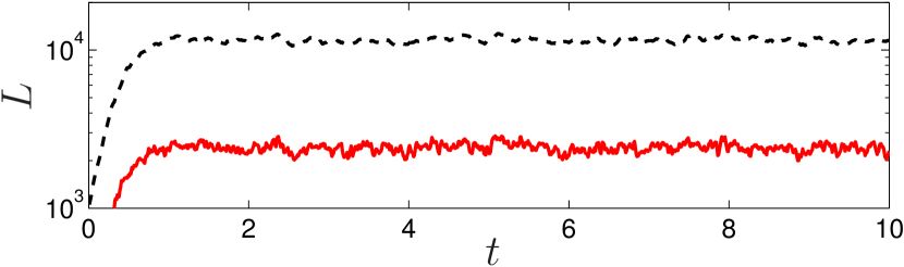
Figure 1: (Color online) The time evolution of the total vortex line density (black dashed line) $L$ ($\rm cm^{-2}$) and the polarised component $L_{\parallel}$ ($\rm cm^{-2}$) (solid red line).

We integrate the vortex lines in time according to Eq. (1), for a period of $10~{}\rm s$ (approximately 25 large eddy turnover times of the normal fluid). We find that, after an initial transient, the vortex line density saturates to a statistically steady state, as shown in Fig. 1, independently of the initial condition (various vortex loop configurations were tried).

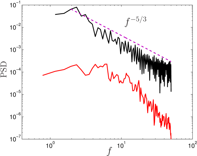
Figure 2: (Color online). Power spectral density, PSD, (arbitrary units) of fluctuations of the total vortex line density $L$ (black upper solid line) and of the polarised vortex line density $L_{\parallel}$ (red lower solid line) vs frequency $f$ ($\rm s^{-1}$). The dashed (magenta) line shows the $f^{-5/3}$ scaling.

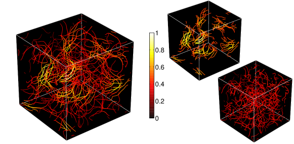
Figure 3: (Color online) Left: Snapshot of the vortex tangle at $t=7\,$s. Vortex lines are locally coloured according to the local magnitude of the smoothed vorticity field $\omega$. Right: The same snapshot but split into the locally polarized (top, ${\omega}({\bf{s}}_{i})>1.4\omega_{\rm rms}$) and random components (bottom, ${\omega}({\bf{s}}_{i})<1.4\omega_{\rm rms}$) respectively. The color scale is normalised by the maximum value $\omega_{\rm max}=38.4\,$s^-1; $\omega_{\rm rms}=15.7\,$s^-1

.

We analyse the properties of the superfluid turbulence in the statistically steady state ($t\gtrsim 1.2\,$s). Firstly, we compute the frequency spectrum of the fluctuations of the vortex line density about its average value $<L>=1.15\times 10^{4}~{}\rm cm^{-2}$. Fig. 2 shows that the spectrum scales as $f^{-5/3}$ for large $f$, as observed in experiments Roche2007 ; Bradley2008 and numerical simulations Baggaley-fluctuations . Secondly, we compute the superfluid energy spectrum $E(k)$, defined by

$$\frac{1}{|V|}\int_{V}\frac{1}{2}|{\bf v}_{s}|^{2}d{\bf x}=\int E(k)dk,$$ (4)

where $V=D^{3}$ is volume. The top curve (labelled a) of Fig. 4 shows that the energy spectrum (computed on a $256^{3}$ Cartesian mesh) is consistent with the cascading classical Kolmogorov scaling $E(k)\sim k^{-5/3}$ in the range $k_{D}=2\pi/D<k<k_{\ell}=2\pi/{\ell}$, in agreement with experiments Maurer ; Salort and numerical simulations Araki ; Baggaley-fluctuations ; Nore ; Kobayashi ; at larger wavenumbers $k>k_{\ell}$ the spectrum exhibits the non-cascading scaling of individual vortex lines. We conclude that the numerical model reproduces the two major spectral features (the energy spectrum and the vortex density fluctuations spectrum) observed in superfluid turbulence.

To solve the puzzle described in the introduction, we examine the homogeneity of the turbulence. A simple three-dimensional plot of the vortex lines may give the wrong impression that the vortex tangle is spatially uniform: the orientation of the lines is not apparent and some lines partially hide each other. A more careful analysis is required. We define a smoothed vorticity field $\omega$ at the discretization points ${\bf{s}}_{j}$ using a kernel with finite support, the $M_{4}$ kernel Monaghan-Review (effectively a cubic spline):

$${\mbox{\boldmath$\omega$}}({\bf{s}}_{i})=\kappa\sum_{j=1}^{N}{\bf{s}}^{\prime}_{j}W(r_{ij},h)\Delta\xi_{j},$$ (5)

where $r_{ij}=|{\bf{s}}_{i}-{\bf{s}}_{j}|$, $\Delta\xi_{j}=|{\bf{s}}_{j+1}-{\bf{s}}_{j}|$, $W(r,h)=g(r/h)/(\pi h^{3}),$ $h$ is a characteristic length scale, and

$$g(q)=\begin{cases}1-\frac{3}{2}q^{2}+\frac{3}{4}q^{3},&0\leq q<1;\\ \frac{1}{4}\left(2-q\right)^{3},&1\leq q<2;\\ 0,&q\geq 2.\end{cases}$$ (6)

This approach is commonly employed in the smoothed particle hydrodynamics (SPH) literature Monaghan-Review , as we only need to take the contribution of discretization points within a radius of $2h$ from each point ${\bf{s}}_{i}$. We tested this smoothing algorithm against a Gaussian kernel $g(q)=e^{-q^{2}}$ Baggaley-structures and found comparable results for single snapshots of the vortex tangle. The advantage of the new algorithm is that $\omega$ is computed only at the discretization points, so it can be evaluated during the time evolution.

Setting $h=\ell$, the smoothed vorticity field $\omega$ allows us to identify the presence of any coherent vortex structures. From the vorticity values ${\mbox{\boldmath$\omega$}}_{j}$ at each discretization point ${\bf{s}}_{j}$ we compute the rms vorticity $\omega_{\rm rms}=\sqrt{\frac{1}{N}\sum_{i=1}^{N}|{{\mbox{\boldmath$\omega$}}}({\bf{s}}_{i})|^{2}}.$ and, following Ref. Roche-Barenghi , we decompose the vortex lines into locally ‘polarised’ and ‘unpolarised‘ fields, $L_{\parallel}$ and $L_{\times}$ respectively. The polarised vortex line density $L_{\parallel}$ consists of the discretization points ${\bf{s}}_{j}$ associated to intense metastable vortical regions where the magnitude of the smoothed vorticity exceeds the rms vorticity by a threshold value, $\omega({\bf{s}}_{i})>1.4\omega_{\rm rms}$ (we shall discuss this threshold shortly). The remaining discretization points form the ‘unpolarised’ field $L_{\times}$. As with the total vortex line density, we find that $L_{\parallel}$ rapidly saturates to a statistically steady state, see Fig. 1.

A snapshot of the vortex tangle in which the vortex lines are coloured according to the local value of the smoothed vorticity is shown in Fig. 3 (left); vortex bundles are clearly visible. The right-hand side of Fig. 3 shows respectively the polarised (top, $\omega({\bf{s}}_{j})>1.4\omega_{\rm rms}$) and unpolarised vortex lines (bottom, $\omega({\bf{s}}_{j})<1.4\omega_{\rm rms}$): the former consists of bundles and contributes to $L_{\parallel}$, the latter is spatially random and contributes to $L_{\times}$.

We find that the polarised and unpolarised vortex lines have different properties. The frequency spectrum of the fluctuations of $L_{\times}$ scales as $f^{-5/3}$, as for the total line density $L$ (top black curve of Fig. 2), whereas the spectrum of the fluctuations of $L_{\parallel}$ slowly increases at low frequency and drops rapidly at high frequency (bottom red curve of Fig. 2). Changing the threshold value within the range 1.4 to 2.2$\omega_{\rm rms}$ does not change this distinction. The flattening and the slow increase with $f$ of the spectrum of the fluctuations of the polarised vortex lines are consistent with observations in ordinary turbulence Ishihara ; Zhou .

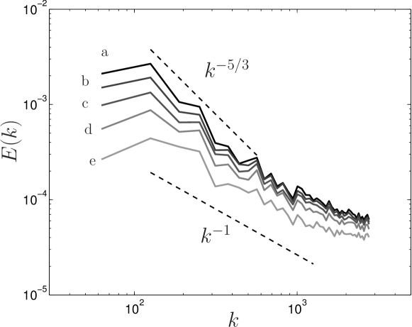
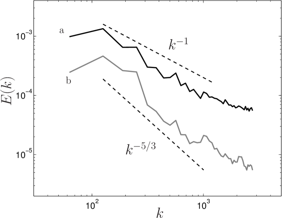
Figure 4: Energy spectra $E(k)$ (arbitrary units) vs wavenumber $k$ ($\rm cm^{-1}$) corresponding to Fig. 3. Top: The upper solid line (a) is the energy spectrum corresponds to the flow induced by all vortex lines. Lower curves correspond to the flow induced by vortices with smoothed vorticity below the following thresholds: (b) $\omega<1.7\omega_{rms}$, (c) $1.4\omega_{rms}$, (d) $1.2\omega_{rms}$, and (e) $\omega_{rms}$. Bottom: Energy spectra corresponding to vortex lines with smoothed vorticity respectively below (a) and above (b) the threshold $1.4\omega_{rms}$. The dashed lines display the $k^{-1}$ and the $k^{-5/3}$ scalings.

We now turn our attention to the role of the polarised lines on the energy spectrum. We have seen that the top curve (labelled a) of the top panel of Fig. 4 displays, in the range $k_{D}<k<k_{\ell}$, the Kolmogorov energy spectrum corresponding to all vortex lines. The curves labelled b, c, d, and e show energy spectra arising only from discretization points ${{\bf{s}}_{j}}$ such that $\omega$ is below a given (decreasing) rms threshold. It is clear that, as we remove the contribution of the high-intensity bundles, the energy spectrum $E(k)$ in the range $k_{D}<k<k_{\ell}$ becomes shallower, and changes from a $k^{-5/3}$ scaling to a $k^{-1}$ scaling. The bottom panel of Fig. 4 compares the energy spectrum arising from the isotropic vorticity $L_{\times}$ (top curve, labelled a) and that arising from the polarised vorticity $L_{\parallel}$ (bottom curve, labelled b). It is apparent that the vortex bundles correspond to the classical $k^{-5/3}$ Kolmogorov scaling, and that the random vorticity corresponds to the $k^{-1}$ spectrum.

The decomposition of $L$ into $L_{\parallel}$ and $L_{\times}$ is robust and holds during the time evolution, thus vindicating Roche and Barenghi Roche-Barenghi who suggested it when discussing an experiment Roche2007 . Unlike that experiment, in our calculation the random vortex lines contain most of the energy. A possible explanation of this difference is that our model of turbulent normal fluid does not contain strong vortical structures, unlike real turbulence or DNS, thus our polarised bundles are an underestimate of reality (the presence of vortical structures in the normal fluid would certainly induce stronger vortex bundles in the superfluid, as shown in numerical simulations Koplik-Morris , hence increase the energy contained in $L_{\parallel}$). It is also interesting to remark that the the smoothed vorticity $\omega$ can be related to the coarse-grained vorticity of the HVBK equations HVBK , and that the decomposition of $L$ into $L_{\parallel}$ and $L_{\times}$, has an analogy to that of Farge et al. Farge for classical turbulence.

In summary, we have shown compelling evidence that, at any instant, the turbulent vortex tangle can be decomposed into a polarised and a random component. The polarised component, associated to $L_{\parallel}$, consists of metastable coherent vortex bundles, shown in the top right panel of Fig. 3, and is responsible for the observed Kolmogorov $k^{-5/3}$ energy spectrum. The random component, shown in the bottom right panel of Fig. 3, is responsible for the observed $f^{-5/3}$ frequency spectrum of the fluctuations of the vortex length. The result confirms that the Kolmogorov spectrum arises from partial polarization of the vortex lines, and solves an apparent puzzle between experiments. It also points to direction of further work: determining the degree of polarization as a function of temperature and normal fluid’s Reynolds number (in Fig. 1 it is about 20 percent with the parameters used), and developing a two-scale approach to superfluid hydrodynamics such as Lipniacki’s Lipniacki to account for such polarization.

This work was supported by the Leverhulme Trust, grant numbers F/00 125/AH and F/00 125/AD, and the ANR program STATOCEAN (ANR-09-SYSC-014). AWB acknowledges helpful discussions with Paul Clark.

References

- (1) W.F. Vinen, and J.J. Niemela, J. Low Temp. Phys.128, 167 (2002).
- (2) L. Skrbek and K. R. Sreenivasan, Physics of Fluids 24, 011301 (2012).
- (3) J. Maurer and P. Tabeling, Europhys. Lett. 43, 29 (1998).
- (4) J. Salort et al., Phys. of Fluids 22, 125102 (2010).
- (5) T. Araki, M. Tsubota, and S.K. Nemirovskii, Phys. Rev. Lett. 89, 14, (2002).
- (6) A.W. Baggaley and C.F. Barenghi, Phys. Rev. B 84, 020504 (2011).
- (7) C. Nore, M. Abid, and M.-E. Brachet, Phys. Rev. Lett. 78, 3896 (1997).
- (8) M. Kobayashi, and M. Tsubota, Phys. Rev. Lett. 94, 065302 (2005).
- (9) V.S. L’vov, S.V. Nazarenko, and O. Rudenko, Phys. Rev. B 76, 024520 (2007).
- (10) P.-E. Roche, P. Diribarne, T. Didelot, O. Français, L. Rousseau, and H. Willaime, Europhys. Lett. 77 66002 (2007).
- (11) D.I. Bradley, S.N. Fisher, A.M. Gunault, R.P. Haley, S. O’Sullivan, G.R. Pickett, and V. Tsepelin, Phys. Rev. Lett. 101, 065302 (2008).
- (12) P.-E. Roche and C.F. Barenghi, Europhys. Lett. 81, 36002 (2008).
- (13) S.R. Stalp, L. Skrbek, and R.J. Donnelly, Phys. Rev. Lett. 82, 4831 (1999).
- (14) P.M. Walmsley and A.I. Golov, Phys. Rev. Lett. 100, 245301 (2008).
- (15) L. Skrbek, J. Low Temp. Phys. 161, 555 (2010).
- (16) T. Ishihara, Y. Kaneda, M. Yokokawa, K. Itakura, and A. Uno, J. Phys. Soc. Jpn 72 983 (2003).
- (17) T. Zhou, R.A. Antonia, and L.P. Chua, J. of Turbulence 6, 28 (2005).
- (18) K.W. Schwarz, Phys. Rev. B 38, 2398 (1988).
- (19) R.J. Donnelly and C.F. Barenghi, J. Phys. Chem. Ref. Data 27, 1217, (1998).
- (20) P.G. Saffman, Vortex Dynamics (Cambridge University Press, Cambridge, England, 1992).
- (21) A.W. Baggaley, J. Low Temp. Physics 168, 18, (2012).
- (22) D.R. Osborne, J.C. Vassilicos, K. Sung, and J.D. Haigh, Phys. Rev. E 74, 036309, (2006).
- (23) J.J. Monaghan, Annu. Rev. Astron. Astr. 30, 543, (1992).
- (24) A.W. Baggaley, C.F. Barenghi, A. Shukurov, and Y.A. Sergeev, Europhys. Lett. 98, 26002, (2012).
- (25) K. Morris, J. Koplik, and D. Rouson, Phys. Rev. Lett. 101, 015301 (2008).
- (26) H.E. Hall and W.F. Vinen, Proc. Roy. Soc. London, Ser. A 238, 215 (1954); I.I. Bekharavich and I.M. Khalatnikov, Zh. Eksp. Teor. Fiz. 40, 920 (1961) [Sov. Phys. JETP 13, 643 (1961)]; R.N. Hills and P.H. Roberts, Arch. Rat. Mech. Anal. 66, 43 (1977).
- (27) M. Farge, K. Schneider, G. Pellegrino, A.A. Wray and R.S. Rogallo, Phys. of Fluids 15, 2886, (2003).
- (28) T. Lipniacki, Europ. J. Mechanics B/Fluids, 25, 435 (2006).