Pion-nucleon elastic scattering amplitude within covariant baryon chiral perturbation theory up to $O(p^{4})$ level

Abstract

The $O(p^{4})$ calculation on pion-nucleon elastic scattering amplitude in EOMS scheme within covariant baryon chiral perturbation theory is reviewed. Numerical fits to partial wave amplitudes up to $\sqrt{s}=1.13$GeV and $1.20$GeV are performed and the results are compared with previous studies.

1 Introduction

Many efforts have been made in studying $\pi$-$N$ scatterings at low energies. However, unlike the successfulness of chiral perturbation theory in pure mesonic sector, a chiral expansion in $\pi$-$N$ scattering amplitude suffers from the power counting breaking (PCB) problem in the traditional subtraction $\overline{MS}-1$ scheme. [1] Many proposals have been made to treat this problem, e.g., heavy baryon chiral perturbation theory [2], infrared regularization scheme [3], extended on mass shell (EOMS) scheme [4], etc.. The EOMS scheme provides a good solution to the PCB problem, e.g., see [5], in the sense that it faithfully respects the analytic structure of the original amplitudes and being scale independent.

In this talk we will present our work on the $O(p^{3})$ and $O(p^{4})$ calculation on $\pi$-$N$ scattering amplitude in EOMS scheme and will compare it with previous results in the literature.

2 NNLO and NNNLO calculations

Table 1: Fitting results at ${\cal O}(p^{3})$ and ${\cal O}(p^{4})$. Given for comparison are results from [7, 9]. The $c_{i}$, $d_{j}$ and $e_{k}$ have, respectively, units of $\rm{GeV}^{-1}$, $\rm{GeV}^{-2}$ and $\rm{GeV}^{-3}$. In ${\cal O}(p^{4})$ fits, the fitted $c_{i}$ here should be understood as $\hat{c_{i}}$: $\hat{c_{1}}=c_{1}-2M^{2}\left(e_{22}-4e_{38}\right)$, $\hat{c_{2}}=c_{2}+8M^{2}\left(e_{20}+e_{35}\right)$, $\hat{c_{3}}=c_{3}+4M^{2}\left(2e_{19}-e_{22}-e_{36}\right)$, $\hat{c_{4}}=c_{4}+4M^{2}\left(2e_{21}-e_{37}\right)$.

LEC	Fit I-${\cal O}(p^{3})$	Ref. [7]-${\cal O}(p^{3})$	Fit II-${\cal O}(p^{3})$	Ref. [9]-${\cal O}(p^{3})$	Fit I-${\cal O}(p^{4})$	Fit II-${\cal O}(p^{4})$
$c_{1}$	$-1.39\pm 0.06$	$-1.50\pm 0.06$	$-0.81\pm 0.03$	$-1.00\pm 0.04$	$-1.09\pm 0.06$	$-0.98\pm 0.03$
$c_{2}$	$4.00\pm 0.09$	$3.74\pm 0.09$	$1.46\pm 0.09$	$1.01\pm 0.04$	$2.79\pm 0.10$	$1.41\pm 0.04$
$c_{3}$	$-6.59\pm 0.08$	$-6.63\pm 0.08$	$-3.09\pm 0.12$	$-3.04\pm 0.02$	$-5.32\pm 0.14$	$-3.76\pm 0.04$
$c_{4}$	$3.91\pm 0.04$	$3.68\pm 0.05$	$2.35\pm 0.06$	$2.02\pm 0.01$	$2.38\pm 0.19$	$1.16\pm 0.03$
$d_{1}+d_{2}$	$4.32\pm 0.53$	$3.67\pm 0.54$	$0.78\pm 0.09$		$6.21\pm 0.12$	$2.14\pm 0.04$
$d_{3}$	$-3.00\pm 0.50$	$-2.63\pm 0.51$	$-0.46\pm 0.05$		$-6.86\pm 0.16$	$-3.88\pm 0.05$
$d_{5}$	$-0.56\pm 0.13$	$-0.07\pm 0.13$	$-0.16\pm 0.04$		$0.54\pm 0.11$	$1.17\pm 0.04$
$d_{14}-d_{15}$	$-7.05\pm 1.05$	$-6.80\pm 1.07$	$-0.89\pm 0.15$		$-11.90\pm 0.24$	$-3.96\pm 0.08$
$d_{18}$	$-0.74\pm 1.41$	$-0.50\pm 1.43$	$-0.92\pm 0.25$		$-0.74$(input)	$-0.74$(input)
$e_{14}$	-	-	-	-	$3.68\pm 0.36$	$2.62\pm 0.09$
$e_{15}$	-	-	-	-	$-14.67\pm 0.55$	$-5.15\pm 0.13$
$e_{16}$	-	-	-	-	$7.15\pm 0.35$	$1.55\pm 0.07$
$e_{17}$	-	-	-	-	$0.57\pm 1.34$	$13.57\pm 0.15$
$e_{18}$	-	-	-	-	$3.64\pm 1.18$	$-9.05\pm 0.12$
$h_{A}$	-	-	$2.82\pm 0.04$	$2.87\pm 0.04$	-	$2.82$(input)
$\chi^{2}_{d.o.f}$	0.18	$0.22$	0.35	0.23	0.04	0.21

We start from the following effective lagrangian at $O(p^{3})$ level (extendable to $O(p^{4})$ [6]):

$${\cal L}_{eff} = \bar{N}\left\{i\,\not{D}-m+\frac{g_{A}}{2}\,\not{u}\gamma_{5}+c_{i}\,{\cal O}^{(2)}_{i}+d_{j}\,{\cal O}^{(3)}_{j}\right\}N+$$

$$\frac{f_{\pi}^{2}}{4}\langle u^{\mu}u_{\mu}+\chi_{+}\rangle+\frac{\ell_{4}}{8}\langle u^{\mu}u_{\mu}\rangle\langle\chi_{+}\rangle+\frac{\ell_{3}+\ell_{4}}{16}\langle\chi_{+}\rangle^{2}\ ,$$

where ${\cal O}^{(2)}$ and ${\cal O}^{(3)}$ are relevant operators of $O(p^{2})$ and $O(p^{3})$ respectively, $i\in(1,2,3,4)$ and $j\in(1,2,3,5,14,15,16,18)$ [6].

Decomposition of $\pi$-$N$ amplitude is standard,

$$T_{\pi N}^{a^{\prime}a} = \delta_{a^{\prime}a}T^{+}+\frac{1}{2}[\tau_{a^{\prime}},\tau_{a}]T^{-},$$

$$T^{\pm} = \bar{u}(p^{\prime},s^{\prime})\left[D^{\pm}+{i\over 2m_{N}}\sigma^{\mu\nu}q_{\mu}^{\prime}q_{\nu}B^{\pm}\right]u(p,s)\ .$$ (1)

To carry out the calculation in EOMS scheme one firstly perform $\overline{MS}-1$ substraction to remove ultraviolet divergencies, then additional substraction (A.S.) to absorb PCB terms. Taking the nucleon mass renormalization for example, one has,

$$m_{N} = m-4c_{1}M^{2}-\frac{3mg^{2}}{2f^{2}}\left[\Delta_{N}-M^{2}I(m^{2})\right]$$ (2)

$$= \mathring{m}-4c_{1}^{r}M^{2}+\frac{3mM^{2}g^{2}}{2f^{2}}\bar{I}(m^{2})\qquad\qquad\quad(\rm{\overline{{MS}}-1})$$

$$= \mathring{m}-4\tilde{c_{1}}M^{2}+\frac{3mM^{2}g^{2}}{2f^{2}}\overline{I}(m^{2})-{\frac{3mM^{2}g^{2}}{32\pi^{2}f^{2}}}\,(\rm{A.S.}),$$

where $\mathring{m}$ is the nucleon mass in chiral limit. The last term on the $r.h.s.$ of the third equality is opposite to the PCB term which is absorbed by redefining $c_{1}^{r}$ as: $\tilde{c_{1}}=c_{1}^{r}-\frac{3g^{2}m}{128f^{2}\pi^{2}}$. Definitions of all functions appeared here follow from A.

Another example is the calculation of the axial-vector coupling $g_{A}$:

$$g_{A} = g+4d_{16}M^{2}-\frac{g^{3}m^{2}}{32f^{2}\pi^{2}}+\frac{g(4-g^{2})}{2f^{2}}\Delta_{N}-\frac{g(2+g^{2})}{2f^{2}}\Delta_{\pi}$$ (3)

$$+ \frac{g^{3}(2m^{2}+M^{2})}{4f^{2}}J_{N}(0)-\frac{g(8-g^{2})M^{2}}{4f^{2}}I(m^{2})-\frac{g^{2}M^{4}}{4f^{2}}I_{A}(0)$$

$$+ \frac{3g^{3}m^{2}M^{2}}{f^{2}}\frac{\partial I(s)}{\partial s}I(s)\bigg{|}_{\not{p}=m_{N}}$$

$$= \mathring{g}_{A}+4d_{16}M^{2}-\frac{g(2+g^{2})}{2f^{2}}\Delta_{\pi}+\frac{3g^{3}m^{2}M^{2}}{f^{2}}\frac{\partial I(s)}{\partial s}\bigg{|}_{\not{p}=m_{N}}$$

$$+ \frac{g^{3}M^{2}}{4f^{2}}J_{N}(0)-\frac{{g(8-g^{2})M^{2}}}{4f^{2}}I(m^{2})-\frac{g^{2}M^{4}}{4f^{2}}I_{A}(0)\ ,$$

where $\mathring{g}_{A}$ is the axial charge in the chiral limit. Ultraviolet divergencies are treated by $\overline{MS}-1$ substraction. If we start with $\mathring{g}_{A}$, there are no PCB terms to be extracted. The PCB effects are included in $\mathring{g}_{A}$. If we start with a bare $g$, we need to redefine it as, $\tilde{g}=g^{r}-\frac{g^{3}m^{2}}{16f^{2}\pi^{2}},\,\,\,g^{r}=g+\frac{g(2-g^{2})m^{2}}{16f^{2}\pi^{2}}R$. We prefer the latter hereafter, i.e. starting with bare parameters.

Similar to $m_{N}$ and $g_{A}$ renormalization , the calculation of scattering amplitude up to ${\cal O}(p^{3})$ in EOMS scheme is straightforward, if the PCB terms in functions $D$ and $B$ for loop amplitudes are known,

$$D^{+}_{PCB} = \frac{1}{64f^{4}m\pi^{2}\sigma^{2}}\left\{6g^{2}m^{2}M^{2}\sigma^{2}+2\sigma^{4}\right.$$

$$\hskip 40.0pt+g^{4}\left[2m^{4}\left(10M^{4}-7M^{2}t+t^{2}\right)\right.$$

$$\hskip 40.0pt\left.\left.+3m^{2}\left(3t-7M^{2}\right)\sigma^{2}+\sigma^{4}\right]\right\}\ ,$$

$$D^{-}_{PCB} = \frac{g^{4}m}{64f^{4}\pi^{2}\sigma^{2}}\left\{\sigma^{2}\left(t-2M^{2}+2\sigma\right)\right.$$

$$\hskip 40.0pt\left.-2m^{2}\left(2M^{2}-t\right)\left(2M^{2}-t+2\sigma\right)\right\}\ ,$$

$$B^{+}_{PCB} = \frac{g^{4}m^{4}}{8f^{4}\pi^{2}\sigma^{2}}\left(2M^{2}-t+2\sigma\right)\ ,$$

$$B^{-}_{PCB} = \frac{g^{2}m^{2}}{32f^{4}\pi^{2}\sigma^{2}}\left\{5\sigma^{2}+g^{2}\left[4m^{2}(t-5M^{2})+3\sigma^{2}\right]\right\}\ ,\ \$$ (4)

where $\sigma=s-m^{2}$. After mass and $g_{A}$ renormalization, the PCB terms above can be absorbed by redefining $c_{i}^{r}$s:

$$c_{1}^{r}\rightarrow\widetilde{c_{1}}=c_{1}^{r}-\frac{3g^{2}m}{128F^{2}\pi^{2}}$$

$$c_{2}^{r}\rightarrow\widetilde{c_{2}}=c_{2}^{r}+\frac{\left(2+g^{4}\right)m}{32f^{2}\pi^{2}},$$

$$c_{3}^{r}\rightarrow\widetilde{c_{3}}=c_{3}^{r}-\frac{9g^{4}m}{64f^{2}\pi^{2}},$$

$$c_{4}^{r}\rightarrow\widetilde{c_{4}}=c_{4}^{r}+\frac{g^{2}\left(5+g^{2}\right)m}{64f^{2}\pi^{2}},$$ (5)

and the $\widetilde{c_{i}}$s are determined by fitting data. Theoretically, the NNLO amplitudes keep good analytic, correct power counting and scale-independent properties.

In the following we further extend the above calculation to $O(p^{4})$ level:

$$m_{N} = m+\cdots-2(8e_{38}+e_{115}+e_{116})M^{4}$$ (6)

$$+\frac{3M^{2}\Delta_{\pi}}{f^{2}}\left[\left(2c_{1}-c_{3}\right)-\frac{c_{2}}{d}\right]\ ,$$

$$g_{A} = g+\cdots-\frac{2g}{mf^{2}}\left\{c_{2}\left(\frac{4M^{2}\Delta_{\pi}+m^{2}\Delta_{N}}{d}-M^{2}I^{(2)}(m^{2})\right)\right.$$ (7)

$$\left.-4m^{2}\left[(c_{3}+c_{4})I^{(2)}(m^{2})+c_{4}\left(\Delta_{\pi}-M^{2}I(m^{2})\right)\right]\right\}\ .$$

Only $O(p^{4})$ parts are shown explicitly on the $r.h.s.$ of Eqs. (6), (7), and ellipses represent lower order contributions given by Eqs. (2), (3). It is worth noticing that when obtaining the $O(p^{4})$ results, replacement of $m$ in nucleon propagator with $m_{2}=m-4c_{1}M^{2}$, namely making Dyson resummation to renormalize $m$ to $m_{2}$ first, will simplify calculations greatly [3]. The $O(p^{4})$ part in Eq. (6) doesn’t contribute PCB terms, while the one in Eq. (7) does and $g^{r}$ is now redefined as $\tilde{g}=g^{r}-\frac{g^{3}m^{2}}{16f^{2}\pi^{2}}+\frac{gm^{3}}{576f^{2}\pi^{2}}\left(9c_{2}+32c_{3}+32c_{4}\right)$.

PCB terms of the fourth-order loop amplitude read,

$$B^{+}_{PCB} = \frac{-m}{576f^{4}\pi^{2}\sigma^{3}}\left\{[24{c_{4}}+(67{c_{2}}-56{c_{3}}+96{c_{4}})g^{2}]\sigma^{4}\right.$$

$$+32(2{c_{2}}+17{c_{3}}-19{c_{4}})g^{2}m^{2}M^{2}\sigma^{2}$$

$$+2(9{c_{2}}+32{c_{3}}+32{c_{4}})g^{2}m^{4}$$

$$\times\left.\left[4M^{4}\sigma+t^{2}-t+2\sigma^{2}+M^{2}(-4t+2\sigma)\right]\right\},$$

$$B^{-}_{PCB} = \frac{m^{3}}{576f^{4}\pi^{2}\sigma^{3}}\left\{\left(9{c_{2}}+32{c_{3}}+16{c_{4}}\right)\sigma^{3}\right.$$ (8)

$$-2(9{c_{2}}+16{c_{3}}-28{c_{4}})g^{2}\sigma^{3}$$

$$\left.+2g^{2}m^{2}(9c_{2}+32c_{3}+32c_{4})\right.$$

$$\left.\times(2M^{2}-t)(2M^{2}-t+\sigma)\right\},$$

and $D^{\pm}_{PCB}$ terms as well as the full amplitude are also obtained but are very lengthy, so we will present it elsewhere. [10]

3 Numerical studies and conclusions

At $O(p^{3})$ level we have performed two fits, the first one is up to $\sqrt{s}=1.13$GeV, the second is up to $\sqrt{s}=1.20$GeV for the convenience of comparing with the numerical studies given in Ref. [7, 8, 9]. Data being fitted are from Ref. [11] and error are assigned with the method of Ref. [8] . For the second fit we also included the tree level $\triangle(1232)$ contribution [12], characterized by the $N\Delta$ axial coupling $h_{A}$. Fit results are summarized in Table 1, where we have also listed the results from Refs. [7] and [9] for comparison. We see that, in general, our fit results at $O(p^{3})$ level are in good agreement with that of Refs. [7, 9], except the $d_{5}$ parameter. We also listed our $O(p^{4})$ results from the best solution in our fits. To let the fitted LECs same as [13], $d_{18}$ and $h_{A}$ are fixed at their $O(p^{3})$ fitting results.In Figures 1 and 2 we plot the fit up to $\sqrt{s}=1.13$GeV and 1.20GeV, respectively. We find that, both $O(p^{3})$ and $O(p^{4})$ calculations give a reasonable description to data and the $O(p^{4})$ calculation improves the fit quality.

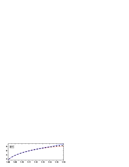
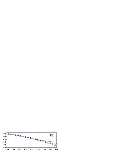
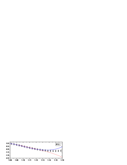
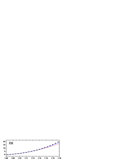
Figure 1: (Color online) Fit up to 1.13 GeV. The fourth- and third-order fits are presented by the solid(blue) and dash(red) lines respectively.

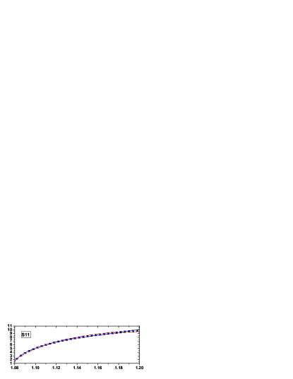
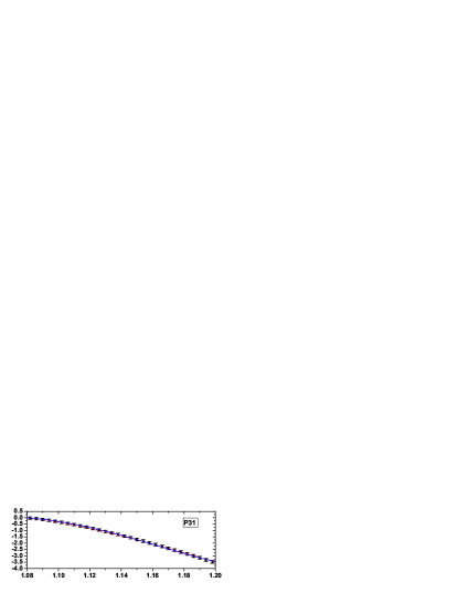
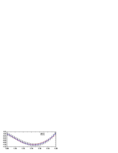
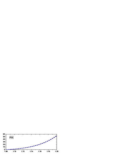
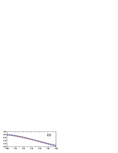
Figure 2: (Color online) Fit up to 1.20 GeV. The fourth- and third-order fits are presented by the solid(blue) and dash(red) lines respectively.

Appendix A Definition of loop integrals

• 1 meson: $\Delta_{\pi}=I_{10}$

  $$\Delta_{\pi}={1\over i}\int{\texttt{d}^{d}k\over(2\pi)^{d}}\frac{1}{M^{2}-k^{2}}.$$

• 1 nucleon: $\Delta_{N}=I_{01}$

  $$\Delta_{N}={1\over i}\int{\texttt{d}^{d}k\over(2\pi)^{d}}\frac{1}{m^{2}-k^{2}}.$$

• 1 meson,1 nucleon:$I=I_{11}$

  $$\{I,I^{\mu},I^{\mu\nu}\}={1\over i}\int{\texttt{d}^{d}k\over(2\pi)^{d}}\frac{\{1,k^{\nu},k^{\mu}k^{\nu}\}}{[M^{2}-k^{2}]\;[m^{2}-(\Sigma-k)^{2}]},$$

  $$I^{\mu}(s)=\Sigma^{\mu}I^{(1)}(s),$$

  $$I^{\mu\nu}(s)=g^{\mu\nu}I^{(2)}(s)+\Sigma^{\mu}\Sigma^{\nu}I^{(3)}(s).$$

• 2 nucleons:$J_{N}=I_{02}$

  $$J_{N}={1\over i}\int{\texttt{d}^{d}k\over(2\pi)^{d}}\frac{1}{[m^{2}-(k-P)^{2}]\;[m^{2}-(k-P^{\prime})^{2}]}.$$

• 1 mesons,2 nucleon:$I_{A}$

  $$I_{A}={1\over i}\int{\texttt{d}^{d}k\over(2\pi)^{d}}\frac{1}{[M^{2}-k^{2}]\;[m^{2}-(P-k)^{2}]\;[m-(P^{\prime}-k)^{2}]}.$$

After removing part proportional to $R=-\frac{1}{\epsilon}+\gamma_{E}-1-\ln 4\pi$, the remaining scalar integrals are finite and denoted by, e.g. $\bar{I}(s)$, $\bar{J}_{N}(t)$, $\bar{I}_{A}(t)$, etc..

References

• [1] J. Gasser, M. E. Sainio and A. Svarc, Nucl. Phys. B 307, 779 (1988).
• [2] E. E. Jenkins and A. V. Manohar, Phys. Lett. B 255, 558 (1991).
• [3] T. Becher and H. Leutwyler, Eur. Phys. J. C 9, 643 (1999)
• [4] T. Fuchs, J. Gegelia, G. Japaridze and S. Scherer, Phys. Rev. D 68, 056005 (2003) .
• [5] L. S. Geng, J. Martin Camalich, L. Alvarez-Ruso and M. J. Vicente Vacas, Phys. Rev. Lett. 101, 222002 (2008)
• [6] N. Fettes, U. -G. Meissner, M. Mojzis and S. Steininger, Annals Phys. 283, 273 (2000) .
• [7] J. M. Alarcon, J. Martin Camalich and J. A. Oller, Prog. Part. Nucl. Phys. 67, 375 (2012) .
• [8] J. M. Alarcon, J. Martin Camalich, J. A. Oller and L. Alvarez-Ruso, Phys. Rev. C 83, 055205 (2011) .
• [9] J. Martin Camalich, J. M. Alarcon and J. A. Oller, Prog. Part. Nucl. Phys. 67, 327 (2012) .
• [10] Y. H. Chen, D. L. Yao, H. Q. Zheng, in preparation.
• [11] R. A. Arndt, W. J. Briscoe, I. I. Strakovsky, R. L. Workman, Phys. Rev. C 74, 045205 (2006) . R. A. Arndt, et al. The SAID program, http://gwdac.phys.gwu.edu.
• [12] V. Pascalutsa and D. R. Phillips, Phys. Rev. C 67, 055202 (2003) .
• [13] N. Fettes and U. -G. Meissner, Nucl. Phys. A 676, 311 (2000).