Critical properties of the Hintermann-Merlini model

Abstract

Many critical properties of the Hintermann-Merlini model are known exactly through the mapping to the eight-vertex model. Wu [J. Phys. C 8, 2262 (1975)] calculated the spontaneous magnetizations of the model on two sublattices by relating them to the conjectured spontaneous magnetization and polarization of the eight-vertex model, respectively. The latter conjecture remains unproved. In this paper, we numerically study the critical properties of the model by means of a finite-size scaling analysis based on transfer matrix calculations and Monte Carlo simulations. All analytic predictions for the model are confirmed by our numerical results. The central charge $c=1$ is found for critical manifold investigated. In addition, some unpredicted geometry properties of the model are studied. Fractal dimensions of the largest Ising clusters on two sublattices are determined. The fractal dimension of the largest Ising cluster on the sublattice A takes fixed value $D_{\rm a}=1.888(2)$, while that for sublattice B varies continuously with the parameters of the model.

I Introduction

The exact solutionsIsing ; YangIsing of the two-dimensional (2D) Ising model significantly promote the research of phase transitions and critical phenomena. After that, the Ising model becomes one of the most famous lattice models in statistical physics. Another famous Ising system, known as the Baxter-Wu modelbw , is defined on the triangular lattice with pure three-spin interactions. The model was firstly proposed by Wood and Griffithswood and exactly solved by Baxter and Wubw by relating the model with the coloring problem on the honeycomb lattice. The solution gives the critical exponents $y_{t}=3/2$ ($\alpha=2/3$) and $y_{h}=15/8$ ($\eta=1/4$), which are exactly the same as those of the 4-state Potts modelpotts ; wfypotts , which can be derived via the Coulomb gas theorydenNijs1 ; denNijs2 ; cg . This means that the Baxter-Wu model belongs to the universality class of the 4-state Potts model. The critical properties of the 4-state Potts model are modified by logarithmic correctionslog2 ; log due to the second temperature field, which is marginally irrelevantNBRS ; log2 . With the two leading temperature fields simultaneously vanishing, the leading critical singularities of the Baxter-Wu modeldengbw do not have logarithmic factors. Deng et al. generalize the Baxter-Wu model in dengbw where the spins are allowed to be $q$ states ($q$ can be larger than 2) and the up- and down-triangles can have different coupling constants. Both generalizations lead to discontinuous phase transitions.

Figure 1: (Color online) Definition of Hintermann-Merlini (HM) model: the lattice consists of two sublattices, the spin on sublattice A is denoted $\sigma$ and the spin on sublattice B is denoted $s$; for a square unit cell, there are four spins $\sigma_{1},\sigma_{2},\sigma_{3}$, and $\sigma_{4}$ on sublattice A and one spin $s$ on sublattice B.

In 1972, Hintermann and Merlinihintermann considered an Ising system on the Union-Jack lattice (as shown in Fig. 1)

$$-\frac{H}{k_{\rm B}T}=\sum\limits_{\Box}s(K_{1}\sigma_{1}\sigma_{2}+K_{2}\sigma_{2}\sigma_{3}+K_{3}\sigma_{3}\sigma_{4}$$

$$+K_{4}\sigma_{4}\sigma_{1}),$$ (1)

where the sum takes over all the square unit cells and $K_{i}$ ($i=1,2,3,4$) are the coupling constants. The model is similar to the Baxter-Wu model in the sense that both are Ising systems with pure three-spin interactions. However the critical properties of the HM model are much more complicated. For the ferromagnetic case ($K_{i}>0$), the model has four-fold degenerate ground states, as shown in Fig. 2. The nature of the phase transition breaking the $Z_{4}$ symmetry of the order parameter cannot be determined by the dimensionality of the system and the symmetry properties of the ground statesSuzuki . The exponents may vary with some tuning parameter without changing the symmetry of the order parameter. Such behavior has been found, e.g., in the Ashkin-Teller model (AT) AT ; ATMC , the eight-vertex model 8vertex ; exactbook , the 2D $XY$ model in a four-fold anisotropic fieldXYh , and the ferromagnetic Ising model with antiferromagnetic next-nearest neighbor couplings on square latticej1j2-henk ; j1j2-sandvik ; j1j2-guo .

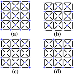
Figure 2: (Color online) Four ground states of the ferromagnetic HM model.

Through mapping to the eight-vertex model8vertex ; exactbook , the free energy of the HM model has been found exactlyhintermann . The critical manifold and critical exponent $y_{t}$ varying with the ratio of couplings were obtained. Based on the conjectured spontaneous magnetization 8v-mag and the spontaneous polarization 8v-polar of the eight-vertex model, Wu calculated the spontaneous magnetizations of the model on two sublattices. The results show that the two magnetizations possess different critical exponentswubw . The spontaneous magnetization of the eight-vertex model was derived later 8v-mag-proof , however, the spontaneous polarization remains a conjecture. It is thus very necessary to verify the results numerically.

In current paper, we study the critical behavior of the ferromagnetic HM model with $K_{1}=K_{3}>0$ and $K_{2}=K_{4}>0$ numerically. The numerical procedure includes transfer matrix calculations and Monte Carlo simulations. The critical properties we studied includes not only the verification of the analytic predictions, but also the fractal structure of spin clusters, which is studied for the first time.

The paper is organized in the following way: In Sec. II, we summarize the theoretical results of the model. In Sec. III, we introduce the transfer matrix method and present the associated numerical results. In Sec. IV, we describe the algorithm used in Monte Carlo simulations and give the associated numerical results. In Sec. V, we define Ising clusters on two sublattices and numerically determine the fractal dimensions of the corresponding largest clusters, respectively. We summarize in Sec. VI.

II Exact solutions

In this section, we summarize the analytical results for the HM modelhintermann ; wubw .

Assign arrows between the nearest-neighboring Ising spins of sublattice A (Fig. 3): if the two spins beside the arrow are the same, the arrow is rightward (or upward), otherwise it is leftward (or downward). There is a two-to-one correspondence between the Ising spin configurations and the arrow configurations.

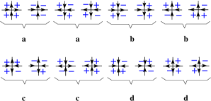
Figure 3: (Color online) The mapping of the HM model to the eight-vertex model and the Boltzmann weights of the vertices. The Ising spins shown here are the spins on sublattice A, namely, the $\sigma$ spins.

After taking sum over the spin $s$ (in the center of the unit cell), the Boltzmann weights of the vertices are

$$a = \cosh(K_{1}+K_{2}+K_{3}+K_{4}),$$

$$b = \cosh(K_{1}-K_{2}+K_{3}-K_{4}),$$

$$c = \cosh(K_{1}-K_{2}-K_{3}+K_{4}),$$

$$d = \cosh(K_{1}+K_{2}-K_{3}-K_{4}).$$ (2)

Thus the model is mapped to the symmetric eight-vertex model8vertex ; exactbook , which has been exactly solved by Baxter. For the ferromagnetic case considered in current paper, the critical manifold is given by

$$a=b+c+d,$$ (3)

which leads to $K_{\rm c}=\log(1+\sqrt{2})/2$ for the uniform case ($K=K_{1}=K_{2}=K_{3}=K_{4}$).

The singularity of the free energy density is governed by

$$f_{\rm sing}\propto|T-T_{\rm c}|^{\pi/u}$$ (4)

when $\pi/2u$ is not an integer (The case that $\pi/2u$ = an integer is not considered in current paper). $T_{\rm c}$ is the critical temperature and $0\leq u\leq\pi$ is given by wubw

$$\cos u = -\tanh[\frac{1}{2}\log\frac{ab}{cd}]\Big{|}_{T_{\rm c}}\quad{\rm if}\ a>b,c,d,$$ (6)

$$~{}~{}~{}~{}~{}~{}~{}~{}~{}~{}~{}~{}~{}~{}~{}~{}~{}~{}~{}~{}~{}~{}~{}~{}~{}~{}~{}~{}~{}{\rm or\ }b>a,c,d$$

$$= \tanh[\frac{1}{2}\log\frac{ab}{cd}]\Big{|}_{T_{\rm c}}\quad\quad{\rm if}\ d>a,b,c,$$

$$~{}~{}~{}~{}~{}~{}~{}~{}~{}~{}~{}~{}~{}~{}~{}~{}~{}~{}~{}~{}~{}~{}~{}~{}~{}~{}~{}~{}~{}{\rm or\ }c>a,b,d.$$

For the ferromagnetic case that we consider, $u$ is determined by (6). Since $f_{\rm sing}\propto\xi^{2}$ and $\xi\sim|T-T_{\rm c}|^{-1/y_{t}}$, the critical exponent $y_{t}$ is thus found

$$y_{t}=\frac{2u}{\pi}.$$ (7)

For the uniform case, (7) gives $y_{t}=4/3$.

A very interesting critical property of the HM model is that the spontaneous magnetizations $M_{\rm A}$ and $M_{\rm B}$ of the sublattice A and B possess different critical exponents:

$$M_{\rm A} \propto (T_{\rm c}-T)^{\beta_{a}},$$

$$M_{\rm B} \propto (T_{\rm c}-T)^{\beta_{b}}.$$ (8)

The critical exponents $\beta_{a}$ and $\beta_{b}$ were obtained by Wuwubw

$${\beta_{a}} = \frac{\pi}{16u},$$

$${\beta_{b}} = \frac{\pi-u}{4u}.$$ (9)

(It should be noted that the author reversely wrote the two critical exponents in Eq. (16) of wubw .) According to the scaling law, this leads to two magnetic exponents $y_{h1}$ and $y_{h2}$

$$y_{h1} =2-\beta_{a}y_{t} =\frac{15}{8},$$

$$y_{h2} =2-\beta_{b}y_{t} =\frac{3\pi+u}{2\pi}.$$ (10)

Here $y_{h1}$ has fixed value $15/8$, while $y_{h2}$ varies continuously with the parameters of the model.

In following sections, we will numerically study the critical properties of the model. The critical points and critical exponents will be numerically verified. Especially, Wu’s result of $\beta_{b}$ ($y_{h2}$) is based on the unproved conjecture of the spontaneous polarization8v-polar of the eight-vertex model, thus numerical verification is very necessary. Our numerical studies are focused on the subspace that $K_{1}=K_{3}=K$ and $K_{2}=K_{4}=K^{\prime}$. By defining $r\equiv K^{\prime}/K$, critical manifold and exponents are expressed as functions of $r$. It is worthy to notice that there is a symmetry for the transformation $r\to 1/r$. At a special point $r^{*}=3.3482581805$ and its dual $1/r^{*}=0.2986627512$, $u=3\pi/4$, the analytic results give $y_{t}=1/2,y_{h1}=15/8=y_{h2}$. This is the 4-state Potts point.

III Transfer matrix calculations

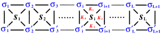
Figure 4: (Color online) Definition of the row-to-row transfer matrix, where periodic boundary conditions are applied, namely $\sigma_{L+1}=\sigma_{1}$, $\sigma_{L+1}^{\prime}=\sigma_{1}^{\prime}$.

As shown in Fig. 4, we define the row-to-row transfer matrix

$$T_{\vec{\sigma},\vec{\sigma}^{\prime}} = \sum\limits_{\{s\}}\prod\limits_{i=1}^{L}\exp[s_{i}(K_{1}\sigma_{i}\sigma_{i+1}+K_{2}\sigma_{i+1}\sigma_{i+1}^{\prime}+$$ (11)

$$K_{3}\sigma_{i+1}^{\prime}\sigma_{i}^{\prime}+K_{4}\sigma_{i}^{\prime}\sigma_{i})]$$

$$= 2^{L}\prod\limits_{i=1}^{L}\cosh(K_{1}\sigma_{i}\sigma_{i+1}+K_{2}\sigma_{i+1}\sigma_{i+1}^{\prime}$$

$$+K_{3}\sigma_{i+1}^{\prime}\sigma_{i}^{\prime}+K_{4}\sigma_{i}^{\prime}\sigma_{i}),$$

where $\vec{\sigma}=(\sigma_{1},\sigma_{2},\cdots,\sigma_{L})$ and $\vec{\sigma}^{\prime}=(\sigma^{\prime}_{1},\sigma^{\prime}_{2},\cdots,\sigma^{\prime}_{L})$ are the states of two neighboring rows, respectively. Here periodic boundary conditions are applied. For a system with $M$ rows, the partition sum is found to be

$$Z = {\rm Trace}(T^{M}),$$ (12)

with the periodic boundary conditions $\vec{\sigma}_{M+1}=\vec{\sigma}_{1}$ applied. In the limit $M\rightarrow\infty$, the free energy density is determined by the leading eigenvalue $\Lambda_{0}$ of $T$

$$f = \frac{1}{L}\log\Lambda_{0}.$$ (13)

For the HM model, the dimension of the matrix $T$ is $d_{T}=2^{L}$. To numerically calculate the eigenvalues of $T$, we used the sparse matrix technique, which sharply reduces the requirement of computer memory for storing the matrix elements. (For details of this technique, see henk1982 ; henk1989 ; henk1993 ; Qian2004 .) We are able to calculate the eigenvalues of $T$ with $L$ up to 22. In our calculations, we restrict the system size $L$ to even values, because the ordered configurations, as shown in Fig. 2, do not fit well in odd systems.

The critical properties can be revealed by calculating three scaled gaps $X_{i}(K,L)$:

$$X_{i}(K,L)=\frac{1}{2\pi}\log\big{(}\frac{\Lambda_{0}}{\Lambda_{i}}\big{)},$$ (14)

where $\Lambda_{i}(i=1,2,3)$ are three subleading eigenvalues of the matrix $T$, respectively. According to the conformal invariance theoryconformal , the scaled gap $X_{i}(K,L)$ is related with a correlation length $\xi_{i}(K,L)$

$$X_{i}(K,L)=\frac{L}{2\pi\xi_{i}(K,L)},$$ (15)

where $\xi_{i}(K,L)$ governs the decay of a correlation function $G_{i}(r)$. According to the finite-size scalingfss , the gap in the vicinity of a critical point scales as

$$X_{i}(K,L) = X_{i}+a_{1}(K-K_{\rm c})L^{y_{t}}+a_{2}(K-K_{c})^{2}L^{2y_{t}}$$ (16)

$$+\cdots+buL^{y_{u}}+\cdots,$$

where $X_{i}$ is the corresponding scaling dimension, which is related to an exponent $y_{i}=2-X_{i}$ according to the conformal invarianceconformal . $u$ is an irrelevant field, and $y_{u}<0$ is the corresponding irrelevant exponent. $a_{1}$,$a_{2}$, and $b$ are unknown constants.

We focus on the the energy-energy correlation $G_{t}(r)$ and two magnetic correlations $G_{A}(r)$ and $G_{B}(r)$. Generally speaking, the magnetic correlation function is defined as $G(r)=\langle s_{0}s_{r}\rangle$. For the HM model, since the spontaneous magnetizations on the two sublattices behave differently, we look two types of magnetic correlation functions: $G_{A}(r)$ with $s_{0}$ and $s_{r}$ on the A sublattice and $G_{B}(r)$ on the B sublattice.

Let $\Lambda_{1}$ be the largest eigenvalue in the subspace that breaks the spin up-down symmetry, which means that the associated eigenvector $\vec{v_{1}}$ satisfies

$$\vec{v_{1}}=-{\mathbf{F}}\vec{v_{1}},$$ (17)

where ${\bf F}$ is the operator flipping spins. Thus, the scaled gap $X_{1}(K,L)$ is identified as $X_{h1}(K,L)$ and the corresponding correlation is $G_{A}(r)$.

Let $\Lambda_{2}$ and $\Lambda_{3}$ be the second and the third largest eigenvalue in the subspace keeping the spin up-down symmetry. It is not a priori clear which of the two corresponding gaps is the thermal one $X_{t}(K,L)$ or the magnetic one $X_{h2}(K,L)$. Based on the magnitudes of $X_{t}=2-y_{t}$ and $X_{h2}=2-y_{h2}$, we identify $X_{2}(K,L)$ and $X_{3}(K,L)$ as $X_{h2}(K,L)$ and $X_{t}(K,L)$, respectively.

Figures 5 and 6 illustrate $X_{h1}(K,L)$ and $X_{h2}(K,L)$ versus $K$ in the uniform case, respectively.

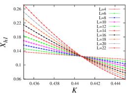
Figure 5: (Color online) Scaled gap $X_{h1}(K,L)$ versus $K$ for a sequence of system size $L$ for the uniform HM model, whose critical point is $K_{\rm c}=\log(1+\sqrt{2})/2=0.440687$.

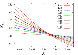
Figure 6: (Color online) Scaled gap $X_{h2}(K,L)$ versus $K$ for a sequence of system size $L$ for the uniform HM model ($r=1$), whose critical point is $K_{\rm c}=\log(1+\sqrt{2})/2=0.440687$.

We then numerically solve the finite-size scaling equation

$$X_{i}(K,L) = X_{i}(K,L-2),$$ (18)

for $i=h1,h2$, respectively. The solution $K_{\rm c}(L)$ satisfies

$$K_{\rm c}(L)=K_{\rm c}+auL^{y_{u}-y_{t}}+\cdots.$$ (19)

Here $a$ is an unknown constant. Since $y_{u}<0$ and $y_{t}\geq 0$, $K_{\rm c}(L)$ converges to the critical point $K_{\rm c}$ with increasing system sizes. (19) is used to determine the critical point in our numerical procedure. For the uniform case, we obtain $K_{\rm c}=0.44068679(5)$, which is in good agreement with the exact solution $K_{\rm c}=\log(1+\sqrt{2})/2$. We have also estimated the critical points of the cases with $r=K^{\prime}/K=2,3,4$, and 5, where $K=K_{1}=K_{3}$ and $K^{\prime}=K_{2}=K_{4}$. Both $X_{h1}(K,L)$ and $X_{h2}(K,L)$ have been used to estimate the critical points, we list the best estimations in Table 1. Our numerical estimations of $K_{\rm c}$ are consistent with the theoretical results in a high accuracy.

Exactly at the critical point $K_{\rm c}$, (16) reduces to

$$X_{i}(K_{\rm c},L) = X_{i}+buL^{y_{u}}+\cdots,$$ (20)

which is used to determine the scaling dimensions $X_{h1}$ and $X_{h2}$. For the uniform case $r=1$, it gives $X_{h1}=0.125000(1)$, and $X_{h2}=0.166666(1)$, which are consistent with the analytic results (Table 1). We applied the same procedure to $r=2,3,4,5$. The numerical estimations and the associated analytic results are consistent, see Table 1.

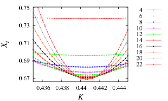
Figure 7: (Color online) Scaled gap $X_{t}(K,L)$ versus $K$ for a sequence of system size $L$ for the uniform HM model ($r=1$), whose critical point is $K_{\rm c}=\log(1+\sqrt{2})/2=0.440687$.

We also calculate the scaled gap $X_{t}(K,L)$ in the vicinity of critical point. The scaling behavior of $X_{t}(K,L)$ seems different from that of $X_{h1}$ or $X_{h2}$, as shown in Fig. 7 for the uniform case. This is the result of $a_{1}=0$ in Eq. (16). The location of the minimum of $X_{t}(K,L)$ for a given $L$ can be denoted as $K_{\rm c}(L)$, which converges to the critical point $K_{\rm c}$ when $L\to\infty$. This property can also be used to estimate $K_{\rm c}$, e.g., as was done in henkcubic . But we don’t do this in current paper. By calculating $X_{t}(K,L)$ at the estimated $K_{\rm c}$, we obtain the scaling dimension $X_{t}$ according to (20). The results are listed in Table 1.

The finite-size-scaling behavior of the free energy density at the critical point determines the central charge $c$ according to fren1 ; fren2

$$f(L)\simeq f(\infty)+\frac{\pi c}{6L^{2}}.$$ (21)

Fitting the data of the free energy density according to (21), we obtain the central charge $c=1.000000(1)$ for the uniform case. For the other cases, the numerical estimations of the central charge are listed in Table 1. The central charge for all $r$ takes the fixed value $c=1$ as expected for transitions breaking four-fold symmetry.

Furthermore, we consider the 4-state Potts point $r=r^{*}=3.3482581805\cdots$. A finite-size scaling analysis based on transfer matrix calculations is performed at this point. The numerical estimations obtained are listed in Table 1. No logarithmic corrections are found, as in the Baxter-Wu model.

Table 1: Critical points, critical exponents, and scaling dimensions of the HM model. $r=K^{\prime}/K$, where $K=K_{1}=K_{3}$ and $K^{\prime}=K_{2}=K_{4}$. $r^{*}=3.3482581805\cdots$. T=Theoretical predictions, MC=Numerical result based on Monte Carlo simulations. TM=Numerical result based on transfer matrix calculations. The critical exponents and the scaling dimensions are related by $y_{t}=2-X_{t}$, $y_{h1}=2-X_{h1}$, and $y_{h2}=2-X_{h2}$.

$r$		1	2	3	$r^{*}$	4	5
$K_{\rm c}$	T	0.4406867935	0.3046889317	0.2406059125	0.225147108	0.2017629641	0.1751991102
	TM	0.44068679(5)	0.3046889(1)	0.2406059(1)	0.2251472(2)	0.2017629(1)	0.1751991(2)
$y_{t}$	T	4/3	1.39668184	1.47604048	3/2	1.53960311	1.58921160
	MC	1.332(2)	1.397(2)	1.478(3)	1.500(1)	1.540(3)	1.590(2)
$X_{t}$	T	2/3	0.60331816	0.52395952	1/2	0.46039689	0.41078840
	TM	0.66666(1)	0.603318(1)	0.52396(1)	0.50000(1)	0.46040(2)	0.41079(1)
$y_{h1}$	T	15/8	15/8	15/8	15/8	15/8	15/8
	MC	1.874(1)	1.874(2)	1.876(2)	1.874(2)	1.877(3)	1.874(2)
$X_{h1}$	T	1/8	1/8	1/8	1/8	1/8	1/8
	TM	0.125000(1)	0.125000(1)	0.125000(1)	0.12499(1)	0.12500(1)	0.12498(3)
$y_{h2}$	T	11/6	1.84917046	1.86901012	15/8	1.88490078	1.89730290
	MC	1.833(1)	1.848(2)	1.870(2)	1.875(1)	1.886(2)	1.896(4)
$X_{h2}$	T	1/6	0.15082954	0.13098988	1/8	0.11509922	0.10269710
	TM	0.166666(1)	0.150829(1)	0.130990(1)	0.12500(1)	0.115099(1)	0.102696(2)
$c$	T	1	1	1	1	1	1
	MC	1.000000(1)	1.000000(1)	0.99998(3)	1.0000(1)	1.0000(2)	0.9999(1)

IV Monte Carlo simulations

The Baxter-Wu model has been simulated by the Metropolis algorithmbwMC , the Wang Landau algorithmwanglandau , and a cluster algorithmhenkbw ; dengbw . The cluster algorithm is similar to the Swendsen-Wang algorithmsw for the Potts model. In this algorithm, the triangular lattice is divided as three triangular sublattices. By randomly freezing the spins on one of the sublattices, the other two sublattices compose a honeycomb lattice with pair interactions, then a Swendsen-Wang type algorithm can be formed to update the spins on this honeycomb lattice. In current paper, we suitably modify this cluster algorithm to simulate the HM model.

The algorithm is divided into three steps:

1. Step 1, update the spins on sublattice A.

   Let the spins on sublattice B be unchanged (frozen), the interactions of the spins reduce to pair interactions on sublattice A.

   A. bonds. An vertical (horizontal) edge on sublattice A belongs to two triangles, the interactions of the left (upper) and right (down) triangles can be denoted $K_{l}$ and $K_{r}$ respectively, which may take the values $K_{1},K_{2},K_{3}$, or $K_{4}$. Place a bond on this edge with probability $p=1-e^{-2K_{l}-2K_{r}}$ if both the products of spins in the left (upper) triangle and in the right (down) triangle are 1, $p=1-e^{-2K_{l}}$ if only the product in the left (upper) triangle is 1, $p=1-e^{-2K_{r}}$ if only the product in the right (down) triangle is 1, $p=0$ otherwise.

   B. clusters. A cluster is defined as a group of sites on sublattice A connected through the bonds.

   C. update spins. Independently flip the spins of each cluster with probability 1/2.

2. Step 2, update the spins on sublattice B and half of the spins on sublattice A.

   This step is very similar to step 1, but we freeze only half of the spins on sublattice A, which are labeled ${\rm A_{1}}$ (Fig. 8). The other spins (on sublattice B+${\rm A_{2}}$) are updated, whose interactions also reduce to pair interactions when ${\rm A_{1}}$ spins are frozen.

3. Step 3, update the spins on sublattice B and the other half of the spins on sublattice A.

   In this step, the spins labeled ${\rm A_{2}}$ (in Fig. 8) are frozen, other spins (on sublattice B+${\rm A_{1}}$) are updated.

In a complete sweep, all the spins are updated twice.

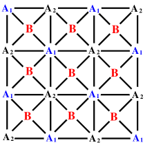
Figure 8: (Color online) When ${\rm B}$ spins are frozen, the interactions of ${\rm A}$ spins (${\rm A_{1}}$ and ${\rm A_{2}}$ spins) reduce to pair interactions; when ${\rm A_{1}}$ spins are frozen, the interactions of ${\rm B+A_{2}}$ spins reduce to pair interactions; when ${\rm A_{2}}$ spins are frozen, the interactions of ${\rm B+A_{1}}$ spins reduce to pair interactions.

In the simulations, the sampled variables include the specific heat $C$, the magnetizations $M_{\rm A}$ on sublattice A, and $M_{\rm B}$ on sublattice B.

The specific heat is calculated from the fluctuation of energy density $E$

$$C=\frac{L^{2}(\langle E^{2}\rangle-\langle E\rangle^{2})}{k_{B}T^{2}},$$ (22)

where $L$ is the linear size of the system, and $\langle\cdots\rangle$ means the ensemble average. The magnetizations are defined as

$$M_{\rm A} = \frac{\big{\langle}\big{|}\sum\limits_{i=1}^{N}\sigma_{i}\big{|}\big{\rangle}}{N},$$ (23)

$$M_{\rm B} = \frac{\big{\langle}\big{|}\sum\limits_{i=1}^{N}s_{i}\big{|}\big{\rangle}}{N},$$ (24)

where $N=L^{2}$ is the number of total sites on sublattice A or B.

In order to demonstrate our numerical procedure based on the Monte Carlo simulations, we take the uniform case ($K=K_{1}=K_{2}=K_{3}=K_{4}$) as an example. The cluster algorithm is very efficient, which easily allows us to do meaningful simulations for system with linear size up to $L=384$. All the simulations are performed at the critical point $K_{\rm c}$. After equilibrating the system, $10^{7}$ samples were taken for each system size. Using the Levenberg-Marquardt algorithm, we fit the data of $C$ according to the finite-size scaling formulafss

$$C(L)=C_{0}+L^{2y_{t}-d}(a+bL^{y_{1}}),$$ (25)

where $bL^{y_{1}}$ are the leading correction-to-scaling term with $y_{1}<0$ the leading irrelevant exponent. $d=2$ is the dimensionality of the lattice. $C_{0}$, $a$, and $b$ are unknown parameters. The fitting yields $y_{t}=1.332(2)$, which is in good agreement with the exact result $y_{t}=4/3$.

The finite-size scaling behaviors of the magnetizations $M_{\rm A}$ and $M_{\rm B}$ are

$$M_{\rm A} = L^{y_{h1}-d}(a+bL^{y_{1}}),$$ (26)

$$M_{\rm B} = L^{y_{h2}-d}(a^{\prime}+b^{\prime}L^{y^{\prime}_{1}}),$$ (27)

respectively. The log-log plot of $M_{\rm A}$ and $M_{\rm B}$ versus $L$ are shown in Fig. 9. The fits yield $y_{h1}=1.874(1)$, and $y_{h2}=1.833(1)$, where $y_{h1}$ and $y_{h2}$ are in good agreement with the analytic predictions $y_{h1}=15/8$ and $y_{h2}=11/6$, respectively.

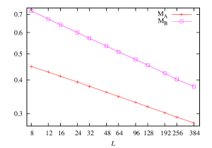
Figure 9: (Color online) Log-Log plot of the magnetizations $M_{\rm A}$ and $M_{\rm B}$ versus system size $L$ for the HM model at the critical point $K_{\rm c}=\log(1+\sqrt{2})/2$ for the uniform case ($K=K_{1}=K_{2}=K_{3}=K_{4}$).

We also simulate the $r=2,3,4,5$, and $r^{*}$ cases. The numerical estimations of $y_{t},y_{h1},y_{h2}$ and the corresponding analytic predictions are listed in Table 1. They are in good agreement. In these fits, no logarithmic corrections to scaling are found.

V Fractal structure of the model

In addition to calculate the critical exponents $y_{t}$, $y_{h1}$, and $y_{h2}$, we also investigate the geometry properties of the model.

The configurations of the HM model are represented by Ising spins. Thus we can define “Ising clusters” for the model as in the Ising modelIsingCluster . To do so, each sublattice is viewed as a square lattice. For two nearest-neighboring Ising spins on a sublattice, they are considered to be in the same cluster if they have the same sign. Here, in saying “nearest-neighboring”, the neighborhood of the site is the same to that of a site in a square lattice. This definition is applied to the two sublattices respectively, thus there are two types of Ising clusters. For clarity, we call the Ising cluster on sublattice A as “A cluster”, while the Ising cluster on sublattice B as “B cluster”.

The simulations are also performed at the critical points. The size of the largest A cluster and the largest B cluster are denoted $S_{a}$ and $S_{b}$, respectively. They satisfy the finite-size scaling

$$S_{a} = L^{D_{a}}(a+bL^{y_{1}}),$$ (28)

$$S_{b} = L^{D_{b}}(a^{\prime}+b^{\prime}L^{y^{\prime}_{1}}),$$ (29)

which means that the largest A cluster and the largest B cluster are fractals, with $D_{a}$ and $D_{b}$ the fractal dimensions, respectively. Figure 10 is an illustration of $S_{a}$ and $S_{b}$ versus system size $L$ at the uniform case. Fitting the data according to (28) and (29), we find $D_{a}=1.888(1)$ and $D_{b}=1.925(1)$.

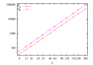
Figure 10: (Color online) Log-Log plot of $S_{a}$ and $S_{b}$ versus system size $L$ for the HM model at the critical point $K_{\rm c}=\log(1+\sqrt{2})/2$ for the uniform case ($K=K_{1}=K_{2}=K_{3}=K_{4}$).

The same procedure were applied to $r=2,3,4,5$ and $r^{*}$. The results obtained are listed in Table. 2. The fractal dimension of the A cluster has a fixed value $D_{a}=1.888(2)$, while that of the B cluster varies with the ratio $r$.

Table 2: Fractal dimensions of the HM model. $D_{a}$ is the fractal dimension of A cluster, $D_{b}$ is the fractal dimension of B cluster. $r=K^{\prime}/K$, where $K=K_{1}=K_{3}$ and $K^{\prime}=K_{2}=K_{4}$, $r^{*}=3.3482581805$.

$r$	1	2	3	$r^{*}$	4	5
$D_{a}$	1.888(1)	1.889(1)	1.890(3)	1.889(2)	1.888(1)	1.888(2)
$D_{b}$	1.925(1)	1.931(1)	1.939(1)	1.941(1)	1.945(2)	1.951(2)

VI Conclusion and discussions

In conclusion, we have numerically studied the critical properties of the HM model by means of finite-size scaling analysis based on the transfer matrix calculations and the Monte Carlo simulations. For the critical points and the critical exponents $y_{t}$ ($X_{t}$), $y_{h1}$ ($X_{h1}$), and $y_{h2}$ ($X_{h2}$), our numerical estimations are in good agreement with the corresponding analytic predictionshintermann ; wubw . The analytic prediction for $y_{h2}$ is based on the conjectured spontaneous polarization of the eight-vertex model, which remains unproved. Our numerical results verified the correctness of the prediction.

In addition the central charge of the model is found to be $c=1$. This is consistent with the fact that $y_{h1}=15/8$, $y_{t}$ and $y_{h2}$ vary continuously with the parameters, which is related to the four-fold degeneracy of the ground states of the model. Usually, logarithmic correctionslog ; lvAT ; j1j2-guo show up in the 4-state Potts point for the model with 4-fold degenerate ground states due to the second temperature field. However, we do not see such logarithmic corrections in the 4-state Potts point of the HM model. This is the same as the Baxter–Wu model, in which the amplitude of the marginally irrelevant operator is zero.

Furthermore, two unpredicted critical exponents are found to describing geometry properties of the model. We define clusters based on the Ising-spin configurations on the two sublattices of the model. The fractal dimension of the largest cluster on sublattice A takes fixed value $D_{a}=1.888(2)$, while the fractal dimension of the largest cluster on sublattice B varies continuously with the parameter of the model.

References

- (1) L. Onsager, Phys. Rev. 65, 117 (1944).
- (2) C. N. Yang, Phys. Rev. 85, 808 (1952).
- (3) R. J. Baxter and F. Y. Wu, Phys. Rev. Lett. 31, 1294 (1973).
- (4) D. W. Wood and H. P. Griffiths, J. Phys. C 5, L253 (1972).
- (5) R. B. Potts, Proc. Camb. Phys. Soc. 48, 106 (1952).
- (6) F. Y. Wu, Rev. Mod. Phys. 54, 235 (1982).
- (7) M. P. M. den Nijs, J. Phys. A 12, 1857 (1979).
- (8) M. P. M. den Nijs, Phys. Rev. B 27, 1674 (1983).
- (9) B. Nienhuis, J. Stat. Phys. 34, 731 (1984).
- (10) B. Nienhuis, A. N. Berker, E. K. Riedel, M. Schick, Phys. Rev. Lett. 43, 737 (1979).
- (11) J. Salas and A. D. Sokal, J. Stat. Phys. 88, 567 (1997).
- (12) M. Nauenberg, D. J. Scalapino, Phys. Rev. Lett. 44, 837 (1980).
- (13) Y. Deng, W.-A. Guo, J. R. Heringa, H. W. J. Blöte, and B. Neinhuis, Nucl. Phys. B 827[FS], 406 (2010).
- (14) A. Hintermann and D. Merlini, Phys. Lett. A, 41, 208 (1972).
- (15) M. Suzuki, Prog. Theor. Phys. 51, 1992 (1974).
- (16) J. Ashkin and E. Teller, Phys. Rev. 64, 178 (1943).
- (17) S. Wiseman and E. Domany, Phys. Rev. E 48, 4080 (1993).
- (18) J.-P. Lv, Y. Deng, and Q.-H. Chen, Phys. Rev. E 84, 021125(2011).
- (19) M. P. Nightingale and H. W. J. Blöte, Physica A 251, 211 (1998).
- (20) S. Jin, A. Sen, and A. W. Sandvik, Phys. Rev. Lett. 108, 045702 (2012).
- (21) S. Jin, A. Sen, W.-A. Guo, and A. W. Sandvik, Phys. Rev. B 87, 144406(2013).
- (22) R. J. Baxter, Phys. Rev. Lett. 26, 832 (1971).
- (23) R. J. Baxter, Exactly Solved Models in Statistical Mechanics (Academic, London, 1982).
- (24) J. V. José, L. P. Kadanoff, S. Kirkpatrick, and D. R. Nelson, Phys. Rev. B 16, 1217 (1977).
- (25) M. N. Barber and R. J. Baxter, J. Phys. C 6, 2913 (1973).
- (26) R. J. Baxter and S. B. Kelland, J. Phys. C 7, L403 (1974).
- (27) F. Y. Wu, J. Phys. C 8, 2262 (1975).
- (28) R. J. Baxter, J. Stat. Phys. 15, 485 (1976).
- (29) H. W. J. Blöte and M. P. Nightingale, Physica A (Amsterdam) 112, 405 (1982).
- (30) H. W. J. Blöte and B. Nienhuis, J. Phys. A 22, 1415 (1989).
- (31) H. W. J. Blöte and M. P. Nightingale, Phys. Rev. B 47, 15046 (1993).
- (32) X. F. Qian, M. Wegewijs, and H. W. J. Blöte, Phys. Rev. E 69, 036127 (2004).
- (33) J. L. Cardy, in Phase Transitions and Critical Phenomena, edited by C. Domb and J. L. Lebowitz (Academic Press, London, 1987), Vol. 11, p. 55, and references therein.
- (34) For reviews, see e.g. M. P. Nightingale in Finite-Size Scaling and Numerical Simulation of Statistical Systems, ed. V. Privman (World Scientific, Singapore 1990), and M. N. Barber in Phase Transitions and Critical Phenomena, Vol. 8, eds. C. Domb and J. L. Lebowitz (Academic, New York, 1983).
- (35) H. W. J. Blöte, M. P. Nightingale, Physica A (Amsterdam) 129, 1 (1984).
- (36) H. W. J. Blöte, J. L. Cardy, and M. P. Nightingale, Phys. Rev. Lett. 56, 742 (1986).
- (37) I. Affleck, Phys. Rev. Lett. 56, 746 (1986).
- (38) L. N. Shchur and W. Janke, arXiv:1007.1838.
- (39) N. Schreiber and J. Adler, J .Phys. A 38, 7253 (2005).
- (40) H. W. J. Blöte, J. R. Heringa, and E. Luijten, Comp. Phys. Comm. 147, 58 (2002).
- (41) R. H. Swendsen and J. S. Wang, Phys. Rev. Lett. 58, 86 (1987).
- (42) W. Janke and A. M. J. Schakel, Phys. Rev. E 71, 036703 (2005).