A Calculus of Looping Sequences with Local Rules

Abstract

In this paper we present a variant of the Calculus of Looping Sequences (CLS for short) with global and local rewrite rules. While global rules, as in CLS, are applied anywhere in a given term, local rules can only be applied in the compartment on which they are defined. Local rules are dynamic: they can be added, moved and erased. We enrich the new calculus with a parallel semantics where a reduction step is lead by any number of global and local rules that could be performed in parallel. A type system is developed to enforce the property that a compartment must contain only local rules with specific features. As a running example we model some interactions happening in a cell starting from its nucleus and moving towards its mitochondria.

1 Introduction

The Calculus of Looping Sequences (CLS for short) [6, 5, 16, 7], is a formalism for describing biological systems and their evolution. CLS is based on term rewriting with a set of predefined rules modelling the activities one would like to describe. CLS terms are constructed by starting from a set of basic constituent elements which are composed with operators of sequencing, looping, containment and parallel composition. Sequences may represent DNA fragments and proteins, looping sequences may represent membranes, parallel composition may represent juxtaposition of elements and populations of chemical species.

The model has been extended with several features such as bisimulations [5, 8], combining the simplicity of notation of rewrite systems with the advantage of a form of compositionality. In [2, 3] a type system was defined to ensure the well-formedness of links between protein sites within the Linked Calculus of Looping Sequences (see [4]). In [14] we defined a type system to guarantee the soundness of reduction rules with respect to the requirement of certain elements, and the repellency of others.

In this paper we present a variant of CLS with global and local rewrite rules (CLSLR, for short). Global rules are applied anywhere in a given term wherever their patterns match the portion of the system under investigation, local rules can only be applied in the compartment in which they are defined. Terms written in CLSLR are thus syntactically extended to contain explicit local rules within the term, on different compartments. Local rules can be created, moved between different compartments and deleted. We feel that having a calculus in which we can model the dynamic evolution of the rules describing the system results in a more natural and direct way to study emerging properties of complex systems. As it happens in nature, where data and programs are encoded in the same kind of molecular structures, we insert rewrite rules within the terms modelling the system under investigation.

In CLSLR we also enrich CLS with a parallel semantics in which we define a reduction step lead by any number of global and local rules that could be performed in parallel.

Since in this framework the focus is put on local rules, we define a set of features that can be associated to each local rule. Features may define general properties of rewrite rules or properties which are strictly related to the model under investigation. We define a membrane type for the compartments of our model and develop a type systems enforcing the property that a compartment must contain only local rules with specific features.

Thus, the main features of CLSLR are:

• different compartments can evolve according to different local rules;

• the set of global rules is fixed;

• local rules are dynamic: they can be added, moved and erased according to both global and local rules;

• a parallel reduction step permits the application of several global and local rules;

• compartments are enforced to contain only rules with specific features.

As a running case study, emphasising the peculiarities of the calculus, we consider some mitochondrial activity underlining the form of symbiosis between a cell and its mitochondria (see [15]). Mitochondria are membrane-enclosed organelle found in eukaryotic cells that generate most of the cell’s energy supply in the form of adenosine triphosphate (ATP). A mitochondrion is formed by two membranes, the outer and the inner membrane, having different properties and proteins on their surfaces. Both membranes have receptors to mediate the entrance of molecules. In Figure 1 we show the expression of a gene (encoded in the DNA within the nucleus of the cell) destined to be translated into a protein that will be catch by mitochondria and will then catalyse the production of ATP. In particular, we will model the following steps: (1) genes within the nucleus’ DNA are transcribed into mRNA, (2) mRNA moves from the nucleus to the cell’s cytoplasm, (3) where it is translated into the protein.

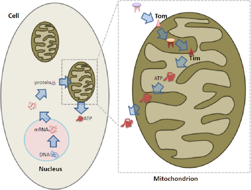
Figure 1: From the cell nucleus to mitochondria.

The vast majority of proteins destined for the mitochondria are encoded in the nucleus of the cell and synthesised in the cytoplasm. These are tagged by a signal sequence, which is recognised by a receptor protein in the Transporter Outer Membrane complex (TOM). The signal sequence and adjacent portions of the polypeptide chain are inserted in the intermembranous space through the TOM complex, then in the mitochondrion internal space through a Transporter Inner Membrane complex (TIM). According to this description, we model the following final steps: (4) protein is detected by TOM and brought within the intermembranous space, (5) then, through TIM, in the mitochondrion’s inside, (6) where it catalyses the production of ATP, (7) that exits the inner, (8) and the outer mitochondrial membranes towards the cell’s cytoplasm.

2 The calculus

In this Section we present the Calculus of Looping Sequences with Local Rules (CLSLR).

2.1 Syntax of CLSLR

We assume a possibly infinite alphabet $\mathcal{E}$ of symbols ranged over by $a,b,c,\ldots$, a set of element variables $\mathcal{X}$ ranged over by $x,y,z,\ldots$, a set of sequence variables $\mathcal{SV}$ ranged over by $\widetilde{x},\widetilde{y},\widetilde{z},\ldots$, and a set of term variables $\mathcal{TV}$ ranged over by $X,Y,Z,\ldots$. All these sets are possibly infinite and pairwise disjoint. We denote by $\mathcal{V}$ the set of all variables, $\mathcal{V}=\mathcal{X}\cup\mathcal{SV}\cup\mathcal{TV}$, and with $\chi$ a generic variable of $\mathcal{V}$. Hence, a pattern is a term that may include variables.

Definition 2.1.

[Patterns] Patterns $P$, sequence patterns $SP$ and local rules $R$ of CLS are given by the following grammar:

$$\begin{array}[]{lll}P&\mathrel{\makebox[20.00003pt]{$::=$}}&\left(SP\right)^{\circlearrowleft}\,\rfloor\,P\quad\big{|}\quad P\;|\;P\quad\big{|}\quad L\\ SP&\mathrel{\makebox[20.00003pt]{$::=$}}&\epsilon\quad\big{|}\quad a\quad\big{|}\quad x\quad\big{|}\quad SP\cdot SP\quad\big{|}\quad\widetilde{x}\\ L&\mathrel{\makebox[20.00003pt]{$::=$}}&X\quad\big{|}\quad SP\quad\big{|}\quad L\;|\;L\quad\big{|}\quad R\\ R&\mathrel{\makebox[20.00003pt]{$::=$}}&L\!\mapsto\!L\quad\big{|}\quad L^{\uparrow SP}\!\mapsto\!L^{\uparrow SP}\quad\big{|}\quad L^{\downarrow SP}\!\mapsto\!L^{\downarrow SP}\end{array}$$

where $a$ is a generic element of $\mathcal{E}$, and $X,\widetilde{x}$ and $x$ are generic elements of $\mathcal{TV},\mathcal{SV}$ and $\mathcal{X}$, respectively. Sequence patterns $SP$ defines patterns for sequences of elements, $\left(SP\right)^{\circlearrowleft}$ denotes a closed (looping) sequence which may contain other patterns through the $\,\rfloor\,$ operator, $\;|\;$ is used to denote the parallel composition (juxtaposition) of patterns, and $R$ denotes the syntax of local rules that may either exit ($L^{\uparrow SP}$) or enter ($L^{\downarrow SP}$) a closed sequence $SP$. We denote with $\mathcal{P}$ the infinite set of patterns.
A local rule $L_{1}\!\mapsto\!L_{2}$ is well formed if $L_{1}\not\equiv\epsilon$ and $Var(L_{2})\subseteq Var(L_{1})$, where $Var(P)$ denotes set of variables appearing in $P$.
A local rule $L_{1}^{\uparrow SP_{1}}\!\mapsto\!L_{2}^{\uparrow SP_{2}}$ or $L_{1}^{\downarrow SP_{1}}\!\mapsto\!L_{2}^{\downarrow SP_{2}}$ is well formed if $L_{1}\not\equiv\epsilon$, $Var(L_{2})\subseteq Var(L_{1})$ and $Var(SP_{2})\subseteq Var(SP_{1})$.

Terms are patterns containing variables only inside local rules. Sequences are closed sequence patterns. We denote with $\mathcal{T}$ the infinite set of terms, ranged over by $T$, and with $\mathcal{S}$ the infinite set of sequences, ranged over by $S$.

An instantiation is a partial function $\sigma:(\mathcal{TV}\rightarrow\mathcal{T})\cup(\mathcal{SV}\rightarrow\mathcal{S})\cup(\mathcal{X}\rightarrow\mathcal{E})$. Given $P\in\mathcal{P}$, with $P\sigma$ we denote the term obtained by replacing each occurrence of each variable $\chi\in\mathcal{V}$ appearing in $P$ with the corresponding term $\sigma(\chi)$, but for local rules, which are left unchanged by instantiations, i.e., $R\sigma=R$ for all $R$ and $\sigma$. With $\Sigma$ we denote the set of all the possible instantiations.

Definition 2.2 (Structural Congruence).

The structural congruence relations $\equiv_{S}$ and $\equiv_{R}$ and $\equiv_{P}$ are the least congruence relations on sequence patterns, local rules and on patterns, respectively, satisfying the rules shown in Figure 2.

$$\begin{array}[]{c}SP_{1}\cdot(SP_{2}\cdot SP_{3})\equiv_{S}(SP_{1}\cdot SP_{2})\cdot SP_{3}\qquad SP\cdot\epsilon\equiv_{S}\epsilon\cdot SP\equiv_{S}SP\\ SP_{1}\equiv_{S}SP_{2}\ \mbox{ implies }\ SP_{1}\equiv_{P}SP_{2}\ \mbox{ and }\ \left(SP_{1}\right)^{\circlearrowleft}\,\rfloor\,P\equiv_{P}\left(SP_{2}\right)^{\circlearrowleft}\,\rfloor\,P\\ L_{1}\equiv_{P}L^{\prime}_{1}\ \mbox{ and }L_{2}\equiv_{P}L^{\prime}_{2}\ \mbox{ imply }L_{1}\!\mapsto\!L_{2}\equiv_{R}L^{\prime}_{1}\!\mapsto\!L^{\prime}_{2}\\ L_{1}\equiv_{P}{L^{\prime}}_{1}\ \mbox{ and }L_{2}\equiv_{P}{L^{\prime}}_{2}\ \mbox{ and }\ \ SP_{1}\equiv_{P}{SP^{\prime}}_{1}\ \mbox{ and }\ \ SP_{2}\equiv_{P}{SP^{\prime}}_{2}\\ \mbox{ imply }L_{1}^{\uparrow SP_{1}}\!\mapsto\!L_{2}^{\uparrow SP_{2}}\equiv_{R}{L^{\prime}}_{1}^{\uparrow{SP^{\prime}}_{1}}\!\mapsto\!{L^{\prime}}_{2}^{\uparrow{SP^{\prime}}_{2}}\ \mbox{ and }\ L_{1}^{\downarrow SP_{1}}\!\mapsto\!L_{2}^{\downarrow SP_{2}}\equiv_{R}{L^{\prime}}_{1}^{\downarrow{SP^{\prime}}_{1}}\!\mapsto\!{L^{\prime}}_{2}^{\downarrow{SP^{\prime}}_{2}}\\ R_{1}\equiv_{R}R_{2}\ \mbox{ implies }\ R_{1}\equiv_{P}R_{2}\\ P_{1}\;|\;P_{2}\equiv_{P}P_{2}\;|\;P_{1}\qquad P_{1}\;|\;(P_{2}\;|\;P_{3})\equiv_{P}(P_{1}\;|\;P_{2})\;|\;P_{3}\qquad P\;|\;\epsilon\equiv_{P}P\\ \left(\epsilon\right)^{\circlearrowleft}\,\rfloor\,\epsilon\equiv_{P}\epsilon\qquad\left(SP_{1}\cdot SP_{2}\right)^{\circlearrowleft}\,\rfloor\,P\equiv_{P}\left(SP_{2}\cdot SP_{1}\right)^{\circlearrowleft}\,\rfloor\,P\end{array}$$

Figure 2: Structural Congruence

Structural congruence rules the state the associativity of $\cdot$ and $\;|\;$, the commutativity of the latter and the neutral role of $\epsilon$. Moreover, axiom $\left(SP_{1}\cdot SP_{2}\right)^{\circlearrowleft}\,\rfloor\,P\equiv_{P}\left(SP_{2}\cdot SP_{1}\right)^{\circlearrowleft}\,\rfloor\,P$ says that looping sequences can rotate. In the following, for simplicity, we will use $\equiv$ in place of $\equiv_{P}$.

2.2 (Parallel) Operational Semantics

In order to define a reduction step in which (possibly) more than one rule is applied, following [11], we first define the application of a single rule, either global or local. We resort to the standard notion of evaluation contexts.

Definition 2.3 (Contexts).

Evaluation Contexts $E$ are defined as:

$$E::=\square\quad\big{|}\quad E\;|\;T\quad\big{|}\quad T\;|\;E\quad\big{|}\quad\left(S\right)^{\circlearrowleft}\,\rfloor\,E$$

where $T\in\mathcal{T}$ and $S\in\mathcal{S}$. The context $\square$ is called the empty context. We denote with $E\!\!\!\!\!E$ the infinite set of evaluation contexts.

By definition, every evaluation context contains a single hole $\square$. Let us assume $E\in E\!\!\!\!\!E$, with $E[T]$ we denote the term obtained by replacing $\square$ with $T$ in $E$. The structural equivalence is extended to contexts in the natural way (by considering $\square$ as a new and unique symbol of the alphabet $\mathcal{E}$). Note that the shape of evaluation contexts does not permit to have holes in sequences. A rewrite rule introducing a parallel composition on the right hand side (as $a\mapsto b\;|\;c$) applied to an element of a sequence (e.g., $m\!\cdot\!a\!\cdot\!m$) would result into a syntactically incorrect term (in this case $m\cdot(b\;|\;c)\cdot m$).

To enforce the fact that local and global rule applications can be done in parallel, we underline those subterms that are produced by the application of the rule involved. Terms matching the left-hand-side of a (local or global) rule must not have any underlined subterm. Underlined terms are only used for bookkeeping in the definition of rule application.

Let $\underline{\mathcal{T}}$ denote the set of terms in which some subterms can be underlined. The erasing mapping $\eta:\underline{\mathcal{T}}\mapsto\mathcal{T}$ erases all underlining obtaining a term generated by the grammar of Definition 2.1.

We first define the application of global or local rules to terms in $\underline{\mathcal{T}}$ which produces terms in $\underline{\mathcal{T}}$.

Global rules are of the shape $P_{1}\mapsto P_{2}$. They can be applied to terms only if they occur in a legal evaluation context.

Local rules are inside compartments, and can be applied only if a term matching the left-hand-side of the rule occurs in the same compartment.

Notice that global rules have patterns $P$ on both the left and the right-hand side of the rules, whereas local rules have the less general $L$ patterns. In particular, $L$ patterns do not contain compartments, and therefore cannot change the nesting structure of the compartments of a term.

Definition 2.4 (Rule Application).

Given a finite set of global rules $\mathcal{R}$, the rule application $\xrightarrow{}$ is the least relation closed with respect to $\equiv$ defined by:

$${tensy\vbox{\hbox spread0.0pt{\hskip 0.0pt plus 0.0001fil\hbox{$\displaystyle\penalty 1\begin{array}[]{c}P_{1}\mapsto P_{2}\in\mathcal{R}\quad\sigma\in\Sigma\quad P_{1}\sigma\not\equiv\epsilon\end{array}$}\hskip 0.0pt plus 0.0001fil}\hbox{\hbox{\kern 0.0pt\vrule height=0.25002pt,depth=0.25002pt,width=120.50897pt\hbox{\kern 3.00003pt$\scriptstyle{\textsc{(GRT)}}$}}}\hbox{\kern 33.57901pt\hbox{$\displaystyle E[P_{1}\sigma]\xrightarrow{}E[\underline{P_{2}\sigma}]$}}}}$$

$${tensy\vbox{\hbox spread0.0pt{\hskip 0.0pt plus 0.0001fil\hbox{\kern 43.82057pt\hbox{$\displaystyle\penalty 1\begin{array}[]{c}\sigma\in\Sigma\quad L_{1}\sigma\not\equiv\epsilon\end{array}$}}\hskip 0.0pt plus 0.0001fil}\hbox{\hbox{\kern 0.0pt\vrule height=0.25002pt,depth=0.25002pt,width=161.90074pt\hbox{\kern 3.00003pt$\scriptstyle{\textsc{(LR)}}$}}}\hbox{\kern 0.0pt\hbox{$\displaystyle E[L_{1}\mapsto L_{2}\;|\;L_{1}\sigma\;|\;T]\xrightarrow{}E[L_{1}\mapsto L_{2}\;|\;\underline{L_{2}\sigma}\;|\;T]$}}}}$$

$${tensy\vbox{\hbox spread0.0pt{\hskip 0.0pt plus 0.0001fil\hbox{\kern 81.62065pt\hbox{$\displaystyle\penalty 1\begin{array}[]{c}\sigma\in\Sigma\quad L_{1}\sigma\not\equiv\epsilon\end{array}$}}\hskip 0.0pt plus 0.0001fil}\hbox{\hbox{\kern 0.0pt\vrule height=0.25002pt,depth=0.25002pt,width=237.5009pt\hbox{\kern 3.00003pt$\scriptstyle{\textsc{(LR-Out)}}$}}}\hbox{\kern 0.0pt\hbox{$\displaystyle E[\left(S_{1}\sigma\right)^{\circlearrowleft}\,\rfloor\,(L_{1}^{\uparrow S_{1}}\mapsto L_{2}^{\uparrow S_{2}}\;|\;L_{1}\sigma\;|\;T)]\xrightarrow{}E[\underline{L_{2}\sigma}\;|\;\left(\underline{S_{2}\sigma}\right)^{\circlearrowleft}\,\rfloor\,(L_{1}^{\uparrow S_{1}}\mapsto L_{2}^{\uparrow S_{2}}\;|\;T)]$}}}}$$

$${tensy\vbox{\hbox spread0.0pt{\hskip 0.0pt plus 0.0001fil\hbox{\kern 77.73175pt\hbox{$\displaystyle\penalty 1\begin{array}[]{c}\sigma\in\Sigma\quad L_{1}\sigma\not\equiv\epsilon\end{array}$}}\hskip 0.0pt plus 0.0001fil}\hbox{\hbox{\kern 0.0pt\vrule height=0.25002pt,depth=0.25002pt,width=229.7231pt\hbox{\kern 3.00003pt$\scriptstyle{\textsc{(LR-In)}}$}}}\hbox{\kern 0.0pt\hbox{$\displaystyle E[L_{1}^{\downarrow S_{1}}\mapsto L_{2}^{\downarrow S_{2}}\;|\;L_{1}\sigma\;|\;\left(S_{1}\sigma\right)^{\circlearrowleft}\,\rfloor\,T]\xrightarrow{}E[L_{1}^{\downarrow S_{1}}\mapsto L_{2}^{\downarrow S_{2}}\;|\;\left(\underline{S_{2}\sigma}\right)^{\circlearrowleft}\,\rfloor\,(T\;|\;\underline{L_{2}\sigma})]$}}}}$$

With rule (LR-Out) a term or a rule $L_{1}\sigma$ exits from the membrane in which it is contained only if the membrane has as loop the sequence $S_{1}\sigma$: when outside, $L_{1}\sigma$ is transformed into $L_{2}\sigma$, and the sequence $S_{1}\sigma$ into $S_{2}\sigma$. (LR-In) is similar, but it moves terms or rules into local membranes. Local rules do not permit to move, create or delete membranes: only global rules can do that.

Observe that local rules can be dynamically added and deleted both by global and local rules. A global rule which adds the local rule $R$ is of the shape $P\mapsto R$ and a global rule which erases the same local rule is of the shape $R\mapsto P$. A local rule which adds the local rule $R$ is of the shape $L\mapsto R$ and a local rule which erases the same local rule is of the shape $R\mapsto L$. Moreover local rules can add local rules in compartments separated by just one membrane, since they can be of the shapes $L^{\uparrow S}\mapsto R^{\uparrow S^{\prime}}$ or $L^{\downarrow S}\mapsto R^{\downarrow S^{\prime}}$.

A reduction step of the parallel semantics $\Longrightarrow$, starting from a term in $\mathcal{T}$ applies any number of global or local rules that could be performed in parallel, producing a final term in $\mathcal{T}$ (with no underlined subterms).

Definition 2.5 (Parallel Reduction).

The reduction $\Longrightarrow$ between terms in $\mathcal{T}$ is defined by:

$${tensy\vbox{\hbox spread0.0pt{\hskip 0.0pt plus 0.0001fil\hbox{$\displaystyle\penalty 1\begin{array}[]{c}T=T_{0}\xrightarrow{}T_{1}\xrightarrow{}\cdots\xrightarrow{}T_{n+1}\quad n\geq 0\quad T^{\prime}=\eta(T_{n+1})\end{array}$}\hskip 0.0pt plus 0.0001fil}\hbox{\hbox{\kern 0.0pt\vrule height=0.25002pt,depth=0.25002pt,width=171.1486pt\hbox{}}}\hbox{\kern 71.04395pt\hbox{$\displaystyle T\Longrightarrow T^{\prime}$}}}}$$

To justify the definition of the reduction $\Longrightarrow$ we have to show that the order in which the local or global rules are applied is not important. The notion of multi-hole context, i.e., of term where some disjoint subterms are replaced by holes is handy. More precisely the syntax of multi-hole contexts is:

$$C::=\square\quad\big{|}\quad T\quad\big{|}\quad C\;|\;C\quad\big{|}\quad\left(\square\right)^{\circlearrowleft}\,\rfloor\,C\quad\big{|}\quad\left(S\right)^{\circlearrowleft}\,\rfloor\,C$$

We can show that in a parallel reduction only disjoint subterms can change. Rules (GRT) and (LR) modify just one subterm. Rules (LR-Out) and (LR-In) modify three subterms, i.e., a membrane and a term exiting or entering the membrane, using $\epsilon$ for the missing term.

Theorem 2.6.

If $T\Longrightarrow T^{\prime}$, then there is a multi-hole context $C[\;]\ldots[\;]$ and terms $T_{1},\ldots,T_{n}$, $T^{\prime}_{1},\ldots,T^{\prime}_{n}$ such that $T\equiv C[T_{1}]\ldots[T_{n}]$, $T^{\prime}\equiv C[T^{\prime}_{1}]\ldots[T^{\prime}_{n}]$ and for all $1\leq i\leq n$:

• either $C[T^{*}_{1}]\ldots[T_{i}]\ldots[T^{*}_{n}]\xrightarrow{}C[T^{*}_{1}]\ldots[T^{\prime}_{i}]\ldots[T^{*}_{n}]$

• or there are $i_{1},i_{2},i_{3}$ such that $i\in\{i_{1},i_{2},i_{3}\}$ and
  $C[T^{*}_{1}]\ldots[T_{i_{1}}]\;|\;\left([T_{i_{2}}]\right)^{\circlearrowleft}\,\rfloor\,[T_{i_{3}}]\ldots[T^{*}_{n}]\xrightarrow{}C[T^{*}_{1}]\ldots[T^{\prime}_{i_{1}}]\;|\;\left([T^{\prime}_{i_{2}}]\right)^{\circlearrowleft}\,\rfloor\,[T^{\prime}_{i_{3}}]\ldots[T^{*}_{n}]$

where $T^{*}_{j}$ can be either $T_{j}$ (subterm of $T$) or $T^{\prime}_{j}$ (subterm of $T^{\prime}$).

Proof.

If $T\Longrightarrow T^{\prime}$, then for some $U_{0},\ldots,U_{m+1}$ we get $T=U_{0}\xrightarrow{}\cdots\xrightarrow{}U_{m+1}$ where $m\geq 0$ and $T^{\prime}=\eta(U_{m+1}).$ We show by induction on $h\leq m$ and by cases on the last applied reduction rule that

• either $U_{h}=C[T^{*}_{1}]\ldots[T_{i}]\ldots[T^{*}_{n}]$ and $U_{h+1}=C[T^{*}_{1}]\ldots[T^{\prime}_{i}]\ldots[T^{*}_{n}]$

• or there are $i_{1},i_{2},i_{3}$ such that $i\in\{i_{1},i_{2},i_{3}\}$ and
  $U_{h}=C[T^{*}_{1}]\ldots[T_{i_{1}}]\;|\;\left([T_{i_{2}}]\right)^{\circlearrowleft}\,\rfloor\,[T_{i_{3}}]\ldots[T^{*}_{n}]$ and $U_{h+1}=C[T^{*}_{1}]\ldots[T^{\prime}_{i_{1}}]\;|\;\left([T^{\prime}_{i_{2}}]\right)^{\circlearrowleft}\,\rfloor\,[T^{\prime}_{i_{3}}]\ldots[T^{*}_{n}]$

where “ ^∗” can be either “ ” or “ ^′” and all terms with ^′ are either underlined or $\epsilon$.

If the last applied rule is

$${tensy\vbox{\hbox spread0.0pt{\hskip 0.0pt plus 0.0001fil\hbox{\kern 44.64348pt\hbox{$\displaystyle\penalty 1\begin{array}[]{c}\sigma\in\Sigma\quad L_{1}\sigma\not\equiv\epsilon\end{array}$}}\hskip 0.0pt plus 0.0001fil}\hbox{\hbox{\kern 0.0pt\vrule height=0.25002pt,depth=0.25002pt,width=163.54655pt\hbox{\kern 3.00003pt$$}}}\hbox{\kern 0.0pt\hbox{$\displaystyle E[L_{1}\mapsto L_{2}\;|\;L_{1}\sigma\;|\;V]\xrightarrow{}E[L_{1}\mapsto L_{2}\;|\;\underline{L_{2}\sigma}\;|\;V]$}}}}$$

then $U_{h}=E[L_{1}\mapsto L_{2}\;|\;L_{1}\sigma\;|\;V]$ and $U_{h+1}=E[L_{1}\mapsto L_{2}\;|\;\underline{L_{2}\sigma}\;|\;V]$. By induction $U_{h}=C[T^{*}_{1}]\ldots[T^{*}_{n}]$. Since $L_{1}\sigma$ is a subterm of $T$ and $\underline{L_{2}\sigma}$ is a subterm of $U_{m+1}$ there must be an index $i$ such that $T_{i}=L_{1}\sigma$ and $T^{\prime}_{i}=\underline{L_{2}\sigma}$.

If the last applied rule is

$${tensy\vbox{\hbox spread0.0pt{\hskip 0.0pt plus 0.0001fil\hbox{\kern 40.79465pt\hbox{$\displaystyle\penalty 1\begin{array}[]{c}\sigma\in\Sigma\quad L\sigma\not\equiv\epsilon\quad L_{1}\sigma\in\mathcal{T}\quad S_{1}\sigma\in\mathcal{T}\end{array}$}}\hskip 0.0pt plus 0.0001fil}\hbox{\hbox{\kern 0.0pt\vrule height=0.25002pt,depth=0.25002pt,width=231.3689pt\hbox{\kern 3.00003pt$$}}}\hbox{\kern 0.0pt\hbox{$\displaystyle E[L_{1}^{\downarrow S_{1}}\mapsto L_{2}^{\downarrow S_{2}}\;|\;L_{1}\sigma\;|\;\left(S_{1}\sigma\right)^{\circlearrowleft}\,\rfloor\,V]\xrightarrow{}E[L_{1}^{\downarrow S_{1}}\mapsto L_{2}^{\downarrow S_{2}}\;|\;\left(\underline{S_{2}\sigma}\right)^{\circlearrowleft}\,\rfloor\,(V\;|\;\underline{L_{2}\sigma})]$}}}}$$

then $U_{h}=E[L_{1}^{\downarrow S_{1}}\mapsto L_{2}^{\downarrow S_{2}}\;|\;L_{1}\sigma\;|\;\left(S_{1}\sigma\right)^{\circlearrowleft}\,\rfloor\,V]$ and $U_{h+1}=E[L_{1}^{\downarrow S_{1}}\mapsto L_{2}^{\downarrow S_{2}}\;|\;\left(\underline{S_{2}\sigma}\right)^{\circlearrowleft}\,\rfloor\,(V\;|\;\underline{L_{2}\sigma})]$. By induction $U_{h}=C[T^{*}_{1}]\ldots[T^{*}_{n}]$. Notice that $L_{1}\sigma,S_{1}\sigma$ are subterms of $T$ and $\underline{L_{2}\sigma},\underline{S_{2}\sigma}$ are subterm of $U_{m+1}$. Moreover $L_{1}\sigma$, $S_{1}\sigma$ and $\epsilon$ in $T$ are replaced by $\epsilon$, $\underline{S_{2}\sigma}$ and $\underline{L_{2}\sigma}$ in $U_{m+1}$, respectively. Therefore there must be indexes $i_{1},i_{2},i_{3}$ such that $T_{i_{1}}=L_{1}\sigma$, $T^{\prime}_{i_{1}}=\epsilon$, $T_{i_{2}}=S_{1}\sigma$, $T^{\prime}_{i_{2}}=\underline{S_{2}\sigma}$, $T_{i_{3}}=\epsilon$, $T^{\prime}_{i_{3}}=\underline{L_{2}\sigma}$.

∎

Example 2.7.

[Mitochondria Running Example: Syntax and Reductions] A CLSLR term representing the mitochondria evolution inside the cell’s activity discussed in the introduction could be:

$$\begin{array}[]{ll}\texttt{CELL}=\left(cell\right)^{\circlearrowleft}\,\rfloor\,(&\texttt{NUCLEUS}\;|\;\texttt{MITOCH}\;|\;\ldots\;|\;\texttt{MITOCH}\;|\\ &mRNA\!\mapsto\!protein\;|\\ &protein^{\downarrow Tom}\!\mapsto\!protein^{\downarrow Tom}\quad)\end{array}$$

A cell is composed by its membrane (here just represented by the element $cell$) and its content (in this case, the nucleus, a certain number of mitochondria and a few rules modelling the activity of interest). In particular, the two rules above model the steps (3) and (4), respectively, of the example schematised in the introduction.

Assuming that DNA is the sequence of genes representing the cell’s DNA, and g is the particular gene (contained in DNA) codifying the protein, we define the nucleus of the cell with the CLSLR term:

$$\begin{array}[]{ll}\texttt{NUCLEUS}=\left(nucleus\right)^{\circlearrowleft}\,\rfloor\,(&{\sf DNA}\;|\\ &\widetilde{x}\cdot{\it g}\cdot\widetilde{y}\!\mapsto\!(\widetilde{x}\cdot{\it g}\cdot\widetilde{y}\;|\;mRNA)\;|\\ &mRNA^{\uparrow nucleus}\!\mapsto\!mRNA^{\uparrow nucleus}\quad)\end{array}$$

Note that the first of the two rules above models step (1) of our example (DNA transcription into mRNA), the second one (mRNA exits the nucleus) models step (2).

The mitochondria of our model are composed of a membrane, on which we point out the $Tom$ complex, containing an inner membrane (INN_MITOCH) and a couple of rules:

$$\begin{array}[]{ll}\texttt{MITOCH}=\left(Tom\right)^{\circlearrowleft}\,\rfloor\,(&\texttt{INN\_MITOCH}\;|\\ &protein^{\downarrow Tim}\!\mapsto\!(Mit_{A}\!\mapsto\!(Mit_{A}\;|\;\textit{ATP}))^{\downarrow Tim}\;|\\ &\textit{ATP}^{\uparrow\widetilde{x}}\!\mapsto\!\textit{ATP}^{\uparrow\widetilde{x}}\quad)\\ \end{array}$$

where we denote with the element $Mit_{A}$ a mitochondrial factor inside the inner membrane (activated by our protein), necessary to produce ATP. In particular, the protein, when in the intermembranous space, is moved through $Tim$ inside the inner mitochondrial space (step (5) of our example) and then transformed into the newly generated rule $Mit_{A}\!\mapsto\!(Mit_{A}\;|\;\textit{ATP})$ which will lead the production of ATP (step (6) of our example).

Finally, in INN_MITOCH we point out the $Tim$ complex:

$$\begin{array}[]{ll}\texttt{INN\_MITOCH}=\left(Tim\right)^{\circlearrowleft}\,\rfloor\,(&Mit_{A}\;|\\ &\textit{ATP}^{\uparrow\widetilde{x}}\!\mapsto\!\textit{ATP}^{\uparrow\widetilde{x}}\quad)\\ \end{array}$$

Both in MITOCH and INN_MITOCH we have the rules needed to transport the ATP towards the cell’s cytoplasm (steps (7) and (8) of the example).

A possible (parallel) reduction of this term, when g initially produces a certain number of $mRNA$ is (by focusing only on the more interesting changes) shown in Figure 3.

$$\begin{array}[]{lll}\ldots&\Longrightarrow^{+}&\left(cell\right)^{\circlearrowleft}\,\rfloor\,(\left(nucleus\right)^{\circlearrowleft}\,\rfloor\,(mRNA\;|\;\ldots\;|\;mRNA\;|\;\ldots)\;|\;\ldots)\\ &\Longrightarrow^{+}&\left(cell\right)^{\circlearrowleft}\,\rfloor\,(mRNA\;|\;\ldots\;|\;mRNA\;|\;\ldots)\\ &\Longrightarrow&\left(cell\right)^{\circlearrowleft}\,\rfloor\,(protein\;|\;\ldots\;|\;protein\;|\;\ldots)\\ &\Longrightarrow&\left(cell\right)^{\circlearrowleft}\,\rfloor\,(\left(Tom\right)^{\circlearrowleft}\,\rfloor\,(protein\;|\;\ldots)\;|\;\ldots\;|\;\left(Tom\right)^{\circlearrowleft}\,\rfloor\,(protein\;|\;\ldots)\;|\;\ldots)\\ &\Longrightarrow&\left(cell\right)^{\circlearrowleft}\,\rfloor\,(\left(Tom\right)^{\circlearrowleft}\,\rfloor\,(\left(Tim\right)^{\circlearrowleft}\,\rfloor\,(Mit_{A}\!\mapsto\!(Mit_{A}\;|\;\textit{ATP})\;|\;\ldots)\;|\;\ldots)\;|\\ &&\qquad\qquad\left(Tom\right)^{\circlearrowleft}\,\rfloor\,(\left(Tim\right)^{\circlearrowleft}\,\rfloor\,(Mit_{A}\!\mapsto\!(Mit_{A}\;|\;\textit{ATP})\;|\;\ldots)\;|\;\ldots)\;|\;\ldots)\\ &\Longrightarrow&\left(cell\right)^{\circlearrowleft}\,\rfloor\,(\left(Tom\right)^{\circlearrowleft}\,\rfloor\,(\left(Tim\right)^{\circlearrowleft}\,\rfloor\,(\textit{ATP}\;|\;\ldots)\;|\;\ldots)\;|\\ &&\qquad\qquad\left(Tom\right)^{\circlearrowleft}\,\rfloor\,(\left(Tim\right)^{\circlearrowleft}\,\rfloor\,(\textit{ATP}\;|\;\ldots)\;|\;\ldots)\;|\;\ldots)\\ &\Longrightarrow&\left(cell\right)^{\circlearrowleft}\,\rfloor\,(\left(Tom\right)^{\circlearrowleft}\,\rfloor\,(\textit{ATP}\;|\;\left(Tim\right)^{\circlearrowleft}\,\rfloor\,(\textit{ATP}\;|\;\ldots)\;|\;\ldots)\;|\\ &&\qquad\qquad\left(Tom\right)^{\circlearrowleft}\,\rfloor\,(\textit{ATP}\;|\;\left(Tim\right)^{\circlearrowleft}\,\rfloor\,(\textit{ATP}\;|\;\ldots)\;|\;\ldots)\;|\;\ldots)\\ &\Longrightarrow&\left(cell\right)^{\circlearrowleft}\,\rfloor\,(\textit{ATP}\;|\;\ldots\;|\;\textit{ATP}\;|\;\left(Tom\right)^{\circlearrowleft}\,\rfloor\,(\textit{ATP}\;|\;\left(Tim\right)^{\circlearrowleft}\,\rfloor\,(\textit{ATP}\;|\;\ldots)\;|\;\ldots)\;|\\ &&\qquad\qquad\left(Tom\right)^{\circlearrowleft}\,\rfloor\,(\textit{ATP}\;|\;\left(Tim\right)^{\circlearrowleft}\,\rfloor\,(\textit{ATP}\;|\;\ldots)\;|\;\ldots)\;|\;\ldots)\\ \end{array}$$

Figure 3: Mitochondria evolution

The ATP produced in the last but two reductions in INN_MITOCH moves to MITOCH in the last but one reduction and new ATP is produced in INN_MITOCH. In the last reduction, the firstly generated ATP moves to the cell, the secondly generated ATP moves to MITOCH and new ATP is produced in INN_MITOCH.

3 Types

In this section we introduce a type system that enforces the fact that compartments must contain rules having specific features. E.g., in [17] the following rule features for $L_{1}\mapsto L_{2}$ are suggested:

• the rule is deleting if $Vars(L_{1})\supset Vars(L_{2})$ (denoted by d);

• the rule is replicating if some variable in $L_{2}$ occurs twice (denoted by r);

• the rule is splitting if $L_{1}$ has a subterm containing two different variables (denoted by s);

• the rule is equating if some variable in $L_{1}$ occurs twice (denoted by e).

This kind of features reflects a structure of rewrite features which could be common for rewrite systems in general. Other, model-dependent, features could be defined to reflect peculiarities and properties of the particular model under investigation. The features of the rules allowed in a compartment are controlled by the wrapping sequence of the compartment. Our typing system and the consequent typed parallel reduction ensure that, in spite of the facts that reducing a term may move rules in and out of compartments, compartments always contain rules permitted by their wrapping sequence. In addition to the previous features of rules we say that:

• the feature of rule $L_{1}^{\uparrow S_{1}}\mapsto L_{2}^{\uparrow S_{2}}$ is that it is an out rule (denoted by o);

• the feature of rule $L_{1}^{\downarrow S_{1}}\mapsto L_{2}^{\downarrow S_{2}}$ is that it is an in rule (denoted by i).

To express the control of the wrapping sequence over the content of the compartment, we associate a subset $\varphi$ of $\{{\sf d},{\sf r},{\sf s},{\sf e},{\sf o},{\sf i}\}$ to every element in $\mathcal{E}$. This is called a membrane type. We use $\Lambda$ to denote a classification of elements. The type assignment in Figure 4, where a basis $\Delta$ assigns membrane types to element and sequence variables, defines the type of a sequence as the union of the membrane types of its elements.

$\begin{array}[]{c}\begin{array}[]{c@{\quad\quad\quad}c@{\quad\quad\quad}c}\Delta\vdash_{s}\epsilon:\emptyset\quad\scriptstyle{\textsc{(TSeps)}}&\Delta,\chi:\varphi\vdash_{s}\chi:\varphi\quad\scriptstyle{\textsc{(TSvar)}}&{tensy\vbox{\hbox spread0.0pt{\hskip 0.0pt plus 0.0001fil\hbox{\kern 1.72917pt\hbox{$\displaystyle\penalty 1a:\varphi\in\Lambda$}}\hskip 0.0pt plus 0.0001fil}\hbox{\hbox{\kern 0.0pt\vrule height=0.25002pt,depth=0.25002pt,width=40.00795pt\hbox{\kern 3.00003pt$\scriptstyle{\textsc{(TSelm)}}$}}}\hbox{\kern 0.0pt\hbox{$\displaystyle\Delta\vdash_{s}a:\varphi$}}}}\end{array}\\ \\ {tensy\vbox{\hbox spread0.0pt{\hskip 0.0pt plus 0.0001fil\hbox{$\displaystyle\penalty 1\Delta\vdash_{s}SP:\varphi\quad\Delta\vdash_{s}SP^{\prime}:\varphi^{\prime}$}\hskip 0.0pt plus 0.0001fil}\hbox{\hbox{\kern 0.0pt\vrule height=0.25002pt,depth=0.25002pt,width=108.78111pt\hbox{\kern 3.00003pt$\scriptstyle{\textsc{(TSseq)}}$}}}\hbox{\kern 9.92363pt\hbox{$\displaystyle\Delta\vdash_{s}SP\cdot SP^{\prime}:\varphi\cup\varphi^{\prime}$}}}}\end{array}$

Figure 4: Typing Rules for Membranes

To define the type of patterns, that may contain parallel (composition) of rules, we consider:

1. the features of the rules, contained in the pattern, and

2. in case there are output rules the type of the rules that are emitted by these output rules.

Therefore a pattern type, denoted by $\tau$, is a sequence of membrane types, i.e., $\tau\in\{\varphi\}^{\ast}$. With $\emptyset$ we denote the empty sequence. If the parallel composition of local rules $R_{1}\;|\;\cdots\;|\;R_{n}$, $n\geq 0$, has type $\varphi\cdot\tau$, then $\varphi$ is the union of the features of the rules $R_{i}$ ($1\leq i\leq n$), and $\tau$ is the type of the parallel composition of rules in $L^{\prime}$ for those $L^{\prime}$ such that $R_{i}=L^{\uparrow SP}\!\mapsto\!L^{\prime\uparrow SP^{\prime}}$ for some $i$, $1\leq i\leq n$ (the type of the parallel composition of the rules that are emitted). If no rule is emitted, then $\tau=\emptyset$.

Union of pattern types, $\sqcup$, is defined inductively by:

• $\emptyset\sqcup\tau=\tau\sqcup\emptyset=\tau$, and

• $\varphi_{1}\cdot\tau_{1}\sqcup\varphi_{2}\cdot\tau_{2}=(\varphi_{1}\cup\varphi_{2})\cdot(\tau_{1}\sqcup\tau_{2})$.

and containment, $\sqsubseteq$, is defined by:

• $\emptyset\sqsubseteq\tau$

• $\varphi\cdot\tau\sqsubseteq\varphi^{\prime}\cdot\tau^{\prime}$ if $\varphi\subseteq\varphi^{\prime}$ and $\tau\sqsubseteq\tau^{\prime}$.

The judgment $\Delta\vdash_{p}P:\tau$, defined in Figure 5, asserts that the pattern $P$ is well formed and has pattern type $\tau$, assuming the basis $\Delta$, which assigns membrane types to element and sequence variables and pattern types to term variables. The judgement $\Delta\vdash_{gr}P_{1}\mapsto P_{2}:{\tt ok}$ in last rule defines well-formedness of global rules.

$\begin{array}[]{c}{\Delta,X:\tau\vdash_{p}X:\tau\quad\scriptstyle{\textsc{(Tvar)}}}\quad\quad\quad{\Delta\vdash_{p}SP:\emptyset\quad\scriptstyle{\textsc{(Tseq)}}}\\ \\ {tensy\vbox{\hbox spread0.0pt{\hskip 0.0pt plus 0.0001fil\hbox{\kern 41.25558pt\hbox{$\displaystyle\penalty 1\Delta\vdash_{p}L_{2}:\tau$}}\hskip 0.0pt plus 0.0001fil}\hbox{\hbox{\kern 0.0pt\vrule height=0.25002pt,depth=0.25002pt,width=122.08347pt\hbox{\kern 3.00003pt$\scriptstyle{\textsc{(TRloc)}}$}}}\hbox{\kern 0.0pt\hbox{$\displaystyle\Delta\vdash_{p}L_{1}\mapsto L_{2}:{{\sf features}(L_{1}\mapsto L_{2})}\sqcup\tau$}}}}\\ \\ {tensy\vbox{\hbox spread0.0pt{\hskip 0.0pt plus 0.0001fil\hbox{$\displaystyle\penalty 1\begin{array}[]{l}\Delta\vdash_{p}L_{2}:\tau\quad\Delta\vdash_{s}S_{1}:\varphi_{1}\quad\Delta\vdash_{s}S_{2}:\varphi_{2}\quad\varphi_{1}\subseteq\varphi_{2}\end{array}$}\hskip 0.0pt plus 0.0001fil}\hbox{\hbox{\kern 0.0pt\vrule height=0.25002pt,depth=0.25002pt,width=177.87257pt\hbox{\kern 3.00003pt$\scriptstyle{\textsc{(TRlocOut)}}$}}}\hbox{\kern 54.34734pt\hbox{$\displaystyle\Delta\vdash_{p}L_{1}^{\uparrow S_{1}}\mapsto L_{2}^{\uparrow S_{2}}:\{{\sf o}\}\cdot\tau$}}}}\\ \\ {tensy\vbox{\hbox spread0.0pt{\hskip 0.0pt plus 0.0001fil\hbox{$\displaystyle\penalty 1\Delta\vdash_{p}L_{2}:{\varphi}\ \cdot\tau\quad\Delta\vdash_{s}S_{1}:\varphi_{1}\quad\Delta\vdash_{s}S_{2}:\varphi_{2}\quad\varphi\cup\varphi_{1}\subseteq\varphi_{2}$}\hskip 0.0pt plus 0.0001fil}\hbox{\hbox{\kern 0.0pt\vrule height=0.25002pt,depth=0.25002pt,width=220.95532pt\hbox{\kern 3.00003pt$\scriptstyle{\textsc{(TRlocIn)}}$}}}\hbox{\kern 75.05539pt\hbox{$\displaystyle\Delta\vdash_{p}L_{1}^{\downarrow S_{1}}\mapsto L_{2}^{\downarrow S_{2}}:{\{{\sf i}\}\sqcup\tau}$}}}}\\ \\ {tensy\vbox{\hbox spread0.0pt{\hskip 0.0pt plus 0.0001fil\hbox{$\displaystyle\penalty 1\Delta\vdash_{p}P:\tau\quad\Delta\vdash_{p}P^{\prime}:\tau^{\prime}$}\hskip 0.0pt plus 0.0001fil}\hbox{\hbox{\kern 0.0pt\vrule height=0.25002pt,depth=0.25002pt,width=91.40923pt\hbox{\kern 3.00003pt$\scriptstyle{\textsc{(Tpar)}}$}}}\hbox{\kern 7.24217pt\hbox{$\displaystyle\Delta\vdash_{p}P\;|\;P^{\prime}:\tau\sqcup\tau^{\prime}$}}}}\\ \\ {tensy\vbox{\hbox spread0.0pt{\hskip 0.0pt plus 0.0001fil\hbox{$\displaystyle\penalty 1\begin{array}[]{l}\Delta\vdash_{s}SP:\varphi\quad\Delta\vdash_{p}P:\varphi^{\prime}\cdot\tau^{\prime}\quad\varphi^{\prime}\subseteq\varphi\end{array}$}\hskip 0.0pt plus 0.0001fil}\hbox{\hbox{\kern 0.0pt\vrule height=0.25002pt,depth=0.25002pt,width=137.92723pt\hbox{\kern 3.00003pt$\scriptstyle{\textsc{(Tcomp)}}$}}}\hbox{\kern 30.70268pt\hbox{$\displaystyle\Delta\vdash_{p}\left(SP\right)^{\circlearrowleft}\,\rfloor\,P:\tau^{\prime}$}}}}\\ \\ {tensy\vbox{\hbox spread0.0pt{\hskip 0.0pt plus 0.0001fil\hbox{$\displaystyle\penalty 1\Delta\vdash_{p}P_{1}:\tau_{1}\quad\Delta\vdash_{p}P_{2}:\tau_{2}\quad\tau_{2}\sqsubseteq\tau_{1}$}\hskip 0.0pt plus 0.0001fil}\hbox{\hbox{\kern 0.0pt\vrule height=0.25002pt,depth=0.25002pt,width=131.65015pt\hbox{\kern 3.00003pt$\scriptstyle{\textsc{(TRglob)}}$}}}\hbox{\kern 35.91129pt\hbox{$\displaystyle\Delta\vdash_{gr}P_{1}\mapsto P_{2}:{\tt ok}$}}}}\end{array}$

Figure 5: Typing Rules for Patterns and Global Rules

It is easy to verify that the typing rules in Figures 4 and 5 enjoy weakening, i.e., if $\Delta\subseteq\Delta^{\prime}$ then $\Delta\vdash_{s}SP:\varphi$ implies $\Delta^{\prime}\vdash_{s}SP:\varphi$, $\Delta\vdash_{p}P:\tau$ implies $\Delta^{\prime}\vdash_{p}P:\tau$, and $\Delta\vdash_{gr}P_{1}\mapsto P_{2}:{\tt ok}$ implies $\Delta^{\prime}\vdash_{gr}P_{1}\mapsto P_{2}:{\tt ok}$.

Rule (Tvar) asserts that a term variable is well typed when its pattern type is found in the basis. Rule (Tseq) asserts that, since a sequence does not contain rules, its pattern type is empty. Rule (TRloc) asserts that the type of a local rule $R=L_{1}\mapsto L_{2}$ is the union of the set of features of the rule $R$, denoted by ${\sf features}(R)$, and the pattern type of its right-hand-side $L_{2}$. This is because once the rule is applied an instance of the pattern $L_{2}$ will substitute the instance of its left-hand-side $L_{1}$. Rule (TRlocOut) checks that the features of rules permitted by the membrane $S_{2}$ include the one permitted by $S_{1}$, so that if the compartment was well formed before applying $L_{1}^{\uparrow S_{1}}\mapsto L_{2}^{\uparrow S_{2}}$, it will be well formed afterwards (when $S_{2}$ replaces $S_{1}$). Moreover, the pattern type of the rule is $\{{\sf o}\}$, concatenated with the pattern type of $L_{2}$, since $L_{2}$ is the pattern sent outside the compartment. Rule (TRlocIn) checks rule $L_{1}^{\downarrow S_{1}}\mapsto L_{2}^{\downarrow S_{2}}$. Since the pattern $L_{2}$ will get into a compartment with membrane $S_{1}$, the membrane $S_{2}$, that replaces $S_{1}$, must permit all the features of rules that were permitted before, and moreover, it permits the features of the rules in $L_{2}$. The type is $\{{\sf i}\}$ union the type of the patterns that are emitted by the out rules contained in $L_{2}$. Rule (Tpar) enforces the fact that the patterns in parallel are both well formed and the final pattern type is the union of the two pattern types. Rule (Tcomp) checks that a compartment contain only rules whose features are permitted by its wrapping sequence. The pattern type of the compartment is the type of the rules that are emitted. Finally, rule (TRGlob) says that the global rule $P_{1}\mapsto P_{2}$ is well formed in case the pattern $P_{2}$ that will replace $P_{1}$ has less features, so that it is permitted by all the compartments in which $P_{1}$ is permitted.

As we can see from rule (TRLoc) the type system is independent from the specific set of features considered. Any syntactic characterisation of rules could be considered for a feature.

Based on the previous typing system we define a typed semantics, that preserves well-formedness of terms. Let an instantiation $\sigma$ agree with a basis $\Delta$ (notation $\sigma\in\Sigma_{\Delta}$) if $x:\varphi\in\Delta$ implies $\vdash_{s}\sigma(x):\varphi$, $\widetilde{x}:\varphi\in\Delta$ implies $\vdash_{s}\sigma(\widetilde{x}):\varphi$, and $X:\tau\in\Delta$ implies $\vdash_{p}\sigma(X):\tau$. This is sound since the judgments $\vdash_{s}$ use assumptions on element and sequence variables, while the the judgments $\vdash_{p}$ use assumptions on term variables.

Definition 3.1 (Typed Rule Application).

Given a finite set of global rules $\mathcal{R}$, the typed rule application $\rightarrow_{\intercal}$ is the least relation closed with respect to $\equiv$ and satisfying the following rules:

$${tensy\vbox{\hbox spread0.0pt{\hskip 0.0pt plus 0.0001fil\hbox{$\displaystyle\penalty 1\begin{array}[]{c}\mathcal{R}_{\Delta}=\{P_{1}\mapsto P_{2}\in\mathcal{R}\;|\;\Delta\vdash_{gr}P_{1}\mapsto P_{2}:{\tt ok}\}\\ P_{1}\mapsto P_{2}\in\mathcal{R}_{\Delta}\quad\sigma\in\Sigma_{\Delta}\quad P_{1}\sigma\not\equiv\epsilon\end{array}$}\hskip 0.0pt plus 0.0001fil}\hbox{\hbox{\kern 0.0pt\vrule height=0.25002pt,depth=0.25002pt,width=137.65688pt\hbox{\kern 3.00003pt$\scriptstyle{\textsc{(T-GRT)}}$}}}\hbox{\kern 39.20854pt\hbox{$\displaystyle E[P_{1}\sigma]\rightarrow_{\intercal}E[\underline{P_{2}\sigma}]$}}}}$$

$${tensy\vbox{\hbox spread0.0pt{\hskip 0.0pt plus 0.0001fil\hbox{\kern 24.42145pt\hbox{$\displaystyle\penalty 1\begin{array}[]{c}\sigma\in\Sigma_{\Delta}\quad L_{1}\sigma\not\equiv\epsilon\end{array}$}}\hskip 0.0pt plus 0.0001fil}\hbox{\hbox{\kern 0.0pt\vrule height=0.25002pt,depth=0.25002pt,width=127.76917pt\hbox{\kern 3.00003pt$\scriptstyle{\textsc{(T-LR)}}$}}}\hbox{\kern 0.0pt\hbox{$\displaystyle E[L_{1}\mapsto L_{2}\;|\;L_{1}\sigma]\rightarrow_{\intercal}E[L_{1}\mapsto L_{2}\;|\;\underline{L_{2}\sigma}]$}}}}$$

$${tensy\vbox{\hbox spread0.0pt{\hskip 0.0pt plus 0.0001fil\hbox{\kern 82.23172pt\hbox{$\displaystyle\penalty 1\begin{array}[]{c}\sigma\in\Sigma_{\Delta}\quad L_{1}\sigma\not\equiv\epsilon\end{array}$}}\hskip 0.0pt plus 0.0001fil}\hbox{\hbox{\kern 0.0pt\vrule height=0.25002pt,depth=0.25002pt,width=243.38971pt\hbox{\kern 3.00003pt$\scriptstyle{\textsc{(T-LR-Out)}}$}}}\hbox{\kern 0.0pt\hbox{$\displaystyle E[\left(S_{1}\sigma\right)^{\circlearrowleft}\,\rfloor\,(L_{1}^{\uparrow S_{1}}\mapsto L_{2}^{\uparrow S_{2}}\;|\;L_{1}\sigma\;|\;T)]\rightarrow_{\intercal}E[\underline{L_{2}\sigma}\;|\;\left(\underline{S_{2}\sigma}\right)^{\circlearrowleft}\,\rfloor\,(L_{1}^{\uparrow S_{1}}\mapsto L_{2}^{\uparrow S_{2}}\;|\;T)]$}}}}$$

$${tensy\vbox{\hbox spread0.0pt{\hskip 0.0pt plus 0.0001fil\hbox{\kern 78.34282pt\hbox{$\displaystyle\penalty 1\begin{array}[]{c}\sigma\in\Sigma_{\Delta}\quad L_{1}\sigma\not\equiv\epsilon\end{array}$}}\hskip 0.0pt plus 0.0001fil}\hbox{\hbox{\kern 0.0pt\vrule height=0.25002pt,depth=0.25002pt,width=235.61191pt\hbox{\kern 3.00003pt$\scriptstyle{\textsc{(T-LR-In)}}$}}}\hbox{\kern 0.0pt\hbox{$\displaystyle E[L_{1}^{\downarrow S_{1}}\mapsto L_{2}^{\downarrow S_{2}}\;|\;L_{1}\sigma\;|\;\left(S_{1}\sigma\right)^{\circlearrowleft}\,\rfloor\,T]\rightarrow_{\intercal}E[L_{1}^{\downarrow S_{1}}\mapsto L_{2}^{\downarrow S_{2}}\;|\;\left(\underline{S_{2}\sigma}\right)^{\circlearrowleft}\,\rfloor\,(T\;|\;\underline{L_{2}\sigma})]$}}}}$$

Definition 3.2 (Typed Parallel Reduction).

The reduction $\Longrightarrow_{\intercal}$ between term in $\mathcal{T}$ is defined by:

$${tensy\vbox{\hbox spread0.0pt{\hskip 0.0pt plus 0.0001fil\hbox{$\displaystyle\penalty 1\begin{array}[]{c}T=T_{0}\rightarrow_{\intercal}T_{1}\rightarrow_{\intercal}\cdots\rightarrow_{\intercal}T_{n+1}\quad n\geq 0\quad T^{\prime}=\eta(T_{n+1})\end{array}$}\hskip 0.0pt plus 0.0001fil}\hbox{\hbox{\kern 0.0pt\vrule height=0.25002pt,depth=0.25002pt,width=180.48195pt\hbox{}}}\hbox{\kern 75.54391pt\hbox{$\displaystyle T\Longrightarrow_{\intercal}T^{\prime}$}}}}$$

The property enforced by the type system is that well-typed terms reduce to well-typed terms: the proof is the content of the Appendix.

Theorem 3.3 (Subject Reduction).

If $\vdash_{p}T:\tau$ and $T\Longrightarrow_{\intercal}T^{\prime}$, then $\vdash_{p}T^{\prime}:\tau^{\prime}$ for some $\tau^{\prime}\sqsubseteq\tau$.

Example 3.4 (Mitochondria Running Example: Typing).

Let the rules used in Example 2.7 be labelled by:

• ${\it R_{g}}=\widetilde{x}\cdot{\it g}\cdot\widetilde{y}\!\mapsto\!(\widetilde{x}\cdot{\it g}\cdot\widetilde{y}\;|\;mRNA)$,

• ${\it R_{m}}=mRNA\!\mapsto\!protein$,

• ${\it R_{o\downarrow}}=protein^{\downarrow Tom}\!\mapsto\!protein^{\downarrow Tom}$,

• ${\it R_{m\uparrow}}=mRNA^{\uparrow nucleus}\!\mapsto\!mRNA^{\uparrow nucleus}$,

• ${\it R_{i\downarrow}}=protein^{\downarrow Tim}\!\mapsto\!{\it R_{a}}^{\downarrow Tim}$,

• ${\it R_{a}}=Mit_{A}\!\mapsto\!(Mit_{A}\;|\;\textit{ATP})$

• ${\it R_{a\uparrow}}=\textit{ATP}^{\uparrow\widetilde{x}}\!\mapsto\!\textit{ATP}^{\uparrow\widetilde{x}}$.

Let $\varphi_{g}={\sf features}({\it R_{g}})$, $\varphi_{m}={\sf features}({\it R_{m}})$, $\varphi_{a}={\sf features}({\it R_{a}})$. The term representing our model can be typed if $\Lambda$ contains appropriate membrane types for the elements which occur in the membranes, i.e.:

$$\{cell:\varphi_{cell},nucleus:\varphi_{nucleus},Tom:\varphi_{Tom},Tim:\varphi_{Tim}\}\subseteq\Lambda$$

where $\{{\sf i}\}\cup\varphi_{m}\subseteq\varphi_{cell}$, $\{{\sf o}\}\cup\varphi_{g}\subseteq\varphi_{nucleus}$, $\{{\sf o},{\sf i}\}\subseteq\varphi_{Tom}$, and $\{{\sf o}\}\cup\varphi_{a}\in\varphi_{Tim}$. In this case the given parallel reduction is also a typed parallel reduction for this term.

We can type the MITOCH with the following derivations:

$${tensy\vbox{\hbox spread0.0pt{\hskip 0.0pt plus 0.0001fil\hbox{$\displaystyle\penalty 1\begin{array}[]{l}\hskip 5.0pt plus 1.0fil{tensy\vbox{\hbox spread0.0pt{\hskip 0.0pt plus 0.0001fil\hbox{$\displaystyle\penalty 1\begin{array}[]{l}\hskip 5.0pt plus 1.0fil{tensy\vbox{\hbox spread0.0pt{\hskip 0.0pt plus 0.0001fil\hbox{$\displaystyle\penalty 1\begin{array}[]{l}\Delta\vdash_{p}Mit_{A}\;|\;\textit{ATP}:\emptyset\end{array}$}\hskip 0.0pt plus 0.0001fil}\hbox{\hbox{\kern 0.0pt\vrule height=0.25002pt,depth=0.25002pt,width=86.11536pt\hbox{\kern 3.00003pt$\scriptstyle{\textsc{(TRloc)}}$}}}\hbox{\kern 20.42865pt\hbox{$\displaystyle\Delta\vdash_{p}{\it R_{a}}:\varphi_{a}$}}}}\hskip 5.0pt plus 1.0fil\penalty 2\quad\Delta\vdash_{s}Tim:\varphi_{Tim}\quad\varphi_{a}\subseteq\varphi_{Tim}\end{array}$}\hskip 0.0pt plus 0.0001fil}\hbox{\hbox{\kern 0.0pt\vrule height=0.25002pt,depth=0.25002pt,width=266.19797pt\hbox{\kern 3.00003pt$\scriptstyle{\textsc{(TRlocIn)}}$}}}\hbox{\kern 109.44301pt\hbox{$\displaystyle\Delta\vdash_{p}{\it R_{i\downarrow}}:\{{\sf i}\}$}}}}\hskip 5.0pt plus 1.0fil\penalty 2\quad\Delta\vdash_{p}{\it R_{a\uparrow}}:\{{\sf o}\}\end{array}$}\hskip 0.0pt plus 0.0001fil}\hbox{\hbox{\kern 0.0pt\vrule height=0.25002pt,depth=0.25002pt,width=399.23723pt\hbox{\kern 3.00003pt$\scriptstyle{\textsc{(Tpar)}}$}}}\hbox{\kern 159.20439pt\hbox{$\displaystyle\Delta\vdash_{p}{\it R_{i\downarrow}}\;|\;{\it R_{a\uparrow}}:\{{\sf i},{\sf o}\}$}}}}$$

$${tensy\vbox{\hbox spread0.0pt{\hskip 0.0pt plus 0.0001fil\hbox{$\displaystyle\penalty 1\begin{array}[]{l}\Delta\vdash_{s}Tom:\varphi_{Tom}\quad\hskip 5.0pt plus 1.0fil{tensy\vbox{\hbox spread0.0pt{\hskip 0.0pt plus 0.0001fil\hbox{$\displaystyle\penalty 1\begin{array}[]{l}\Delta\vdash_{p}\texttt{INN\_MITOCH}:\emptyset\quad\Delta\vdash_{p}{\it R_{i\downarrow}}\;|\;{\it R_{a\uparrow}}:\{{\sf i},{\sf o}\}\end{array}$}\hskip 0.0pt plus 0.0001fil}\hbox{\hbox{\kern 0.0pt\vrule height=0.25002pt,depth=0.25002pt,width=187.2574pt\hbox{\kern 3.00003pt$\scriptstyle{\textsc{(Tpar)}}$}}}\hbox{\kern 12.5201pt\hbox{$\displaystyle\Delta\vdash_{p}\texttt{INN\_MITOCH}\;|\;{\it R_{i\downarrow}}\;|\;{\it R_{a\uparrow}}:\{{\sf i},{\sf o}\}$}}}}\hskip 5.0pt plus 1.0fil\penalty 2\quad\{{\sf i},{\sf o}\}\subseteq\varphi_{Tom}\end{array}$}\hskip 0.0pt plus 0.0001fil}\hbox{\hbox{\kern 0.0pt\vrule height=0.25002pt,depth=0.25002pt,width=377.59407pt\hbox{\kern 3.00003pt$\scriptstyle{\textsc{(Tcomp)}}$}}}\hbox{\kern 88.4141pt\hbox{$\displaystyle\Delta\vdash_{p}\left(Tom\right)^{\circlearrowleft}\,\rfloor\,(\texttt{INN\_MITOCH}\;|\;{\it R_{i\downarrow}}\;|\;{\it R_{a\uparrow}}):\emptyset$}}}}$$

where we can type INN_MITOCH with:

$${tensy\vbox{\hbox spread0.0pt{\hskip 0.0pt plus 0.0001fil\hbox{$\displaystyle\penalty 1\begin{array}[]{c}\hskip 5.0pt plus 1.0fil{tensy\vbox{\hbox spread0.0pt{\hskip 0.0pt plus 0.0001fil\hbox{$\displaystyle\penalty 1\begin{array}[]{l}\Delta\vdash_{p}Mit_{A}:\emptyset\quad\hskip 5.0pt plus 1.0fil{tensy\vbox{\hbox spread0.0pt{\hskip 0.0pt plus 0.0001fil\hbox{$\displaystyle\penalty 1\begin{array}[]{l}\Delta\vdash_{p}\textit{ATP}:\emptyset\quad\Delta\vdash_{s}\widetilde{x}:\varphi_{Tom}\quad\varphi_{Tom}\subseteq\varphi_{Tom}\end{array}$}\hskip 0.0pt plus 0.0001fil}\hbox{\hbox{\kern 0.0pt\vrule height=0.25002pt,depth=0.25002pt,width=163.58472pt\hbox{\kern 3.00003pt$\scriptstyle{\textsc{(TRlocOut)}}$}}}\hbox{\kern 51.40306pt\hbox{$\displaystyle\Delta\vdash_{p}{\it R_{a\uparrow}}:\{{\sf o}\}\cdot\emptyset$}}}}\hskip 5.0pt plus 1.0fil\penalty 2\end{array}$}\hskip 0.0pt plus 0.0001fil}\hbox{\hbox{\kern 0.0pt\vrule height=0.25002pt,depth=0.25002pt,width=306.90506pt\hbox{\kern 3.00003pt$\scriptstyle{\textsc{(Tpar)}}$}}}\hbox{\kern 110.6505pt\hbox{$\displaystyle\Delta\vdash_{p}Mit_{A}\;|\;{\it R_{a\uparrow}}:\{{\sf o}\}$}}}}\hskip 5.0pt plus 1.0fil\penalty 2\\[5.69054pt] \Delta\vdash_{s}Tim:\varphi_{Tim}\quad\quad\{{\sf o}\}\subseteq\varphi_{Tim}\end{array}$}\hskip 0.0pt plus 0.0001fil}\hbox{\hbox{\kern 0.0pt\vrule height=0.25002pt,depth=0.25002pt,width=371.75447pt\hbox{\kern 3.00003pt$\scriptstyle{\textsc{(Tcomp)}}$}}}\hbox{\kern 121.7241pt\hbox{$\displaystyle\Delta\vdash_{p}\left(Tim\right)^{\circlearrowleft}\,\rfloor\,(Mit_{A}\;|\;{\it R_{a\uparrow}}):\emptyset$}}}}$$

4 Related Works and Conclusions

$\kappa$-calculus is a formalism proposed by Danos and Laneve [12] that idealises protein-protein interactions using graphs and graph-rewriting operations. A protein is a node with a fixed number of sites, that may be bound or free. Proteins may be assembled into complexes by connecting two-by-two bound sites of proteins, thus building connected graphs. Collections of proteins and complexes evolve by means of reactions, which may create or remove proteins and bounds between proteins: $\kappa$-calculus essentially deals with complexations and decomplexations, where complexation is a combination of substances into a new substance called complex, and the decomplexation is the reaction inverse to complexation, when a complex is dissociated into smaller parts. These rules contain variables and are pattern-based, therefore may be applied in different contexts. Even if $\kappa$-calculus does not deal with membranes, we have in common the use of variables and contexts for rule application. Moreover, both approaches emphasise the key rule of the surface components, in proteins ($\kappa$-calculus) or membranes (CLSLR), for biological modelling.

P-Systems [18] are a biologically inspired computational model. A P-System is formed by a membrane structure: each membrane may contain molecules, represented by symbols of an alphabet, other membranes and rules. The rules contained into a membrane can be applied only to the symbols contained in the same membrane: these symbols can be modified or moved across membranes. The key feature of P-Systems is the maximal parallelism, i.e., in a single evolution step all symbols in all membranes evolve in parallel, and every applicable rule is applied as many times as possible. Locality and intrinsic parallelism of rules are also present in our approach, but in CLSLR the level of parallelism is not necessarily maximal, and moreover not only molecules but also rules can be created, deleted or moved across membranes. In both approaches the local rules cannot describe some possible biological behaviours such as fusion, deletion or creation of membranes. P-Systems are not so flexible in the description of new activities observed on membranes without extending the formalism to model such activities. In CLSLR this limit is overcome by global rules, that contain generic patterns.

In rewrite system models, the term (describing the systems under consideration) and the list of rules (describing the system’s evolution) could be considered as separate (written on two different sheets of paper). In this work, we have presented a calculus with global (separate from the system) and local (dynamic and system intrinsic) rewrite rules. While global rules can, as usual, be applied anywhere in a given term, local rules can only be applied in the compartment on which they are defined. Local rules are equipped with dynamic features: they can be created, moved and erased.

As it happens for P-Systems, local rules are intrinsically parallel. Indeed, expressing rules that are local to well delimited compartments, and with the possibility to define systems with multiple, parallel, compartments, naturally leads to the definition of a parallel semantics.

As a future work, in the lines of [10, 13, 9], we plan to investigate how to adapt this model with a quantitative semantics, also studying the limits and constraints imposed by a parallel semantics.

Appendix A APPENDIX

Lemma A.1 (Inversion Lemma).

1. If $\Delta\vdash_{s}\epsilon:\varphi$, then $\varphi=\emptyset$.

2. If $\Delta\vdash_{s}\chi:\varphi$, then $\chi:\varphi\in\Delta$.

3. If $\Delta\vdash_{s}a:\varphi$, then $a:\varphi\in\Lambda$.

4. If $\Delta\vdash_{s}SP\cdot SP^{\prime}:\varphi$, then $\Delta\vdash_{s}SP:\varphi_{1}$, $\Delta\vdash_{s}SP^{\prime}:\varphi_{2}$ and $\varphi=\varphi_{1}\sqcup\varphi_{2}$.

5. If $\Delta\vdash_{p}X:\tau$, then $X:\tau\in\Delta$.

6. If $\Delta\vdash_{p}SP:\tau$, then $\tau=\emptyset$.

7. If $\Delta\vdash_{p}L_{1}\mapsto L_{2}:\tau$, then $\tau={{\sf features}(L_{1}\mapsto L_{2})\sqcup\tau^{\prime}}$ and $\Delta\vdash_{p}L_{2}:\tau^{\prime}$.

8. If $\Delta\vdash_{p}L_{1}^{\uparrow S_{1}}\mapsto L_{2}^{\uparrow S_{2}}:\tau$, then $\tau=\{{\sf o}\}\cdot\tau^{\prime}$, $\Delta\vdash_{p}L_{2}:\tau^{\prime}$, $\Delta\vdash_{s}S_{1}:\varphi_{1}$, $\Delta\vdash_{s}S_{2}:\varphi_{2}$ and $\varphi_{1}\subseteq\varphi_{2}$.

9. If $\Delta\vdash_{p}L_{1}^{\downarrow S_{1}}\mapsto L_{2}^{\downarrow S_{2}}:\tau$, then $\tau={\{{\sf i}\}\sqcup\tau^{\prime}}$, $\Delta\vdash_{p}L_{2}:\varphi\cdot\tau^{\prime}$, $\Delta\vdash_{s}S_{1}:\varphi_{1}$, $\Delta\vdash_{s}S_{2}:\varphi_{2}$ and $\varphi\cup\varphi_{1}\subseteq\varphi_{2}$.

10. If $\Delta\vdash_{p}P\;|\;P^{\prime}:\tau$, then $\tau=\tau_{1}\sqcup\tau_{2}$, $\Delta\vdash_{p}P:\tau_{1}$ and $\Delta\vdash_{p}P^{\prime}:\tau_{2}$.

11. If $\Delta\vdash_{p}\left(SP\right)^{\circlearrowleft}\,\rfloor\,P:\tau$, then $\Delta\vdash_{s}SP:\varphi$, $\Delta\vdash_{p}P:\varphi^{\prime}\cdot\tau$ and $\varphi^{\prime}\subseteq\varphi$.

12. If $\Delta\vdash_{gr}P_{1}\mapsto P_{2}:{\tt ok}$, then $\Delta\vdash_{p}P_{1}:\tau_{1}$, $\Delta\vdash_{p}P_{2}:\tau_{2}$ and $\tau_{2}\sqsubseteq\tau_{1}$.

Proof.

Immediate from the typing rules in Figures 4 and 5. ∎

Lemma A.2.

If $\Delta\vdash_{p}E[P]:\tau$ then

1. $\Delta\vdash_{p}P:\tau_{0}$ for some $\tau_{0}$, and

2. if $P^{\prime}$ is such that $\Delta\vdash_{p}P^{\prime}:\tau^{\prime}$ with $\tau^{\prime}\sqsubseteq\tau_{0}$, then $\Delta\vdash_{p}E[P^{\prime}]:\tau^{\prime\prime}$ with $\tau^{\prime\prime}\sqsubseteq\tau$.

Proof.

By induction on the definition of contexts.

• If $E=\square$, then $E[P]=P$, and so $\Delta\vdash_{p}P:\tau$. Since in this case $E[P^{\prime}]=P^{\prime}$, and $\Delta\vdash_{p}P^{\prime}:\tau^{\prime}$ with $\tau^{\prime}\sqsubseteq\tau$ by hypothesis, then $\Delta\vdash_{p}E[P^{\prime}]:\tau^{\prime}$.

• If $E=E^{\prime}\;|\;T$, then $E[P]=E^{\prime}[P]\;|\;T$. From Lemma A.1(10) we derive $\Delta\vdash_{p}E^{\prime}[P]:\tau_{1}$ and $\Delta\vdash_{p}T:\tau_{2}$, with $\tau_{1}\sqcup\tau_{2}=\tau$. By induction hypothesis on $E^{\prime}[P]$ we get $\Delta\vdash_{p}P:\tau_{0}$ and $\Delta\vdash_{p}E^{\prime}[P^{\prime}]:\tau^{\prime}_{1}$ with $\tau^{\prime}_{1}\sqsubseteq\tau_{1}$. Applying rule (Tpar) we conclude $\Delta\vdash_{p}E[P^{\prime}]:\tau^{\prime\prime}$ with $\tau^{\prime\prime}=\tau^{\prime}_{1}\sqcup\tau_{2}$, and then $\tau^{\prime\prime}\sqsubseteq\tau$.

• If $E=\left(S\right)^{\circlearrowleft}\,\rfloor\,E^{\prime}$, then $E[P]=\left(S\right)^{\circlearrowleft}\,\rfloor\,E^{\prime}[P]$. From Lemma A.1(11) we derive $\Delta\vdash_{p}S:\varphi_{0}$, and $\Delta\vdash_{p}E^{\prime}[P]:\varphi\cdot\tau$, with $\varphi\subseteq\varphi_{0}$. By induction hypothesis on $E^{\prime}[P]$ we get $\Delta\vdash_{p}P:\tau_{0}$, and $\Delta\vdash_{p}E^{\prime}[P^{\prime}]:\varphi^{\prime}\cdot\tau^{\prime}$ with $\varphi^{\prime}\cdot\tau^{\prime}\sqsubseteq\varphi\cdot\tau$. Applying rule (Tcomp) we conclude $\Delta\vdash_{p}E[P^{\prime}]:\tau^{\prime}$, with $\tau^{\prime}\sqsubseteq\tau$.

∎

Lemma A.3.

If $\sigma\in\Sigma_{\Delta}$, then $\vdash_{s}SP\sigma:\varphi$ if and only if $\Delta\vdash_{s}SP:\varphi$.

Proof.

($\Leftarrow$) By induction on $\Delta\vdash_{s}SP:\varphi$. Consider the last applied rule.

• If the rule is (TSvar), the proof follows from $\sigma\in\Sigma_{\Delta}$. For rules (TSeps) and (TSelm), the fact that $SP$ is a term implies that $SP\sigma=SP$, and, moreover, it is typable from the empty environment.

• Rule (TSseq). In this case $SP=SP_{1}\cdot SP_{2}$, and from Lemma A.1(4) we derive $\Delta\vdash_{s}SP_{1}:\varphi_{1}$, $\Delta\vdash_{s}SP_{2}:\varphi_{2}$, and $\varphi=\varphi_{1}\cup\varphi_{2}$. By induction hypotheses on $SP_{1}$ and $SP_{2}$ we get $\vdash_{s}SP_{1}\sigma:\varphi_{1}$ and $\vdash_{s}SP_{2}\sigma:\varphi_{2}$. Therefore, since $SP_{1}\sigma\cdot SP_{2}\sigma=(SP_{1}\cdot SP_{2})\sigma$, applying the rule (TSseq) we conclude $\vdash_{s}(SP_{1}\cdot SP_{2})\sigma:\varphi$.

($\Rightarrow$) By induction on $SP$.

• If $SP=\chi$, the proof follows from $\sigma\in\Sigma_{\Delta}$. If $SP=\epsilon$ or $SP=a$ we use weakening.

• Let $SP$ be $SP_{1}\cdot SP_{2}$. Since $(SP_{1}\cdot SP_{2})\sigma=SP_{1}\sigma\cdot SP_{2}\sigma$, from Lemma A.1(4) we derive $\varphi=\varphi_{1}\cup\varphi_{2}$, $\vdash_{s}SP_{1}\sigma:\varphi_{1}$, and $\vdash_{s}SP_{2}\sigma:\varphi_{2}$. By induction hypotheses we get $\Delta\vdash_{s}SP_{1}:\varphi_{1}$, and $\Delta\vdash_{s}SP_{2}:\varphi_{2}$. Applying rule ($TSseq$) we conclude $\Delta\vdash_{s}SP_{1}\cdot SP_{2}:\varphi$.

∎

Lemma A.4.

If $\sigma\in\Sigma_{\Delta}$, then $\vdash_{p}P\sigma:\tau$ if and only if $\Delta\vdash_{p}P:\tau$.

Proof.

($\Leftarrow$) By induction on $\Delta\vdash_{p}P:\tau$. Consider the last applied rule.

• If the rule is (Tvar), the proof follows from $\sigma\in\Sigma_{\Delta}$. For rules (TRloc), (TRlocOut), (TRlocIn) the fact that $P$ is a rule implies that $P\sigma=P$ and, moreover, it is typable from the empty environment. For rule (Tseq) if $P$ is a sequence pattern then also $P\sigma$ is a sequence pattern, and then we can apply rule (Tseq) with the empty environment.

• If the rule is (Tpar), then $P=P_{1}\;|\;P_{2}$, and from Lemma A.1(10) we derive $\Delta\vdash_{p}P_{1}:\tau_{1}$, $\Delta\vdash_{p}P_{2}:\tau_{2}$, and $\tau=\tau_{1}\sqcup\tau_{2}$. By induction hypotheses on $P_{1}$ and $P_{2}$ we get $\vdash_{p}P_{1}\sigma:\tau_{1}$, and $\vdash_{p}P_{2}\sigma:\tau_{2}$. Therefore, since $P_{1}\sigma\;|\;P_{2}\sigma=(P_{1}\;|\;P_{2})\sigma$, applying the rule (Tpar) we conclude $\vdash_{p}(P_{1}\;|\;P_{2})\sigma:\tau$.

• If the rule is (Tcomp), then the proof is similar using Lemmas A.1(11) and A.3 for the first premise.

($\Rightarrow$) By induction on $P$.

• If $P=X$, the proof follows from $\sigma\in\Sigma_{\Delta}$. If $P$ is a sequence pattern, then also $P\sigma$ is a sequence pattern, and we can apply the rule (Tseq). If $P$ is a rule, then $P=P\sigma$.

• Let $P$ be $P=P_{1}\;|\;P_{2}$. Since $(P_{1}\;|\;P_{2})\sigma=P_{1}\sigma\cdot P_{2}\sigma$, and the fact that $\vdash_{p}(P_{1}\;|\;P_{2})\sigma:\tau$, from Lemma A.1(10) we derive $\vdash_{p}P_{1}\sigma:\tau_{1}$, $\vdash_{p}P_{2}\sigma:\tau_{2}$, and $\tau=\tau_{1}\sqcup\tau_{2}$. By induction hypotheses on $P_{1}$ and $P_{2}$ we get $\Delta\vdash_{p}P_{1}:\tau_{1}$ and $\Delta\vdash_{p}P_{2}:\tau_{2}$. Applying rule (Tpar) we conclude $\Delta\vdash_{p}(P_{1}\;|\;P_{2}):\tau$.

• If $P=\left(SP\right)^{\circlearrowleft}\,\rfloor\,P^{\prime}$ the proof is similar using Lemmas A.1(11) and A.3 for the first premise.

∎

Proof of Theorem 3.3 (Subject Reduction)

By cases on the reduction rules.

Rule (TGR)

From Definition 3.1, $T=E[P_{1}\sigma]$, $T^{\prime}=E[P_{2}\sigma]$, and $\sigma\in\Sigma_{\Delta}$. By hypothesis $\vdash_{p}T:\tau$ and $\Delta\vdash_{gr}P_{1}\mapsto P_{2}:{\tt ok}$. Therefore, Lemma A.2(1) implies $\vdash_{p}P_{1}\sigma:\tau_{1}$ for some $\tau_{1}$, and from Lemma A.4 we derive $\Delta\vdash_{p}P_{1}:\tau_{1}$. From $\Delta\vdash_{gr}P_{1}\mapsto P_{2}:{\tt ok}$, Lemma A.1(12) implies $\Delta\vdash_{p}P_{2}:\tau_{2}$ with $\tau_{2}\sqsubseteq\tau_{1}$. We can apply Lemma A.4 obtaining $\vdash_{p}P_{2}\sigma:\tau_{2}$. From Lemma A.2(2) we conclude $\Delta\vdash_{p}E[P_{2}\sigma]:\tau^{\prime}$ for some $\tau^{\prime}\sqsubseteq\tau$.

Rule (TLR)

From Definition 3.1, $T=E[L_{1}\mapsto L_{2}\;|\;L_{1}\sigma]$, $T^{\prime}=E[L_{1}\mapsto L_{2}\;|\;L_{2}\sigma]$, and $\sigma\in\Sigma_{\Delta}$. By hypothesis $\vdash_{p}T:\tau$. Therefore, Lemma A.2(1) implies $\vdash_{p}L_{1}\mapsto L_{2}\;|\;L_{1}\sigma:\tau_{0}$ for some $\tau_{0}$. Since $\sigma\in\Sigma_{\Delta}$, Lemma A.4 implies $\Delta\vdash_{p}L_{1}\mapsto L_{2}\;|\;L_{1}:\tau_{0}$. From Lemma A.1(10) we derive $\Delta\vdash_{p}L_{1}\mapsto L_{2}:\tau^{\prime}_{0}$, and $\Delta\vdash_{p}L_{1}:\tau_{1}$ with $\tau^{\prime}_{0}\sqcup\tau_{1}=\tau_{0}$. By Lemma A.1(7) we derive $\Delta\vdash_{p}L_{2}:\tau_{2}$ with $\tau_{2}\sqsubseteq\tau_{1}$. Lemma A.4 implies $\vdash_{p}L_{2}\sigma:\tau_{2}$, then from (Tpar) we derive $\vdash_{p}L_{1}\mapsto L_{2}\;|\;L_{2}\sigma:\tau_{3}$ with $\tau_{3}=\tau^{\prime}_{0}\sqcup\tau_{2}$. Since $\tau_{3}\sqsubseteq\tau_{0}$ we can apply Lemma A.2(2) obtaining $\vdash_{p}E[L_{1}\mapsto L_{2}\;|\;L_{2}\sigma]:\tau^{\prime}$ with $\tau^{\prime}\sqsubseteq\tau$.

Rule (LR-Out)

From Definition 3.1, $T=E[\left(S_{1}\sigma\right)^{\circlearrowleft}\,\rfloor\,(L_{1}^{\uparrow S_{1}}\mapsto L_{2}^{\uparrow S_{2}}\;|\;L_{1}\sigma\;|\;T_{0})]$, $T^{\prime}=E[L_{2}\sigma\;|\;\left(S_{2}\sigma\right)^{\circlearrowleft}\,\rfloor\,(L_{1}^{\uparrow S_{1}}\mapsto L_{2}^{\uparrow S_{2}}\;|\;T_{0})]$, and $\sigma\in\Sigma_{\Delta}$. By hypothesis $\vdash_{p}T:\tau$. Lemma A.2(1) implies $\vdash_{p}\left(S_{1}\sigma\right)^{\circlearrowleft}\,\rfloor\,(L_{1}^{\uparrow S_{1}}\mapsto L_{2}^{\uparrow S_{2}}\;|\;L_{1}\sigma\;|\;T_{0}):\tau_{0}$, and, since $\sigma\in\Sigma_{\Delta}$, Lemma A.4 implies $\Delta\vdash_{p}\left(S_{1}\right)^{\circlearrowleft}\,\rfloor\,(L_{1}^{\uparrow S_{1}}\mapsto L_{2}^{\uparrow S_{2}}\;|\;L_{1}\;|\;T_{0}):\tau_{0}$. By Lemma A.1(11) we get $\Delta\vdash_{s}S_{1}:\varphi_{1}$, and $\Delta\vdash_{p}L_{1}^{\uparrow S_{1}}\mapsto L_{2}^{\uparrow S_{2}}\;|\;L_{1}\;|\;T_{0}:\varphi_{0}\cdot\tau_{0}$ where $\varphi_{0}\subseteq\varphi_{1}$. By Lemma A.1(10) we have $\Delta\vdash_{p}T_{0}:\varphi\cdot\tau_{1}$, and $\Delta\vdash_{p}L_{1}^{\uparrow S_{1}}\mapsto L_{2}^{\uparrow S_{2}}:\varphi^{\prime}\cdot\tau_{2}$ for some $\varphi\cdot\tau_{1}\sqcup\varphi^{\prime}\cdot\tau_{2}\sqsubseteq\varphi_{0}\cdot\tau_{0}$. Lemma A.1(8) implies $\varphi^{\prime}=\{{\sf o}\}$, $\Delta\vdash_{p}L_{2}:\tau_{2}$ and $\Delta\vdash_{s}S_{2}:\varphi_{2}$ where $\varphi_{1}\subseteq\varphi_{2}$. Since $\sigma\in\Sigma_{\Delta}$, Lemma A.4 implies $\vdash_{p}L_{2}\sigma:\tau_{2}$, $\vdash_{s}S_{2}\sigma:\varphi_{2}$, $\Delta\vdash_{p}L_{1}^{\uparrow S_{1}}\mapsto L_{2}^{\uparrow S_{2}}:\{{\sf o}\}\cdot\tau_{2}$, and $\vdash_{p}T_{0}:\varphi\cdot\tau_{1}$. Using these premises, we apply rule (Tpar) deriving $\vdash_{p}L_{1}^{\uparrow S_{1}}\mapsto L_{2}^{\uparrow S_{2}}\;|\;T_{0}:\{{\sf o}\}\cdot\tau_{2}\sqcup\varphi\cdot\tau_{1}$, and then $\vdash_{p}\left(S_{2}\sigma\right)^{\circlearrowleft}\,\rfloor\,(L_{1}^{\uparrow S_{1}}\mapsto L_{2}^{\uparrow S_{2}}\;|\;T_{0}):\tau_{1}\sqcup\tau_{2}$ by rule (Tcomp). Finally $\vdash_{p}L_{2}\sigma\;|\;\left(S_{2}\sigma\right)^{\circlearrowleft}\,\rfloor\,(L_{1}^{\uparrow S_{1}}\mapsto L_{2}^{\uparrow S_{2}}\;|\;T_{0}):\tau_{1}\sqcup\tau_{2}$ by rule (Tpar): since $\tau_{1}\sqcup\tau_{2}\sqsubseteq\tau_{0}$, we can apply the Lemma A.2(2), obtaining $\vdash_{p}E[L_{2}\sigma\;|\;\left(S_{2}\sigma\right)^{\circlearrowleft}\,\rfloor\,(L_{1}^{\uparrow S_{1}}\mapsto L_{2}^{\uparrow S_{2}}\;|\;T_{0})]:\tau^{\prime}$ with $\tau^{\prime}\sqsubseteq\tau$.

Rule (LR-In)

From Definition 3.1, $T=E[L_{1}^{\downarrow S_{1}}\mapsto L_{2}^{\downarrow S_{2}}\;|\;L_{1}\sigma\;|\;\left(S_{1}\sigma\right)^{\circlearrowleft}\,\rfloor\,T_{0}]$, $T^{\prime}=E[L_{1}^{\downarrow S_{1}}\mapsto L_{2}^{\downarrow S_{2}}\;|\;\left(S_{2}\sigma\right)^{\circlearrowleft}\,\rfloor\,(T_{0}\;|\;L_{2}\sigma)]$, and $\sigma\in\Sigma_{\Delta}$. By hypothesis $\vdash_{p}T:\tau$. Lemma A.2(1) implies $\vdash_{p}L_{1}^{\downarrow S_{1}}\mapsto L_{2}^{\downarrow S_{2}}\;|\;L_{1}\sigma\;|\;\left(S_{1}\sigma\right)^{\circlearrowleft}\,\rfloor\,T_{0}:\tau_{0}$, and, since $\sigma\in\Sigma_{\Delta}$, Lemma A.4 implies $\Delta\vdash_{p}L_{1}^{\downarrow S_{1}}\mapsto L_{2}^{\downarrow S_{2}}\;|\;L_{1}\;|\;\left(S_{1}\right)^{\circlearrowleft}\,\rfloor\,T_{0}:\tau_{0}$. By Lemma A.1(10) we have $\Delta\vdash_{p}L_{1}^{\downarrow S_{1}}\mapsto L_{2}^{\downarrow S_{2}}:\tau_{1}$ and $\Delta\vdash_{p}\left(S_{1}\right)^{\circlearrowleft}\,\rfloor\,T_{0}:\tau_{2}$ for some $\tau_{1}\sqcup\tau_{2}\sqsubseteq\tau_{0}$. Lemma A.1(9) implies $\tau_{1}=\{{\sf i}\}\sqcup\tau_{3}$, $\Delta\vdash_{s}S_{1}:\varphi_{1}$, $\Delta\vdash_{s}S_{2}:\varphi_{2}$, and $\Delta\vdash_{p}L_{2}:\varphi\cdot\tau_{3}$, where $\varphi\cup\varphi_{1}\subseteq\varphi_{2}$. By Lemma A.1(11) $\Delta\vdash_{p}T_{0}:\varphi^{\prime}\cdot\tau_{2}$ for some $\varphi^{\prime}\subseteq\varphi_{1}$. Since $\sigma\in\Sigma_{\Delta}$, Lemma A.4 implies $\vdash_{s}S_{1}\sigma:\varphi_{1}$, $\vdash_{s}S_{2}\sigma:\varphi_{2}$, $\vdash_{p}L_{2}\sigma:\varphi\cdot\tau_{3}$, $\vdash_{p}L_{1}^{\downarrow S_{1}}\mapsto L_{2}^{\downarrow S_{2}}:\{{\sf i}\}\sqcup\tau_{3}$, and $\vdash_{p}T_{0}:\varphi^{\prime}\cdot\tau_{2}$. Using these premises, we apply rule (Tpar) deriving $\vdash_{p}L_{2}\sigma\;|\;T_{0}:\varphi\cdot\tau_{3}\sqcup\varphi^{\prime}\cdot\tau_{2}$, and then $\vdash_{p}\left(S_{2}\sigma\right)^{\circlearrowleft}\,\rfloor\,L_{2}\sigma\;|\;T_{0}:\tau_{3}\sqcup\tau_{2}$ by rule (Tcomp). Finally $\vdash_{p}L_{1}^{\downarrow S_{1}}\mapsto L_{2}^{\downarrow S_{2}}\;|\;\left(S_{2}\sigma\right)^{\circlearrowleft}\,\rfloor\,L_{2}\sigma\;|\;T_{0}:\tau_{1}\sqcup\tau_{2}$, because $\tau_{1}=\{{\sf i}\}\sqcup\tau_{3}$, by rule (Tpar): since $\tau_{1}\sqcup\tau_{2}\sqsubseteq\tau_{0}$, we can apply the Lemma A.2(2) obtaining $\vdash_{p}E[L_{1}^{\downarrow S_{1}}\mapsto L_{2}^{\downarrow S_{2}}\;|\;\left(S_{2}\sigma\right)^{\circlearrowleft}\,\rfloor\,L_{2}\sigma\;|\;T_{0}]:\tau^{\prime}$ for some $\tau^{\prime}\sqsubseteq\tau$.

References

• [1]
• [2] Bogdan Aman, Mariangiola Dezani-Ciancaglini & Angelo Troina (2009): Type Disciplines for Analysing Biologically Relevant Properties. In: Membrane Computing and Biologically Inspired Process Calculi (MeCBIC’08). ENTCS 227, Elsevier, pp. 97–111, 10.1016/j.entcs.2008.12.106.
• [3] Roberto Barbuti, Mariangiola Dezani-Ciancaglini, Andrea Maggiolo-Schettini, Paolo Milazzo & Angelo Troina (2010): A Formalism for the Description of Protein Interaction. Fundamenta Informaticae 104(1-4), pp. 1–29, 10.3233/FI-2010-316.
• [4] Roberto Barbuti, Andrea Maggiolo-Schettini & Paolo Milazzo (2006): Extending the Calculus of Looping Sequences to Model Protein Interaction at the Domain Level. In: International Symposium on Bioinformatics Research and Applications (ISBRA’07). LNBI 4463, Springer, pp. 638–649, 10.1007/978-3-540-72031-7_58.
• [5] Roberto Barbuti, Andrea Maggiolo-Schettini, Paolo Milazzo & Angelo Troina (2006): Bisimulation Congruences in the Calculus of Looping Sequences. In: International Colloquium on Theoretical Aspects of Computing (ICTAC’06). LNCS 4281, Springer, pp. 93–107, 10.1007/11921240_7.
• [6] Roberto Barbuti, Andrea Maggiolo-Schettini, Paolo Milazzo & Angelo Troina (2006): A Calculus of Looping Sequences for Modelling Microbiological Systems. Fundamenta Informaticæ 72(1–3), pp. 21–35, 10.3233/FI-2006-79.
• [7] Roberto Barbuti, Andrea Maggiolo-Schettini, Paolo Milazzo & Angelo Troina (2007): The Calculus of Looping Sequences for Modeling Biological Membranes. In: Workshop on Membrane Computing. LNCS 4860, Springer, pp. 54–76, 10.1007/978-3-540-77312-2_4.
• [8] Roberto Barbuti, Andrea Maggiolo-Schettini, Paolo Milazzo & Angelo Troina (2008): Bisimulations in Calculi Modelling Membranes. Formal Aspects of Computing 20(4-5), pp. 351–377, 10.1007/s00165-008-0071-x.
• [9] Livio Bioglio (2011): Enumerated type semantics for the calculus of looping sequences. RAIRO - Theoretical Informatics and Applications 45(01), pp. 35–58, 10.1051/ita/2011010.
• [10] Livio Bioglio, Mariangiola Dezani-Ciancaglini, Paola Giannini & Angelo Troina (2012): Typed stochastic semantics for the calculus of looping sequences. Theoretical Computer Science 431, pp. 165–180, 10.1016/j.tcs.2011.12.062.
• [11] Nadia Busi (2007): Using Well-structured Transition Systems to Decide Divergence for Catalytic P Systems. Theoretical Computer Science 372, pp. 125–135, 10.1016/j.tcs.2006.11.021.
• [12] Vincent Danos & Cosimo Laneve (2004): Formal Molecular Biology. Theoretical Computer Science 325, pp. 69–110, 10.1016/j.tcs.2004.03.065.
• [13] Mariangiola Dezani-Ciancaglini, Paola Giannini & Angelo Troina (2009): A Type System for a Stochastic CLS. In: Proc. of 4th Workshop on Membrane Computing and Biologically Inspired Process Calculi (MeCBIC), Bologna, Italy. 11, EPTCS, pp. 91–105, 10.4204/EPTCS.11.6.
• [14] Mariangiola Dezani-Ciancaglini, Paola Giannini & Angelo Troina (2009): A Type System for Required/Excluded Elements in CLS. In: Developments in Computational Models (DCM’09). EPTCS 9, pp. 38–48, 10.4204/EPTCS.9.5.
• [15] Pavel Dolezal, Vladimir Likic, Jan Tachezy & Trevor Lithgow (2006): Evolution of the Molecular Machines for Protein Import into Mitochondria. Science 313(5785), pp. 314–318, 10.1126/science.1127895.
• [16] Paolo Milazzo (2007): Qualitative and Quantitative Formal Modeling of Biological Systems. Ph.D. thesis, University of Pisa.
• [17] Nicolas Oury & Gordon Plotkin (2012): Multi-Level Modelling via Stochastic Multi-Level Multiset Rewriting. Mathematical Structures in Computer Science. To appear.
• [18] Gheorghe Păun (2002): Membrane Computing. An Introduction. Springer.