Elastic scattering of a quantum matter-wave bright soliton on a barrier

Abstract

We consider a one-dimensional matter-wave bright soliton, corresponding to the ground bound state of $N$ particles of mass $m$ having a binary attractive delta potential interaction on the open line. For a full $N$-body quantum treatment, we derive several results for the scattering of this quantum soliton on a short-range, bounded from below, external potential, restricting to the low energy, elastic regime where the centre-of-mass kinetic energy of the incoming soliton is lower than the internal energy gap of the soliton, that is the minimal energy required to extract particles from the soliton.

I Introduction

The ultracold atomic Bose gases have proved to be very flexible physical systems, where both the dimensionality and the interaction strength can be adjusted at will. By trapping Bose-condensed atoms in an optical waveguide that freezes their transverse motion in its ground state, one obtains ultracold one-dimensional Bose gases. By further making the effective one-dimensional atomic interaction attractive, one can produce matter-wave bright solitons, which are bound states of matter with typically thousands of particles Salomon ; Hulet ; Cornish . This opens up a new field with exciting possibilities, the field of coherent matter-wave optics with massive objects. Even a soliton of light atoms such as ⁷Li is typically more massive than the big organic molecules (such as fullerenes) used in interferometric experiments Arndt , and it has the advantage of having much larger centre-of-mass de Broglie wavelength, since the atomic gases can be prepared in the nK temperature range Ketterle .

The disadvantage (or depending on the perspective, the additional feature) of the matter-wave soliton is that it is a quite fragile object: The ground state soliton is separated by a continuum of fragmented solitons by a small energy gap $\Delta$, with $\Delta/k_{\rm B}$ typically sub-microKelvin. For the scattering of a quantum soliton on a barrier to be guaranteed to be elastic by energy conservation, one has to restrict the kinetic energy of the centre of mass of the soliton to values below the gap $\Delta$. This elastic scattering regime is quite intriguing and was recently considered in proposals for production of real space Schrödinger-cat-like states by coherent splitting by a laser barrier of the centre-of-mass wavepacket into transmitted and reflected components PRL2009 ; Cederbaum and for Anderson localisation of quantum solitons in a disordered potential Cord2009 . On the experimental side, scattering of a soliton on a barrier is under experimental investigation, for the moment out of the elastic scattering regime, with fragmentation of the soliton into two main pieces Hulet_private .

Here we restrict to the elastic scattering regime on a localized potential barrier: inside or close to the potential, the system can virtually access internal excited states (where the soliton is fragmented) but it fully occupies the ground state soliton at asymptotically large distances from the barrier, so that scattering of the soliton with incoming centre-of-mass wavevector $K$ is characterized by the transmission amplitude $t$ and the reflection amplitude $r$ with $|r|^{2}+|t|^{2}=1$. As an initial wavepacket may be expanded over such stationary scattering states, its time-dependent wavefunction away from the barrier can be deduced from the $K$-dependent $t$ and $r$ amplitudes.

Whereas the classical field (or Gross-Pitaevskii) equation was extensively used to study soliton dynamics and fragmentation in external potentials solitonGP , it does not look appropriate in the elastic scattering regime. First, the Gross-Pitaevskii equation does not provide a full quantum-mechanical treatment of the centre-of-mass motion. In the absence of an external potential, it predicts the existence of localized stationary solutions, whereas the centre-of-mass position necessarily spreads ballistically in time in the quantum world LesHouches . In the scattering by a barrier, it cannot describe Schrödinger-cat-like states, where the unfragmented soliton has some non-zero probability amplitude to be to the left (resp. to the right) of the barrier PRL2009 . Secondly, the classical soliton misses the rigidity of the quantum soliton at the heart of elastic scattering: in the classical field theory, the moving soliton can in principle always slow down by radiating at infinity an arbitrary small amount of energy, without violating energy conservation, whereas in the quantum theory, the number of particles radiated to infinity (that carry away an energy at least $\Delta$) is quantized.

We thus have to use the quantum field theory, which constitutes a full many-body problem when the number of bosons $N$ is large. In the absence of a barrier, it was solved with the Bethe ansatz generalized to complex quasi-momenta, both for the ground state Guire and for the excited states CRAS ; Caux1 ; Caux2 ; the many-particle ground state in the presence of a harmonic trap was investigated in DH2012 . In the presence of a barrier, the Bethe ansatz is not applicable, the exact $N$-body solution is not known and one has to resort to approximations. When the barrier is broad as compared to the soliton size, it is natural to introduce the average $\bar{V}(X)$ of the external potential experienced by the $N$ bosons over the density profile $\rho(x|X)$ of the ground state soliton with centre of mass localized in $X$. Then one writes a Schrödinger equation for a centre-of-mass wavefunction $\Phi(X)$, treated as a single particle of mass $M=Nm$ ($m$ is the mass of a single boson) moving in the potential $\bar{V}(X)$. This intuitive approximation was used e.g. in PRL2009 ; Cord2009 .

The scope of the present paper is to provide tools to construct this approximation, to control it with rigorous error bounds on the transmission and reflection amplitudes, and to go one step beyond it in the large-$N$ limit. In Sec. II, we define the problem; using a projector technique, we show that the centre-of-mass wavefunction $\Phi(X)$ can be given a precise meaning and that it obeys, in the elastic regime, an exact Schrödinger-like equation with an effective potential that, in addition to $\bar{V}(X)$, contains a non-local and energy dependent contribution $\delta\mathcal{V}$ originating from all possible virtual fragmentations of the soliton. In Sec.III we derive a simple upper bound on the matrix elements of $\delta\mathcal{V}$, which allows to derive upper bounds (already used in PRL2009 ) on the error on $t$ and $r$ due to the omission of $\delta\mathcal{V}$; in the case of a very narrow potential barrier, such as a repulsive Dirac delta, we show how to improve the procedure to get usable upper bounds. In Sec.IV we determine from Bogoliubov theory the leading order contribution to $\delta\mathcal{V}$ in the large $N$ limit, with this limit constructed in such a way that $\bar{V}(X)$ remains fixed. In Sec. V we again consider the large-$N$ limit case with a Born-Oppenheimer-like approach, the heavy particle being the centre of mass, and we identify a regime where it approximately coincides with the Bogoliubov result of Sec.IV. In Sec.VI we give simple applications of the formalism. We conclude in Sec. VII.

II Definition of the problem and the effective potential for elastic scattering

II.1 Hamiltonian and free space properties

We consider $N$ spinless bosons of mass $m$ moving quantum-mechanically on the open one-dimensional line. The bosons have an attractive Dirac pair interaction characterized by the negative coupling constant $g$ Olshanii , and each boson is subjected to a localized potential $U(x)$, that is $U(x)$ rapidly tends to zero for $|x|\to+\infty$. The $N$-body Hamiltonian $H$ is the sum of the free space Hamiltonian $H_{0}$ and of the external potential Hamiltonian $V$. In first quantized form:

$$H = H_{0}+V$$ (1)

$$H_{0} = \sum_{i=1}^{N}\frac{p_{i}^{2}}{2m}+\sum_{1\leq i<j\leq N}g\delta(x_{i}-x_{j})$$ (2)

$$V = \sum_{i=1}^{N}U(x_{i}),$$ (3)

where $x_{i}$ is the spatial coordinate of the $i^{\rm th}$ boson and $p_{i}$ is its momentum operator.

The free space Hamiltonian $H_{0}$ can be diagonalised with the Bethe ansatz CRAS ; Caux1 ; Caux2 . Another key feature of $H_{0}$, that we shall use extensively, is the separability of the centre-of-mass degrees of freedom (associated to the centre-of-mass position $X$) from the internal degrees of freedom (whose $N-1$ spatial coordinates can be expressed in terms of the $(x_{i})_{1\leq i\leq N}$ through Jacobi formulas IFT , that are not required here). This gives a tensorial product structure to the Hilbert space between the centre-of-mass variable and the internal variables, and it corresponds to the following splitting between the centre-of-mass kinetic energy operator and the internal Hamiltonian $H_{\rm int}$:

$$H_{0}=\frac{P^{2}}{2M}+H_{\rm int}$$ (4)

with $M=Nm$ is the total mass and $P=\sum_{i}p_{i}$ is the total momentum operator. The internal Hamiltonian $H_{\rm int}$ does not depend at all on the centre-of-mass variable . It has only one discrete eigenstate, its ground state $|\phi\rangle$ of eigenenergy $E_{0}(N)$ given by Guire

$$E_{0}(N)=-\frac{mg^{2}}{24\hbar^{2}}(N-1)N(N+1).$$ (5)

Considered as a function of the $x_{i}$’s, $\phi$ is also the ground state of $H_{0}$ since it corresponds to a centre of mass at rest, $H_{0}|\phi\rangle=E_{0}(N)|\phi\rangle$. It has a simple expression in terms of the single particle coordinates Guire

$$\phi(x_{1},\ldots,x_{N})=\mathcal{N}e^{-\frac{m|g|}{2\hbar^{2}}\sum_{1\leq i<j\leq N}|x_{i}-x_{j}|}$$ (6)

with a normalisation condition also easily expressed, by fixing the centre-of-mass position to the origin of coordinates:

$$\int dx_{1}\ldots dx_{N}\,\delta\left(\sum_{i=1}^{N}x_{i}/N\right)|\phi(x_{1},\ldots,x_{N})|^{2}=1,$$ (7)

which leads to Calogero ; CRAS

$$|\mathcal{N}|^{2}\left(\frac{\hbar^{2}}{m|g|}\right)^{N-1}\frac{N}{(N-1)!}=1.$$ (8)

Apart from this discrete eigenstate, the spectrum of $H_{\rm int}$ is a continuum separated from $E_{0}(N)$ by a gap $\Delta$, corresponding to any possible fragmentation of the ground state soliton into smaller solitons (including single particles) with arbitrary centre-of-mass momenta. From the full spectrum obtained by the Bethe ansatz CRAS ; Caux1 ; Caux2 , and using $E_{0}(n_{1})+E_{0}(n_{2})>E_{0}(n_{1}+n_{2})$ for $n_{1},n_{2}>0$, one finds

$$\Delta=E_{0}(N-1)+E_{0}(1)-E_{0}(N)=\frac{mg^{2}}{8\hbar^{2}}N(N-1),$$ (9)

i.e.  $\Delta$ is the energy required to extract a particle of vanishing relative momentum from the $N$-particle soliton.

In the presence of the external localized potential $U(x)$, the centre of mass of the gas experiences scattering and is no longer decoupled. Let us assume first that $U(x)$ is everywhere non-negative, so that no boson can remain trapped in the potential. Then at low enough energy $E$ such that

$$E_{0}(N)<E<E_{0}(N)+\Delta$$ (10)

the eigenstate $|\psi\rangle$ of $H$ of energy $E$,

$$0=(E-H)|\psi\rangle,$$ (11)

has a simple structure far away from the external potential, corresponding to elastic scattering of the ground state soliton: Because of energy conservation, at a centre-of-mass position $X\to\pm\infty$, the internal state is in its ground state $\phi$ and the centre-of-mass wavefunction assumes the usual asymptotic form of a single particle scattering state. Introducing the positive $K$ such that

$$E=E_{0}(N)+\frac{\hbar^{2}K^{2}}{2M}\ \ \mbox{with}\ \ \frac{\hbar^{2}K^{2}}{2M}<\Delta,$$ (12)

we thus have the boundary conditions (see Fig. 1):

$$\psi(x_{1},\ldots,x_{N}) \sim \Phi(X)\,\phi(x_{1},\ldots,x_{N})$$ (13)

$$\Phi(X) \underset{X\to-\infty}{\sim} e^{iKX}+re^{-iKX}$$ (14)

$$\Phi(X) \underset{X\to+\infty}{\sim} te^{iKX},$$ (15)

where $|r|^{2}+|t|^{2}=1$. As we shall see, a meaning can be given to the centre-of-mass wavefunction $\Phi(X)$ of the soliton at all $X$, not simply at infinity. The goal of the present work is to calculate approximately the reflection amplitude $r$ and the transmission amplitude $t$, and to control the resulting error.

The previous physical reasoning has to be adapted when $U(x)$ presents weakly negative parts, that may support bound states, in which case the scattering state could be fragmented, e.g. it could correspond to a $(N-n)$-particle soliton flying away, with $n$ bosons trapped within the external potential ($0<n<N$). A $n$-particle bound state, being an eigenstate of the free space Hamiltonian plus external potential Hamiltonian, has an energy $E_{\rm bound}$ necessarily larger than the sum of the minimal eigenvalues of each Hamiltonian, $E_{\rm bound}\geq E_{0}(n)+n\inf_{x}U(x)$. The energy of the fragmented scattering state is thus larger than $E_{0}(N-n)+E_{0}(n)+n\inf_{x}U(x)>E_{0}(N)+\Delta+N\inf_{x}U(x)$. Fragmented scattering states are thus forbidden by energy conservation over the energy range

$$E_{0}(N)<E<E_{0}(N)+\Delta+N\inf_{x}U(x),$$ (16)

a constraint over $E$ and $\inf_{x}U(x)$ that we assume to be satisfied (to guarantee purely elastic soliton scattering) and that will be recovered by a purely mathematical reasoning.

II.2 The effective potential

An exact rewriting of Schrödinger’s equation within a restricted subspace is obtained with the action of projectors on the resolvent $G(z)=1/(z-H)$ of the Hamiltonian CCT , leading to an effective Hamiltonian. Using the tensorial product structure of the Hilbert space between the centre-of-mass and the internal variables, we define the operator projecting orthogonally the internal variables onto their ground state $|\phi\rangle$:

$$\mathcal{P}=1_{\rm CM}\otimes|\phi\rangle\langle\phi|$$ (17)

where $1_{\rm CM}$ stands for the operator identity over the centre-of-mass variables. The supplementary orthogonal projector is

$$\mathcal{Q}=1-\mathcal{P}.$$ (18)

Then for any complex and non-real number $z$, we obtain the exact expression help

$$\mathcal{P}G(z)\mathcal{P}=\frac{\mathcal{P}}{z\mathcal{P}-\mathcal{P}H\mathcal{P}-\mathcal{P}V\mathcal{Q}\frac{\mathcal{Q}}{z\mathcal{Q}-\mathcal{Q}H\mathcal{Q}}\mathcal{Q}V\mathcal{P}}.$$ (19)

To access the scattering state of energy $E$, one should usually take the limit $z=E+i\epsilon$, $\epsilon\to 0^{+}$, because the operator $z\mathcal{Q}-\mathcal{Q}H\mathcal{Q}$ is usually not invertible for $z=E$ (within the subspace over which $\mathcal{Q}$ projects). But we shall now restrict to a situation where this operator is invertible because it is strictly negative. To this end, we assume that the external potential $U(x)$ is bounded from below,

$$\inf_{x}U(x)>-\infty$$ (20)

Then the spectrum (abbreviated as Spec) of the Hermitian operator $\mathcal{Q}H\mathcal{Q}$ (within the subspace over which $\mathcal{Q}$ projects) is also bounded from below,

$$\inf\mbox{Spec}\,\mathcal{Q}H\mathcal{Q}\geq N\inf_{x}U(x)+E_{0}(N)+\Delta.$$ (21)

To ensure that $\mathcal{Q}H\mathcal{Q}-E\mathcal{Q}$ is strictly positive (within the subspace over which $\mathcal{Q}$ projects), we thus impose

$$\frac{\hbar^{2}K^{2}}{2M}<\Delta+N\inf_{x}U(x),$$ (22)

which reproduces the physical result (16). The action of the projector $\mathcal{P}$ onto the eigenstate $|\psi\rangle$ gives

$$\mathcal{P}|\psi\rangle=|\Phi\rangle\otimes|\phi\rangle.$$ (23)

The wavefunction

$$\Phi(X)=\langle X|\Phi\rangle=(\langle X|\otimes\langle\phi|)|\psi\rangle$$ (24)

plays a crucial role, it is the centre-of-mass wavefunction within the subspace where the internal variables are in their ground state (that is in the minimal energy $N$-particle soliton). In other words, $\Phi(X)$ is the centre-of-mass wavefunction of the soliton. In what follows, we shall use a shorthand notation of the type $|\Phi\rangle=\langle\phi|\psi\rangle$, where the tensorial product structure between centre-of-mass and internal variables is implicitly assumed. In terms of the original variables $x_{i}$, it is expressed as

$$\Phi(X)=\int dx_{1}\ldots dx_{N}\,\delta(X-\sum_{i=1}^{N}x_{i}/N)\\ \phi^{*}(x_{1},\ldots,x_{N})\psi(x_{1},\ldots,x_{N}).$$ (25)

For $z\to E$, the effective Hamiltonian appearing in the denominator of Eq. (19) is Hermitian under condition (22), and we find the exact Schrödinger-like equation for $|\Phi\rangle$:

$$\frac{\hbar^{2}K^{2}}{2M}|\Phi\rangle=\left[\frac{P^{2}}{2M}+\bar{V}(\hat{X})+\delta\mathcal{V}\right]|\Phi\rangle,$$ (26)

where $P=-i\hbar\partial_{X}$ and, as we shall discuss, $\bar{V}$ is given by (29) and $\delta\mathcal{V}$ is given by (31). This result can also be obtained by a direct calculation without introducing the resolvent: One applies the projector $\mathcal{P}$ and the projector $\mathcal{Q}$ to Schrödinger’s equation (11), and one inserts the closure relation $\mathcal{P}+\mathcal{Q}=1$ to the right of $(E-H)$ to obtain

$$E\mathcal{P}|\psi\rangle = \mathcal{P}H\mathcal{P}|\psi\rangle+(\mathcal{P}H\mathcal{Q})\mathcal{Q}|\psi\rangle$$ (27)

$$(E\mathcal{Q}-\mathcal{Q}H\mathcal{Q})\mathcal{Q}|\psi\rangle = \mathcal{Q}H\mathcal{P}|\psi\rangle$$ (28)

Under the condition (22) we multiply the second equation by the inverse of the operator $E\mathcal{Q}-\mathcal{Q}H\mathcal{Q}$ (within the subspace over which $\mathcal{Q}$ projects) and we report the resulting value of $\mathcal{Q}|\psi\rangle$ within the first equation. After some rewriting using in particular (23) we recover (26).

The first contribution to the effective potential in (26) is very intuitive, and is a simple function of the centre-of-mass position $X$,

$$\bar{V}(X)=\langle\phi|V|\phi\rangle=\langle V\rangle_{X}$$ (29)

where we have introduced $\langle\ldots\rangle_{X}$ the expectation value in the internal ground state for a fixed value $X$ of the centre-of-mass position. For a general observable $O$ that is diagonal in terms of the original $x_{i}$ variables, one has:

$$\langle O\rangle_{X}=\int dx_{1}\ldots dx_{N}\,\delta(X-\sum_{i=1}^{N}x_{i}/N)\\ \times O(x_{1},\ldots,x_{N})|\phi(x_{1},\ldots,x_{N})|^{2}.$$ (30)

We shall see that $\bar{V}(X)$ is then simply the convolution of the external potential $U(x)$ with the density profile $\rho(x|0)$ of the ground state soliton whose centroid is fixed at the origin of coordinates.

The second contribution to the effective potential in Eq. (26) is both non-local and dependent on the scattering state energy $E$:

$$\delta\mathcal{V}=\langle\phi|V\mathcal{Q}\frac{\mathcal{Q}}{E\mathcal{Q}-\mathcal{Q}H\mathcal{Q}}\mathcal{Q}V|\phi\rangle.$$ (31)

Its evaluation cannot even by performed with the Bethe ansatz, due to the presence of the external potential $V$ in the denominator. A first strategy is to simply neglect $\delta\mathcal{V}$ as compared to $\bar{V}$ in (26), as already done in PRL2009 ; Cord2009 , which intuitively should be accurate in the large $N$ limit and/or when $U(x)$ is broad as compared to the soliton size $\xi$. In Sec. III, rigorous bounds on the resulting error on the soliton transmission and reflection amplitudes are given. A second strategy is to calculate the leading large-$N$ asymptotic expression of $\delta\mathcal{V}$ within Bogoliubov theory, as done in Sec. IV, or to rely on a simpler Born-Oppenheimer-like approximation, as done in Sec. V, that can be subsequently used in a numerical solution of (26).

II.3 How to calculate $\bar{V}(X)$

To obtain an operational expression for $\bar{V}(X)$, we introduce the mean density of particles in the ground state soliton for a fixed position of the centre of mass,

$$\rho(x|X)=\langle\hat{\rho}(x)\rangle_{X},$$ (32)

where the operator giving the density in point $x$ is

$$\hat{\rho}(x)=\sum_{i=1}^{N}\delta(x_{i}-x).$$ (33)

Using Eq. (30) we thus reach the intuitive result

$$\bar{V}(X)=\int_{\mathbb{R}}dx\,U(x)\rho(x|X)=\int_{\mathbb{R}}dx\,U(X-x)\rho(x|0)$$ (34)

using the translational invariance $\rho(x|X)=\rho(x-X|0)$ and the fact that $\rho(x|0)$ is an even function of $x$. This also enables an exact evaluation of $\bar{V}(X)$, since $\rho(x|X)$ was calculated with the Bethe ansatz in Calogero ; CRAS :

$$\rho(x|X)=\frac{N!^{2}}{N\xi}\sum_{k=0}^{N-2}\frac{(-1)^{k}(k+1)}{(N-2-k)!(N+k)!}e^{-(k+1)|x-X|/\xi},$$ (35)

where $\xi$ is the spatial width of the classical field (Gross-Pitaevskii) soliton,

$$\xi=\frac{\hbar^{2}}{m|g|N}.$$ (36)

A large-$N$ expansion can be obtained from (35) Calogero ; Castin_EPJB : For $N\to\infty$ with $Ng$ (and thus $\xi$) fixed,

$$\rho(x|0)=N\phi_{0}^{2}(x)-\xi^{2}\frac{d^{2}}{dx^{2}}[\phi_{0}^{2}(x)]+o(1),$$ (37)

where the classical field soliton single particle wavefunction (normalized to unity) is given by

$$\phi_{0}(x)=\frac{1}{2\xi^{1/2}}\frac{1}{\cosh(x/2\xi)}.$$ (38)

For $N\to+\infty$ with fixed $\xi$, a double integration by part leads to

$$\bar{V}(X)=\int_{\mathbb{R}}dx\,N\phi_{0}^{2}(x)\left[U(x+X)-\frac{\xi^{2}}{N}U^{\prime\prime}(x+X)\right]\\ +o(U).$$ (39)

III Bracketing the transmission and reflection amplitudes

In the simplest treatment of elastic soliton scattering, one simply neglects the contribution $\delta\mathcal{V}$ in (26) PRL2009 ; Cord2009 . The challenge is to be able to put a bound on the corresponding error performed on the transmission and reflection coefficients. To this end, we derive an upper bound on the modulus of the matrix elements of $\delta\mathcal{V}$. Then we derive upper bounds on the contribution of $\delta\mathcal{V}$ to the transmission and reflection coefficients, first in a minimal version (where the bounds can be directly evaluated from existing Bethe ansatz results), and second in a refined version applicable also to arbitrarily narrow external potentials (such as a repulsive delta potential).

III.1 Upper bound on the matrix elements of $\delta\mathcal{V}$

Let us consider two kets $|\Phi_{1}\rangle$ and $|\Phi_{2}\rangle$ for the centre-of-mass degrees of freedom. The corresponding wavefunctions need not be square integrable but the following kets should be normalisable,

$$|u_{1}\rangle = \mathcal{Q}V|\Phi_{1}\rangle\otimes|\phi\rangle$$ (40)

$$|u_{2}\rangle = \mathcal{Q}V|\Phi_{2}\rangle\otimes|\phi\rangle.$$ (41)

The matrix element of $\delta\mathcal{V}$ may thus be written as

$$\langle\Phi_{1}|\delta\mathcal{V}|\Phi_{2}\rangle=\langle u_{1}|(-\mathcal{G})|u_{2}\rangle$$ (42)

where we have introduced the Hermitian operator

$$\mathcal{G}=\frac{\mathcal{Q}}{\mathcal{Q}H\mathcal{Q}-E\mathcal{Q}}.$$ (43)

According to relations (21,22), the operator $\mathcal{G}$ is positive (within the subspace over which $\mathcal{Q}$ projects). From the Cauchy-Schwarz inequality,

$$|\langle u_{1}|\mathcal{G}|u_{2}\rangle|^{2}\leq\langle u_{1}|u_{1}\rangle\langle u_{2}|\mathcal{G}^{2}|u_{2}\rangle.$$ (44)

From Eq. (21) we find, e.g. injecting a closure relation in the eigenbasis of $\mathcal{Q}H\mathcal{Q}$,

$$\langle u_{2}|\mathcal{G}^{2}|u_{2}\rangle\leq\frac{\langle u_{2}|u_{2}\rangle}{[N\inf_{x}U(x)+\Delta-\hbar^{2}K^{2}/2M]^{2}}.$$ (45)

Calculating the norm squared of the $|u_{i}\rangle$, we find

$$\langle u_{i}|u_{i}\rangle=\langle\Phi_{i}|w(\hat{X})|\Phi_{i}\rangle$$ (46)

where we have introduced the positive quantity

$$w(X) = \langle V^{2}\rangle_{X}-\langle V\rangle_{X}^{2}$$ (47)

with $\langle\ldots\rangle_{X}$ defined in (30) and $V$ given by (3).

In conclusion, the non-local contribution $\delta\mathcal{V}$ to the effective Hamiltonian appearing in (26) can be bounded by the local positive potential (that we call error potential)

$$W(X)=\frac{w(X)}{N\inf_{x}U(x)+\Delta-\hbar^{2}K^{2}/2M}$$ (48)

in the following sense:

$$|\langle\Phi_{1}|\delta\mathcal{V}|\Phi_{2}\rangle|\leq\left[\langle\Phi_{1}|W(\hat{X})|\Phi_{1}\rangle\langle\Phi_{2}|W(\hat{X})|\Phi_{2}\rangle\right]^{1/2}.$$ (49)

III.2 Upper bound on the error on the scattering coefficients

In the simplest approximation, one neglects $\delta\mathcal{V}$ in Eq. (26) and one calculates the wavefunction $\Phi_{0}(X)$ corresponding to scattering of the soliton centre of mass onto the potential $\bar{V}(X)$ with incoming wavevector $K>0$ (i.e. for a soliton coming from the left):

$$\frac{\hbar^{2}K^{2}}{2M}\Phi_{0}(X)=-\frac{\hbar^{2}}{2M}\Phi_{0}^{\prime\prime}(X)+\bar{V}(X)\Phi_{0}(X).$$ (50)

It leads to a transmission amplitude $t_{0}$ and a reflection amplitude $r_{0}$, see Fig. 1.

In the exact treatment, keeping $\delta\mathcal{V}$, the transmission and reflection amplitudes are $t$ and $r$, see Fig. 1. We introduce the two positive quantities:

$$\epsilon = \frac{M\langle\Phi_{0}|W(\hat{X})|\Phi_{0}\rangle}{\hbar^{2}K|t_{0}|}$$ (51)

$$\eta = \frac{\langle\tilde{\Phi}_{0}|W(\hat{X})|\tilde{\Phi}_{0}\rangle}{\langle\Phi_{0}|W(\hat{X})|\Phi_{0}\rangle}$$ (52)

where the scattering solution onto $\bar{V}(X)$ for an incoming wave with negative wavevector $-K$ (i.e. for a soliton coming from the right) can be expressed in terms of $\Phi_{0}(X)$:

$$\tilde{\Phi}_{0}(X)=\frac{\Phi_{0}^{*}(X)-r_{0}^{*}\Phi_{0}(X)}{t_{0}^{*}}.$$ (53)

Then we have the rigorous result:

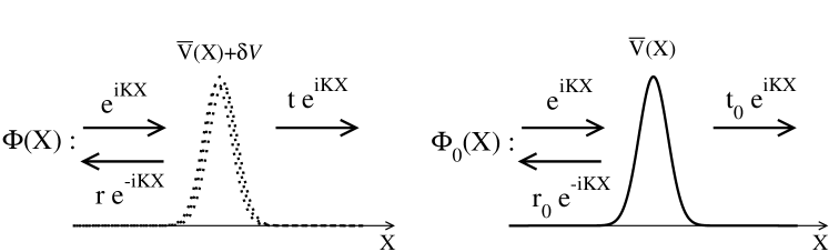
Figure 1: Left panel: In the regime of elastic scattering of a $N$-boson bright quantum soliton on a localized external potential, the centre-of-mass wavefunction $\Phi(X)$ obeys boundary conditions for $X\to\pm\infty$ with transmission and reflection amplitudes $t$ and $r$ satisfying $|t|^{2}+|r|^{2}=1$. The effective potential seen by $\Phi$ involves a non-local part $\delta\mathcal{V}$ corresponding to virtual soliton fragmentation, see Eq. (26). Right panel: In the simplest approximation, one neglects the non-local part $\delta\mathcal{V}$, only keeping the average $\bar{V}(X)$ of the single particle external potential $U(x)$ over the density profile $\rho(x|X)$ of the soliton with centre-of-mass in $X$. The resulting approximate transmission and reflection amplitudes are $t_{0}$ and $r_{0}$. Bounds on $|t-t_{0}|$ and $|r-r_{0}|$ are derived in Sec. III, and tools to evaluate the leading order corrections due to $\delta\mathcal{V}$ in the large $N$ limit are developed in Sec. IV and in Sec. V.

Theorem: If $\epsilon\eta^{1/2}<1/2$ then

$$||t|-|t_{0}||\leq|t-t_{0}| \leq \frac{|t_{0}|\epsilon\eta^{1/2}}{1-2\epsilon\eta^{1/2}}$$ (54)

$$||r|-|r_{0}||\leq|r-r_{0}| \leq \frac{|t_{0}|\epsilon}{1-2\epsilon\eta^{1/2}}.$$ (55)

The first inequalities result from the triangular inequality. The proof of the second inequalities is given in the Appendix A. In the case of an even external potential, one has simplified relations, since $\eta=1$:

Theorem: If $U(x)$ is even and $\epsilon<1/2$, then

$$||t|-|t_{0}||\leq|t-t_{0}| \leq \frac{|t_{0}|\epsilon}{1-2\epsilon}$$ (56)

$$||r|-|r_{0}||\leq|r-r_{0}| \leq \frac{|t_{0}|\epsilon}{1-2\epsilon}.$$ (57)

III.3 General results for the error potential $W(X)$

We now review some exact results derived in Castin_EPJB on the function $w(X)$ appearing in the numerator of the error potential $W(X)$, see Eqs. (47,48). The function $w(X)$ can be expressed in terms of the static structure factor of the ground state soliton for a fixed position $X$ of its centre of mass:

$$S(x,y|X) = \langle\hat{\rho}(x)\hat{\rho}(y)\rangle_{X}$$ (58)

$$= \delta(x-y)\rho(x|X)+\rho(x,y|X)$$ (59)

where $\rho(x,y|X)$ is the pair distribution function of the soliton of centre of mass localized in $X$. One has indeed

$$w(X)=\int_{\mathbf{R}^{2}}dxdy\,U(x+X)U(y+X)\\ \times[S(x,y|0)-\rho(x|0)\rho(y|0)].$$ (60)

This writing immediately reveals that $w(X)$ depends on correlations that would not be accurately treated in the classical field (Gross-Pitaevskii) approximation. From the Bethe ansatz wavefunction (6) of the soliton, Fourier transforms of $\rho(x|0)$ and $\rho(x,y|0)$ were expressed as sums of $N$ and $O(N^{2})$ terms in Castin_EPJB , which allows an exact calculation of $w(X)$.

Useful limiting cases were also studied in Castin_EPJB . For a broad external potential, with $U(x)$ varying slowly over the width of the soliton, that can be estimated by the width $\xi$ of the classical soliton given in Eq. (36), $w(X)$ is essentially proportional to the square of the second order derivative of $U$,

$$w(X)\simeq C(N)\,\xi^{4}[U^{\prime\prime}(X)]^{2}.$$ (61)

The coefficient $C(N)$ only depends on $N$, it is given as a sum of $O(N^{3})$ terms, and it has the large-$N$ asymptotic behaviour

$$C(N)\underset{N\to\infty}{\sim}N\left[\frac{2\pi^{2}}{3}+4\zeta(3)\right]$$ (62)

where $\zeta$ is the Riemann Zeta function. For a narrow external potential, centered at the origin of coordinates with a width much smaller than the soliton width $\xi$, one has for any $N$:

$$w(X)\simeq\rho(X|0)\int_{-\infty}^{+\infty}dx\,U^{2}(x).$$ (63)

Finally, irrespective of the width of $U(x)$, one can simplify Eq. (60) in the large $N$ limit by using an asymptotic expression for the pair distribution function Castin_EPJB :

$$w(X)\sim 2N\xi^{4}\int_{\mathbb{R}}dx\int_{x}^{+\infty}\!\!dy\,U^{\prime\prime}(X+x\xi)\,U^{\prime\prime}(X+y\xi)\\ \times\frac{2+y-x}{(e^{y}+1)(e^{-x}+1)}$$ (64)

where $Ng$ (and thus $\xi$) are kept fixed while $N\to+\infty$.

III.4 An improved bracketing applicable to a Dirac external potential

A limitation of the transmission and reflection coefficient bracketing of subsection III.2 is that it becomes useless when the external potential $U(x)$ is too narrow. For example, in the limiting case of a repulsive Dirac potential, $U(x)=v\delta(x)$, $v>0$, it is apparent that the quantity $\langle V^{2}\rangle_{X}$ in Eq. (47) in infinite, since it contains a sum over all the particles of $\delta^{2}(x_{i})$. As a consequence, the quantity $\epsilon$ defined in Eq. (51) is $+\infty$ and the theorem applicability condition $\epsilon<1/2$ is not satisfied.

Here, we show that a slight improvement of the derivation allows to remove this limitation. The resulting bracketing is thus more stringent, the price to pay being that the new upper bound on $|t-t_{0}|$ is more difficult to evaluate in practice.

One simply uses the fact that

$$\mathcal{Q}H\mathcal{Q}-E\mathcal{Q}\geq\mathcal{Q}H_{\rm int}\mathcal{Q}+N\inf_{x}U(x)\mathcal{Q}-E\mathcal{Q}$$ (65)

where as usual, for two Hermitian operators $A$ and $B$, $A\geq B$ means that the operator $A-B$ is non-negative, that is $\langle u|(A-B)|u\rangle\geq 0$ for any ket $|u\rangle$. Eq. (65) results from the fact that the centre-of-mass kinetic energy operator $P^{2}/2M$ is non-negative, and that each operator $U(x_{i})$ is larger than or equal to $\inf_{x}U(x)$. Since we still impose Eq. (22) on the energy $E$, and since $\mathcal{Q}H_{\rm int}\mathcal{Q}\geq[E_{0}(N)+\Delta]\mathcal{Q}$, the operator in the right-hand side of Eq. (65) is positive (within the subspace over which $\mathcal{Q}$ projects).

For two positive Hermitian operators $A$ and $B$ such that $A\geq B$, one has that

$$B^{-1}\geq A^{-1}.$$ (66)

Applying this relation for $A$ and $B$ being the left-hand side and the right-hand side operators in Eq. (65), considered within the subspace over which $\mathcal{Q}$ projects, one finds that

$$0\leq\mathcal{G}\leq\frac{\mathcal{Q}}{N\inf_{x}U(x)\mathcal{Q}+\mathcal{Q}H_{\rm int}\mathcal{Q}-E\mathcal{Q}}$$ (67)

where $\mathcal{G}$ is defined in Eq. (43). From the Cauchy-Schwarz inequality, writing $\mathcal{G}=\left(\mathcal{G}^{1/2}\right)^{2}$, we have for arbitrary kets $|u_{1,2}\rangle$ such that $\mathcal{G}^{1/2}|u_{1,2}\rangle$ are normalisable:

$$|\langle u_{1}|\mathcal{G}|u_{2}\rangle|^{2}\leq\langle u_{1}|\mathcal{G}|u_{1}\rangle\langle u_{2}|\mathcal{G}|u_{2}\rangle.$$ (68)

We apply this inequality to the kets $|u_{1}\rangle$ and $|u_{2}\rangle$ defined in Eqs.(40,41), that do not need to be normalisable, and we use the upper bound on the operator $\mathcal{G}$ to obtain for arbitrary centre-of-mass wavefunctions $\Phi_{1,2}(X)$ (not diverging too fast at infinity):

$$|\langle\Phi_{1}|\delta\mathcal{V}|\Phi_{2}\rangle|\leq\left[\langle\Phi_{1}|W_{\rm imp}(\hat{X})|\Phi_{1}\rangle\langle\Phi_{2}|W_{\rm imp}(\hat{X})|\Phi_{2}\rangle\right]^{1/2},$$ (69)

where the improved error potential is positive:

$$W_{\rm imp}(X)=\langle\phi|V\mathcal{Q}\frac{\mathcal{Q}}{N\inf_{x}U(x)\mathcal{Q}+\mathcal{Q}H_{\rm int}\mathcal{Q}-E\mathcal{Q}}\mathcal{Q}V|\phi\rangle.$$ (70)

Thanks to the occurrence of the internal kinetic energy operator of the particles within $H_{\rm int}$ in the denominator, this error potential remains finite even when the barrier is a repulsive $\delta$ potential.

The reasoning of subsection III.1 may then be reproduced, replacing the error potential $W$ by the improved one. Similarly to Eqs.(51,52) we thus define

$$\epsilon_{\rm imp} = \frac{M\langle\Phi_{0}|W_{\rm imp}(\hat{X})|\Phi_{0}\rangle}{\hbar^{2}K|t_{0}|}$$ (71)

$$\eta_{\rm imp} = \frac{\langle\tilde{\Phi}_{0}|W_{\rm imp}(\hat{X})|\tilde{\Phi}_{0}\rangle}{\langle\Phi_{0}|W_{\rm imp}(\hat{X})|\Phi_{0}\rangle}$$ (72)

where, as in subsection III.1, $\Phi_{0}(X)$ and $\tilde{\Phi}_{0}(X)$ are the centre-of-mass scattering wavefunctions with incoming wavevector $K$ and $-K$ respectively, for the potential $\bar{V}(X)$. One then has:
Improved theorem: If $\epsilon_{\rm imp}\eta_{\rm imp}^{1/2}<1/2$ then

$$||t|-|t_{0}||\leq|t-t_{0}| \leq \frac{|t_{0}|\epsilon_{\rm imp}\eta_{\rm imp}^{1/2}}{1-2\epsilon_{\rm imp}\eta_{\rm imp}^{1/2}}$$ (73)

$$||r|-|r_{0}||\leq|r-r_{0}| \leq \frac{|t_{0}|\epsilon_{\rm imp}}{1-2\epsilon_{\rm imp}\eta_{\rm imp}^{1/2}},$$ (74)

where $r,t$ are the exact reflection and transmission coefficients, and $r_{0},t_{0}$ are the reflection and transmission coefficients for $\Phi_{0}$, that is for the potential $\bar{V}(X)$. As in subsection III.1, a simpler form is obtained for an even external potential $U(x)=U(-x)$, in which case $\eta_{\rm imp}=1$.

III.5 General results for the improved error potential $W_{\rm imp}(X)$

A general calculation of $W_{\rm imp}(X)$ with the Bethe ansatz, amounting to evaluating an internal dynamic structure factor of the ground state soliton with fixed centre-of-mass position, may be doable with the techniques developed in Caux1 ; Caux2 but this is beyond the scope of this paper. On the contrary, a large $N$ limit (for fixed $Ng$ and $\xi$) is straightforward to obtain from the Bogoliubov technique exposed in Sec. IV: In Eq. (90) one simply has to omit the centre-of-mass kinetic energy term and to replace $\bar{V}(X)$ by the lower bound $N\inf_{x}U(x)$:

$$W_{\rm imp}(X)\underset{N\to+\infty}{\sim}\int_{\mathbb{R}}\frac{dk}{2\pi}\frac{|\Gamma_{k}(X)|^{2}}{N\inf_{x}U(x)+\frac{\hbar^{2}k^{2}}{2m}+\Delta-\frac{\hbar^{2}K^{2}}{2M}}$$ (75)

where the amplitude $\Gamma_{k}(X)$ is given by (88) and $\Delta\simeq\hbar^{2}/(8m\xi^{2})$, see (9).

When the external potential is a repulsive delta potential, $U(x)=v\delta(x)$, $v>0$, with $\inf_{x}U(x)=0$, the integral over $k$ can be calculated:

$$W_{\rm imp}(X)\sim\frac{2Nmv^{2}\xi}{\gamma\hbar^{2}}\phi_{0}^{2}(X)\left[1-\frac{32(\gamma+2)}{(\gamma+1)^{2}}\xi^{3}\phi_{0}^{\prime 2}(X)\right]$$ (76)

where $\gamma\in(0,1)$ is such that

$$\gamma^{2}=1-\frac{\hbar^{2}K^{2}}{2M\Delta}.$$ (77)

As expected, (76) diverges when the incoming centre-of-mass kinetic energy tends to the gap $\Delta$, but it diverges as $1/\gamma$, whereas the error potential $W(X)$ generically diverges as $1/\gamma^{2}$ for a non-negative $U(x)$, see Eq. (48).

This indicates that the improved bound can have some interest also for a broad barrier. In the large $N$ limit, when $U(X)$ has a width $b\gg\xi$, we find using (89) and assuming for simplicity that $\inf_{x}U(x)=0$:

$$W_{\rm imp}(X)\underset{b\gg\xi}{\simeq}\frac{8\pi^{2}N\xi^{4}}{\Delta}[U^{\prime\prime}(X)]^{2}\\ \times\int_{\mathbb{R}}\frac{dk}{2\pi}[(1+k^{2})^{2}(\gamma^{2}+k^{2})\cosh^{2}(\pi k/2)]^{-1},$$ (78)

where the integral may be expressed analytically if necessary, in particular in terms of the derivative of the digamma function, using the residue theorem.

IV Large $N$ limit of the effective potential for a $O(1/N)$ barrier

We calculate a large $N$ expansion of the non-local part $\delta\mathcal{V}$ of the effective potential in Eq. (26), using Bogoliubov theory, in the case where the external potential $U$ experienced by each particle scales as $1/N$ and the soliton width $\xi$ is fixed (because $Ng$ is fixed). This physically convenient scaling with $N$ ensures that the potential $\bar{V}$ has a well-defined non-zero limit for $N\to+\infty$.

IV.1 Bogoliubov theory in brief

We use Bogoliubov theory to dress with quantum fluctuations the classical soliton of single particle wavefunction (38). Since $\phi_{0}$ is centered at the origin of coordinates, we shall shift the positions of the particles as $x_{i}\to x_{i}+X$ where $X$ is the fixed position of the centre of mass of the quantum soliton. In the number conserving theory Gardiner ; CastinDum , one splits the bosonic field operator as

$$\hat{\psi}(x)=\hat{a}_{0}\phi_{0}(x)+\hat{\psi}_{\perp}(x)$$ (79)

where $\hat{a}_{0}$ annihilates a particle in the mode $\phi_{0}$ and the field $\hat{\psi}_{\perp}(x)$ is orthogonal to the field $\phi_{0}(x)$. We introduce the modulus-phase representation Girardeau ; Nieto , which is an excellent approximation for large $N$ (when the probability of having an empty mode $\phi_{0}$ is negligible):

$$\hat{a}_{0}=e^{i\hat{\theta}}\hat{n}_{0}^{1/2},$$ (80)

where the Hermitian phase operator $\hat{\theta}$ is conjugate to the number operator $\hat{n}_{0}=\hat{a}_{0}^{\dagger}\hat{a}_{0}$, $[\hat{n}_{0},\hat{\theta}]=i$. The phase $\hat{\theta}$ is formally eliminated by its inclusion with the field $\hat{\psi}_{\perp}$ in the number conserving field

$$\hat{\Lambda}(x)=e^{-i\hat{\theta}}\hat{\psi}_{\perp}(x).$$ (81)

Conservation of the total number of particles allows to eliminate $\hat{n}_{0}$ in terms of $\hat{\Lambda}$ and of the total number operator $\hat{N}$. In the large $N$ limit (with $Ng$ fixed), it is found that $\hat{\Lambda}=O(1/\xi^{1/2})$ whereas $\hat{a}_{0}$ scales as $N^{1/2}$, which allows a systematic expansion of the Hamiltonian in powers of $\hat{\Lambda}$. Keeping terms up to order $O(\hat{\Lambda}^{2})$ in $H_{0}$ leads to the Bogoliubov approximation for $N$ particles,

$$H_{0}\simeq E_{0}^{\rm Bog}(N)+\frac{\hat{P}^{2}}{2Nm}+\int_{\mathbf{R}}\frac{dk}{2\pi}\epsilon_{k}\hat{b}_{k}^{\dagger}\hat{b}_{k}$$ (82)

with the gapped Bogoliubov spectrum in terms of the quasiparticle wavevector $k$ and the Gross-Pitaevskii chemical potential $\mu_{0}$:

$$\epsilon_{k}=|\mu_{0}|+\frac{\hbar^{2}k^{2}}{2m}\ \ \ \mbox{\rm where}\ \ \ \mu_{0}=-\frac{\hbar^{2}}{8m\xi^{2}}.$$ (83)

The quasi-particle annihilation and creation operators $\hat{b}_{k}$ and $\hat{b}_{k}^{\dagger}$ obey the usual bosonic commutation relations on the open line, $[\hat{b}_{k},\hat{b}_{k^{\prime}}^{\dagger}]=2\pi\delta(k-k^{\prime})$. Due to the translational symmetry breaking, a Goldstone mode appears, with a massive term $\propto\hat{P}^{2}$ in the Hamiltonian, the field variable $\hat{P}$ (scaling as $N^{1/2}$) representing at the Bogoliubov level the total momentum of the system, and being conjugate to the field variable $\hat{Q}$ (scaling as $1/N^{1/2}$) giving at the Bogoliubov level the fluctuations of the centre-of-mass position of the system: This reproduces the structure of Eq. (4). The modal field expansion is then

$$\hat{\Lambda}(x) = -N^{1/2}\phi_{0}^{\prime}(x)\hat{Q}+\frac{i}{\hbar N^{1/2}}x\phi_{0}(x)\hat{P}$$ (84)

$$+ \int_{\mathbf{R}}\frac{dk}{2\pi}[u_{k}(x)\hat{b}_{k}+v_{k}^{*}(x)\hat{b}_{k}^{\dagger}].$$

The Bogoliubov mode functions are known exactly Kaup and are given with the present notations in Castin_EPJB . They are orthogonal to $\phi_{0}$, and one has also that $u_{k}+v_{k}$ is orthogonal to $x\phi_{0}(x)$. This is apparent on the useful form:

$$\phi_{0}(x)[u_{k}(x)+v_{k}(x)]=\frac{4\xi^{2}}{(1+2i|k|\xi)^{2}}\frac{d^{2}}{dx^{2}}\left[e^{ikx}\phi_{0}(x)\right].$$ (85)

IV.2 Bogoliubov expression of $\delta\mathcal{V}$

To calculate $\delta\mathcal{V}$ given by Eq. (31), we first have to express the operator $V$ in the Bogoliubov framework. To the same level of approximation as for the Hamiltonian $H_{0}$, that is neglecting terms that are cubic or more in $\hat{\Lambda}$, we obtain

$$\sum_{i=1}^{N}U(X+x_{i})\simeq(N-\int_{\mathbb{R}}dx\,\hat{\Lambda}^{\dagger}\hat{\Lambda})\int_{\mathbb{R}}dx\,\phi_{0}^{2}(x)U(X+x)\\ +N^{1/2}\int_{\mathbb{R}}dx\,[\hat{\Lambda}(x)+\hat{\Lambda}^{\dagger}(x)]\phi_{0}(x)U(X+x)\\ +\int_{\mathbb{R}}dx\,U(X+x)\hat{\Lambda}^{\dagger}(x)\hat{\Lambda}(x).$$ (86)

It is clear that, in the Bogoliubov framework, applying the projector $\mathcal{P}$ of the full quantum theory amounts to projecting onto the vacuum $|0\rangle_{\rm Bog}$ of all the quasiparticle annihilation operators $\hat{b}_{k}$, so that applying $\mathcal{Q}$ amounts to projecting onto the subspace with at least one quasiparticle excitation. In the Bogoliubov evaluation of $\mathcal{Q}V|\phi\rangle$, the leading term explicitly scaling as $N$ in Eq. (86) gives a vanishing contribution, so we keep the subleading $N^{1/2}$ term of (86). Similarly, due to the projector $\mathcal{Q}$, we keep only the contributions involving $\hat{b}_{k}^{\dagger}$ in Eq. (84) to obtain

$$\mathcal{Q}V|\phi\rangle\simeq\int_{\mathbb{R}}\frac{dk}{2\pi}\,\Gamma_{k}(X)\hat{b}_{k}^{\dagger}|0\rangle_{\rm Bog}$$ (87)

with the amplitudes depending parametrically on $X$:

$$\Gamma_{k}(X)=N^{1/2}\int_{\mathbb{R}}dx\,[u_{k}^{*}(x)+v_{k}^{*}(x)]\phi_{0}(x)U(X+x)\\ =\frac{4\xi^{2}N^{1/2}}{(1-2i|k|\xi)^{2}}\int_{\mathbb{R}}dx\,e^{-ikx}\phi_{0}(x)U^{\prime\prime}(X+x)$$ (88)

where we used (85). The integral over $x$ is typically cut to $|x|\lesssim\xi$ by the rapidly decreasing function $\phi_{0}(x)$. For an external potential narrower than $\xi$, $|\Gamma_{k}(X)|$ varies with $X$ at the length scale $\xi$. For a broad external potential, varying at a scale $b\gg\xi$, we expect that $\Gamma_{k}(X)$ varies with $X$ at the length scale $b$. This can be made quantitative by expanding $U^{\prime\prime}(X+x)$ in the integrand of Eq. (88) to zeroth order in $x$:

$$\Gamma_{k}(X)\underset{b\gg\xi}{\simeq}\frac{4\pi\xi^{5/2}N^{1/2}U^{\prime\prime}(X)}{(1-2i|k|\xi)^{2}\cosh(\pi k\xi)}.$$ (89)

It remains to estimate the denominator $E\mathcal{Q}-\mathcal{Q}H\mathcal{Q}$ with Bogoliubov theory. Within the subspace with one Bogoliubov excitation, the leading term explicitly scaling as $N$ in Eq. (86) gives a non-zero contribution which is actually $O(1)$ since $U=O(1/N)$. This contribution does not affect the quasiparticle, it is a scalar depending on $X$ only, and it simply corresponds to the mean-field (Gross-Pitaevskii) approximation for $\bar{V}(X)$. The subleading term in Eq. (86), which changes the number of quasiparticles by $\pm 1$, is more involved since it couples the single-quasiparticle subspace to the two-quasiparticle subspace. However, its contribution is $O(N^{1/2}U)=O(1/N^{1/2})$ and may be neglected at the present order.

We finally obtain in the large $N$ limit, for $U=O(1/N)$ and fixed $Ng$, the leading term of $\delta\mathcal{V}$, scaling as $1/N$:

$$\delta\mathcal{V}\sim\int_{\mathbb{R}}\frac{dk}{2\pi}\Gamma_{k}^{*}(X)\\ \times\left\{E-\left[\frac{P^{2}}{2M}+E_{0}(N)+\epsilon_{k}+\bar{V}(X)\right]\right\}^{-1}\Gamma_{k}(X).$$ (90)

Here $P=-i\hbar\partial_{X}$ is the centre-of-mass momentum operator of the full quantum theory. The expansion of $\bar{V}$ up to the same order (neglecting $o(1/N)$) is directly given by (39). One may then solve numerically the resulting approximate form of Eq. (26), which is made delicate by the non-local nature of (90). More simply, one may treat (90) as a first order perturbation in the $\bar{V}$ scattering problem using the formulation of the Appendix A [see below Eq. (150)], to obtain:

$$t-t_{0} \simeq -\frac{iM}{\hbar^{2}K}\langle\tilde{\Phi}_{0}^{*}|\delta\mathcal{V}|\Phi_{0}\rangle$$ (91)

$$r-r_{0} \simeq -\frac{iM}{\hbar^{2}K}\langle\Phi_{0}^{*}|\delta\mathcal{V}|\Phi_{0}\rangle,$$ (92)

the ket $|\Phi_{0}^{*}\rangle$ corresponding to the wavefunction $\Phi_{0}^{*}(X)$.

V Born-Oppenheimer-like approach

In molecular physics, one often uses the so-called Born-Oppenheimer approximation: One diagonalises the electronic problem for fixed positions of the nuclei, obtaining a ground state electronic energy that then serves as a potential for the nuclei BO ; IFT . It is natural to try to apply a similar approach to our soliton scattering problem. The “heavy” particle then corresponds to the centre of mass of the soliton, and the “light” particles are the internal degrees of freedom of the soliton. We thus split the $N$-body Hamiltonian as $H=H^{\rm heavy}+H^{\rm light}$, with

$$H^{\rm heavy} = \frac{P^{2}}{2M}+NU(X)$$ (93)

$$H^{\rm light} = H_{\rm int}+\sum_{i=1}^{N}[U(x_{i})-U(X)].$$ (94)

In $H^{\rm heavy}$, we have included the external potential that the soliton would feel if all the particles were localized in the centre-of-mass position $X$. We expect this term $NU(X)$ to constitute already a good approximation when the external potential is much broader than the soliton width $\xi$. To go beyond this zeroth order approximation, the idea is to calculate the ground state energy $E_{0}^{\rm light}(X)$ of $H^{\rm light}$ for a fixed value of the centre-of-mass position. This energy then provides a correction to the potential $NU(X)$ experienced by the centre of mass of the soliton. An important condition for the Born-Oppenheimer approximation to hold is that $E_{0}^{\rm light}(X)$ is well separated from the excited state energies of $H^{\rm light}$ for a fixed $X$, so that the presence of the solitonic internal gap again plays an important role here.

More precisely, we call $|\chi(X)\rangle$ the ground state of the internal Hamiltonian $H^{\rm light}$ corresponding to the eigenvalue $E_{0}^{\rm light}(X)$, and we put forward the Born-Oppenheimer-like ansatz for the $N$-body state vector:

$$\langle X|\psi\rangle_{\rm BO}=\Phi(X)|\chi(X)\rangle$$ (95)

where the ket $|X\rangle$ represents the centre of mass perfectly localized in $X$ and the internal ket $|\chi(X)\rangle$, normalized to unity, parametrically depends on $X$ . We then insert the ansatz into Schrödinger’s equation $E|\psi\rangle=H|\psi\rangle$ and project with $\langle\chi(X)|$ to obtain

$$E\Phi(X)=-\frac{\hbar^{2}}{2M}\frac{d^{2}}{dX^{2}}\Phi(X)+\Big{[}NU(X)+E_{0}^{\rm light}(X)\\ -\frac{\hbar^{2}}{2M}\langle\chi(X)|\frac{d^{2}}{dX^{2}}|\chi(X)\rangle\Big{]}\Phi(X).$$ (96)

Note that we keep here the so-called Born-Oppenheimer diagonal correction coming from the $X$ dependence of the internal state in the ansatz.

In practice, to evaluate $E_{0}^{\rm light}(X)$ and the corresponding eigenvector, we use perturbation theory, treating $\sum_{i=1}^{N}[U(x_{i})-U(X)]$ as a perturbation of $H_{\rm int}$. For example, to second order in this perturbation, we obtain:

$$E_{0}^{\rm light}(X)\simeq E_{0}(N)-NU(X)+\langle\phi|V|\phi\rangle\\ +\langle\phi|V\mathcal{Q}\frac{\mathcal{Q}}{E_{0}(N)\mathcal{Q}-\mathcal{Q}H_{\rm int}\mathcal{Q}}\mathcal{Q}V|\phi\rangle,$$ (97)

where, as in the previous sections, the internal ket $|\phi\rangle$ is the free space ground state soliton of energy $E_{0}(N)$, $\mathcal{P}$ projects orthogonally onto $|\phi\rangle$ and the supplementary projector $\mathcal{Q}=1-\mathcal{P}$ projects onto the internal excited states of the system. Remarkably, the third term in the right-hand side of Eq. (97) exactly coincides with $\bar{V}(X)$. To first order in the perturbation theory, the internal ground state in presence of the external potential is

$$|\chi(X)\rangle\simeq\mathcal{F}(X)\left[|\phi\rangle+\frac{\mathcal{Q}}{E_{0}(N)\mathcal{Q}-\mathcal{Q}H_{\rm int}\mathcal{Q}}\mathcal{Q}V|\phi\rangle\right].$$ (98)

The normalization factor $\mathcal{F}$ should for consistency only weakly deviate from unity, which imposes a limit on the strength of the external potential.

We apply the above approximation scheme in the large $N$ limit, where it makes the most sense, fixing $Ng$ (and thus the soliton width $\xi$). We can then use the Bogoliubov approach, and following the lines of section IV:

$$E_{0}^{\rm light}(X)\simeq E_{0}^{\rm Bog}(N)-NU(X)+\bar{V}(X)\\ +\int_{\mathbb{R}}\frac{dk}{2\pi}\frac{|\Gamma_{k}(X)|^{2}}{-\epsilon_{k}},$$ (99)

where $\Gamma_{k}(X)$ is given by Eq. (88). Also, the Born-Oppenheimer diagonal correction is approximated with Bogoliubov theory as

$$-\frac{\hbar^{2}}{2M}\langle\chi(X)|\frac{d^{2}}{dX^{2}}|\chi(X)\rangle\simeq\frac{\hbar^{2}}{2M}\int_{\mathbb{R}}\frac{dk}{2\pi}\frac{|\frac{d}{dX}\Gamma_{k}(X)|^{2}}{\epsilon_{k}^{2}}.$$ (100)

It is about $N$ times smaller than the Bogoliubov term appearing in $E_{0}^{\rm light}(X)$, see the last term in Eq. (99), and we neglect it in the large $N$ limit. To summarize, in the Born-Oppenheimer approximation for large $N$, we find for the soliton wavefunction an equation of the form (26) with the non-local $\delta\mathcal{V}$ approximated by the local form [after use of Eq. (88)]

$$\delta\mathcal{V}_{\rm BO}\simeq\int_{\mathbb{R}}\frac{dk}{2\pi}\frac{|\Gamma_{k}(X)|^{2}}{-\epsilon_{k}}=-\frac{N\xi}{8\Delta}\int_{\mathbb{R}^{2}}dxdy\,\phi_{0}(x)\phi_{0}(y)U^{\prime\prime}(X+x)U^{\prime\prime}(X+y)e^{-|x-y|/2\xi}[(x-y)^{2}+6\xi|x-y|+12\xi^{2}]$$ (101)

The integral can be evaluated for a delta external potential, $U(x)=v\delta(x)$, leading to :

$$\delta\mathcal{V}_{\rm BO}\simeq-\frac{5}{4}N\frac{mv^{2}}{\hbar^{2}}\left\{\xi\phi_{0}^{2}(X)+\frac{48}{5}\xi^{5}\left[\phi_{0}^{\prime\prime}(X)\right]^{2}\right\}.$$ (102)

It is interesting to compare Eq. (101) to the result Eq. (90) that was obtained in a different way. At first sight, Eq. (90) and Eq. (101) look widely different, because of the more complicated energy denominator in Eq. (90) that involves both $P^{2}/2M$ and $\bar{V}(X)$, rather then a simple c-number quantity such as $\epsilon_{k}$. We have identified a limiting case where the two expressions are close, when the typical wavevector $K$ of $\Phi(X)$ is much larger than $1/\xi$, and $\delta\mathcal{V}$ has a small perturbative effect on the scattering state $\Phi$. Since the relevant $k$ are $O(1/\xi)$ in the integral over $k$, $\Gamma_{k}(X)$ varies at a length scale of order $\xi$ or larger, see discussion below Eq. (88), whereas $\Phi(X)$ varies over a much smaller length scale $1/K$. The spatial derivatives of $\Gamma_{k}(X)\Phi(X)$ are thus well approximated by taking the derivatives of $\Phi(X)$ only, e.g.

$$P\Gamma_{k}(X)|\Phi\rangle\underset{K\xi\gg 1}{\simeq}\Gamma_{k}(X)P|\Phi\rangle,$$ (103)

where $P=-i\hbar\partial_{X}$ is the centre-of-mass momentum operator. We can then approximately commute the energy denominator with $\Gamma_{k}(X)$ in Eq. (90). The last step is to realise that, if $\delta\mathcal{V}$ is small enough, $\Phi(X)$ will be close to the scattering state of energy $E$ for the potential $E_{0}(N)+\bar{V}(X)$ so that

$$\left\{E-\left[\frac{P^{2}}{2M}+E_{0}(N)+\epsilon_{k}+\bar{V}(X)\right]\right\}^{-1}|\Phi\rangle\simeq-\frac{1}{\epsilon_{k}}|\Phi\rangle$$ (104)

and we recover the Born-Oppenheimer result Eq. (101).

VI Applications of the formalism

VI.1 Centre-of-mass wavepacket splitting

We apply our formalism to the proposal of PRL2009 for the production of Schrödinger’s cat-like states by elastic scattering of a soliton on a barrier: One sends the ground state soliton with a quasi-monochromatic centre-of-mass wavepacket, that is centered in $K$-space around $\bar{K}$ with a width $\Delta K\ll\bar{K}$, on a barrier of adjusted height such that the transmission and reflection amplitudes have the same modulus $1/\sqrt{2}$. This prepares the gas in a coherent superposition of all the particles being to the right and to the left of the barrier with equal probability amplitudes. For the experimental decoherence rate estimated in PRL2009 , this in principle allows to prepare a gas of $N\simeq 100$ lithium 7 atoms in a coherent superposition of being at two different locations separated by $\simeq 100\,\mu$m. We thus restrict to the most interesting large-$N$ limit. As the potential barrier may be produced with a focused Gaussian laser beam, we can assume that $U(x)$ is a repulsive Gaussian of width $b$ (the so-called waist of the laser beam):

$$U(x)=U_{0}e^{-2x^{2}/b^{2}},\ \ \ U_{0}>0,$$ (105)

so that the potential $\bar{V}(X)$ is also even and bell shaped. We shall also assume, as in PRL2009 , that

$$\frac{\hbar^{2}\bar{K}^{2}}{2M}=\frac{\Delta}{2},$$ (106)

so that in the large $N$ limit,

$$\bar{K}\sim\frac{N^{1/2}}{2\sqrt{2}\xi}.$$ (107)

Having a significantly smaller $\bar{K}$ would indeed uselessly slow down the Schrödinger’s cat formation process. Having a significantly larger $\bar{K}$ is forbidden by the elasticity condition (22).

Case $b\gg\xi$: This broad barrier case is experimentally the typical one, since the waist of a focused laser beam is a few microns, whereas $\xi\lesssim 1\mu$m PRL2009 . Then $\bar{V}(X)\simeq NU(X)$, and the width of $\bar{V}$ is also of order $b$. Since $\bar{K}b\propto N^{1/2}b/\xi$ is much larger than unity, the scattering problem of the centre-of-mass on $\bar{V}(X)$ is in the semiclassical regime, where the transmission and reflection amplitudes at incoming wavevector $K$ have the approximate expressions, see Eqs. (3.49,3.58,4.23) in Berry :

$$t_{0} \simeq \frac{e^{-\lambda(K)}e^{i[\alpha(K)-\beta(K)]}}{[1+e^{-2\lambda(K)}]^{1/2}}$$ (108)

$$r_{0} \simeq \frac{-i\,e^{i[\alpha(K)-\beta(K)]}}{[1+e^{-2\lambda(K)}]^{1/2}}$$ (109)

$$\lambda(K) = \int_{X_{-}}^{X_{+}}dX\ (-i)K(X)\geq 0$$ (110)

$$\alpha(K) = 2KX_{-}+2\int_{-\infty}^{X_{-}}dX[K(X)-K]$$ (111)

$$\beta(K) = \frac{\lambda(K)}{\pi}\ln\left|\frac{\lambda(K)}{\pi e}\right|\!+\!\arg\Gamma\!\left(\!\frac{1}{2}-\frac{i\lambda(K)}{\pi}\!\right)$$ (112)

$$K(X) = \left[K^{2}-\frac{2M\bar{V}(X)}{\hbar^{2}}\right]^{1/2}$$ (113)

Here $X_{-}\leq 0$ and $X_{+}=-X_{-}$ are the two classical turning points for an incoming energy below the maximum $V_{0}$ of $\bar{V}$, and $K(X)$ is either in $\mathbb{R}^{+}$ or in $i\mathbb{R}^{+}$ if $X$ is in the classically allowed or forbidden region. For an incoming energy larger than $V_{0}$, one has to use analytic continuation Berry . The phase $\beta(K)$ is given in Berry , and the extra phase $\alpha(K)$ is due to our different choice for the phase reference point. We also recall the WKB approximation for $\Phi_{0}(X)$ in the classically allowed region:

$$\!\!\!\!\!\!\Phi_{0}(X)\!\!\!\! \stackrel{{\scriptstyle X<X_{-}}}{{\simeq}} \!\!\!\![K/K(X)]^{1/2}\Big{[}e^{iKX}e^{i\int_{-\infty}^{X}dx[K(x)-K]}$$ (114)

$$+r_{0}e^{-iKX}e^{-i\int_{-\infty}^{X}dx[K(x)-K]}\Big{]}$$

$$\!\!\!\!\!\!\Phi_{0}(X)\!\!\!\! \stackrel{{\scriptstyle X>X_{+}}}{{\simeq}} \!\!\!\![K/K(X)]^{1/2}t_{0}e^{iKX}e^{i\int_{+\infty}^{X}dx[K(x)-K]}$$ (115)

We then see that a transmission probability of $1/2$ is achieved in the semiclassical formula (108) for an energy equal to $V_{0}$, that is for a momentum

$$K_{1/2}=\frac{(2MV_{0})^{1/2}}{\hbar}.$$ (116)

Away from this value of $K$, $|t_{0}|^{2}$ will drop rapidly to zero or rise rapidly to one. A local formula is obtained by approximating the top of $\bar{V}(X)$ around $X=0$ by a parabola, so that

$$|t_{0}|^{2}\simeq\frac{1}{1+\exp[(K_{1/2}-K)/\delta K]}$$ (117)

with

$$\delta K=\frac{1}{2\pi}\left(\frac{|\bar{V}^{\prime\prime}(0)|}{2\bar{V}(0)}\right)^{1/2}.$$ (118)

For large $N$, one finds $\delta K\simeq 1/(\sqrt{2}\pi b)$ so that one is experimentally in the regime $\Delta K\gg\delta K$. In what follows, we thus adjust the barrier height to have $K_{1/2}=\bar{K}$. Then, with Eq. (106),

$$NU_{0}\simeq V_{0}=\frac{\Delta}{2}.$$ (119)

Finally, we evaluate the parameter $\epsilon$ of (51) appearing in the bracketing (56,57) (that can be used here since $U(x)$ and $\bar{V}(X)$ are even), for the physically most relevant case $K=\bar{K}=K_{1/2}$. We use the large-$N$ estimate for a broad barrier, see Eqs. (61,62), and the simplest estimate (neglecting rapidly oscillating terms):

$$|\Phi_{0}(X)|^{2}\propto\frac{K_{1/2}}{K(X)}$$ (120)

with $K(X)$ defined in (113) and a proportionality factor equal to $1+|r_{0}|^{2}=3/2$ for $X<0$ and to $|t_{0}|^{2}=1/2$ for $X>0$. Since $K(X)$ vanishes linearly in the classical turning point $X=0$, we get a logarithmic divergence in the resulting approximation for $\langle\Phi_{0}|W|\Phi_{0}\rangle$, that we cut by introducing the quantum length scale $a_{\rm ho}\ll b$ associated to the Schrödinger’s equation in the inverted parabola approximating $\bar{V}(X)$ close to its maximum :

$$a_{\rm ho}=\frac{\hbar^{1/2}}{(M|\bar{V}^{\prime\prime}(0)|)^{1/4}}\simeq\left(\frac{b}{\sqrt{2}\bar{K}}\right)^{1/2}\simeq\left(\frac{2b\xi}{N^{1/2}}\right)^{1/2}$$ (121)

Keeping only the logarithmically diverging contribution amounts to approximating the matrix element as

$$\langle\Phi_{0}|W(\hat{X})|\Phi_{0}\rangle\simeq 2W(0)\int_{a_{\rm ho}}^{b}dX\,\frac{b}{X\sqrt{2}},$$ (122)

which leads to the estimate

$$\epsilon\simeq\left(\frac{2\xi}{b}\right)^{3}\left(\frac{2}{N}\right)^{1/2}\left[\frac{\pi^{2}}{3}+2\zeta(3)\right]\ln(b/a_{\rm ho}).$$ (123)

In conclusion, for $|t_{0}|^{2}\simeq 1/2$ in the broad barrier case, we find in the large $N$ limit (where $\epsilon\ll 1$):

$$|t-t_{0}|=O\left[\frac{(\xi/b)^{3}}{N^{1/2}}\ln\left(N^{1/2}b/\xi\right)\right],$$ (124)

as already given in PRL2009 .

Case $b\ll\xi$: For a narrow barrier,

$$\bar{V}(X)\simeq\rho(X|0)\int_{-\infty}^{+\infty}dx\ U(x).$$ (125)

In the large $N$ limit, replacing $\rho(X|0)$ by its classical field approximation, that is the leading term in the right-hand side of (39), gives

$$\bar{V}(X)\simeq\frac{V_{0}}{\cosh^{2}(X/b_{\rm eff})}$$ (126)

with

$$V_{0} = \frac{N}{4\xi}\int_{-\infty}^{+\infty}dx\ U(x)$$ (127)

$$b_{\rm eff} = 2\xi.$$ (128)

Although the resulting scattering problem for $\Phi_{0}(X)$ then becomes exactly solvable Landau , we simply reuse the semiclassical reasoning of the previous (broad-barrier) case, since $\bar{K}b_{\rm eff}\simeq(N/2)^{1/2}\gg 1$ is again in the semiclassical regime. At half transmission probability,

$$\frac{NU_{0}}{\Delta}\simeq\left(\frac{8}{\pi}\right)^{1/2}\frac{\xi}{b}\gg 1$$ (129)

so that $NU_{0}$ is now much larger than the gap $\Delta$, contrarily to the broad barrier case. The harmonic oscillator length used in the cutting procedure is found to be $a_{\rm ho}\simeq b_{\rm eff}(2/N)^{1/4}$. We use the equivalent of Eq. (122) and we estimate $W(0)$ from Eq. (63). At half transmission probability, we finally obtain from the simple bracketing (56,57):

$$|t-t_{0}|\lesssim\frac{\xi/b}{N^{1/2}}\frac{\ln(N/2)}{(2\pi)^{1/2}}.$$ (130)

As expected, this bound diverges for $b\to 0$ (at fixed $N$), since $U(x)$ then approaches a Dirac potential, for which the use of the improved bracketing (73,74) is more appropriate and leads at half transmission for large $N$ to

$$|t-t_{0}|\lesssim\frac{\ln(N/2)}{8N^{1/2}},$$ (131)

where Eq. (76) was used with $v=U_{0}b\,(\pi/2)^{1/2}$.

The Born-Oppenheimer prediction: For the delta external potential $U(x)=v\delta(x)$, it is interesting to compare the upper bound (131) to the result of Sec. V. In the present large $N$ limit, one can treat $\mathcal{V}_{\rm BO}$ with first order perturbation theory similarly to Eqs. (91,92) and one can use the expression (102) for $\mathcal{V}_{\rm BO}$. In the resulting perturbative expression for $t-t_{0}$, one can approximate the various quantities by their $N\to+\infty$ limit, in particular the scattering wavefunction $\Phi_{0}(X)$ at incoming wavevector $K$ may be replaced by the scattering wavefunction $\Phi_{0}^{(0)}(X)$ of the $1/\cosh^{2}$ potential of Eq. (126), which is exactly expressed in terms of an hypergeometric function Landau , with the transmission amplitude

$$t_{0}^{(0)}=\frac{\Gamma(\frac{1}{2}+is-iKb_{\rm eff})\Gamma(\frac{1}{2}-is-iKb_{\rm eff})}{\Gamma(1-iKb_{\rm eff})\Gamma(-iKb_{\rm eff})}$$ (132)

with

$$s=\left(\frac{2Mb_{\rm eff}^{2}}{\hbar^{2}}V_{0}-\frac{1}{4}\right)^{1/2}.$$ (133)

Here, to zeroth order in $1/N$, we have $Kb_{\rm eff}\simeq(N/2)^{1/2}$ as in Eq. (107), and $s\simeq Kb_{\rm eff}$ due to the half-transmission condition $|t_{0}^{(0)}|\simeq|t_{0}|=1/\sqrt{2}$, so that $Nmv^{2}/\hbar^{2}\simeq\hbar^{2}/(16M\xi^{2})$. Further expressing Eq. (102) in terms of the variable $\theta=\tanh(X/b_{\rm eff})$, we obtain

$$t-t_{0}\simeq\frac{i}{8(N/2)^{1/2}}\int_{-1}^{1}d\theta(1-\frac{3}{2}\theta^{2}+\frac{3}{2}\theta^{4})\Phi_{0}^{(0)}(X)\Phi_{0}^{(0)}(-X).$$ (134)

The terms proportional to $\theta^{2}$ and $\theta^{4}$ vanish in $\theta=0$, which allows to directly use the WKB forms (114,115): at half-transmission, $K(X)=K|\theta|$ so that

$$\Phi_{0}^{(0)}(X)\Phi_{0}^{(0)}(-X)\simeq\frac{t_{0}^{(0)}}{\theta}\left(1-\frac{i}{\sqrt{2}}e^{-iKb_{\rm eff}\ln(1-\theta^{2})}\right),$$ (135)

and one finds as expected that the rapidly oscillation bit gives a negligible contribution to the integral. Note that the semiclassical approximation gives

$$t_{0}^{(0)}\simeq\frac{e^{-2iKb_{\rm eff}\ln 2}}{\sqrt{2}}$$ (136)

in agreement with the Stirling asymptotic equivalent of (132) for $s=Kb_{\rm eff}\to+\infty$.

On the contrary, the constant term in between the parenthesis in Eq. (134) cannot be treated with the simple WKB approximation (135): As already discussed above, this simple approximation is inaccurate over the interval $|X|\lesssim a_{\rm ho}$, where it would incorrectly lead to a logarithmic divergent integral. As a straightforward alternative to more elaborate semiclassical methods, we can use the fact here that an infinitesimal change $\delta V_{0}$ of the amplitude $V_{0}$ of the $1/\cosh^{2}$ potential will lead to change of $t_{0}^{(0)}$ that may either be evaluated by perturbation theory, or by taking the derivative of Eq. (132) with respect to $V_{0}$, that is with respect to $s$. This leads to the exact relation

$$\int_{-1}^{1}d\theta\Phi_{0}^{(0)}(X)\Phi_{0}^{(0)}(-X)=-\frac{Kb_{\rm eff}}{s}t_{0}^{(0)}[\psi(\frac{1}{2}+is-iKb_{\rm eff})\\ -\psi(\frac{1}{2}-is-iKb_{\rm eff})]$$ (137)

where the digamma function $\psi(z)$ behaves as $\ln z+o(1)$ for $|z|\to+\infty$.

In conclusion, for the soliton scattering at a centre-of-mass kinetic energy $\Delta/2$ on a delta external potential such $|t_{0}|=1/\sqrt{2}$, the Born-Oppenheimer-like approach predicts that, in the large $N$ limit with $Ng$ fixed,

$$\frac{t-t_{0}}{t_{0}}\sim\frac{i}{8(N/2)^{1/2}}\left[\frac{1}{2}\ln(2N)-\psi(1/2)-i\frac{\pi}{2}-\frac{3}{4}\right],$$ (138)

where we recall that $\psi(1/2)=-2\ln 2-C$ and $C=0.57721\ldots$ is Euler’s constant. This is compatible with the bound (131). Since the equivalence conditions of the Born-Oppenheimer-like approach with the systematic Bogoliubov approach of Sec. IV are here satisfied, as discussed in the paragraph below Eq. (102), the typical centre-of-mass wavevector diverging as $N^{1/2}$, the result (138) is asymptotically exact .

VI.2 Application of the improved bracketing to $N=2$

Explicit calculations of the improved error potential $W_{\rm imp}(X)$ of Eq. (70) may be performed for $N=2$, that is for the scattering of a dimer, on a delta barrier $U(x)=v\delta(x)$, $v>0$. In this case, the set of internal coordinates reduce to the relative coordinate $x=x_{2}-x_{1}$ of the two particles, with $x_{1}=X-x/2$ and $x_{2}=X+x/2$. The internal Hamiltonian is simply

$$H_{\rm int}=-\frac{\hbar^{2}}{m}\frac{d^{2}}{dx^{2}}+g\delta(x).$$ (139)

Its normalized ground state wavefunction is $\phi(x)=q_{0}^{1/2}e^{-q_{0}|x|}$, with an energy $E_{0}(2)=-\hbar^{2}q_{0}^{2}/m$ in agreement with Eq. (5), where we have set

$$q_{0}=-\frac{mg}{2\hbar^{2}}.$$ (140)

This immediately gives the mean potential

$$\bar{V}(X)=4v|\phi(2X)|^{2}=4vq_{0}e^{-4q_{0}|X|}.$$ (141)

Since the continuous spectrum of $H_{\rm int}$ starts at zero energy, one has the gap $\Delta=-E_{0}(2)$, in agreement with Eq. (9). The Green’s function of $H_{\rm int}$ at energy

$$E=-\frac{\hbar^{2}q^{2}}{m},\ \ \ 0<q<q_{0},$$ (142)

is also easily calculated from the differential equation

$$[E+\frac{\hbar^{2}}{m}\partial_{x}^{2}-g\delta(x)]\langle x|(E-H_{\rm int})^{-1}|y\rangle=\delta(x-y)$$ (143)

with the boundary conditions that it does not diverge exponentially for $|x|\to+\infty$. E.g. for $y<0$, one simply has to integrate the differential equation over $x$ over the intervals $x<y$, $y<x<0$, $0<x$, where the general solution is the sum of two exponential functions of $x$, and then match the solutions in $x=y$ and $x=0$, using the continuity of the Green’s function with $x$, and the discontinuity of its first order derivative with respect to $x$ as imposed by the Dirac terms. To finally obtain the matrix elements of $\mathcal{Q}/(E\mathcal{Q}-\mathcal{Q}H_{\rm int}\mathcal{Q})$ in position space, one simply has to remove from the Green’s function of $H_{\rm int}$ the contribution $\phi(x)\phi(y)/[E-E_{0}(2)]$ of the ground state of $H_{\rm int}$. We finally obtain

$$W_{\rm imp}(X)=\frac{4mv^{2}q_{0}}{\hbar^{2}q}e^{-4q_{0}|X|}\left[1-\frac{q_{0}+q}{q_{0}-q}e^{-4q|X|}\right.\\ \left.+\frac{4qq_{0}}{q_{0}^{2}-q^{2}}e^{-4q_{0}|X|}\right].$$ (144)

A numerical or an analytical solution of the scattering problem for $\Phi_{0}(X)$ can then be combined to this expression for $W_{\rm imp}(X)$, to obtain explicit numbers for the improved bracketing (73,74).

VII Conclusion

We have considered the scattering of a one-dimensional quantum soliton (the bound state of $N$ attractive-$\delta$ bosons) on a potential barrier in the elastic regime, where energy conservation prevents observation of soliton fragments at infinity. The scattering at a given incoming centre-of-mass wavevector $K$ is then characterized by reflection and transmission amplitudes $r$ and $t$ for the soliton centre-of-mass wavefunction $\Phi(X)$, with $|t|^{2}+|r|^{2}=1$.

In the simplest approximation, one assumes that $\Phi(X)$ simply sees a local potential $\bar{V}(X)$ obtained by averaging the single particle external potential $U(x)$ over the particle density profile of the quantum soliton, leading to approximations $r_{0}$ and $t_{0}$ for the amplitudes $r$ and $t$. Rigorous upper bounds on the resulting errors $|r-r_{0}|$ and $|t-t_{0}|$ are derived and are expressed in an operational form (distinguishing various limits of broad or narrow barrier, for any $N$ or for large $N$).

In an exact treatment, also giving a precise meaning to $\Phi(X)$, it is shown that an additional, non-local potential $\delta\mathcal{V}$ appears in an effective Schrödinger’s equation for $\Phi$. The large $N$ leading behaviour for $\delta\mathcal{V}$ is obtained using Bogoliubov theory, and it is compared to a Born-Oppenheimer-like approach that treats the centre of mass of the system as the heavy particle.

Finally, simple applications of the formalism are given, mainly in the context of the Schrödinger cat state production scheme considered in PRL2009 ; Cederbaum .

Appendix A Bounds on the error on $t$ and $r$

In this Appendix we shall prove Eqs.(54,55). We rewrite Eq. (26) in position space,

$$\frac{\hbar^{2}K^{2}}{2M}\Phi(X)=-\frac{\hbar^{2}}{2M}\Phi^{\prime\prime}(X)+\bar{V}(X)\Phi(X)+S(X)$$ (145)

with the contribution that we shall treat formally as a source term,

$$S(X)=\langle X|\delta\mathcal{V}|\Phi\rangle.$$ (146)

Here $\Phi(X)$ obeys the boundary conditions (14,15), and the fact that $\delta\mathcal{V}$ is hermitian leads to $|r|^{2}+|t|^{2}=1$ as expected . To integrate formally Eq. (145) we need two independent solutions of the corresponding homogeneous equation. One is $\Phi_{0}(X)$, i.e. the scattering solution for an incoming wave from the left (i.e. with a centre-of-mass wavevector $K>0$). The other solution is conveniently taken as the scattering solution for a wave incoming from the right (i.e. with a centre-of-mass wavevector $(-K)<0$), denoted as $\tilde{\Phi}_{0}(X)$. If the potential $U(x)$ is even, we simply have $\tilde{\Phi}_{0}(X)=\Phi_{0}(-X)$. In the general case, we take Eq. (53). Then one may check that

$$\tilde{\Phi}_{0}(X) \sim e^{-iKX}-\frac{r_{0}^{*}t_{0}}{t_{0}^{*}}e^{iKX}\ \ \mbox{for}\ \ X\to+\infty$$ (147)

$$\tilde{\Phi}_{0}(X) \sim t_{0}e^{-iKX}\ \ \mbox{for}\ \ X\to-\infty.$$ (148)

Then, after formal integration with the method of variation of constants and calculation of the Wronskian of $\Phi_{0}(X)$ and $\tilde{\Phi}_{0}(X)$,

$$\mathcal{W}(X)=\Phi_{0}(X)\tilde{\Phi}_{0}^{\prime}(X)-\Phi_{0}^{\prime}(X)\tilde{\Phi}_{0}(X)=-2iKt_{0},$$ (149)

we obtain

$$\Phi(X)=[1+A(X)]\Phi_{0}(X)+B(X)\tilde{\Phi}_{0}(X)$$ (150)

with

$$A(X) = -\frac{iM}{\hbar^{2}Kt_{0}}\int_{-\infty}^{X}dx\,\tilde{\Phi}_{0}(x)S(x)$$ (151)

$$B(X) = \frac{iM}{\hbar^{2}Kt_{0}}\int_{+\infty}^{X}dx\,\Phi_{0}(x)S(x).$$ (152)

One may check that $\Phi(X)$ obeys the right boundary conditions (14,15) with

$$t = t_{0}[1+A(+\infty)]$$ (153)

$$r = r_{0}+t_{0}B(-\infty).$$ (154)

An upper bound of $|A(X)|$ is obtained from Eq. (49) by taking

$$\Phi_{1}(x) = \theta(X-x)\tilde{\Phi}_{0}^{*}(x)$$ (155)

$$\Phi_{2}(x) = \Phi(x),$$ (156)

where $\theta$ is the Heaviside step function. Furthermore we use the fact that

$$\langle\Phi_{1}|W(\hat{X})|\Phi_{1}\rangle\leq\langle\tilde{\Phi}_{0}|W(\hat{X})|\tilde{\Phi}_{0}\rangle,$$ (157)

since $W(X)$ is positive. Then

$$|A(X)|\leq\epsilon\eta^{1/2}\alpha^{1/2},$$ (158)

where $\epsilon$ is defined in Eq. (51), $\eta$ is defined in Eq. (52) and

$$\alpha=\frac{\langle\Phi|W(\hat{X})|\Phi\rangle}{\langle\Phi_{0}|W(\hat{X})|\Phi_{0}\rangle}.$$ (159)

Similarly, taking $\Phi_{1}(x)=\theta(x-X)\Phi_{0}^{*}(x)$, one has

$$|B(X)|\leq\epsilon\alpha^{1/2}.$$ (160)

The last step is to derive an upper bound for $\alpha$. To this end, we derive an upper bound on $|\Phi(X)|$ from Eq. (150):

$$|\Phi(X)|\leq|\Phi_{0}(X)|+\epsilon\alpha^{1/2}[\eta^{1/2}|\Phi_{0}(X)|+|\tilde{\Phi}_{0}(X)|].$$ (161)

We square this relation, multiply by the positive quantity $W(X)$, integrate over $X$, divide by $\langle\Phi_{0}|W(\hat{X})|\Phi_{0}\rangle$ and use the Cauchy-Schwarz inequality

$$\int_{-\infty}^{+\infty}dX\,|\Phi_{0}(X)||\tilde{\Phi}_{0}(X)|W(X)\leq\eta^{1/2}\\ \times\int_{-\infty}^{+\infty}dX\,|\Phi_{0}(X)|^{2}W(X)$$ (162)

to obtain

$$\alpha\leq 1+4\epsilon\eta^{1/2}\alpha^{1/2}+4\epsilon^{2}\eta\alpha=\left(1+2\epsilon\eta^{1/2}\alpha^{1/2}\right)^{2}.$$ (163)

Taking the square root leads to

$$\alpha^{1/2}\leq 1+2\epsilon\eta^{1/2}\alpha^{1/2}.$$ (164)

For $\epsilon\eta^{1/2}<1/2$ we thus get

$$\alpha^{1/2}\leq\frac{1}{1-2\epsilon\eta^{1/2}}.$$ (165)

This inequality, together with Eqs.(153,154,158,160), leads to Eqs.(54,55). In the particular case of an even external potential $U(x)$, $W(X)$ is also even and one has $\eta=1$, which leads to the simpler relations Eqs.(56,57).

References

- (1) L. Khaykovich, F. Schreck, G. Ferrari, T. Bourdel, J. Cubizolles, L.D. Carr, Y. Castin, C. Salomon, Science 296, 1290 (2002).
- (2) K.E. Strecker, G.B. Partridge, A.G. Truscott, R.G. Hulet, Nature 417, 150 (2002).
- (3) Also, three-dimensional solitons were observed as the result of the collapse of an attractive Bose-Einstein condensate of rubidium atoms, see S.L. Cornish, S.T. Thompson, C.E. Wieman, Phys. Rev. Lett. 96, 170401 (2006).
- (4) K. Hornberger, S. Uttenthaler, B. Brezger, L. Hackermüller, M. Arndt, and Anton Zeilinger, Phys. Rev. Lett. 90, 160401 (2003); L. Hackermüller, K. Hornberger, B. Brezger, A. Zeilinger, M. Arndt, Nature 427, 711 (2004).
- (5) A.E. Leanhardt, T.A. Pasquini, M. Saba, A. Schirotzek, Y. Shin, D. Kielpinski, D.E. Pritchard, and W. Ketterle, Science 301, 1513 (2003).
- (6) C. Weiss and Y. Castin, Phys. Rev. Lett. 102, 010403 (2009).
- (7) A.I Streltsov, O.E. Alon, L.S. Cederbaum, Phys. Rev. A 80, 043616 (2009).
- (8) K. Sacha, C. A. Müller, D. Delande, and J. Zakrzewski, Phys. Rev. Lett. 103, 210402 (2009)
- (9) M. Lewenstein and B.A. Malomed, New J. Phys. 11, 113014 (2009).
- (10) R.G. Hulet, private communication; S.E. Pollack, D. Dries, E.J. Olson, R.G. Hulet, 2010 DAMOP Conference Abstract, http://meetings.aps.org/link/BAPS.2010.DAMOP.R4.1
- (11) L. D. Carr, Y. Castin, Phys. Rev. A 66, 063602 (2002); C. Lee, J. Brand, Europhys. Lett. 73, 321 (2006); L. Khaykovich, B. A. Malomed, Phys. Rev. A 74, 023607 (2006); A.D. Martin, C.S. Adams, S.A. Gardiner, Phys. Rev. Lett. 98, 020402 (2007); Y. Castin, Eur. Phys. J. B 68, 317 (2009); A.D. Martin, J. Ruostekoski, New J. Phys. 14, 043040 (2012); J.L. Helm, T.P. Billam, S.A. Gardiner, Phys. Rev. A 85, 053621 (2012); Qian-Yong Chen, P.G. Kevrekidis, B.A. Malomed, arXiv:1110.1666.
- (12) Y. Castin, §9.2.1 of “Bose-Einstein condensates in atomic gases: simple theoretical results”, in Coherent atomic matter waves, Lecture Notes of Les Houches Summer School, p.1-136, R. Kaiser, C. Westbrook, and F. David eds., EDP Sciences and Springer-Verlag (Les Ulis and Berlin, 2001).
- (13) J.B. McGuire, J. Math. Phys. 5, 622 (1964).
- (14) Y. Castin, C. Herzog, C. R. Acad. Sci. Paris, t. 2, série IV, p. 419 (2001).
- (15) P. Calabrese, J.-S. Caux, Phys. Rev. Lett. 98, 150403 (2007).
- (16) P. Calabrese, J.-S. Caux, J. Stat. Mech. P08032 (2007).
- (17) D.I.H. Holdaway, C. Weiss, and S.A. Gardiner, Phys. Rev. A 85, 053618 (2012)
- (18) M. Olshanii, Phys. Rev. Lett. 81, 938 (1998).
- (19) P. Caldirola, R. Cirelli, G. Prosperi, in Introduzione alla fisica teorica, Utet, Torino (1982).
- (20) E.H. Lieb and W. Liniger, Phys. Rev. 130, 1605 (1963).
- (21) F. Calogero, A. Degasparis, Phys. Rev. A 11, 265 (1975).
- (22) C. Cohen-Tannoudji, J. Dupont-Roc, G. Grynberg, in “Processus d’interaction entre photons et atomes”, section III, InterEditions and Editions du CNRS (Paris, 1988).
- (23) This is the usual notation, implying that the inversion of an operator has to be understood as the inversion, within the subspace over which projects, of the restriction of to that subspace.
- (24) Y. Castin, Eur. Phys. J. B 68, 317 (2009).
- (25) C. Gardiner, Phys. Rev. A 56 1414-1423 (1997).
- (26) Y. Castin, R. Dum, Phys. Rev. A 57, 3008 (1998).
- (27) M. Girardeau and R. Arnowitt, Phys. Rev. 113, 755 (1959).
- (28) For a review of the phase operator, see e.g. P. Carruthers, M. Nieto, Rev. Mod. Phys. 40, 411 (1968).
- (29) D.J. Kaup, Phys. Rev. A 42, 5689 (1990).
- (30) M. Born and R. Oppenheimer, Annalen der Physik 84, 457 (1927).
- (31) M. Berry and K. E. Mount, Rep. Prog. Phys. 35, 315 (1972).
- (32) L. Landau, Lectures in theoretical physics, Vol. 3, page 80 (problem 4 of §25).