Horton self-similarity of Kingman’s coalescent tree

Abstract.

The paper establishes Horton self-similarity for a tree representation of Kingman’s coalescent process. The proof is based on a Smoluchowski-type system of ordinary differential equations that describes evolution of the number of branches of a given Horton-Strahler order in a tree that represents Kingman’s $N$-coalescent, in a hydrodynamic limit. We also demonstrate a close connection between the combinatorial Kingman’s tree and the combinatorial level set tree of a white noise, which implies Horton self-similarity for the latter.

1. Introduction

This study focuses on Horton self-similarity for binary rooted tree graphs. The concept is related to Horton-Strahler ordering of the tree branches [10, 19] that was introduced in hydrology in the mid-20th century to describe the dendritic structure of river networks and has penetrated other areas of sciences since then [6, 21, 4]. Devroye and Kruszewski [6] assert that “the Horton-Strahler number occur in almost every field involving some kind of natural branching pattern”. Roughly speaking, the Horton-Strahler order corresponds to the relative importance of a branch in the tree hierarchy. Specifically, each leaf is assigned order $k=1$; and each internal vertex with offsprings of orders $i$ and $j$ is assigned order $k=\max(i,j)+\delta_{ij}$, where $\delta_{ij}$ is the Kronecker’s delta. A branch is defined as a sequence of connected vertices with the same order.

Horton self-similarity refers to the geometric decay of the number $N_{k}$ of branches of order $k$ [10, 16]. A trivial example of Horton self-similarity is given by a perfect binary tree (with all leaves having the same depth) for which $N_{k}/N_{k+1}=2$ for all $1\leq k<\Omega-1$, with $\Omega$ being the maximal branch order in the tree. It is easily seen that for any non-perfect binary tree $N_{k}/N_{k+1}\geq 2$, with the strict inequality holding for at least one value of $k$. A classical model that exhibits non-trivial Horton self-similarity is a tree representation of critical binary Galton-Watson branching processes [4, 14, 15], also known in hydrology as Shreve’s random topology model for river networks [16, 17]. Ronald Shreve [17] has demonstrated that in this model the ratios $N_{k}/N_{k+1}$ converge to $R=4$ as $k$ increases. Recently, the authors established Horton self-similarity with the same asymptotic ratio for the level set tree representation of a homogeneous symmetric Markov chain and demonstrated that in general this representation is not equivalent to the critical Galton-Watson tree [22]. Models that obey Horton self-similarity with ratio different from $R=2,4$ are still lacking, however, despite their demonstrated practical importance [4, 12, 14, 23].

This study is a first step toward exploring Horton self-similarity with ratio $R\neq 2,4$. We consider here the tree generated by Kingman’s coalescent process with $N$ particles. The main result is a weaker form of Horton self-similarity, called here root-Horton law. The Horton ratio is estimated numerically as $R=3.043827\ldots$. We also establish a close relation between the combinatorial tree representations of Kingman’s $N$-coalescent and a combinatorial level set tree for a sequence of i.i.d. random variables (referred to as discrete white noise), which implies Horton self-similarity for the latter. These findings add two important classes of processes – Kingman’s coalescent and discrete white noise – to the realm of Horton self-similar systems.

The paper is organized as follows. Section 2 describes Horton-Strahler ordering of tree branches and the related concept of Horton self-similarity. Kingman’s coalescent process and its tree representation are defined in Sect. 3. The main results are summarized in Sect. 4. Section 5 introduces the Smoluchowski-Horton system of equations that describes the dynamics of Horton-Strahler branches in Kingman’s coalescent. This section also establishes the validity of the Smoluchowski-Horton equations, as well as the existence of some related quantities, in hydrodynamic limit. A proof of the existence of root-Horton law for Kingman’s coalescent is presented in Sect. 6. Section 7 demonstrates a connection between the combinatorial tree representation of Kingman’s $N$-coalescent process and combinatorial level set tree of a discrete white noise. The Smoluchowski-Horton system for a general coalescent process with collision kernel is written in Sect. 8. Section 9 concludes.

2. Self-similar trees

This section defines Horton self-similarity for rooted binary trees.

2.1. Rooted trees

A graph $\mathcal{G}=(V,E)$ is a collection of vertices $V=\{v_{i}\}$, $1\leq i\leq N_{V}$ and edges $E=\{e_{k}\}$, $1\leq k\leq N_{E}$. In a simple undirected graph each edge is defined as an unordered pair of distinct vertices: $\forall\,1\leq k\leq N_{E},\exists!\,1\leq i,j\leq N_{V},i\neq j$ such that $e_{k}=(v_{i},v_{j})$ and we say that the edge $k$ connects vertices $v_{i}$ and $v_{j}$. Furthermore, each pair of vertices in a simple graph may have at most one connecting edge. A tree is a connected simple graph $T=(V,E)$ without cycles. In a rooted tree, one node is designated as a root; this imposes a natural direction of edges as well as the parent-child relationship between the vertices. Specifically, of the two connected vertices the one closest to the root is called parent, and the other – child. Sometimes we consider trees embedded in a plane (planar trees), where the children of the same parent are ordered.

A time oriented tree $T=(V,E,S)$ assigns time marks $S=\{s_{i}\}$, $1\leq i\leq N_{V}$ to the tree vertices in such a way that the parent mark is always larger than that of its children. A combinatorial tree $\textsc{shape}(T)\equiv(V,E)$ discards the time marks of a time oriented tree $T$, as well as possible planar embedding, and only preserves its graph-theoretic structure.

We often work with the space ${\mathcal{T}}_{N}$ of combinatorial (not labeled, not embedded) rooted binary trees with $N$ leaves, and the space ${\mathcal{T}}$ of all (finite or infinite) rooted binary trees.

2.2. The Horton-Strahler orders

The Horton-Strahler ordering of the vertices of a finite rooted binary tree is performed in a hierarchical fashion, from leaves to the root [14, 12, 4]. Specifically, each leaf has order $k({\rm leaf})=1$. An internal vertex $p$ whose children have orders $i$ and $j$ is assigned the order

$$k(p)=\max\left(i,j\right)+\delta_{ij},$$

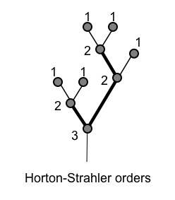
Figure 1. Example of Horton-Strahler ordering. Two order-2 branches are depicted by heavy lines. The branch to the left from the root consists of one vertex; the branch to the right from the root consists of two vertices.

where $\delta_{ij}$ is the Kronecker’s delta. Figure 1 illustrates this definition. A branch is defined as a union of connected vertices with the same order.

2.3. Horton self-similarity

Let ${\mathcal{Q}}_{N}$ be a probability measure on ${\mathcal{T}}_{N}$ and $N_{k}^{({\mathcal{Q}}_{N})}$ be the number of branches of Horton-Strahler order $k$ in a tree generated according to ${\mathcal{Q}}_{N}$.

Definition 1.

We say that a sequence of probability laws $\{{\mathcal{Q}}_{N}\}_{N\in\mathbb{N}}$ has well-defined asymptotic Horton ratios if for each $k\in\mathbb{N}^{+}$, random variables $\left(N_{k}^{({\mathcal{Q}}_{N})}/N\right)$ converge in probability, as $N\rightarrow\infty$, to a constant value ${\mathcal{N}}_{k}$, called the asymptotic ratio of the branches of order $k$.

Horton self-similarity implies that the sequence ${\mathcal{N}}_{k}$ decreases in a geometric fashion as $k$ goes to infinity. In this work we use a particular form of decay described below.

Definition 2.

A sequence $\{{\mathcal{Q}}_{N}\}_{N\in\mathbb{N}}$ of probability laws on ${\mathcal{T}}$ with well-defined asymptotic Horton ratios is said to obey a root-Horton self-similarity law if and only if the following limit exists and is finite and positive: $\lim\limits_{k\rightarrow\infty}\Big{(}{\mathcal{N}}_{k}\Big{)}^{-{1\over k}}=R>0.$ The constant $R$ is called the Horton exponent.

3. Coalescent processes, trees

This section reviews Kingman’s coalescent process with $N$ particles and introduces its tree representation.

3.1. Kingman’s $N$-coalescent process

We start by considering a general finite coalescent process defined by a collision kernel [3, 15, 2]. The process begins with $N$ particles (clusters) of mass one. The cluster formation is governed by a symmetric collision rate kernel $K(i,j)=K(j,i)>0$. Namely, a pair of clusters with masses $i$ and $j$ coalesces at the rate $K(i,j)$, independently of the other pairs, to form a new cluster of mass $i+j$. The process continues until there is a single cluster of mass $N$.

Formally, for a given $N$ consider the space ${\mathcal{P}}_{[N]}$ of partitions of $[N]=\{1,2,\ldots,N\}$. Let $\Pi^{(N)}_{0}$ be the initial partition in singletons, and $\Pi^{(N)}_{t}~{}~{}(t\geq 0)$ be a strong Markov process such that $\Pi^{(N)}_{t}$ transitions from partition $\pi\in{\mathcal{P}}_{[N]}$ to $\pi^{\prime}\in{\mathcal{P}}_{[N]}$ with rate $K(i,j)$ provided that partition $\pi^{\prime}$ is obtained from partition $\pi$ by merging two clusters of $\pi$ of masses $i$ and $j$. If $K(i,j)\equiv 1$ for all positive integer masses $i$ and $j$, the process $\Pi^{(N)}_{t}$ is known as Kingman’s $N$-coalescent process.

3.2. Coalescent tree

A merger history of Kingman’s $N$-coalescent process can be naturally described by a time oriented binary tree $T^{(N)}_{\rm K}$ constructed as follows. Start with $N$ leaves that represent the initial $N$ particles and have time mark $t=0$. When two clusters coalesce (a transition occurs), merge the corresponding vertices to form an internal vertex with a time mark of the coalescent. The final coalescence forms the tree root. The resulting time oriented binary tree represents the history of the process. We notice that a given unlabeled tree corresponds to multiple coalescent trajectories obtained by relabeling of the initial particles.

Observe that the combinatorial version $\textsc{shape}\left(T_{\rm K}^{(N)}\right)$ of the Kingman’s coalescent tree is invariant under time scaling $t_{\rm new}=C\,t_{\rm old}$, $C>0$. Thus without loss of generality we let $K(i,j)\equiv 1/N$ in Kingman’s $N$-coalescent process. Slowing the process’s evolution $N$ times is natural in Smoluchowski coagulation equations that describe the dynamics of the fraction of clusters of different masses.

4. Statement of results

The main result of this paper is root-Horton self-similarity for the combinatorial tree $\textsc{shape}\left(T^{(N)}_{\rm K}\right)$ of the Kingman’s $N$-coalescent process, as $N$ goes to infinity. Specifically, let $N_{k}$ denote the number of branches of Horton-Strahler order $k$ in the tree $T^{(N)}_{\rm K}$ that describes Kingman $N$-coalescent. We show in Sect. 5, Lemma 3 that for each $k\geq 1$, $N_{k}/N$ converges in probability to the asymptotic Horton ratio

$${\mathcal{N}}_{k}=\lim_{N\to\infty}N_{k}/N.$$

Moreover, these ${\mathcal{N}}_{k}$ are finite and can be expressed as

$${\mathcal{N}}_{k}=\frac{1}{2}\int_{0}^{\infty}g_{k}^{2}(x)\,dx,$$

where the sequence $g_{k}(x)$ solves the following system of ordinary differential equations (ODEs):

$$g^{\prime}_{k+1}(x)-{g^{2}_{k}(x)\over 2}+g_{k}(x)g_{k+1}(x)=0,\quad x\geq 0$$

with $g_{1}(x)=2/(x+2)$, $g_{k}(0)=0$ for $k\geq 2$. Equivalently,

$${\mathcal{N}}_{k}=\int_{0}^{1}\left(1-\left(1-x\right)h_{k-1}(x)\right)^{2}dx,$$

where $h_{0}\equiv 0$ and the sequence $h_{k}(x)$ satisfies the ODE system

$$h^{\prime}_{k+1}(x)=2h_{k}(x)h_{k+1}(x)-h_{k}^{2}(x),\quad 0\leq x\leq 1$$

with the initial conditions $h_{k}(0)=1$ for $k\geq 1$.

The root-law Horton self-similarity is proven in Section 6 in the following statement.

Theorem 1.

The asymptotic Horton ratios ${\mathcal{N}}_{k}$ exist and finite and satisfy the convergence $\lim\limits_{k\rightarrow\infty}\left({\mathcal{N}}_{k}\right)^{-{1\over k}}=R$ with $2\leq R\leq 4$.

Numerical solution for the sequence $h_{k}$ provides an estimation of Horton exponent $R=3.043827\ldots$ and suggests that ${\mathcal{N}}_{k}$ also obey a stronger version of Horton self-similarity: $\lim\limits_{k\rightarrow\infty}\left({\mathcal{N}}_{k}\,R^{k}\right)=N_{0}>0$.

Section 7.1 introduces a level set tree $\textsc{level}(X_{i})$ that describes the structure of the level sets of a discrete-time function $X_{i}$, $i=1,\dots,i_{\rm max}$. In particular, we show that there exists a one-to-one map between finite rooted planar time oriented binary trees and sequences of the local extrema of $X_{i}$. Let $W=\{W_{i}\}$ be a discrete white noise, that is a process comprised of i.i.d. values with a common atomless distribution. Consider now a process $\tilde{W}^{(N)}_{i}$ with exactly $N$ local maxima separated by $N-1$ internal local minima such that the latter form a discrete white noise; we call $\tilde{W}^{(N)}_{i}$ an extended discrete white noise.

Let $L^{(N)}_{W}=\textsc{level}\left(\tilde{W}^{(N)}_{i}\right)$ be the level set tree of $\tilde{W}^{(N)}_{i}$ and $\textsc{shape}\left(L^{(N)}_{W}\right)$ be the combinatorial tree that retains the graph-theoretic structure of $L^{(N)}_{W}$ and drops its planar embedding as well as the time marks of the vertices. Furthermore, let $T^{(N)}_{\rm K}$ be the tree that corresponds to a Kingman’s $N$-coalescent, and let $\textsc{shape}\left(T^{(N)}_{\rm K}\right)$ be its combinatorial version that drops the time marks of the vertices. By construction, both the trees $\textsc{shape}\left(L^{(N)}_{W}\right)$ and $\textsc{shape}\left(T^{(N)}_{\rm K}\right)$, belong to the space ${\mathcal{T}}_{N}$ of binary rooted trees with $N$ leaves. Section 7.2 establishes the following equivalence.

Theorem 2.

The trees $\textsc{shape}\left(L^{(N)}_{W}\right)$ and $\textsc{shape}\left(T^{(N)}_{\rm K}\right)$ have the same distribution on ${\mathcal{T}}_{N}$.

The equivalence leads to the Horton self-similarity for discrete white noise.

Corollary 1.

The combinatorial level set tree of a discrete white noise is root-Horton self similar with the same Horton exponent $R$ as for Kingman’s coalescent.

5. Smoluchowski-Horton ODEs for Kingman’s coalescent

Consider Kingman’s $N$-coalescent process and its tree representation $T^{(N)}_{\rm K}$. In Section 5.1 we informally write Smoluchowski-type ODEs for the number of Horton-Strahler branches in the coalescent tree $T^{(N)}_{\rm K}$ and consider the asymptotic version of these equations as $N\to\infty$. Section 5.2 formally establishes the validity of the hydrodynamic limit.

5.1. Main equation

Recall that we let $K(i,j)\equiv 1/N$ in Kingman’s $N$-coalescent process. Let $|\Pi^{(N)}_{t}|$ denote the total number of clusters at time $t\geq 0$, and let $\eta_{(N)}(t):=|\Pi^{(N)}_{t}|/N$ be the total number of clusters relative to the system size $N$. Then $\eta_{(N)}(0)=N/N=1$ and $\eta_{(N)}(t)$ decreases by $1/N$ with each coalescence of clusters with the rate

$${1\over N}\,\binom{N\,\eta_{(N)}(t)}{2}={\eta_{(N)}^{2}(t)\over 2}\cdot N+o(N),\quad{\rm as~{}}N\to\infty,$$

since $1/N$ is the coalescence rate for any pair of clusters regardless of their masses. Informally, this implies that the limit relative number of clusters $\displaystyle\eta(t)=\lim_{N\to\infty}\eta_{(N)}(t)$ satisfies the following ODE:

(1) $${d\over dt}\eta(t)=-\frac{\eta^{2}(t)}{2}.$$

The corresponding initial condition $\eta(0)=1$ implies a unique solution $\eta(t)=2/(2+t)$.

Next, for any $k\in\mathbb{N}^{+}$ we define $\eta_{k,N}(t)$ to be the number of clusters that correspond to branches of Horton-Strahler order $k$ at time $t$ relative to the system size $N$. Initially, each particle represents a leaf of Horton-Strahler order $1$. Accordingly, the initial conditions are set to be, using Kronecker’s delta notation,

$$\eta_{k,N}(0)=\delta_{1}(k).$$

We describe now the evolution of $\eta_{k,N}(t)$ using the definition of Horton-Strahler orders.

Observe that $~{}\eta_{k,N}(t)$ increases by $1/N$ with each coalescence of clusters of Horton-Strahler order $k-1$ that happens with the rate

$${1\over N}\,\binom{N\,\eta_{k-1,N}(t)}{2}={\eta_{k-1,N}^{2}(t)\over 2}\cdot N+o(N).$$

Thus ${\eta_{k-1,N}^{2}(t)\over 2}+o(1)$ is the instantaneous rate of increase of $\eta_{k,N}(t)$.

Similarly, $~{}\eta_{k,N}(t)$ decreases by $1/N$ when a cluster of order $k$ coalesces with a cluster of order strictly higher than $k$ with the rate

$$\eta_{k,N}(t)\,\left(\eta_{(N)}(t)-\sum\limits_{j=1}^{k}\eta_{j,N}(t)\right)\cdot N,$$

and it decreases by $2/N$ when a cluster of order $k$ coalesces with another cluster of order $k$ with the rate

$${1\over N}\,\binom{N\,\eta_{k,N}(t)}{2}={\eta_{k,N}^{2}(t)\over 2}\cdot N+o(N).$$

Thus the instantaneous rate of decrease of $\eta_{k,N}(t)$ is

$$\eta_{k,N}(t)\,\left(\eta_{(N)}(t)-\sum\limits_{j=1}^{k}\eta_{j,N}(t)\right)+\eta^{2}_{k,N}(t)+o(1).$$

Now we can informally write the limit rates-in and the rates-out for the clusters of Horton-Strahler order via the following Smoluchowski-Horton system of ODEs:

(2) $${d\over dt}\eta_{k}(t)=\frac{\eta^{2}_{k-1}(t)}{2}-\eta_{k}(t)\,\left(\eta(t)-\sum\limits_{j=1}^{k-1}\eta_{j}(t)\right)$$

with the initial conditions $\eta_{k}(0)=\delta_{1}(k)$. Here we define $\displaystyle\eta_{k}(t)=\lim_{N\to\infty}\eta_{k,N}(t)$, provided it exists, and let $\eta_{0}\equiv 0$.

Since $\eta_{k}(t)$ has the instantaneous rate of increase ${\eta_{k-1}^{2}(t)\over 2}$, the relative total number of clusters corresponding to branches of Horton-Strahler order $k$ is given by

(3) $${\mathcal{N}}_{k}=\delta_{1}(k)+\int\limits_{0}^{\infty}{\eta^{2}_{k-1}(t)\over 2}dt.$$

It is not hard to compute the first three terms of the sequence ${\mathcal{N}}_{k}$ by solving equations (1) and (2) in the first three iterations:

$${\mathcal{N}}_{1}=1,\quad{\mathcal{N}}_{2}={1\over 3},\quad\text{ and }\quad{\mathcal{N}}_{3}={e^{4}\over 128}-{e^{2}\over 8}+{233\over 384}=0.109686868100941\ldots$$

Hence, we have ${{\mathcal{N}}_{1}/{\mathcal{N}}_{2}}={3}$ and ${{\mathcal{N}}_{2}/{\mathcal{N}}_{3}}=3.038953879388\dots$ Our numerical results yield, moreover,

$$\lim\limits_{k\rightarrow\infty}\left({\mathcal{N}}_{k}\right)^{-{1\over k}}=\lim\limits_{k\rightarrow\infty}{{\mathcal{N}}_{k}\over{\mathcal{N}}_{k+1}}=3.0438279\dots$$

5.2. Hydrodynamic limit

This section establishes the existence of the asymptotic ratios ${\mathcal{N}}_{k}$ as well as the validity of the equations (1), (2) and (3) in a hydrodynamic limit. We refer to Darling and Norris [5] for a survey of formal techniques for proving that a Markov chain converges to the solution of a differential equation.

Notice that quasilinearity of the system of ODEs in (2) implies the existence and uniqueness. Specifically, if the first $k-1$ functions $\eta_{1}(t),\ldots,\eta_{k-1}(t)$ are given, then (2) is a linear equation in $\eta_{k}(t)$. The following argument is different from the one presented by Norris [13] for the Smoluchowski equations.

Lemma 1.

Let $\eta_{(N)}(t)$ be the relative total number of clusters and $\eta(t)$ be the solution to equation (1) with the initial condition $\eta(0)=1$. Then

$$\big{\|}\eta_{(N)}(t)-\eta(t)\big{\|}_{L^{\infty}[0,\infty)}\rightarrow 0$$

in probability as $N\to\infty$.

A proof of Lemma 1 is given in Appendix A. The proof is divided into steps that we briefly outline below.

$\bullet$ Steps I, II. We start by establishing bounds on the number of coalescences within the time interval $[t,t+\delta]$. Specifically, fix $\epsilon_{0}\in(0,1)$ and take $\delta>0$. Given $y\in{1\over N}\mathbb{Z}\cap[\epsilon_{0},1]$, let $u=\binom{Ny}{2}$ and $v=\binom{Ny-\lceil{\delta y^{2}\over 2}N\rceil}{2}$. We use the exponential Markov inequality to show that for any given $t\geq 0$ and large enough $N$ we have

$$P\left({\delta\over N^{2}}v-(1+\delta)N^{-1/3}\leq\eta_{(N)}(t)-\eta_{(N)}(t+\delta)\leq{\delta\over N^{2}}u+N^{-1/3}~{}~{}\Big{|}~{}\eta_{(N)}(t)=y~{}\right)$$

$$\geq\left(1-\exp\left\{-N^{1/6}+{4\delta\over\epsilon_{0}^{2}}\right\}\right)^{2}.$$

$\bullet$ Step III. The bounds of steps I, II are applied to show that

$P\left(~{}\left|{\eta^{2}_{(N)}(t)\over 2}+\Delta_{\delta}\eta_{(N)}(t)\right|~{}\leq~{}\delta+(\delta^{-1}+1)N^{-1/3}~{}~{}\Big{|}~{}\eta_{(N)}(t)=y~{}\right)$

(4) $$\geq\left(1-\exp\left\{-N^{1/6}+{4\delta\over\epsilon_{0}^{2}}\right\}\right)^{2}$$

for $N$ large enough, where $~{}\Delta_{\delta}f(x):={f(x+\delta)-f(x)\over\delta}~{}$ denotes the forward difference.

$\bullet$ Step IV. For $K>0$, consider an interval $[0,K]$ partitioned into $M$ subintervals

$$[t_{0},t_{1}],~{}[t_{1},t_{2}],~{}\ldots,~{}[t_{M-1},t_{M}]$$

of equal length $\delta=K/M$, where $t_{0}=0$ and $t_{M}=K$. Let $\epsilon_{0}=\eta(K)/2=1/(2+K)$, where $\eta(t)=2/(2+t)$ is the solution to the equation (1) with the initial condition $\eta(0)=1$. Consider the difference equation

(5) $$\Delta_{\delta}\psi_{(N)}(t_{i})=-{\psi_{(N)}^{2}(t_{i})\over 2}+\mathcal{E}^{\prime}(t_{i})$$

with initial condition $\psi_{(N)}(0)=1$, where the error $~{}|\mathcal{E}^{\prime}(t_{i})|\leq\delta+(\delta^{-1}+1)N^{-1/3}$. At this step we prove that if $M$ is large enough and for any natural number $j\leq M$ function $\psi_{(N)}(t_{i})$ satisfies (5) for all $i\in\{0,1,\ldots,j-1\}$, then

$$\psi_{(N)}(t_{j})\geq\epsilon_{0}$$

as we take $N$ large enough. This follows from observing that $\eta(t)$ will satisfy a difference equation similar to (5),

(6) $$\Delta_{\delta}\eta(t_{i})=-{\eta^{2}(t_{i})\over 2}+\mathcal{E}(t_{i})$$

with $~{}|\mathcal{E}(t_{i})|\leq{1\over 4}\delta~{}$ for all $i\in\{0,1,\ldots,M-1\}$.

$\bullet$ Step V. Consider events

(7) $$A_{i}=\left\{~{}\Delta_{\delta}\eta_{(N)}(t_{i})=-{\eta^{2}_{(N)}(t_{i})\over 2}+\mathcal{E}^{\prime}(t_{i})~{}\text{ and }~{}|\mathcal{E}^{\prime}(t_{i})|~{}\leq\delta+(\delta^{-1}+1)N^{-1/3}~{}\right\}$$

for all $i\in\{0,1,\ldots,M-1\}$. Here we combine the results of steps III and IV and establish that with probability greater than $P\left(~{}\bigcap\limits_{i=0}^{M-1}A_{i}~{}\right)\rightarrow 1$ as $M\rightarrow\infty$, $~{}\eta_{(N)}(t_{i})$ satisfies the difference equation (5) with $\psi_{(N)}(t)\equiv\eta_{(N)}(t)$.

$\bullet$ Step VI. Taking $\psi_{(N)}(t)\equiv\eta_{(N)}(t)$, we compare the difference equation (5) with (6), and bound the error $|\eta_{(N)}(t)-\eta(t)|$ for all $t\in[0,K]$. Specifically, we show that with probability greater than $~{}P\left(~{}\bigcap\limits_{i=0}^{M-1}A_{i}~{}\right)\rightarrow 1$,

(8) $$\big{\|}\eta_{(N)}(t)-\eta(t)\big{\|}_{L^{\infty}[0,K]}\leq{15\over 4}K^{2}/M+4K/M+3/M$$

for $M$ large enough and $N\geq M^{6}$. Therefore, letting $M\rightarrow\infty$, we obtain

$$\big{\|}\eta_{(N)}(t)-\eta(t)\big{\|}_{L^{\infty}[0,K]}\rightarrow 0\qquad\text{ in probability.}$$

$\bullet$ Step VII. Take $\epsilon\in(0,1)$ and $\gamma>1$, and consider $K>{2(1-\epsilon)\over\epsilon}\gamma$. This step uses Markov inequality to show that

$$P\Big{(}\big{\|}\eta_{(N)}(t)-\eta(t)\big{\|}_{L^{\infty}[K,\infty)}<\epsilon\Big{)}~{}>1-1/\gamma,$$

which, together with the results of step VI, implies

$$\limsup\limits_{N\rightarrow\infty}P\Big{(}\big{\|}\eta_{(N)}(t)-\eta(t)\big{\|}_{L^{\infty}[0,\infty)}<\epsilon\Big{)}\geq 1-1/\gamma.$$

We conclude that

$$\lim\limits_{N\rightarrow\infty}P\Big{(}\big{\|}\eta_{(N)}(t)-\eta(t)\big{\|}_{L^{\infty}[0,\infty)}<\epsilon\Big{)}=1.$$

Therefore we have shown that $~{}\|\eta_{(N)}(t)-\eta(t)\|_{L^{\infty}[0,\infty)}\rightarrow 0~{}$ in probability, thus establishing Lemma 1.

We now proceed with establishing a hydrodynamic limit for the Smoluchowski-Horton system of ODEs (2). Let

$$\eta_{k,N}(t):={N_{k}(t)\over N}~{}~{}~{}\text{ and }~{}~{}~{}g_{k,N}(t):=\eta_{(N)}(t)-\sum\limits_{j:j<k}\eta_{j,N}(t).$$

Lemma 2.

Consider the relative numbers $\eta_{k,N}(t)$ of clusters that correspond to branches of Horton-Strahler order $k$ and functions $\eta_{k}(t)$ that solve the system of equations (2) with the initial conditions $\eta_{k}(0)=\delta_{1}(k)$. Then,

$$\|\eta_{k,N}(t)-\eta_{k}(t)\|_{L^{\infty}[0,\infty)}\rightarrow 0,\quad\forall k\geq 1,$$

in probability, as $N\to\infty$.

A proof of Lemma 2 is given in Appendix B. Here we summarize the steps used in the proof.

$\bullet$ Step I. We use the setting from the proof of Lemma 1. Fix $K>0$ and consider an interval $[0,K]$ partitioned into $M$ subintervals

$$[t_{0},t_{1}],~{}[t_{1},t_{2}],~{}\ldots,~{}[t_{M-1},t_{M}]$$

of equal length $\delta=K/M$, where $t_{0}=0$ and $t_{M}=K$. Let $\epsilon_{0}=\eta(K)/2=1/(2+K)$. The total number of coalescences within the interval $[t_{i},t_{i+1}]$ equals $N\big{[}\eta_{(N)}(t_{i})-\eta_{(N)}(t_{i+1})\big{]}$.

For any $k\in\mathbb{N}^{+}$ and any $i=0,1,\ldots,M-1$ we represent the relative number of coalescences that involve the clusters of order $k$ within $[t_{i},t_{i+1}]$ as

$$\eta_{k,N}(t_{i+1})-\eta_{k,N}(t_{i})=\xi_{1}+\xi_{2}+\ldots+\xi_{m_{i}},$$

where $~{}\xi_{1},\xi_{2},\ldots,\xi_{m_{i}}~{}$ are random variables that correspond to the $m_{i}$ coalescences (of any Horton-Strahler order) within $[t_{i},t_{i+1}]$ in the order of occurrence. Here, each $\xi_{r}$ can take values in $\frac{1}{N}\{-2,-1,0,1\}$; and their dependence on $k$ is omitted to simplify the notations. By construction, conditioned on the values $\{\eta_{j,N}(t_{i})\}_{j}$, the distribution of $\xi_{r}$ for $1\leq r\leq m_{i}$ is completely determined by the history $~{}\mathcal{T}_{r-1}$ of the preceding $r-1$ transitions.

Consider a random variable $\xi$ with the values $\{-2,-1,0,1\}$ specified by the probabilities $\{p(-2),p(-1),p(0),p(1)\}$:

$$p(-2) := \eta^{2}_{k,N}(t_{i})/\eta^{2}_{(N)}(t_{i}),$$

$$p(1) := \begin{cases}\eta^{2}_{k-1,N}(t_{i})/\eta^{2}_{(N)}(t_{i})&\text{ if }k>1\\ 0&\text{ if }k=1\end{cases},$$

$$p(-1) := 2\eta_{k,N}(t_{i})g_{k+1,N}(t_{i})/\eta^{2}_{(N)}(t_{i}),$$

$$p(0) := 1-p(-2)-p(-1)-p(1).$$

Recall the events $A_{i}$ defined in (7). We notice that, conditioned on $\bigcap\limits_{i^{\prime}=0}^{i}A_{i^{\prime}}$, the total variation distance between the distribution of $\xi_{r}$ (for a fixed $1\leq r\leq m_{i}$) and the distribution of $\xi$ is of order $\mathcal{O}(\delta)$. We use this to show that for each $k\in\mathbb{N}^{+}$, there is a large enough $c_{k}>0$ and $a>0$ such that

(9) $$P\Big{(}\Big{|}\big{[}\eta_{k,N}(t_{i+1})-\eta_{k,N}(t_{i})\big{]} - E[\xi]\delta{\eta^{2}_{(N)}(t_{i})\over 2}\Big{|}<c_{k}\delta^{4/3}~{}\Big{|}~{}\bigcap\limits_{i^{\prime}=0}^{i}A_{i^{\prime}}~{}\Big{)}$$

$$\geq 1-\exp\Big{\{}-aM^{4}\Big{\}}$$

for all $i=0,1,\ldots,M-1$, $~{}2M^{6}>N>M^{6}$, and $M$ large enough.

$\bullet$ Step II. According to the results of step I, we obtain the following system of difference equations:

$$\Delta_{\delta}\eta_{1,N}(t_{i}) = -\eta_{1,N}(t_{i})\eta_{(N)}(t_{i})+\mathcal{E}^{\prime}_{1}(t_{i})$$

$$\Delta_{\delta}\eta_{k,N}(t_{i}) = {\eta^{2}_{k-1,N}(t_{i})\over 2}-\eta_{k,N}(t_{i})g_{k,N}(t_{i})+\mathcal{E}^{\prime}_{k}(t_{i})\quad\text{ for }k\geq 2$$

with the initial conditions

$$\Big{(}\eta_{1,N}(0),~{}\eta_{2,N}(0),~{}\ldots,~{}\eta_{k,N}(0),~{}\ldots\Big{)}=(1,0,0,\ldots),$$

where for a given $\rho\in\mathbb{N}$ and $c=\max\limits_{1\leq k\leq\rho}\{c_{k}\}$ we have $|\mathcal{E}^{\prime}_{k}(t_{i})|<c\delta^{1/3}$ for each $1\leq k\leq\rho$. Each equation in this system holds with the probability that converges to unity as $M$ increases.

We now compare the above difference equations (5.2) to the following system of difference equations that corresponds to the system of ODEs (2):

$$\Delta_{\delta}\eta_{1}(t_{i}) = -\eta_{1}(t_{i})\eta(t_{i})+\mathcal{E}_{1}(t_{i})$$

$$\Delta_{\delta}\eta_{k}(t_{i}) = {\eta^{2}_{k-1}(t_{i})\over 2}-\eta_{k}(t_{i})g_{k}(t_{i})+\mathcal{E}_{k}(t_{i})\quad\text{ for }k\geq 2,$$

where $~{}g_{k}(t):=\eta(t)-\sum\limits_{i:~{}i<k}\eta_{i}(t)$, and the error

$$\mathcal{E}_{k}(t_{i})={\eta^{\prime\prime}_{k}(c_{i,k})\over 2}\delta\qquad\text{ for some }c_{i,k}\in(t_{i},t_{i+1}).$$

$\bullet$ Step III. We show that, conditioning on the event $~{}\bigcap\limits_{i=0}^{M-1}A_{i}$, we have the following upper bound for any $k\in\{1,\ldots,\rho\}$, all $i\in\{0,1,\ldots,M-1\}$, and $t\in(t_{i},t_{i+1})$:

$$\big{|}\eta_{k,N}(t)-\eta_{k}(t)\big{|} \leq \big{|}\eta_{k,N}(t)-\eta_{k,N}(t_{i})\big{|}+\big{|}\eta_{k,N}(t_{i})-\eta_{k}(t_{i})\big{|}+\big{|}\eta_{k}(t_{i})-\eta_{k}(t)\big{|}$$

$$\leq \left(5K^{2}+4K+4\right)/M+(c+1)2^{k}{\delta^{1/3}\over\rho}\big{[}e^{2K\rho}-1\big{]}+3\delta.$$

We conclude that, for any $k$,

$$\|\eta_{k,N}-\eta_{k}\|_{L^{\infty}[0,K]}\rightarrow 0\quad\text{in probability}.$$

$\bullet$ Step IV. Finally, observe that for any $\epsilon>0$ and for $K>2$ large enough so that $~{}\eta(K)<\epsilon$,

$$\eta_{k}(t)\leq\eta(t)\leq\eta(K)<\epsilon\text{ for all }t\geq K$$

and

$$P\Big{(}\big{\|}\eta_{k,N}(t)-\eta_{k}(t)\big{\|}_{L^{\infty}[K,\infty)}>\epsilon\Big{)} \leq P\Big{(}\big{\|}\eta_{k,N}(t)\big{\|}_{L^{\infty}[K,\infty)}>\epsilon\Big{)}$$

$$\leq P\Big{(}\big{\|}\eta_{(N)}(t)\big{\|}_{L^{\infty}[K,\infty)}>\epsilon\Big{)}$$

$$= P\Big{(}\eta_{(N)}(K)>\epsilon\Big{)}$$

$$\leq {2(1-\epsilon)\over\epsilon K}.$$

The last bound is obtained from Markov inequality for the random variable $T_{m}$ that represents the time of the $m$-th coalescence. Therefore, together with the result of the previous step, we have shown that for each $k$,

$$\|\eta_{k,N}-\eta_{k}\|_{L^{\infty}[0,\infty)}\rightarrow 0$$

in probability. This completes the proof.

Finally, the last lemma in this section establishes a hydrodynamic limit for the Horton ratios.

Lemma 3.

The Horton ratios $~{}N_{k}/N~{}$ converge in probability to a finite constant ${\mathcal{N}}_{k}$ given by (3), as $~{}N\rightarrow\infty$.

A proof of Lemma 3 is given in Appendix C.

6. The root-Horton self-similarity and related results

We begin this section with preliminary lemmas and propositions, and then proceed to proving Theorem 1.

Let $g_{1}(t)=\eta(t)$ and $g_{k}(t)=\eta(t)-\sum\limits_{j:~{}j<k}\eta_{j}(t)$ be the asymptotic number of clusters of Horton order $k$ or higher at time $t$. We can rewrite (2) via $g_{k}$ using $\eta_{k}(t)=g_{k}(t)-g_{k+1}(t)$:

$${d\over dt}g_{k}(t)-{d\over dt}g_{k+1}(t)={\big{(}g_{k-1}(t)-g_{k}(t)\big{)}^{2}\over 2}-(g_{k}(t)-g_{k+1}(t))g_{k}(t).$$

Observe that $g_{1}(t)\geq g_{2}(t)\geq g_{3}(t)\geq\ldots$. We now rearrange the terms, obtaining for all $k\geq 2$,

(12) $$~{}~{}~{}~{}~{}~{}{d\over dt}g_{k+1}(t)-{g^{2}_{k}(t)\over 2}+g_{k}(t)g_{k+1}(t)={d\over dt}g_{k}(t)-{g^{2}_{k-1}(t)\over 2}+g_{k-1}(t)g_{k}(t).$$

One can readily check that ${d\over dt}g_{2}(t)-{g^{2}_{1}(t)\over 2}+g_{1}(t)\,g_{2}(t)=0$; the above equations hence simplify as follows

(13) $$g^{\prime}_{k+1}(t)-{g^{2}_{k}(t)\over 2}+g_{k}(t)g_{k+1}(t)=0\qquad$$

$$\text{ with }~{}g_{1}(t)={2\over t+2},\text{ and }g_{k}(0)=0\text{ for }k\geq 2.$$

Next, returning to the asymptotic ratios of the number of order-$k$ branches to $N$, we observe that (12) implies that, for $k\geq 2$,

$${\mathcal{N}}_{k}=\int\limits_{0}^{\infty}{\eta^{2}_{k-1}(t)\over 2}dt=\int\limits_{0}^{\infty}{(g_{k-1}(t)-g_{k}(t))^{2}\over 2}dt=\int\limits_{0}^{\infty}{g^{2}_{k}(t)\over 2}dt$$

since

$${(g_{k-1}(t)-g_{k}(t))^{2}\over 2}={d\over dt}g_{k}(t)+{g^{2}_{k}(t)\over 2},$$

where $\int\limits_{0}^{\infty}{d\over dt}g_{k}(t)dt=g_{k}(\infty)-g_{k}(0)=0$ for $k\geq 2$. Let $n_{k}$ represent the number of order-$k$ branches relative to the number of order-$(k+1)$ branches:

$$n_{k}:={{\mathcal{N}}_{k}\over{\mathcal{N}}_{k+1}}={\frac{1}{2}\int\limits_{0}^{\infty}{g^{2}_{k}(t)}dt\over\frac{1}{2}\int\limits_{0}^{\infty}{g^{2}_{k+1}(t)}dt}={\|g_{k}\|^{2}_{L^{2}[0,\infty)}\over\|g_{k+1}\|^{2}_{L^{2}[0,\infty)}}.$$

Consider the following limits that represent respectively the root and the ratio asymptotic Horton laws:

$$\lim\limits_{k\rightarrow\infty}\left({\mathcal{N}}_{k}\right)^{-{1\over k}}=\lim\limits_{k\rightarrow\infty}\left(\prod\limits_{j=1}^{k}n_{j}\right)^{-{1\over k}}\qquad\text{ and }\qquad\lim\limits_{k\rightarrow\infty}n_{k}=\lim\limits_{k\rightarrow\infty}{\|g_{k}\|^{2}_{L^{2}[0,\infty)}\over\|g_{k+1}\|^{2}_{L^{2}[0,\infty)}}.$$

Theorem 1 establishes the existence of the first limit. We expect the second, stronger, limit also to exist and both of them to be equal to $3.043827\dots$ according to our numerical results. We now establish some basic facts about $g_{k}$ and $n_{k}$.

Proposition 1.

Let $g_{k}(x)$ solve the ODE system (13). Then

  (a):

$~{}\frac{1}{2}\int\limits_{0}^{\infty}{g^{2}_{k}(t)}dt=\int\limits_{0}^{\infty}g_{k}(t)g_{k+1}(t)dt,$

  (b):

$~{}\int\limits_{0}^{\infty}g^{2}_{k+1}(t)dt=\int\limits_{0}^{\infty}(g_{k}(t)-g_{k+1}(t))^{2}dt,$

  (c):

$~{}\lim\limits_{t\rightarrow\infty}tg_{k}(t)=2,$

  (d):

$~{}n_{k}={\|g_{k}\|^{2}_{L^{2}[0,\infty)}\over\|g_{k+1}\|^{2}_{L^{2}[0,\infty)}}\geq{2},$

  (e):

$~{}n_{k}={\|g_{k}\|^{2}_{L^{2}[0,\infty)}\over\|g_{k+1}\|^{2}_{L^{2}[0,\infty)}}\leq{4}.$

Proof.

Part (a) follows from integrating (13), and part (b) follows from part (a). Part (c) is done by induction, using the L’Hôpital’s rule as follows. It is obvious that $~{}\lim\limits_{x\rightarrow\infty}tg_{1}(t)=2$. We observed earlier that $g_{1}(t)\geq g_{2}(t)\geq g_{3}(t)\geq\ldots$. Hence, for any $k\geq 1$,

$$tg_{k}(t)\leq tg_{1}(t)={2t\over t+2}<2\quad\forall t\geq 0.$$

Also,

$$[tg_{k+1}]^{\prime}={tg^{2}_{k}(t)\over 2}-tg_{k}(t)g_{k+1}(t)+g_{k+1}(t)={\big{(}g_{k}(t)-g_{k+1}(t)\big{)}tg_{k}(t)+\big{(}2-tg_{k}(t)\big{)}g_{k+1}(t)\over 2}$$

implying $~{}[tg_{k+1}]^{\prime}\geq 0~{}$ for all $t\geq 0$ as $g_{k}(t)-g_{k+1}(t)\geq 0$ and $2-tg_{k}(t)>0$. Hence, $tg_{k+1}(t)$ is bounded and nondecreasing. Thus, $~{}\lim\limits_{t\rightarrow\infty}tg_{k+1}(t)$ exists for all $k\geq 1$.

Next, suppose $~{}\lim\limits_{t\rightarrow\infty}tg_{k}(t)=2$. Then by the Mean Value Theorem, for any $t>0$ and for all $y>t$,

$${g_{k+1}(t)-g_{k+1}(y)\over t^{-1}-y^{-1}}\leq\sup\limits_{z:~{}z\geq t}{g^{\prime}_{k+1}(z)\over-z^{-2}}.$$

Taking $~{}y\rightarrow\infty$, obtain

$${g_{k+1}(t)\over t^{-1}}\leq\sup\limits_{z:~{}z\geq t}{g^{\prime}_{k+1}(z)\over-z^{-2}}.$$

Therefore

$$\lim\limits_{t\rightarrow\infty}tg_{k+1}(t)=\lim\limits_{t\rightarrow\infty}{g_{k+1}(t)\over t^{-1}}=\limsup\limits_{z\rightarrow\infty}{g^{\prime}_{k+1}(z)\over-z^{-2}}=\limsup\limits_{z\rightarrow\infty}{{g^{2}_{k}(z)\over 2}-g_{k}(z)g_{k+1}(z)\over-z^{-2}}$$

$$=\limsup\limits_{z\rightarrow\infty}\left[z^{2}g_{k}(z)g_{k+1}(z)-{z^{2}g^{2}_{k}(z)\over 2}\right]=2\lim\limits_{t\rightarrow\infty}tg_{k+1}(t)-2$$

implying $~{}\lim\limits_{t\rightarrow\infty}tg_{k+1}(t)=2$. The statement (d) follows from the tree construction process. An alternative proof of (d) using differential equations is given in the following subsection. Part (e) follows from part (a) together with Hölder inequality

$${1\over 2}\|g_{k}\|^{2}_{L^{2}[0,\infty)}=\int\limits_{0}^{\infty}g_{k}(t)g_{k+1}(t)dt\leq\|g_{k}\|_{L^{2}[0,\infty)}\cdot\|g_{k+1}\|_{L^{2}[0,\infty)},$$

which implies ${\|g_{k}\|^{2}_{L^{2}[0,\infty)}\over\|g_{k+1}\|^{2}_{L^{2}[0,\infty)}}\leq{4}$. ∎

Finally, observe that $g_{k}(t)\rightarrow 0$ as $k\rightarrow\infty$. Indeed, Proposition 1 and the Dominated Convergence Theorem imply

$$\int\limits_{0}^{\infty}g^{2}_{k+1}(t)dt=\int\limits_{0}^{\infty}(g_{k}(t)-g_{k+1}(t))^{2}dt\rightarrow 0~{}~{}\text{ as }k\rightarrow\infty.$$

Next, following (13),

$$g_{k+1}(t)=\int\limits_{0}^{t}g^{\prime}_{k+1}(y)dy=\int\limits_{0}^{t}{g^{2}_{k}(y)\over 2}dy-\int\limits_{0}^{t}g_{k}(y)g_{k+1}(y)dy\rightarrow 0~{}~{}\text{ as }k\rightarrow\infty.$$

6.1. Rescaling to $[0,1]$ interval

Let

$$h_{k}(x)=(1-x)^{-1}-(1-x)^{-2}g_{k+1}\left({2x\over 1-x}\right)$$

for $x\in[0,1]$. Then $h_{0}\equiv 0$, $h_{1}\equiv 1$, and the system of ODEs (13) rewrites as

(14) $$h^{\prime}_{k+1}(x)=2h_{k}(x)h_{k+1}(x)-h_{k}^{2}(x)$$

with the initial conditions $h_{k}(0)=1$.

Observe that the above quasilinearized system of ODEs (14) has $h_{k}(x)$ converging to $h(x)={1\over 1-x}$ as $k\rightarrow\infty$, where $h(x)$ is the solution to Riccati equation $h^{\prime}(x)=h^{2}(x)$ over $[0,1)$, with the initial value $h(0)=1$. Specifically, we have proven that $g_{k}(x)\rightarrow 0$ as $k\rightarrow\infty$. Thus

$$h_{k}(x)=(1-x)^{-1}-(1-x)^{-2}g_{k+1}\left({2x\over 1-x}\right)~{}\rightarrow~{}h(x)={1\over 1-x}.$$

Here the quantity $n_{k}$ rewrites in terms of $h_{k}$ as follows

$$n_{k}={\big{\|}1-h_{k+1}/h\big{\|}^{2}_{L^{2}[0,1]}\over\big{\|}1-h_{k}/h\big{\|}^{2}_{L^{2}[0,1]}}.$$

Observe that $h_{2}(x)=(1+e^{2x})/2$, but for $k\geq 3$ finding a closed form expression becomes increasingly hard. Given $h_{k}(x)$, Eq. (14) is a linear first-order ODE in $h_{k+1}(x)$; its solution is given by $h_{k+1}(x)=\mathcal{H}h_{k}(x)$ with

(15) $$\mathcal{H}f(x)=\left[1-\int_{0}^{x}f^{2}(y)e^{-2\int\limits_{0}^{y}f(s)ds}dy\right]\cdot e^{2\int\limits_{0}^{x}f(s)ds}.$$

Hence, the problem we are dealing with concerns the asymptotic behavior of an iterated non-linear functional.

Using the setting of (14), we give an ODE proof to Proposition 1(d). To do so, we first need to prove the following lemma.

Lemma 4.

$$\big{\|}1-h_{k+1}/h\big{\|}_{L^{2}[0,1]}=\big{\|}h_{k+1}/h-h_{k}/h\big{\|}_{L^{2}[0,1]}$$

Proof.

Observe that

$$h^{\prime}_{k+1}(x)+(h_{k+1}(x)-h_{k}(x))^{2}=h_{k+1}^{2}(x).$$

We now use integration by parts to obtain

$$\int\limits_{0}^{1}{(h_{k+1}(x)-h_{k}(x))^{2}\over h^{2}(x)}dx=\int\limits_{0}^{1}{h_{k+1}^{2}(x)\over h^{2}(x)}dx-\int\limits_{0}^{1}{h^{\prime}_{k+1}(x)\over h^{2}(x)}dx$$

$$=\int\limits_{0}^{1}{h_{k+1}^{2}(x)\over h^{2}(x)}dx+1-2\int\limits_{0}^{1}{h_{k+1}(x)\over h(x)}dx$$

$$=\int\limits_{0}^{1}{(1-h_{k+1}(x))^{2}\over h^{2}(x)}dx$$

since $1/h(x)=1-x$. ∎

Alternative proof of Proposition 1(d).

Notice that $h\geq\dots\geq h_{k+1}\geq h_{k}\geq\dots\geq h_{0}\equiv 0$, which follows from $g_{1}(t)\geq g_{2}(t)\geq g_{3}(t)\geq\dots$ The Lemma 4 implies

$$\big{\|}1-h_{k+1}/h\big{\|}_{L^{2}[0,1]}^{2}=\big{\|}h_{k+1}/h-h_{k}/h\big{\|}_{L^{2}[0,1]}^{2}=\int\limits_{0}^{1}\left[(1-h_{k}/h)-(1-h_{k+1}/h)\right]^{2}dx$$

$$=\big{\|}1-h_{k+1}/h\big{\|}_{L^{2}[0,1]}^{2}+\big{\|}1-h_{k}/h\big{\|}_{L^{2}[0,1]}^{2}-2\int\limits_{0}^{1}(1-h_{k}/h)(1-h_{k+1}/h)dx$$

and therefore

$$\big{\|}1-h_{k}/h\big{\|}_{L^{2}[0,1]}^{2}=2\int\limits_{0}^{1}(1-h_{k}/h)(1-h_{k+1}/h)dx$$

$$=2\big{\|}1-h_{k+1}/h\big{\|}_{L^{2}[0,1]}^{2}+2\int\limits_{0}^{1}(h_{k+1}/h-h_{k}/h)(1-h_{k+1}/h)dx\geq 2\big{\|}1-h_{k+1}/h\big{\|}_{L^{2}[0,1]}^{2}$$

yielding $2\leq{\big{\|}1-h_{k}/h\big{\|}_{L^{2}[0,1]}^{2}\over\big{\|}1-h_{k+1}/h\big{\|}_{L^{2}[0,1]}^{2}}=n_{k}~{}$ as in Proposition 1(d). ∎

It is also true that one can improve Proposition 1(d) to make it a strict inequality since one can check that

$$h(x)>\dots>h_{k+1}(x)>h_{k}(x)>\dots>h_{0}(x)\equiv 0\quad\text{ for }x\in(0,1).$$

6.2. Proof of the existence of the root-Horton limit

Here we present the proof of our main Theorem 1. It is based on Lemma 5 and Lemma 6 that will be proven in the following two subsections.

Lemma 5.

If the limit $\lim\limits_{k\rightarrow\infty}{h_{k+1}(1)\over h_{k}(1)}$ exists, then $\lim\limits_{k\rightarrow\infty}\left({\mathcal{N}}_{k}\right)^{-{1\over k}}=\lim\limits_{k\rightarrow\infty}\left(\prod\limits_{j=1}^{k}n_{j}\right)^{-{1\over k}}$ also exists, and

$$\lim\limits_{k\rightarrow\infty}\left({\mathcal{N}}_{k}\right)^{-{1\over k}}=\lim\limits_{k\rightarrow+\infty}\left({1\over h_{k}(1)}\right)^{-{1\over k}}=\lim\limits_{k\rightarrow\infty}{h_{k+1}(1)\over h_{k}(1)}.$$

Lemma 6.

The limit $\lim\limits_{k\rightarrow\infty}{h_{k+1}(1)\over h_{k}(1)}\geq 1$ exists, and is finite.

Theorem 1.

The limit $\lim\limits_{k\rightarrow\infty}\left({\mathcal{N}}_{k}\right)^{-{1\over k}}=\lim\limits_{k\rightarrow\infty}\left(\prod\limits_{j=1}^{k}n_{j}\right)^{-{1\over k}}=R$ exists. Moreover, $R=\lim\limits_{k\rightarrow\infty}{h_{k+1}(1)\over h_{k}(1)}$, and $2\leq R\leq 4$.

Proof.

The existence and finiteness of $\lim\limits_{k\rightarrow\infty}{h_{k+1}(1)\over h_{k}(1)}$ established in Lemma 6 is the precondition for Lemma 5 that in turn implies the existence and finiteness of the limit $\lim\limits_{k\rightarrow\infty}\left({\mathcal{N}}_{k}\right)^{-{1\over k}}$ as needed for the root-Horton law. Finally, $2\leq R\leq 4$ follows from Proposition 1. ∎

6.3. Proof of Lemma 5 and related results

Proposition 2.

$$\big{\|}1-h_{k+1}(x)/h(x)\big{\|}_{L^{2}[0,1]}^{2}\leq{1\over h_{k+1}(1)}\leq\big{\|}1-h_{k}(x)/h(x)\big{\|}_{L^{2}[0,1]}^{2}.$$

Proof.

Integrating from 0 to 1 both sides of the equation

$${h^{\prime}_{k+1}(x)\over h_{k+1}^{2}(x)}=1-{(h_{k+1}(x)-h_{k}(x))^{2}\over h_{k+1}^{2}(x)}$$

we obtain $~{}{1\over h_{k+1}(1)}=\int\limits_{0}^{1}{(h_{k+1}(x)-h_{k}(x))^{2}\over h_{k+1}^{2}(x)}dx~{}$ as $h_{k+1}(0)=1$.

Hence,

$${1\over h_{k+1}(1)}=\int\limits_{0}^{1}{(h_{k+1}(x)-h_{k}(x))^{2}\over h_{k+1}^{2}(x)}dx\geq\int\limits_{0}^{1}{(h_{k+1}(x)-h_{k}(x))^{2}\over h^{2}(x)}dx=\int\limits_{0}^{1}\left(1-{h_{k+1}(x)\over h(x)}\right)^{2}dx$$

by Lemma 4, proving the first inequality.

Now,

$${1\over h_{k+1}(1)}=\big{\|}1-h_{k}(x)/h_{k+1}(x)\big{\|}_{L^{2}[0,1]}^{2}\leq\big{\|}1-h_{k}(x)/h(x)\big{\|}_{L^{2}[0,1]}^{2}$$

thus completing the proof. ∎

Proof of Lemma 5.

If the limit $\lim\limits_{k\rightarrow\infty}{h_{k+1}(1)\over h_{k}(1)}$ exists and is finite, then $\lim\limits_{k\rightarrow\infty}\left({1\over h_{k}(1)}\right)^{-{1\over k}}$ must also exist and be finite. Hence the existence and finiteness of

$$\lim\limits_{k\rightarrow\infty}\left({\mathcal{N}}_{k}\right)^{-{1\over k}}=\lim\limits_{k\rightarrow\infty}\left(\int_{0}^{1}\left(1-{h_{k}(x)\over h(x)}\right)^{2}dx\right)^{-{1\over k}}$$

follows from Proposition 2. ∎

6.4. Proof of Lemma 6 and related results

In this subsection we use the approach developed by Drmota [8] to prove the existence and finiteness of $\lim\limits_{k\rightarrow\infty}{h_{k+1}(1)\over h_{k}(1)}\geq 1$. As we observed earlier this result is needed to prove the existence, finiteness, and positivity of $\lim\limits_{k\rightarrow\infty}\left({\mathcal{N}}_{k}\right)^{-{1\over k}}=\lim\limits_{k\rightarrow\infty}\left(\prod\limits_{j=1}^{k}n_{j}\right)^{-{1\over k}}$, the root-Horton law.

Definition 3.

Given $\gamma\in(0,1]$. Let

$$V_{k,\gamma}(x)=\begin{cases}{1\over 1-x}&\text{ for }0\leq x\leq 1-\gamma,\\ \gamma^{-1}h_{k}\left({x-(1-\gamma)\over\gamma}\right)&\text{ for }1-\gamma\leq x\leq 1.\end{cases}$$

Note that sequences of functions $h_{k}(x)$ and $V_{k,\gamma}(x)$ can be extended beyond $x=1$.

Here are some observations we make about the above defined functions.

Observation 1.

$V_{k,\gamma}(x)$ are positive continuous functions satisfying

$$V^{\prime}_{k+1,\gamma}(x)=2V_{k+1,\gamma}(x)V_{k,\gamma}(x)-V^{2}_{k,\gamma}(x)$$

for all $x\in[0,1]\setminus(1-\gamma)$, with initial conditions $V_{k,\gamma}(0)=1$.

Observation 2.

Let $\gamma_{k}={h_{k}(1)\over h_{k+1}(1)}$. Then

(16) $$V_{k,\gamma_{k}}(1)=h_{k+1}(1)$$

and

(17) $$V_{k,\gamma}(1)=\gamma^{-1}h_{k}(1)\geq h_{k+1}(1)\quad\text{ whenever }\gamma\leq\gamma_{k}.$$

Observation 3.

$$V_{k,\gamma}(x)\leq V_{k+1,\gamma}(x)$$

for all $x\in[0,1]$ since $h_{k}(x)\leq h_{k+1}(x)$.

Observation 4.

Since $h_{1}(x)\equiv 1$ and $\gamma_{1}={h_{1}(1)\over h_{2}(1)}$,

$$h_{2}(x)\leq V_{1,\gamma_{1}}(x)=\begin{cases}{1\over 1-x}&\text{ for }0\leq x\leq 1-\gamma_{1},\\ \gamma_{1}^{-1}=h_{2}(1)&\text{ for }1-\gamma_{1}\leq x\leq 1.\end{cases}$$

The above observation generalizes as follows.

Proposition 3.

$$h_{k+1}(x)\leq V_{k,\gamma_{k}}(x)=\begin{cases}{1\over 1-x}&{\rm~{}for~{}}0\leq x\leq 1-\gamma_{k},\\ \gamma_{k}^{-1}h_{k}\left({x-(1-\gamma_{k})\over\gamma_{k}}\right)&{\rm~{}for~{}}1-\gamma_{k}\leq x\leq 1.\end{cases}$$

In order to prove Proposition 3 we will need the following lemma.

Lemma 7.

For any $\gamma\in(0,1)$ and $k\geq 1$, function $V_{k,\gamma}(x)-h_{k+1}(x)$ changes its sign at most once as $x$ increases from $1-\gamma$ to $1$. Moreover, since $V_{k,\gamma}(1-\gamma)=h(1-\gamma)>h_{k+1}(1-\gamma)$, function $V_{k,\gamma}(x)-h_{k+1}(x)$ can only change sign from nonnegative to negative.

Proof.

This is a proof by induction with base at $k=1$. Here $V_{1,\gamma}(x)={1\over\gamma}$ is constant on $[1-\gamma,1]$, while $h_{2}(x)=(1+e^{2x})/2$ is an increasing function, and

$$V_{1,\gamma}(1-\gamma)=h(1-\gamma)>h_{2}(1-\gamma)$$

For the induction step, we need to show that if $V_{k,\gamma}(x)-h_{k+1}(x)$ changes its sign at most once, then so does $V_{k+1,\gamma}(x)-h_{k+2}(x)$. Since both sequences of functions satisfy the same ODE relation (see Observation 1), we have

${d\over dx}\left[(V_{k+1,\gamma}(x)-h_{k+2}(x))\cdot e^{-2\int\limits_{1-\gamma}^{x}h_{k+1}(y)dy}\right]$

$$\qquad\qquad=(2V_{k+1,\gamma}(x)-V_{k,\gamma}(x)-h_{k+1}(x))\cdot(V_{k,\gamma}(x)-h_{k+1}(x))\cdot e^{-2\int\limits_{1-\gamma}^{x}h_{k+1}(y)dy},$$

where $h_{k+1}(x)\leq V_{k+1,\gamma}(x)$ by definition of $V_{k+1,\gamma}(x)$, and $V_{k,\gamma}(x)\leq V_{k+1,\gamma}(x)$ as in Observation 3.

Now, let

$$I(x):=\int\limits_{1-\gamma}^{x}(2V_{k+1,\gamma}(s)-V_{k,\gamma}(s)-h_{k+1}(s))\cdot(V_{k,\gamma}(s)-h_{k+1}(s))\cdot e^{-2\int\limits_{1-\gamma}^{s}h_{k+1}(y)dy}ds.$$

Then

$$~{}(V_{k+1,\gamma}(x)-h_{k+2}(x))\cdot e^{-2\int\limits_{1-\gamma}^{x}h_{k+1}(y)dy}=V_{k+1,\gamma}(1-\gamma)-h_{k+2}(1-\gamma)+I(x).$$

The function $2V_{k+1,\gamma}(x)-V_{k,\gamma}(x)-h_{k+1}(x)\geq 0$, and since $V_{k,\gamma}(x)-h_{k+1}(x)$ changes its sign at most once, then $I(x)$ should change its sign from nonnegative to negative at most once as $x$ increases from $1-\gamma$ to $1$. Hence

$$V_{k+1,\gamma}(x)-h_{k+2}(x)=(V_{k+1,\gamma}(1-\gamma)-h_{k+2}(1-\gamma)+I(x))\cdot e^{2\int\limits_{1-\gamma}^{x}h_{k+1}(y)dy}$$

should change its sign from nonnegative to negative at most once as

$$V_{k+1,\gamma}(1-\gamma)=h(1-\gamma)>h_{k+2}(1-\gamma).$$

∎

Proof of Proposition 3.

Take $\gamma=\gamma_{k}$ in Lemma 7. Then function $h_{k+1}(x)-V_{k,\gamma_{k}}(x)$ should change its sign from nonnegative to negative at most once within the interval $[1-\gamma_{k},1]$. Hence, $V_{k,\gamma_{k}}(1-\gamma_{k})>h_{k+1}(1-\gamma_{k})$ and $h_{k+1}(1)=V_{k,\gamma_{k}}(1)$ imply $h_{k+1}(x)\leq V_{k,\gamma_{k}}(x)$ as in the statement of the proposition. ∎

Now we are ready to prove the monotonicity result.

Lemma 8.

$$\gamma_{k}\leq\gamma_{k+1}\qquad\text{ for all }k\in\mathbb{N}^{+}.$$

Proof.

We prove it by contradiction. Suppose $\gamma_{k}\geq\gamma_{k+1}$ for some $k\in\mathbb{N}^{+}$. Then

$$V_{k,\gamma_{k}}(x)\leq V_{k,\gamma_{k+1}}(x)=\begin{cases}{1\over 1-x}&\text{ for }0\leq x\leq 1-\gamma_{k+1},\\ \gamma_{k+1}^{-1}h_{k}\left({x-(1-\gamma_{k+1})\over\gamma_{k+1}}\right)&\text{ for }1-\gamma_{k+1}\leq x\leq 1\end{cases}$$

and therefore

$$h_{k+1}(x)\leq V_{k,\gamma_{k}}(x)\leq V_{k,\gamma_{k+1}}(x)\leq V_{k+1,\gamma_{k+1}}(x)$$

as $h_{k+1}(x)\leq V_{k,\gamma_{k}}(x)$ by Proposition 3.

Recall that for $x\in[1-\gamma_{k+1},1]$,

$$V^{\prime}_{k+1,\gamma_{k+1}}(x)=2V_{k,\gamma_{k+1}}(x)V_{k+1,\gamma_{k+1}}(x)-V_{k,\gamma_{k+1}}^{2},$$

where at $1-\gamma_{k+1}$ we consider only the right-hand derivative. Thus for $x\in[1-\gamma_{k+1},1]$,

$${d\over dx}\Big{(}V_{k+1,\gamma_{k+1}}(x)-h_{k+2}(x)\Big{)}=A(x)+B(x)\Big{(}V_{k+1,\gamma_{k+1}}(x)-h_{k+2}(x)\Big{)},$$

where $A(x)=2V_{k+1,\gamma_{k+1}}(x)-V_{k,\gamma_{k+1}}(x)-h_{k+1}(x)\geq 0$, $B(x)=2h_{k+1}(x)>0$, and $V_{k+1,\gamma_{k+1}}(1-\gamma_{k+1})-h_{k+2}(1-\gamma_{k+1})=h(1-\gamma_{k+1})-h_{k+2}(1-\gamma_{k+1})>0$. Hence

$$V_{k+1,\gamma_{k+1}}(1)-h_{k+2}(1)\geq V_{k+1,\gamma_{k+1}}(1-\gamma_{k+1})-h_{k+2}(1-\gamma_{k+1})>0$$

arriving to a contradiction since $V_{k+1,\gamma_{k+1}}(1)=h_{k+2}(1)$. ∎

Corollary.

Limit $\lim\limits_{k\rightarrow\infty}\gamma_{k}$ exists.

Proof.

Lemma 8 implies $\gamma_{k}$ is a monotone increasing sequence, bounded by $1$. ∎

Proof of Lemma 6.

Lemma 6 follows immediately from an observation that ${h_{k+1}(1)\over h_{k}(1)}={1\over\gamma_{k}}$. ∎

7. Relation to the tree representation of white noise

This section establishes a close connection between the combinatorial tree of Kingman’s $N$-coalescent and the combinatorial level set tree of a discrete white noise.

7.1. Level set tree of a discrete-time function

We start with recalling basic facts about tree representation of a discrete-time function; for details and further results see [22]. Consider a function $X_{i}$ with discrete time index $i=0,1,\dots,i_{\rm max}$ and values distributed without atoms over $\mathbb{R}$. Let $X_{t}\equiv X(t)$ be a function of continuous time $t\in[0,i_{\rm max}]$ obtained from $X_{i}$ by linear interpolation of its values. The level set $\mathcal{L}_{\alpha}\left(X_{t}\right)$ is defined as the pre-image of the function values above $\alpha$:

$$\mathcal{L}_{\alpha}\left(X_{t}\right)=\{t\,:\,X_{t}\geq\alpha\}.$$

The level set $\mathcal{L}_{\alpha}$ for each $\alpha$ is a union of non-overlapping intervals; we write $|\mathcal{L}_{\alpha}|$ for their number. Notice that $|\mathcal{L}_{\alpha}|=|\mathcal{L}_{\beta}|$ as soon as the interval $[\alpha,\,\beta]$ does not contain a value of local maxima or minima of $X_{t}$ and $0\leq|\mathcal{L}_{\alpha}|\leq n$, where $n$ is the number of the local maxima of $X_{t}$.

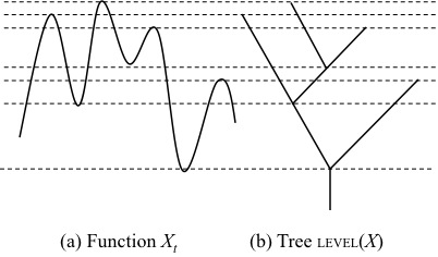
Figure 2. Function $X_{t}$ (panel a) with a finite number of local extrema and its level set tree $\textsc{level}(X)$ (panel b).

The level set tree $\textsc{level}(X_{t})$ is a planar time oriented binary tree that describes the topology of the level sets $\mathcal{L}_{\alpha}$ as a function of threshold $\alpha$, as illustrated in Fig. 2. Namely, there are bijections between (i) the leaves of $\textsc{level}(X_{t})$ and the local maxima of $X_{t}$, (ii) the internal (parental) vertices of $\textsc{level}(X_{t})$ and the local minima of $X_{t}$ (excluding possible local minima at the boundary points), and (iii) the pair of subtrees of $\textsc{level}(X_{t})$ rooted at a local minima $X(t^{*})$ and the first positive excursions (or meanders bounded by $t=0$ or $t=N$) of $X(t)-X(t^{*})$ to right and left of $t^{*}$. Each vertex in the tree is assigned a mark equal to the value of the local extrema according to the bijections (i) and (ii) above. This makes the tree time oriented according to the threshold $\alpha$. It is readily seen that any function $X_{t}$ with distinct values of consecutive local minima corresponds to a binary tree $\textsc{level}(X_{t})$. We refer to [22] for discussion of some subtleties related to this construction as well as for further references.

7.2. Tree representation of white noise

Let $W^{(N)}_{j}$, $j=1,\dots,N-1$, be a discrete white noise that is a discrete time process comprised of $N-1$ i.i.d. random variables with a common atomless distribution. Consider now an auxiliary process $\tilde{W}^{(N)}_{i}$, $i=1,\dots,2N-1$ such that it has exactly $N$ local maxima and $N-1$ internal local minima $\tilde{W}^{(N)}_{2j}=W^{(N)}_{j}$, $j=1,\dots,N-1$. We call $\tilde{W}^{(N)}_{i}$ an extended white noise; it can be constructed, for example, as follows:

(18) $$\tilde{W}^{(N)}_{i}=\left\{\begin{array}[]{cc}W^{(N)}_{i/2},&{\rm for~{}even~{}}i,\\ \max\left(W^{(N)}_{\max\left(1,\frac{i-1}{2}\right)},W^{(N)}_{\min\left(N-1,\frac{i+1}{2}\right)}\right)+1,&{\rm for~{}odd~{}}i.\end{array}\right.$$

Let $L^{(N)}_{W}=\textsc{level}\left(\tilde{W}^{(N)}_{i}\right)$ be the level set tree of $\tilde{W}^{(N)}_{i}$ and $\textsc{shape}\left(L^{(N)}_{W}\right)$ be a (random) combinatorial tree that retains the graph-theoretic structure of $L^{(N)}_{W}$ and drops its planar embedding as well as the vertex marks. By construction, $L^{(N)}_{W}$ has exactly $N$ leaves.

Lemma 9.

The distribution of $\textsc{shape}\left(L^{(N)}_{W}\right)$ on ${\mathcal{T}}_{N}$ is the same for any atomless distribution $F$ of the values of the associated white noise $W^{(N)}_{j}$.

Proof.

The condition of atomlessness of $F$ is necessary to ensure that the level set tree is binary with probability 1. By construction, the combinatorial level set tree is completely determined by the ordering of the local minima of the respective trajectory, independently of the particular values of its local maxima and minima. We complete the proof by noticing that the ordering of $W^{(N)}_{j}$ is the same for any choice of atomless distribution $F$. ∎

Let $T^{(N)}_{\rm K}$ be the tree that corresponds to a Kingman’s $N$-coalescent, and let $\textsc{shape}\left(T^{(N)}_{\rm K}\right)$ be its combinatorial version that drops the time marks of the vertices. Both the trees $\textsc{shape}\left(L^{(N)}_{W}\right)$ and $\textsc{shape}\left(T^{(N)}_{\rm K}\right)$, belong to the space ${\mathcal{T}}_{N}$ of binary rooted trees with $N$ leaves.

Theorem 2.

The trees $\textsc{shape}\left(L^{(N)}_{W}\right)$ and $\textsc{shape}\left(T^{(N)}_{\rm K}\right)$ have the same distribution on ${\mathcal{T}}_{N}$.

The proof below uses the duality between coalescence and fragmentation processes [1]. Recall that a fragmentation process starts with a single cluster of mass $N$ at time $t=0$. Each existing cluster of mass $m$ splits into two clusters of masses $m-x$ and $x$ at the splitting rate $S_{t}(m,x)$, $1<m\leq N$, $1\leq x<N$. A coalescence process on $N$ particles with time-dependent collision kernel $K_{t}(x,y)$, $1\leq x,y<N$ is equivalent, upon time reversal, to a discrete-mass fragmentation process of initial mass $N$ with some splitting kernel $S_{t}(m,x)$. See Aldous [1] for further details and the relationship between the dual collision and splitting kernels in general case.

Proof of Theorem 2.

We show that both the examined trees have the same distribution as the combinatorial tree of a fragmentation process with mass $N$ and a splitting kernel that is uniform in mass: $S_{t}(m,x)=S(t).$

Kingman’s $N$-coalescence with kernel $K(x,y)=1$ is dual to the fragmentation process with splitting kernel [1, Table 3]

$$S_{t}(m,x)=\frac{2}{t\,(t+2)}.$$

This kernel is independent of the cluster mass, which means that the splitting of mass $m$ is uniform among the $m-1$ possible pairs $\{1,m-1\}$, $~{}\{2,m-2\}$, $\ldots,\{m-1,1\}$. The time dependence of the kernel does not affect the combinatorial structure of the fragmentation tree (and can be removed by a deterministic time change.)

The level set tree $L^{(N)}_{W}$ can be viewed as a tree that describes a fragmentation process with the initial mass $N$ equal to the number of local maxima of the trajectory $\tilde{W}^{(N)}_{i}$. By construction, each subtree of $L^{(N)}_{W}$ with $n$ leaves corresponds to an excursion (or meander, if we treat one of the boundaries) with $n$ local maxima. This subtree (as well as the corresponding excursion or meander) splits into two by the internal global minimum of $\tilde{W}^{(N)}_{i}$ at the corresponding time interval.

The global minimum splits the series $\tilde{W}^{(N)}_{i}$ into two, to the left and right of the minimum, with $M_{L}$ and $(N-M_{L})$ local maxima, respectively. Since the local minima of $\tilde{W}^{(N)}_{i}$ form a white noise, the distribution of $M_{L}$ is uniform on $[1,N-1]$. Next, the internal vertices of the level set tree of the left (or right) time series correspond to its $M_{L}-1$ (or $N-M_{L}-1$) internal local minima that form a white noise (with the distribution different from that of the initial white noise $W^{(N)}_{j}$). Hence, the subsequent splits of masses (number of local maxima) continues according to a discrete uniform distribution. And so on down the tree.

Hence, the combinatorial level set tree of $\tilde{W}^{(N)}_{i}$ has the same distribution as a combinatorial tree of a fragmentation process with uniform mass splitting. This completes the proof. ∎

Remark 1.

We notice that the dual splitting kernels for multiplicative and additive coalescences [1, Table 3] only differ by their time dependence, and are equivalent as functions of mass. Hence, the combinatorial structure of the respective trees is the same.

Corollary 1.

The combinatorial level set tree of a discrete white noise $W^{(N)}$ is root-Horton self similar with the same Horton exponent $R$ as that for Kingman’s $N$-coalescent.

Proof.

Recall the operation of tree pruning ${\mathcal{R}}(T):{\mathcal{T}}\to{\mathcal{T}}$ that cuts the leaves of a finite tree $T$ and removes possible resulting nodes of degree 2 [4, 22]. By definition, pruning corresponds to index shift in Horton statistics: $N_{k}\to N_{k-1}$, $k>1$. It has been shown in [22] that

$${\mathcal{R}}\left[\textsc{level}\left(\tilde{W}^{(N)}_{i}\right)\right]=\textsc{level}\left(W^{(N)}_{j}\right).$$

Hence, Horton self-similarity for one of these processes implies that for the other. The Horton self-similarity for the extended white noise $\tilde{W}^{(N)}$ follows directly from Theorem 2. ∎

8. General coalescent processes

The ODE approach introduced in this paper can be extended to the coalescent kernels other than $K(i,j)\equiv 1$. For that we need to classify the relative number $\eta_{k}(t)$ of clusters of order $k$ at time $t$ according to the cluster masses. Namely, let $\eta_{k,m}(t)$ be the average number of clusters of order $k$ and mass $m\geq 2^{k}$ at time $t$. Then

$$\eta_{k}(t)=\sum\limits_{m=2^{k}}^{\infty}\eta_{k,m}(t).$$

In the case of a symmetric coalescent kernel $K(i,j)=K(j,i)$ the Smoluchowski-Horton ODEs can be written asymptotically as

$${d\over dt}\eta_{k,m}(t) = \sum\limits_{i=1}^{k-1}\sum\limits_{\mu=2^{k}}^{m-2^{i}}\eta_{k,\mu}(t)\eta_{i,m-\mu}K(\mu,m-\mu)$$

$$+ {1\over 2}\sum_{\begin{subarray}{c}m_{1}+m_{2}=m\\ m_{1},m_{2}\geq 2^{k-1}\end{subarray}}\eta_{k-1,m_{1}}(t)\eta_{k-1,m_{2}}(t)K(m_{1},m_{2})$$

$$- \eta_{k,m}(t)\sum\limits_{\widetilde{m}=2^{i}}^{\infty}K(m,\widetilde{m})\left(\sum\limits_{i=1}^{\infty}\eta_{i,\widetilde{m}}(t)\right)$$

with the initial conditions $\eta_{1,1}(0)=1~{}$ and $~{}\eta_{k,m}(0)=0$ for all $(k,m)\not=(1,1)$.

Observe that when $K(i,j)\equiv 1$, summing the above equations (8) over index $m$ produces the Smoluchowski-Horton ODE (2) for the average relative number of order-$k$ branches $\eta_{k}(t)$ in Kingman’s coalescent process.

9. Discussion

This paper establishes the root-Horton self-similarity (Sect. 6, Thm 1) for Kingman’s $N$-coalescent process, as $N$ goes to infinity. We also demonstrate (Sect. 7.1, Thm 2) the distributional equivalence of the combinatorial trees of Kingman’s $N$-coalescent to that of a discrete extended white noise with $N$ local maxima, hence extending the self-similarity results to a tree representation of a discrete white noise (Sect. 7, Cor 1).

Combining the results of this study with that of Burd et al. [4] and Zaliapin and Kovchegov [22] one observes that Horton self-similarity is a property of (i) white noise, (ii) symmetric random walk, (iii) critical binary Galton-Watson branching process, and (iv) Kingman’s $N$-coalescent. The listed processes are believed to closely depict physical and biological mechanisms of diverse origin and are commonly used as essential building blocks in scientific modeling. The results of this study and those in [4, 22] thus provide at least a partial explanation for the omnipresence of Horton self-similarity in observed and modeled branching structures. This study seems to be the first that rigorously establishes Horton self-similarity with Horton exponent different from $R=2,4$.

Our Theorem 1 establishes a weak, root-law, convergence of the asymptotic ratios ${\mathcal{N}}_{k}$, while we believe that the stronger (ratio and geometric) forms of convergence are also valid. These stronger Horton laws are usually considered in the literature (e.g., [14, 10, 7, 22]). It seems important to show rigorously at least the ratio-Horton law ($\lim\limits_{k\rightarrow\infty}{\mathcal{N}}_{k}/{\mathcal{N}}_{k+1}=R>0$).

The Smoluchowski-Horton equations (2) that form a core of the presented method and their equivalents (13) and (14) seem to be promising for further more detailed exploration. Indeed, one may hope that the approach that refers explicitly to the Horton-Strahler orders might effectively complement conventional analysis of cluster masses. The analysis of the Smoluchowski-Horton systems can be done within the ODE framework, similarly to the present study, or within the nonlinear iterative system framework (see (15)). The latter approach is still to be explored.

Finally, it is noteworthy that the analysis of multiplicative and additive coalescents according to the general Smoluchowski-Horton system (8) appears, after a certain series of transformations, to follow many of the steps implemented in this paper for Kingman’s coalescent, with the ODE system being replaced by a suitable PDE one. These results will be published elsewhere.

Acknowledgement. We are grateful to Ed Waymire for encouragement and continuing interest to this work. We thank the participants of the 2012 Oregon State University Workshop on Mathematical Problems in the Environmental Sciences for their constructive feedback. Suggestions of an anonymous reviewer and the Associate Editor helped to significantly improve the original manuscript.

Appendix A Proof of Lemma 1

Proof.

We split the proof into smaller steps.

$\bullet$ Step I. Fix $\epsilon_{0}\in(0,1)$ and take $\delta>0$. We show below that, given $\eta_{(N)}(t)=y\in{1\over N}\mathbb{Z}\cap[\epsilon_{0},1]$, the number of coalescences during the time interval $[t,t+\delta]$ does not exceed ${\delta\over N}\binom{N\,y}{2}+N^{2/3}$ with high probability. Specifically, we use exponential Markov inequality (aka Chernoff’s bound) with exponent $s>0$ to bound the probability that a sum of ${\delta\over N}\binom{N\,y}{2}+N^{2/3}$ exponential inter-arrival times with the rate not exceeding ${1\over N}\binom{N\,y}{2}$ adds up to less than $\delta$. Let $\zeta_{i}$ be the arrival time of $i$-th coalescence and $u=\binom{N\,y}{2}$. Then

$$\!\!\!\!\!\!\!\!\!\!\!\!\!\!\!\!\!\!\!\!\!\!\!\!\!\!\!\!\!\!\!\!\!\!\!\!\!\!\!\!\!\!\!\!P\left(N\big{[}\eta_{(N)}(t)-\eta_{(N)}(t+\delta)\big{]}>{\delta\over N}u+N^{2/3}~{}~{}\Big{|}~{}\eta_{(N)}(t)=y~{}\right)$$

$$= P\left(\sum_{i=1}^{\lfloor{\delta\over N}u+N^{2/3}\rfloor}\zeta_{i}<\delta~{}~{}\Big{|}~{}\eta_{(N)}(t)=y~{}\right)$$

$$\leq {e^{s\delta}\over\left(1+{s\,N\over u}\right)^{{\delta\over N}u+N^{2/3}}}$$

$$\leq \exp\left\{s\delta-\Big{(}{\delta\over N}u+N^{2/3}\Big{)}\left({s\,N\over u}-{s^{2}\,N^{2}\over u^{2}}\right)\right\}$$

$$= \exp\left\{-{s\over u}N^{5/3}+{\frac{\delta\,s^{2}}{u}\,N}+{s^{2}\over u^{2}}N^{8/3}\right\}$$

as $~{}\ln(1+x)>x-x^{2}~{}$ for $x>0$. Taking $s=N^{1/2}$ in the above inequality, we obtain

(20) $$\!\!\!\!\!\!\!\!\!\!\!\!\!\!\!\!\!\!\!\!\!\!\!\!\!\!\!\!\!\!\!\!\!\!\!\!\!\!\!\!\!\!\!\!P\left(N\big{[}\eta_{(N)}(t)-\eta_{(N)}(t+\delta)\big{]}>{\delta\over N}u+N^{2/3}~{}~{}\Big{|}~{}\eta_{(N)}(t)=y~{}\right)$$

$$= \exp\left\{-{1\over u}N^{13/6}+{\delta N^{2}\over u}+{N^{11/3}\over u^{2}}\right\}$$

$$= \exp\left\{-{2\over Ny(Ny-1)}N^{13/6}+{2\delta N^{2}\over Ny(Ny-1)}+{4N^{11/3}\over(Ny)^{2}(Ny-1)^{2}}\right\}$$

$$= \exp\left\{-{2\over y(y-1/N)}N^{1/6}+{2\delta\over y(y-1/N)}+{4N^{-1/3}\over(y)^{2}(y-1/N)^{2}}\right\}$$

$$\leq \exp\left\{-2N^{1/6}+{2\delta\over\epsilon_{0}(\epsilon_{0}-1/N)}+{4N^{-1/3}\over\epsilon_{0}^{2}(\epsilon_{0}-1/N)^{2}}\right\}$$

$$\leq \exp\left\{-N^{1/6}+{4\delta\over\epsilon_{0}^{2}}\right\}$$

for $N$ large enough.

$\bullet$ Step II. From Step I we know that, given $\eta_{(N)}(t)=y\in{1\over N}\mathbb{Z}\cap[\epsilon_{0},1]$, there are no more than

$${\delta\over N}\binom{Ny}{2}+N^{2/3}={\delta y^{2}\over 2}N-{\delta y\over 2}+N^{2/3}\leq{\delta y^{2}\over 2}N+N^{2/3}$$

coalescing pairs during $[t,t+\delta]$ with probability exceeding $1-\exp\left\{-N^{1/6}+{4\delta\over\epsilon_{0}^{2}}\right\}$. In this case the exponential rates of inter-arrival times during $[t,t+\delta]$ must be at least

$${1\over N}\binom{Ny-\lceil{\delta y^{2}\over 2}N\rceil-\lceil N^{2/3}\rceil}{2}={1\over N}\binom{Ny-\lceil{\delta y^{2}\over 2}N\rceil}{2}-{Ny-\lceil{\delta y^{2}\over 2}N\rceil-1/2-{\lceil N^{2/3}\rceil/2}\over N}\lceil N^{2/3}\rceil$$

$$\geq{1\over N}\binom{Ny-\lceil{\delta y^{2}\over 2}N\rceil}{2}-\left(y-{\delta y^{2}\over 2}\right)\lceil N^{2/3}\rceil\geq{1\over N}\binom{Ny-\lceil{\delta y^{2}\over 2}N\rceil}{2}-N^{2/3}$$

for $N$ large enough. We now use exponential Markov inequality to bound the conditional probability that there are fewer than ${\delta\over N}\binom{Ny-\lceil{\delta y^{2}\over 2}N\rceil}{2}-(1+\delta)N^{2/3}$ coalescents in $[t,t+\delta]$. Specifically, we bound the probability that a sum of ${\delta\over N}\binom{Ny-\lceil{\delta y^{2}\over 2}N\rceil}{2}-(1+\delta)N^{2/3}$ independent exponential random variables of rate not less than ${1\over N}\binom{Ny-\lceil{\delta y^{2}\over 2}N\rceil}{2}-N^{2/3}$ is greater than $\delta$.

Set $v=\binom{Ny-\lceil{\delta y^{2}\over 2}N\rceil}{2}$. Since we are interested in the values of $\delta\ll 1$, then

(21) $$(1-\delta)^{2}{N^{2}y^{2}\over 2}~{}\leq~{}v=\binom{Ny-\lceil{\delta y^{2}\over 2}N\rceil}{2}~{}\leq~{}u=\binom{Ny}{2}\leq{N^{2}y^{2}\over 2}.$$

Exponential Markov inequality with exponent $s>0$ implies

$P\left(N\big{[}\eta_{(N)}(t)-\eta_{(N)}(t+\delta)\big{]}<{\delta\over N}v-(1+\delta)N^{2/3}~{}~{}\Big{|}~{}\begin{array}[]{c}N\big{[}\eta_{(N)}(t)-\eta_{(N)}(t+\delta)\big{]}\leq{\delta\over N}u+N^{2/3}\\ \eta_{(N)}(t)=y\end{array}~{}\right)$

$$\leq {e^{-s\,\delta}\over\left(1-{s\,N\over v-N^{5/3}}\right)^{{\delta\over N}v-(1+\delta)N^{2/3}}}$$

$$\leq \exp\left\{-{s\,\delta}+\Big{(}{\delta\over N}v-(1+\delta)N^{2/3}\Big{)}\left({s\,N\over v-N^{5/3}}+{s^{2}\,N^{2}\over(v-N^{5/3})^{2}}\right)\right\}$$

$$\leq \exp\left\{\left({1\over 1-N^{5/3}/v}-1\right){s\,\delta}-{s(1+\delta)N^{5/3}\over v-N^{5/3}}+\Big{(}{\delta\over N}v-(1+\delta)N^{2/3}\Big{)}{s^{2}\,N^{2}\over(v-N^{5/3})^{2}}\right\}$$

$$\leq \exp\left\{{s\,\delta\,N^{5/3}/v\over 1-N^{5/3}/v}-{s(1+\delta)N^{5/3}\over v}+{\delta\,v\,s^{2}\,N\over(v-N^{5/3})^{2}}\right\}$$

as $~{}-x-x^{2}<\ln(1-x)$ for $x\in\left(0,{1\over 2}\right)$. Take $s=N^{1/2}$ to obtain

$P\left(N\big{[}\eta_{(N)}(t)-\eta_{(N)}(t+\delta)\big{]}<{\delta\over N}v-(1+\delta)N^{2/3}~{}~{}\Big{|}~{}\begin{array}[]{c}N\big{[}\eta_{(N)}(t)-\eta_{(N)}(t+\delta)\big{]}\leq{\delta\over N}u+N^{2/3}\\ \eta_{(N)}(t)=y\end{array}~{}\right)$

(22) $$= \exp\left\{{\delta N^{13/6}/v\over 1-N^{5/3}/v}-{(1+\delta)N^{13/6}\over v}+{\delta vN^{2}\over(v-N^{5/3})^{2}}\right\}$$

$$\leq \exp\left\{{2\delta N^{1/6}\over(1-\delta)^{2}y^{2}-2N^{-1/3}}-{2(1+\delta)N^{1/6}\over y^{2}}+{2\delta y^{2}\over\left((1-\delta)^{2}y^{2}-2N^{-1/3}\right)^{2}}\right\}$$

$$\leq \exp\left\{{2N^{1/6}\over y^{2}}\left[{\delta\over(1-\delta)^{2}-2N^{-1/3}/y^{2}}-(1+\delta)\right]+{3\delta y^{2}\over(1-\delta)^{4}y^{4}}\right\}$$

$$\leq \exp\left\{-{N^{1/6}\over y^{2}}+{3\delta\over(1-\delta)^{4}y^{2}}\right\}$$

$$\leq \exp\left\{-N^{1/6}+{4\delta\over\epsilon_{0}^{2}}\right\}$$

for $N$ large enough, by using (21).

Thus, multiplying the probabilities of complement events in (20) and (22) we obtain

$P\left({\delta\over N^{2}}v-(1+\delta)N^{-1/3}\leq\eta_{(N)}(t)-\eta_{(N)}(t+\delta)\leq{\delta\over N^{2}}u+N^{-1/3}~{}~{}\Big{|}~{}\eta_{(N)}(t)=y~{}\right)$

$$\geq\left(1-\exp\left\{-N^{1/6}+{4\delta\over\epsilon_{0}^{2}}\right\}\right)^{2}$$

for any given $t\geq 0$ and $y\in{1\over N}\mathbb{Z}\cap[\epsilon_{0},1]$.

$\bullet$ Step III. Now, as we already pointed out in (21),

$$~{}(1-\delta)^{2}{N^{2}\eta^{2}_{(N)}(t)\over 2}~{}\leq~{}v~{}\leq~{}u~{}\leq~{}{N^{2}\eta^{2}_{(N)}(t)\over 2}.$$

Hence,

$P\left(~{}\left|{\eta^{2}_{(N)}(t)\over 2}+\Delta_{\delta}\eta_{(N)}(t)\right|~{}\leq~{}\delta+(\delta^{-1}+1)N^{-1/3}~{}~{}\Big{|}~{}\eta_{(N)}(t)=y~{}\right)$
$\geq P\left((1-\delta)^{2}{\eta^{2}_{(N)}(t)\over 2}-(\delta^{-1}+1)N^{-1/3}\leq-\Delta_{\delta}\eta_{(N)}(t)\leq{\eta^{2}_{(N)}(t)\over 2}+\delta^{-1}N^{-1/3}~{}~{}\Big{|}~{}\eta_{(N)}(t)=y~{}\right)$
$\geq P\left({\delta\over N^{2}}v-(1+\delta)N^{-1/3}\leq\eta_{(N)}(t)-\eta_{(N)}(t+\delta)\leq{\delta\over N^{2}}u+N^{-1/3}~{}~{}\Big{|}~{}\eta_{(N)}(t)=y~{}\right)$

(23) $$\geq\left(1-\exp\left\{-N^{1/6}+{4\delta\over\epsilon_{0}^{2}}\right\}\right)^{2}$$

for $N$ large enough, where $~{}\Delta_{\delta}f(x):={f(x+\delta)-f(x)\over\delta}~{}$ denotes the forward difference. The first inequality above uses the fact that

$$(1-\delta)^{2}\,\frac{\eta_{(N)}^{2}(t)}{2}>\frac{\eta_{(N)}^{2}(t)}{2}-\delta.$$

This is equivalent to

$$(-2+\delta)\,\frac{\eta_{(N)}^{2}(t)}{2}>-1,$$

which is always true since $\eta_{(N)}(t)\leq 1$ and $\delta>0$.

$\bullet$ Step IV. For $K>0$, consider an interval $[0,K]$ partitioned into $M$ subintervals

$$[t_{0},t_{1}],~{}[t_{1},t_{2}],~{}\ldots,~{}[t_{M-1},t_{M}]$$

of equal length $\delta=K/M$, where $t_{0}=0$ and $t_{M}=K$.

Let $\epsilon_{0}=\eta(K)/2=1/(2+K)$, where $\eta(t)=2/(2+t)$ is the solution to the equation (1) with the initial condition $\eta(0)=1$. Consider the following difference equation

(24) $$\Delta_{\delta}\psi_{(N)}(t_{i})=-{\psi_{(N)}^{2}(t_{i})\over 2}+\mathcal{E}^{\prime}(t_{i})$$

with initial condition $\psi_{(N)}(0)=1$, where the error $~{}|\mathcal{E}^{\prime}(t_{i})|\leq\delta+(\delta^{-1}+1)N^{-1/3}$.

Claim 1. If $M$ is large enough, then the following is true as we take $N$ large enough. For any natural number $j\leq M$, if function $\psi_{(N)}(t_{i})$ satisfies (24) for all $i\in\{0,1,\ldots,j-1\}$, then

$$\psi_{(N)}(t_{j})\geq\epsilon_{0}.$$

Indeed, if we take $N\geq M^{6}$, then

$$|\mathcal{E}^{\prime}(t_{i})|\leq\delta+(\delta^{-1}+1)N^{-1/3}\leq K/M+1/(KM)+1/M^{2}.$$

Now, since $\eta(t)=2/(2+t)$ is the solution to the equation (1) with the initial condition $\eta(0)=1$, $\eta(t)$ will satisfy

$$\Delta_{\delta}\eta(t_{i})=-{\eta^{2}(t_{i})\over 2}+\mathcal{E}(t_{i})$$

for all $i\in\{0,1,\ldots,M-1\}$, where $~{}\mathcal{E}(t_{i})={\eta^{\prime\prime}(c_{i})\over 2}\delta={\eta^{3}(c_{i})\over 4}\delta$ for some $c_{i}\in(t_{i},t_{i+1})$. Hence, as $\eta(t)\leq 1$ for all $t\geq 0$, $~{}|\mathcal{E}(t_{i})|\leq{1\over 4}\delta$.

Consider the error quantities $~{}\varepsilon_{i}:=\psi_{(N)}(t_{i})-\eta(t_{i})$. We have

$$\varepsilon_{i+1} = \psi_{(N)}(t_{i+1})-\eta(t_{i+1})$$

$$= \left[\psi_{(N)}(t_{i})-{\psi^{2}_{(N)}(t_{i})\over 2}\delta+\mathcal{E}^{\prime}(t_{i})\delta\right]-\left[\eta(t_{i})-{\eta^{2}(t_{i})\over 2}\delta+\mathcal{E}(t_{i})\delta\right]$$

$$= \left[\eta(t_{i})+\varepsilon_{i}-{\Big{(}\eta(t_{i})+\varepsilon_{i}\Big{)}^{2}\over 2}\delta+\mathcal{E}^{\prime}(t_{i})\delta\right]-\left[\eta(t_{i})-{\eta^{2}(t_{i})\over 2}\delta+\mathcal{E}(t_{i})\delta\right]$$

$$= (1-\eta(t_{i})\delta)\varepsilon_{i}-{\varepsilon_{i}^{2}\over 2}\delta+\delta\Big{(}\mathcal{E}^{\prime}(t_{i})-\mathcal{E}(t_{i})\Big{)},$$

where $~{}\Big{|}\mathcal{E}^{\prime}(t_{i})-\mathcal{E}(t_{i})\Big{|}\leq{5\over 4}K/M+1/(KM)+1/M^{2}<C_{K}/M~{}$ if $M>1$, with $C_{K}={5\over 4}K+\frac{1}{K}+1$. Since $\eta(t_{i})>\eta(K)$ for all $i\in\{0,1,\ldots,M-1\}$,

$$|\varepsilon_{i+1}|\leq(1-\eta(K)K/M)|\varepsilon_{i}|+{\varepsilon_{i}^{2}\over 2}K/M+KC_{K}/M^{2}.$$

Taking $M$ large enough so that $KC_{K}/M<2\eta(K)$, we can prove by induction that

(25) $$|\varepsilon_{i}|\leq iKC_{K}/M^{2}.$$

Indeed, $\varepsilon_{0}=0$, and if $|\varepsilon_{i}|\leq iKC_{K}/M^{2}$, then

$$|\varepsilon_{i+1}| \leq (1-\eta(K)K/M)|\varepsilon_{i}|+{\varepsilon_{i}^{2}\over 2}K/M+KC_{K}/M^{2}$$

$$= |\varepsilon_{i}|+\big{(}|\varepsilon_{i}|-2\eta(K)\big{)}|\varepsilon_{i}|K/(2M)+KC_{K}/M^{2}$$

$$\leq |\varepsilon_{i}|+\big{(}iKC_{K}/M^{2}-2\eta(K)\big{)}|\varepsilon_{i}|K/(2M)+KC_{K}/M^{2}$$

$$\leq |\varepsilon_{i}|+KC_{K}/M^{2}$$

$$\leq (i+1)KC_{K}/M^{2},$$

which completes the induction step.
The inequality (25) is therefore valid for all $i\in\{0,\ldots,M-1\}$, implying

(26) $$|\varepsilon_{i}|\leq MKC_{K}/M^{2}=\frac{{5\over 4}K^{2}+K+1}{M}<\epsilon_{0}$$

for $M$ large enough.

Recall that $\epsilon_{0}=\eta(K)/2=1/(2+K)$. Then, by (26),

$$\psi_{(N)}(t_{j})=\eta(t_{j})+\varepsilon_{j}\geq\eta(K)-\epsilon_{0}=\epsilon_{0}$$

for all $j\in\{0,1,\ldots,M-1\}$. This proves the above Claim 1.

$\bullet$ Step V. Consider events

(27) $$A_{i}=\left\{~{}\Delta_{\delta}\eta_{(N)}(t_{i})=-{\eta^{2}_{(N)}(t_{i})\over 2}+\mathcal{E}^{\prime}(t_{i})~{}\text{ and }~{}|\mathcal{E}^{\prime}(t_{i})|~{}\leq\delta+(\delta^{-1}+1)N^{-1/3}~{}\right\}$$

for all $i\in\{0,1,\ldots,M-1\}$. Then inequality (23) rewrites as

$$P\left(~{}A_{j}~{}\Big{|}~{}\eta_{(N)}(t_{j})=y~{}\right)\geq\left(1-\exp\left\{-N^{1/6}+{4\delta\over\epsilon_{0}^{2}}\right\}\right)^{2}$$

for any $y\in{1\over N}\mathbb{Z}\cap[\epsilon_{0},1]$.

Claim 1 implies that $\bigcap\limits_{i=0}^{j-1}A_{i}$ is contained in the event $\{~{}\eta_{(N)}(t_{j})\in[\epsilon_{0},1]~{}\}$, and therefore

$$P\left(~{}A_{j}~{}\Big{|}~{}\bigcap\limits_{i=0}^{j-1}A_{i}~{}\right) = \sum\limits_{y:~{}y\in{1\over N}\mathbb{Z}\cap[\epsilon_{0},1]}P\left(~{}A_{j}~{}\Big{|}~{}\eta_{(N)}(t_{j})=y,~{}\bigcap\limits_{i=0}^{j-1}A_{i}~{}\right)P\left(\eta_{(N)}(t_{j})=y~{}\Big{|}~{}\bigcap\limits_{i=0}^{j-1}A_{i}~{}\right)$$

$$= \sum\limits_{y:~{}y\in{1\over N}\mathbb{Z}\cap[\epsilon_{0},1]}P\left(~{}A_{j}~{}\Big{|}~{}\eta_{(N)}(t_{j})=y~{}\right)P\left(\eta_{(N)}(t_{j})=y~{}\Big{|}~{}\bigcap\limits_{i=0}^{j-1}A_{i}~{}\right)$$

$$\geq \left(1-\exp\left\{-N^{1/6}+{4\delta\over\epsilon_{0}^{2}}\right\}\right)^{2}.$$

as $\sum\limits_{y:~{}y\in{1\over N}\mathbb{Z}\cap[\epsilon_{0},1]}P\left(\eta_{(N)}(t_{j})=y~{}\Big{|}~{}\bigcap\limits_{i=0}^{j-1}A_{i}~{}\right)=P\left(\eta_{(N)}(t_{j})\in[\epsilon_{0},1]~{}\Big{|}~{}\bigcap\limits_{i=0}^{j-1}A_{i}~{}\right)=1$. Hence, since we have taken $N\geq M^{6}$,

$$P\left(~{}\bigcap\limits_{i=0}^{M-1}A_{i}~{}\right) \geq \left(1-\exp\left\{-N^{1/6}+{4\delta\over\epsilon_{0}^{2}}\right\}\right)^{2M}$$

$$\geq \left(1-\exp\left\{-M+{4K\over\epsilon_{0}^{2}M}\right\}\right)^{2M}$$

$$\rightarrow 1\quad\text{ as }M\rightarrow\infty.$$

We established that with probability greater than $P\left(~{}\bigcap\limits_{i=0}^{M-1}A_{i}~{}\right)\rightarrow 1$ as $M\rightarrow\infty$, $\eta_{(N)}(t_{i})$ satisfies difference equation (24) with $\psi_{(N)}(t)\equiv\eta_{(N)}(t)$.

$\bullet$ Step VI. Rewriting (26) for $\psi_{(N)}(t)\equiv\eta_{(N)}(t)$, we see that with probability of at least $P\left(~{}\bigcap\limits_{i=0}^{M-1}A_{i}~{}\right)\rightarrow 1$,

$$\big{|}\eta_{(N)}(t_{i})-\eta(t_{i})\big{|}~{}=|\varepsilon_{i}|~{}<\epsilon_{0}$$

for all $i\in\{0,1,\ldots,M-1\}$. Now, if $t\in(t_{i},t_{i+1})$, then

$$\big{|}\eta_{(N)}(t)-\eta(t)\big{|} \leq \big{|}\eta_{(N)}(t)-\eta_{(N)}(t_{i})\big{|}+\big{|}\eta_{(N)}(t_{i})-\eta(t_{i})\big{|}+\big{|}\eta(t_{i})-\eta(t)\big{|}$$

$$\leq \big{(}\eta_{(N)}(t_{i})-\eta_{(N)}(t_{i+1})\big{)}+\left({5\over 4}K^{2}+K+1\right)/M+\big{(}\eta(t_{i})-\eta(t_{i+1})\big{)}$$

$$= \eta_{(N)}(t_{i})-\eta(t_{i})+\eta(t_{i+1})-\eta_{(N)}(t_{i+1})+\left({5\over 4}K^{2}+K+1\right)/M+2\big{(}\eta(t_{i})-\eta(t_{i+1})\big{)}$$

$$\leq 3\left({5\over 4}K^{2}+K+1\right)/M+2\big{(}\eta(t_{i})-\eta(t_{i+1})\big{)}$$

$$\leq 3\left({5\over 4}K^{2}+K+1\right)/M+\delta.$$

as

(29) $$2\big{(}\eta(t_{i})-\eta(t_{i+1})\big{)}=2\delta{d\over dt}\eta(c_{i})=\delta\,\eta^{2}(c_{i})\leq\delta~{}~{}\text{ for some }c_{i}\in[t_{i},t_{i+1}].$$

Here we used the facts that $\eta_{(N)}(t)$ and $\eta(t)$ are decreasing functions and $\eta(t)=2/(2+t)$ is the solution to Eq. (1). Thus with probability greater than $P\left(~{}\bigcap\limits_{i=0}^{M-1}A_{i}~{}\right)\rightarrow 1$,

(30) $$\big{\|}\eta_{(N)}(t)-\eta(t)\big{\|}_{L^{\infty}[0,K]}\leq\left({15\over 4}K^{2}+3K+3\right)/M+K/M={15\over 4}K^{2}/M+4K/M+3/M$$

for $M$ large enough and $N\geq M^{6}$.

Therefore, letting $M\rightarrow\infty$, we have shown that

$$\big{\|}\eta_{(N)}(t)-\eta(t)\big{\|}_{L^{\infty}[0,K]}\rightarrow 0\qquad\text{ in probability.}$$

$\bullet$ Step VII. Take $\epsilon\in(0,1)$ and $\gamma>1$. Let $T_{m}$ be the time when the first $m=\lfloor(1-\epsilon)N\rfloor$ clusters merge. The expectation for the time $T_{m}$ is

$$E[T_{m}]={N\over\binom{N}{2}}+{N\over\binom{N-1}{2}}+\dots+{N\over\binom{N-m+1}{2}}={2m\over N-m}.$$

If we take $K>{2(1-\epsilon)\over\epsilon}\gamma$, then $\eta(K)<\eta\left({2(1-\epsilon)\over\epsilon}\gamma\right)<\eta\big{(}2(1-\epsilon)/\epsilon\big{)}=\epsilon$, and for any $t\geq K$, $~{}\big{|}\eta_{(N)}(t)-\eta(t)\big{|}>\epsilon~{}$ implies $~{}\eta_{(N)}(t)>\epsilon>\eta(t)>0$. Thus, by Markov’s inequality,

(31) $$P\Big{(}\big{\|}\eta_{(N)}(t)-\eta(t)\big{\|}_{L^{\infty}[K,\infty)}>\epsilon\Big{)} \leq P\Big{(}\eta_{(N)}(K)>\epsilon\Big{)}=P\Big{(}T_{m}>K\Big{)}$$

$$\leq {2(1-\epsilon)\over\epsilon K}<1/\gamma.$$

Now, we take $M>\left({15\over 4}K^{2}+4K+3\right)/\epsilon$. Then, by (30),

$$P\Big{(}\big{\|}\eta_{(N)}(t)-\eta(t)\big{\|}_{L^{\infty}[0,K]}<\epsilon\Big{)}\geq P\left(~{}\bigcap\limits_{i=0}^{M-1}A_{i}~{}\right),$$

and

$$P\Big{(}\big{\|}\eta_{(N)}(t)-\eta(t)\big{\|}_{L^{\infty}[0,\infty)}<\epsilon\Big{)} \geq P\Big{(}\big{\|}\eta_{(N)}(t)-\eta(t)\big{\|}_{L^{\infty}[0,K]}<\epsilon\Big{)}$$

$$\qquad+P\Big{(}\big{\|}\eta_{(N)}(t)-\eta(t)\big{\|}_{L^{\infty}[K,\infty)}<\epsilon\Big{)}-1$$

$$\geq P\left(~{}\bigcap\limits_{i=0}^{M-1}A_{i}~{}\right)+(1-1/\gamma)-1$$

$$\rightarrow 1-1/\gamma$$

as we let $~{}M\rightarrow\infty$. Hence,

$$\limsup\limits_{N\rightarrow\infty}P\Big{(}\big{\|}\eta_{(N)}(t)-\eta(t)\big{\|}_{L^{\infty}[0,\infty)}<\epsilon\Big{)}\geq 1-1/\gamma$$

for any given $\gamma>1$. Thus

$$\lim\limits_{N\rightarrow\infty}P\Big{(}\big{\|}\eta_{(N)}(t)-\eta(t)\big{\|}_{L^{\infty}[0,\infty)}<\epsilon\Big{)}=1.$$

Therefore we have shown that $~{}\|\eta_{(N)}(t)-\eta(t)\|_{L^{\infty}[0,\infty)}\rightarrow 0~{}$ in probability. ∎

Appendix B Proof of Lemma 2

Proof.

$\bullet$ Step I. We will use the setting from the proof of Lemma 1. Fix $K>0$ and consider an interval $[0,K]$ partitioned into $M$ subintervals

$$[t_{0},t_{1}],~{}[t_{1},t_{2}],~{}\ldots,~{}[t_{M-1},t_{M}]$$

of equal length $\delta=K/M$, where $t_{0}=0$ and $t_{M}=K$. Let $\epsilon_{0}=\eta(K)/2=1/(2+K)$.

Once again, let $\eta_{(N)}(t)$ denote the relative total number of clusters. For $i=0,1,\ldots,M-1$, the total number of coalescences within the interval $[t_{i},t_{i+1}]$ equals $N\big{[}\eta_{(N)}(t_{i})-\eta_{(N)}(t_{i+1})\big{]}$. Take $N>M^{6}$. The probability of the event $~{}\bigcap\limits_{i=0}^{M-1}A_{i}$, where $A_{i}$ was defined in (27), was bounded below in (A) as follows
$P\left(\left|N\big{[}\eta_{(N)}(t_{i})-\eta_{(N)}(t_{i+1})\big{]}-\delta N{\eta^{2}_{(N)}(t_{i})\over 2}\right|~{}\leq\delta^{2}N+(1+\delta)N^{2/3}\qquad\forall i=0,1,\ldots,M-1\right)$

$$=P\Big{(}\bigcap\limits_{i=0}^{M-1}A_{i}~{}\Big{)}~{}\geq~{}\left(1-\exp\left\{-M+{4K\over\epsilon_{0}^{2}M}\right\}\right)^{2M}\rightarrow 1$$

as $~{}M\rightarrow\infty$. Recall also that $~{}P\Big{(}\min\limits_{t\in[0,K]}\eta_{(N)}(t)>\epsilon_{0}~{}\Big{|}~{}\bigcap\limits_{i=0}^{M-1}A_{i}~{}\Big{)}=1$.

Recall $\eta_{k,N}(t)$ is the number of clusters corresponding to branches of Horton-Strahler order $k$ at time $t$ relative to the system size $N$, and let $~{}g_{k,N}(t):=\eta_{(N)}(t)-\sum\limits_{j:~{}j<k}\eta_{j,N}(t)$. For any $m_{i}>0$ consider a conditional probability measure $P_{i,m_{i}}$ where we condition on $~{}\bigcap\limits_{i^{\prime}=0}^{i-1}A_{i^{\prime}}~{}$ and the values of functions $\{\eta_{j,N}(t_{i})\}_{j=0,1,\ldots}$ such that $~{}\eta_{(N)}(t_{i})=\sum\limits_{j=0}^{\infty}\eta_{j,N}(t_{i})~{}$ satisfies

(32) $$\left|m_{i}-\delta N{\eta^{2}_{(N)}(t_{i})\over 2}\right|~{}\leq\delta^{2}N+(1+\delta)N^{2/3}.$$

Let $E_{i,m_{i}}$ denote the corresponding conditional expectation. Consider the following events:

$$B_{m_{i},t_{i}}=\Big{\{}\text{ inequality (\ref{ineq:mi}) is satisfied}\Big{\}},$$

$$D_{m_{i},t_{i}}=\Big{\{}N\big{[}\eta_{(N)}(t_{i})-\eta_{(N)}(t_{i+1})\big{]}=m_{i}\Big{\}}.$$

We observe that

(33) $$A_{i}=\bigcup\limits_{m_{i}}\Big{[}B_{m_{i},t_{i}}\cap D_{m_{i},t_{i}}\Big{]},$$

so $P_{i,m_{i}}$ is a conditional probability, where we condition on a subevent of $\bigcap\limits_{i^{\prime}=0}^{i}A_{i^{\prime}}$.

For any $k\in\mathbb{N}^{+}$ we can represent the coalescences that involve the clusters of order $k$ within $[t_{i},t_{i+1}]$ as

$$\eta_{k,N}(t_{i+1})-\eta_{k,N}(t_{i})=\xi_{1}+\xi_{2}+\ldots+\xi_{m_{i}},$$

where $~{}\xi_{1},\xi_{2},\ldots,\xi_{m_{i}}~{}$ are random variables that correspond to the $m_{i}$ coalescences (of any Horton-Strahler order) within $[t_{i},t_{i+1}]$ in the order of occurrence. Here, each $\xi_{r}$ can take values in $\frac{1}{N}\{-2,-1,0,1\}$; and their dependence on $k$ is omitted to simplify the notations. By construction, the distribution of $\xi_{r}$ for $1\leq r\leq m_{i}$ is completely determined by the history $~{}\mathcal{T}_{r-1}$ of the preceding $r-1$ transitions. Specifically,

1. A transition that decreases $\eta_{k,N}(t)$ by $2/N$ has probability

   $$p_{l}(-2)~{}\leq P_{i,m_{i}}\left(\xi_{r}=-2/N~{}\Big{|}~{}D_{m_{i},t_{i}},~{}\mathcal{T}_{r-1}\right)\leq p_{u}(-2),$$

   where

   $$p_{l}(-2):=\begin{cases}{\binom{N\eta_{k,N}(t_{i})-2\,m_{i}}{2}/\binom{N\eta_{(N)}(t_{i})}{2}}&\text{ if }N\eta_{k,N}(t_{i})-2\,m_{i}\geq 2\\ 0&\text{ otherwise }\end{cases},$$

   and $~{}p_{u}(-2):={\binom{N\eta_{k,N}(t_{i})}{2}/\binom{N\eta_{(N)}(t_{i})-m_{i}}{2}}$.
   

2. A transition that increases $\eta_{k,N}(t)$ by $1/N$ has probability

   $$p_{l}(1)~{}\leq P_{i,m_{i}}\left(\xi_{r}=1/N~{}\Big{|}~{}D_{m_{i},t_{i}},~{}\mathcal{T}_{r-1}\right)\leq p_{u}(1),$$

   where

   $$p_{l}(1):=\begin{cases}{\binom{N\eta_{k-1,N}(t_{i})-2\,m_{i}}{2}/\binom{N\eta_{(N)}(t_{i})}{2}}&\text{ if }N\eta_{k-1,N}(t_{i})-2\,m_{i}\geq 2\\ 0&\text{ otherwise }\end{cases},$$

   and $~{}p_{u}(1):={\binom{N\eta_{k-1,N}(t_{i})}{2}/\binom{N\eta_{(N)}(t_{i})-m_{i}}{2}}$ if $k>1$, and if $k=1$, we let $p_{l}(1)=p_{u}(1)=0$.
   

3. A transition that decreases $\eta_{k,N}(t)$ by $1/N$ has probability

   $$p_{l}(-1)~{}\leq P_{i,m_{i}}\left(\xi_{r}=-1/N~{}\Big{|}~{}D_{m_{i},t_{i}},~{}\mathcal{T}_{r-1}\right)~{}\leq p_{u}(-1)$$

   where $~{}p_{l}(-1):={\max\{(N\eta_{k,N}(t_{i})-2\,m_{i}),0\}Ng_{k+1,N}(t_{i})/\binom{N\eta_{(N)}(t_{i})}{2}}~{}$ and
   
   $p_{u}(-1):={N^{2}\eta_{k,N}(t_{i})g_{k+1,N}(t_{i})/\binom{N\eta_{(N)}(t_{i})-m_{i}}{2}}$.

Next, let $~{}p(-2):=\eta^{2}_{k,N}(t_{i})/\eta^{2}_{(N)}(t_{i})$,   $p(1):=\begin{cases}\eta^{2}_{k-1,N}(t_{i})/\eta^{2}_{(N)}(t_{i})&\text{ if }k>1\\ 0&\text{ if }k=1\end{cases}$,

$p(-1):=2\eta_{k,N}(t_{i})g_{k+1,N}(t_{i})/\eta^{2}_{(N)}(t_{i})$,  $~{}p(0):=1-p(-2)-p(-1)-p(1)$, and $\xi$ be a random variable with the values $\{-2,-1,0,1\}$ specified by the probabilities $\{p(-2),p(-1),p(0),p(1)\}$. Also let $~{}\xi^{+}=\xi\cdot{\bf 1}_{\xi>0}~{}$ and $~{}\xi^{-}=\xi\cdot{\bf 1}_{\xi<0}$.

Observe that since we conditioned on a sub-event of $\bigcap\limits_{i^{\prime}=0}^{i}A_{i^{\prime}}$, then $\eta_{(N)}(t_{i})\geq\epsilon_{0}$ and therefore

$$p_{l}(-2)=p(-2)+\mathcal{O}(\delta)\quad\text{ and }\quad p_{u}(-2)=p(-2)+\mathcal{O}(\delta),$$

$$p_{l}(1)=p(1)+\mathcal{O}(\delta)\quad\text{ and }\quad p_{u}(1)=p(1)+\mathcal{O}(\delta),$$

$$p_{l}(-1)=p(-1)+\mathcal{O}(\delta)\quad\text{ and }\quad p_{u}(-1)=p(-1)+\mathcal{O}(\delta).$$

Let $~{}\xi_{r}^{+}=\xi_{r}\cdot{\bf 1}_{\xi_{r}>0}~{}$ and $~{}\xi_{r}^{-}=\xi_{r}\cdot{\bf 1}_{\xi_{r}<0}$. Then

$$\eta_{k,N}(t_{i+1})-\eta_{k,N}(t_{i})=X_{+}+X_{-},$$

where

$$X_{+}=\xi_{1}^{+}+\xi_{2}^{+}+\ldots+\xi_{m_{i}}^{+}$$

and

$$X_{-}=\xi_{1}^{-}+\xi_{2}^{-}+\ldots+\xi_{m_{i}}^{-}.$$

Next, for any $\lambda^{+},\lambda^{-}\geq 0$ and $s\in[0,1]$ consider

$$E_{i,m_{i}}\left[e^{sN\big{[}\lambda^{+}X_{+}+\lambda^{-}X_{-}\big{]}}~{}\Big{|}~{}D_{m_{i},t_{i}}\right]=\prod\limits_{r=1}^{m_{i}}E_{i,m_{i}}\left[e^{sN[\lambda^{+}\xi_{r}^{+}+\lambda^{-}\xi_{r}^{-}]}~{}\Big{|}~{}D_{m_{i},t_{i}},\mathcal{T}_{r-1}\right],$$

where for all $r$,

$$E_{i,m_{i}}\left[e^{sN[\lambda^{+}\xi_{r}^{+}+\lambda^{-}\xi_{r}^{-}]}~{}\Big{|}~{}D_{m_{i},t_{i}},\mathcal{T}_{r-1}\right]$$

$$\leq e^{-2\lambda^{-}s}p_{u}(-2)+e^{-\lambda^{-}s}p_{u}(-1)+e^{\lambda^{+}s}p_{u}(1)+(1-p_{l}(-2)-p_{l}(-1)-p_{l}(1))$$

$$\leq e^{-2\lambda^{-}s}p(-2)+e^{-\lambda^{-}s}p(-1)+e^{\lambda^{+}s}p(1)+p(0)+C\delta$$

$$= E\left[e^{s\,[\lambda^{+}\xi^{+}+\lambda^{-}\xi^{-}]}\right]+C\delta$$

for large enough $C>0$. Hence,

$$E_{i,m_{i}}\left[e^{sN\big{[}\lambda^{+}X_{+}+\lambda^{-}X_{-}\big{]}}~{}\Big{|}~{}D_{m_{i},t_{i}}\right]\leq\Big{(}E\left[e^{s\,[\lambda^{+}\xi^{+}+\lambda^{-}\xi^{-}]}\right]+C\delta\Big{)}^{m_{i}}.$$

Therefore, by the exponential Markov inequality with the exponent $s$, for any $m_{i}$ such that (32) is satisfied,

$$P_{i,m_{i}}\Big{(}N\big{[}\lambda^{+}X_{+}+\lambda^{-}X_{-}\big{]}\geq E[\lambda^{+}\xi^{+}+\lambda^{-}\xi^{-}]\,m_{i}+m_{i}^{14/15}~{}\Big{|}~{}D_{m_{i},t_{i}}~{}\Big{)}$$

$$~{}~{}~{}\leq E_{i,m_{i}}\left[e^{sN\big{[}\lambda^{+}X_{+}+\lambda^{-}X_{-}\big{]}}~{}\Big{|}~{}D_{m_{i},t_{i}}\right]e^{-s\big{(}E[\lambda^{+}\xi^{+}+\lambda^{-}\xi^{-}]\,m_{i}+m_{i}^{14/15}\big{)}}$$

$$~{}~{}~{}\leq \Big{(}E\left[e^{s\,[\lambda^{+}\xi^{+}+\lambda^{-}\xi^{-}]}\right]+C\delta\Big{)}^{m_{i}}e^{-s\big{(}E[\lambda^{+}\xi^{+}+\lambda^{-}\xi^{-}]\,m_{i}+m_{i}^{14/15}\big{)}}$$

$$~{}~{}~{}= \Big{(}E\left[e^{s(\lambda^{+}[\xi^{+}-E[\xi^{+}]]+\lambda^{-}[\xi^{-}-E[\xi^{-}]])}\right]+e^{-sE[\lambda^{+}\xi^{+}+\lambda^{-}\xi^{-}]}C\delta\Big{)}^{m_{i}}e^{-sm_{i}^{14/15}}$$

$$~{}~{}~{}= \Big{(}1+E\left[s\left(\lambda^{+}[\xi^{+}-E[\xi^{+}]]+\lambda^{-}[\xi^{-}-E[\xi^{-}]]\right)\right]+C\delta+\mathcal{O}(s^{2}+s\delta)\Big{)}^{m_{i}}e^{-sm_{i}^{14/15}}$$

$$~{}~{}~{}= \Big{(}1+C\delta+\mathcal{O}(s^{2}+s\delta)\Big{)}^{m_{i}}e^{-sm_{i}^{14/15}}$$

$$~{}~{}~{}\leq \exp\left\{m_{i}\big{[}C\delta+\mathcal{O}(s^{2}+s\delta)\big{]}-sm_{i}^{14/15}\right\},\quad{\rm as~{}}s,\delta\to 0.$$

Next, taking $2M^{6}>N>M^{6}$ and $M$ large enough, and plugging $s=2C\delta m_{i}^{1/15}=\mathcal{O}(M^{-2/3})$ (as $M\rightarrow\infty$) into the above exponential Markov inequality, we obtain

(34) $$P_{i,m_{i}}\Big{(}N\big{[}\lambda^{+}X_{+}+\lambda^{-}X_{-}\big{]}\geq E[\lambda^{+}\xi^{+}+\lambda^{-}\xi^{-}]\,m_{i}+m_{i}^{14/15}~{}\Big{|}~{}D_{m_{i},t_{i}}~{}\Big{)}$$

$$~{}~{}~{}\leq \exp\Big{\{}-C\delta m_{i}+\mathcal{O}(M^{11/3})\Big{\}}\qquad\qquad\qquad\qquad$$

$$~{}~{}~{}\leq \exp\Big{\{}-AM^{4}\Big{\}}$$

for sufficiently small positive $A<CK^{2}\epsilon_{0}^{2}/2\leq CK^{2}\eta^{2}_{(N)}(t_{i})/2$ and sufficiently large $M$ as $m_{i}$ satisfies (32), e.g. let $A=CK^{2}\epsilon_{0}^{2}/10$.

The exponential in $M^{4}$ lower bound on

$$P_{i,m_{i}}\Big{(}N\big{[}\lambda^{+}X_{+}+\lambda^{-}X_{-}\big{]}\leq E[\lambda^{+}\xi^{+}+\lambda^{-}\xi^{-}]\,m_{i}-m_{i}^{14/15}~{}\Big{|}~{}D_{m_{i},t_{i}}~{}\Big{)}$$

follows via a symmetrical argument. Specifically, for $C>0$ large enough, and all $s\in[0,1]$,

$$E_{i,m_{i}}\left[e^{-sN\big{[}\lambda^{+}X_{+}+\lambda^{-}X_{-}\big{]}}~{}\Big{|}~{}D_{m_{i},t_{i}}\right]\leq\Big{(}E\left[e^{-s\,[\lambda^{+}\xi^{+}+\lambda^{-}\xi^{-}]}\right]+C\delta\Big{)}^{m_{i}}.$$

Therefore, taking $s=2C\delta m_{i}^{1/15}=\mathcal{O}(M^{-2/3})$, we obtain

(35) $$P_{i,m_{i}}\Big{(}N\big{[}\lambda^{+}X_{+}+\lambda^{-}X_{-}\big{]}\leq E[\lambda^{+}\xi^{+}+\lambda^{-}\xi^{-}]\,m_{i}-m_{i}^{14/15}~{}\Big{|}~{}D_{m_{i},t_{i}}~{}\Big{)}$$

$$~{}~{}~{}\leq E_{i,m_{i}}\left[e^{-sN\big{[}\lambda^{+}X_{+}+\lambda^{-}X_{-}\big{]}}~{}\Big{|}~{}D_{m_{i},t_{i}}\right]e^{s\big{(}E[\lambda^{+}\xi^{+}+\lambda^{-}\xi^{-}]\,m_{i}-m_{i}^{14/15}\big{)}}$$

$$~{}~{}~{}\leq \Big{(}E\left[e^{-s\,[\lambda^{+}\xi^{+}+\lambda^{-}\xi^{-}]}\right]+C\delta\Big{)}^{m_{i}}e^{s\big{(}E[\lambda^{+}\xi^{+}+\lambda^{-}\xi^{-}]\,m_{i}-m_{i}^{14/15}\big{)}}$$

$$~{}~{}~{}= \Big{(}1+C\delta+\mathcal{O}(s^{2}+s\delta)\Big{)}^{m_{i}}e^{-sm_{i}^{14/15}}$$

$$~{}~{}~{}\leq \exp\left\{m_{i}\big{(}C\delta+\mathcal{O}(s^{2}+s\delta)\big{)}-sm_{i}^{14/15}\right\}$$

$$~{}~{}~{}\leq \exp\Big{\{}-C\delta m_{i}+\mathcal{O}(M^{11/3})\Big{\}}$$

$$~{}~{}~{}\leq \exp\Big{\{}-AM^{4}\Big{\}}$$

for sufficiently small positive $A<CK^{2}\epsilon_{0}^{2}/2\leq CK^{2}\eta^{2}_{(N)}(t_{i})/2$ and sufficiently large $M$.

Thus, plugging $\lambda^{+}=\lambda^{-}=1$ into (34) and (35), we obtain the following inequality. For each $k$ and $M$ large enough, there exists $a>0$ such that

$$P_{i,m_{i}}\Big{(}\Big{|}\big{(}\eta_{k,N}(t_{i+1})-\eta_{k,N}(t_{i})\big{)}-E[\xi]\,m_{i}/N\Big{|}<m_{i}^{14/15}/N~{}\Big{|}~{}D_{m_{i},t_{i}}~{}\Big{)}\geq 1-\exp\Big{\{}-aM^{4}\Big{\}}$$

for all $i=0,1,\ldots,M-1$ and $m_{i}$ satisfying (32).

Now, (33) implies for any event $F$ dependent on $\{\eta_{j,N}(t_{i})\}_{j}$ and $\{\eta_{j,N}(t_{i+1})\}_{j}$,

$$P\Big{(}F\Big{|}~{}\bigcap\limits_{i^{\prime}=0}^{i}A_{i^{\prime}}~{}\Big{)}=\sum\limits_{m_{i},~{}\{\eta_{j,N}(t_{i})\}_{j}}P_{i,m_{i}}\Big{(}F\Big{|}~{}D_{m_{i},t_{i}}~{}\Big{)}P\Big{(}~{}B_{m_{i},t_{i}}\cap D_{m_{i},t_{i}}~{}\Big{|}~{}\bigcap\limits_{i^{\prime}=0}^{i}A_{i^{\prime}}\Big{)},$$

where

$$\sum_{m_{i},~{}\{\eta_{j,N}(t_{i})\}_{j}}P\Big{(}~{}B_{m_{i},t_{i}}\cap D_{m_{i},t_{i}}~{}\Big{|}~{}\bigcap\limits_{i^{\prime}=0}^{i}A_{i^{\prime}}\Big{)}=1.$$

Therefore, since here $m_{i}^{14/15}/N=\mathcal{O}(M^{-4/3})$, $\delta^{2}=\mathcal{O}(M^{-2})$, and $(1+\delta)N^{-1/3}=\mathcal{O}(M^{-2})$, there is a large enough $c_{k}>0$ such that

$$P\Big{(}\Big{|}\big{[}\eta_{k,N}(t_{i+1})-\eta_{k,N}(t_{i})\big{]}-E[\xi]\delta{\eta^{2}_{(N)}(t_{i})\over 2}\Big{|}<c_{k}\delta^{4/3}~{}\Big{|}~{}\bigcap\limits_{i^{\prime}=0}^{i}A_{i^{\prime}}~{}\Big{)}$$

$$=\sum\limits_{m_{i},~{}\{\eta_{j,N}(t_{i})\}_{j}}P_{i,m_{i}}\Big{(}\Big{|}\big{[}\eta_{k,N}(t_{i+1})-\eta_{k,N}(t_{i})\big{]}-E[\xi]\delta{\eta^{2}_{(N)}(t_{i})\over 2}\Big{|}<c_{k}\delta^{4/3}\Big{|}~{}D_{m_{i},t_{i}}~{}\Big{)}$$

$$\qquad\qquad\qquad\times P\Big{(}~{}B_{m_{i},t_{i}}\cap D_{m_{i},t_{i}}~{}\Big{|}~{}\bigcap\limits_{i^{\prime}=0}^{i}A_{i^{\prime}}\Big{)}$$

$$\geq\sum\limits_{m_{i},~{}\{\eta_{j,N}(t_{i})\}_{j}}P_{i,m_{i}}\Big{(}\Big{|}\big{[}\eta_{k,N}(t_{i+1})-\eta_{k,N}(t_{i})\big{]}-E[\xi]m_{i}/N\Big{|}<m_{i}^{14/15}/N\Big{|}~{}D_{m_{i},t_{i}}~{}\Big{)}$$

$$\qquad\qquad\qquad\times P\Big{(}~{}B_{m_{i},t_{i}}\cap D_{m_{i},t_{i}}~{}\Big{|}~{}\bigcap\limits_{i^{\prime}=0}^{i}A_{i^{\prime}}\Big{)}$$

(36) $$\geq 1-\exp\Big{\{}-aM^{4}\Big{\}}$$

for all $i=0,1,\ldots,M-1$, $~{}2M^{6}>N>M^{6}$, and $M$ large enough, as $\eta_{(N)}(t_{i})\in[\epsilon_{0},1]$ for all $i$.

$\bullet$ Step II. We obtain the following system of difference equations with the initial conditions and the error bound as mentioned below.

$$\Delta_{\delta}\eta_{1,N}(t_{i}) = -\eta_{1,N}(t_{i})\eta_{(N)}(t_{i})+\mathcal{E}^{\prime}_{1}(t_{i})$$

$$\Delta_{\delta}\eta_{k,N}(t_{i}) = {\eta^{2}_{k-1,N}(t_{i})\over 2}-\eta_{k,N}(t_{i})g_{k,N}(t_{i})+\mathcal{E}^{\prime}_{k}(t_{i})\quad\text{ for }k\geq 2$$

with the initial conditions

$$\Big{(}\eta_{1,N}(0),~{}\eta_{2,N}(0),~{}\ldots,~{}\eta_{k,N}(0),~{}\ldots\Big{)}=(1,0,0,\ldots),$$

where for a given $\rho\in\mathbb{N}$ and $c=\max\limits_{1\leq k\leq\rho}\{c_{k}\}$ we have $|\mathcal{E}^{\prime}_{k}(t_{i})|<c\delta^{1/3}$ for each $1\leq k\leq\rho$. Here, for each $k$, the $k$-th equation holds with probability of at least

$1-\sum\limits_{i=0}^{M}\Big{[}1-P\Big{(}~{}\bigcap\limits_{i^{\prime}=0}^{i}A_{i^{\prime}}~{}\Big{)}\cdot\left(1-\exp\Big{\{}-aM^{2/3}\Big{\}}\right)\Big{]}\geq 1-M\Big{[}1-P\Big{(}~{}\bigcap\limits_{i^{\prime}=0}^{M-1}A_{i^{\prime}}~{}\Big{)}\cdot\left(1-\exp\Big{\{}-aM^{2/3}\Big{\}}\right)\Big{]}$

$$\geq 1-M\left[1-\left(1-\exp\left\{-M+{4K\over\epsilon_{0}^{2}M}\right\}\right)^{2M}\left(1-\exp\Big{\{}-aM^{2/3}\Big{\}}\right)\right]$$

$$\geq 1+M\exp\Big{\{}-aM^{2/3}\Big{\}}-M\left[1-\left(1-\exp\left\{-M+{4K\over\epsilon_{0}^{2}M}\right\}\right)^{2M}\right]$$

$$\rightarrow 1\text{ as }M\rightarrow\infty.$$

Finally, the same error propagation analysis as in Step IV in the proof of Lemma 1 is applied to compare the above difference equations (B) to the difference equations that correspond to the following system of ODEs

$${d\over dt}\eta_{1}(t) = -\eta_{1}(t)\eta(t)$$

$${d\over dt}\eta_{k}(t) = {\eta^{2}_{k-1}(t)\over 2}-\eta_{k}(t)g_{k}(t)\quad\text{ for }k\geq 2$$

with the initial conditions

$$\Big{(}\eta_{1}(0),~{}\eta_{2}(0),~{}\ldots,~{}\eta_{k}(0),~{}\ldots\Big{)}=(1,0,0,\ldots),$$

where $~{}g_{k}(t):=\eta(t)-\sum\limits_{i:~{}i<k}\eta_{i}(t)$. The above system of ODEs can be converted into the following system of difference equations

$$\Delta_{\delta}\eta_{1}(t_{i}) = -\eta_{1}(t_{i})\eta(t_{i})+\mathcal{E}_{1}(t_{i})$$

$$\Delta_{\delta}\eta_{k}(t_{i}) = {\eta^{2}_{k-1}(t_{i})\over 2}-\eta_{k}(t_{i})g_{k}(t_{i})+\mathcal{E}_{k}(t_{i})\quad\text{ for }k\geq 2$$

with the error

$$\mathcal{E}_{k}(t_{i})={\eta^{\prime\prime}_{k}(c_{i,k})\over 2}\delta\qquad\text{ for some }c_{i,k}\in(t_{i},t_{i+1}).$$

Here $|\mathcal{E}_{1}(t_{i})|={|\eta^{\prime\prime}_{1}(c_{i,1})|\over 2}\delta<{3\over 4}\delta~{}$ as $~{}\eta^{\prime\prime}_{1}(t)=-\big{[}\eta_{1}(t)\eta(t)\big{]}^{\prime}={3\over 2}\eta_{1}(t)\eta^{2}(t)$.

The error for $k>1$ is

$$|\mathcal{E}_{k}(t_{i})|={|\eta^{\prime\prime}_{k}(c_{i,k})|\over 2}\delta\leq{k+2\over 2}\delta$$

as

$$\eta^{\prime\prime}_{k}(t)=\left[{\eta^{2}_{k-1}(t)\over 2}-\eta_{k}(t)g_{k}(t)\right]^{\prime}=\eta_{k-1}(t)\eta^{\prime}_{k-1}(t)-\eta^{\prime}_{k}(t)g_{k}(t)-\eta_{k}(t)g^{\prime}_{k}(t)$$

$$=\eta_{k-1}(t)\left({\eta^{2}_{k-2}(t)\over 2}-\eta_{k-1}(t)g_{k-1}(t)\right)-\left({\eta^{2}_{k-1}(t)\over 2}-\eta_{k}(t)g_{k}(t)\right)g_{k}(t)$$

$$-\eta_{k}(t)\left(-{\eta^{2}_{k}(t)\over 2}-\eta_{1}(t)\eta(t)+\sum\limits_{i:~{}2\leq i<k}\left[{\eta^{2}_{i-1}(t)\over 2}-\eta_{i}(t)g_{i}(t)\right]\right)$$

and for each $i$, $~{}|\eta_{i}(t)|\leq 1~{}$ and $~{}|g_{i}(t)|\leq 1$.

$\bullet$ Step III. Next, the error propagates as in (26), iteratively producing for each $k\in\mathbb{N}^{+}$

$$\varepsilon_{k,i}:=\eta_{k,N}(t_{i})-\eta_{k}(t_{i})=\mathcal{O}(M^{-1}).$$

Indeed, if $\varepsilon_{i}=\eta_{(N)}(t_{i})-\eta(t_{i})$, then conditioning on the event $~{}\bigcap\limits_{i=0}^{M-1}A_{i}$, the approximation error $~{}\varepsilon_{i}$ was shown to satisfy $~{}|\varepsilon_{i}|\leq iKC_{K}/M^{2}$.

Let $d_{1}:={3\over 4}$, and for $k>1$, $d_{k}:={k+2\over 2}$. Then $|\mathcal{E}_{k}(t_{i})|\leq d_{k}\delta$. Next let $~{}\varepsilon_{0,i}:=0$ for all $i$. Also, we observe that $~{}\varepsilon_{k,0}=0$ for all $k\geq 0$ because of the same initial conditions in systems (B) and (B).

From the difference equations (B) and (B), we have the error propagating as follows

$$\varepsilon_{k,i+1} = \varepsilon_{k,i}+\delta\left({\eta^{2}_{k-1,N}(t_{i})\over 2}-{\eta^{2}_{k-1}(t_{i})\over 2}\right)-\delta\Big{(}\eta_{k,N}(t_{i})g_{k,N}(t_{i})-\eta_{k}(t_{i})g_{k}(t_{i})\Big{)}$$

$$+\delta\big{(}\mathcal{E}^{\prime}_{k}(t_{i})-\mathcal{E}_{k}(t_{i})\big{)}$$

$$= \varepsilon_{k,i}+\delta\left(\eta_{k-1}(t_{i})\varepsilon_{k-1,i}+{\varepsilon^{2}_{k-1,i}\over 2}\right)$$

$$-\delta\left((\eta_{k}(t_{i})+\varepsilon_{k,i})\left[\varepsilon_{i}-\sum\limits_{k^{\prime}=1}^{k-1}\varepsilon_{k^{\prime},i}\right]+g_{k}(t_{i})\varepsilon_{k,i}\right)$$

$$+\delta\big{(}\mathcal{E}^{\prime}_{k}(t_{i})-\mathcal{E}_{k}(t_{i})\big{)}$$

and therefore

(39) $$|\varepsilon_{k,i+1}| \leq |\varepsilon_{k,i}|+\delta|\varepsilon_{k-1,i}|+\delta{\varepsilon^{2}_{k-1,i}\over 2}+\delta\left[|\varepsilon_{i}|+\sum\limits_{k^{\prime}=1}^{k}|\varepsilon_{k^{\prime},i}|\right]$$

$$+\delta\varepsilon_{k,i}\left[|\varepsilon_{i}|+\sum\limits_{k^{\prime}=1}^{k-1}|\varepsilon_{k^{\prime},i}|\right]+c\delta^{4/3}+\delta^{2}d_{k}.$$

The inequality (39) is crucial for proving the following statement by induction. We claim that for each integer $\rho>0$ and $M$ large enough,

$$|\varepsilon_{k,i}|\leq(c+1)2^{k}{\delta^{1/3}\over\rho}\big{[}(1+2\delta\rho)^{i}-1\big{]},\quad\text{ for all }k\in\{1,\ldots,\rho\}\text{ and }~{}i=0,1,\ldots,M-1.$$

The basis step follows from the initial conditions $~{}\varepsilon_{0,i}=0~{}$ and $~{}\varepsilon_{k,0}=0$. The inductive step is obtained from (39) as follows. Suppose for a choice of $k\in\{1,\ldots,\rho\}$ and $i$,

$$|\varepsilon_{k^{\prime},j}|\leq(c+1)2^{k^{\prime}}{\delta^{1/3}\over\rho}\big{[}(1+2\delta\rho)^{j}-1\big{]}$$

for all $j=0,1,\ldots,M-1$ whenever $k^{\prime}<k$, and

$$|\varepsilon_{k,j}|\leq(c+1)2^{k}{\delta^{1/3}\over\rho}\big{[}(1+2\delta\rho)^{j}-1\big{]}$$

whenever $j\leq i$.

Observe that

$$\delta\,\sum\limits_{k^{\prime}=1}^{k}|\varepsilon_{k^{\prime},i}|\leq\delta\rho(c+1)2^{k}{\delta^{1/3}\over\rho}\big{[}(1+2\delta\rho)^{i}-1\big{]}$$

and hence

$$|\varepsilon_{k,i}|+\delta|\varepsilon_{k-1,i}|+\delta\,\sum\limits_{k^{\prime}=1}^{k}|\varepsilon_{k^{\prime},i}|+c\,\delta^{4/3}$$

$$\leq (c+1)2^{k}{\delta^{1/3}\over\rho}\big{[}(1+\delta/2+\delta\rho)(1+2\delta\rho)^{i}-1\big{]}-C_{1}\delta^{4/3}$$

$$\leq (c+1)2^{k}{\delta^{1/3}\over\rho}\big{[}(1+2\delta\rho)^{i+1}-1\big{]}-C_{1}\delta^{4/3},$$

with $C_{1}=(c+1)2^{k-1}\,\rho^{-1}+(c+1)\,2^{k}-c>0$. At the same time, all other terms in (39) are estimated from above by functions that have higher powers of $\delta$:

$$\delta{\varepsilon^{2}_{k-1,i}\over 2} \leq (c+1)^{2}2^{2k-3}{\delta^{5/3}\over\rho^{2}}\big{[}e^{2K\rho}-1\big{]}^{2},$$

$$\delta\,|\varepsilon_{i}| \leq \delta^{2}\,C_{K},$$

$$\delta\,\varepsilon_{k,i}\,|\varepsilon_{i}| \leq C_{K}(c+1)2^{k}{\delta^{7/3}\over\rho}\big{[}e^{2K\rho}-1\big{]},$$

$$\delta\,\varepsilon_{k,i}\,\sum\limits_{k^{\prime}=1}^{k-1}|\varepsilon_{k^{\prime},i}| \leq (c+1)^{2}2^{2k}{\delta^{5/3}\over\rho}\big{[}e^{2K\rho}-1\big{]}^{2},$$

where we used the observation $~{}(1+2\delta\rho)^{i}\leq(1+2\delta\rho)^{M}\leq e^{2K\rho}$. This implies that

$$|\varepsilon_{k,i+1}|\leq(c+1)2^{k}{\delta^{1/3}\over\rho}\big{[}(1+2\delta\rho)^{i+1}-1\big{]}$$

for $M$ large enough, and therefore $\delta$ small enough, thus proving the claim. Hence

$$|\varepsilon_{k,i}|\leq(c+1)2^{k}{\delta^{1/3}\over\rho}\big{[}(1+2\delta\rho)^{i}-1\big{]}\leq(c+1)2^{k}{\delta^{1/3}\over\rho}\big{[}e^{2K\rho}-1\big{]}=\mathcal{O}(\delta^{1/3})$$

for any $\rho$ and all $k\in\{1,\ldots,\rho\}$.

Therefore, conditioning on the event $~{}\bigcap\limits_{i=0}^{M-1}A_{i}$, we have the following upper bound for any $k\in\{1,\ldots,\rho\}$ and for all $i\in\{0,1,\ldots,M-1\}$. If $t\in(t_{i},t_{i+1})$, then

$$\big{|}\eta_{k,N}(t)-\eta_{k}(t)\big{|} \leq \big{|}\eta_{k,N}(t)-\eta_{k,N}(t_{i})\big{|}+\big{|}\eta_{k,N}(t_{i})-\eta_{k}(t_{i})\big{|}+\big{|}\eta_{k}(t_{i})-\eta_{k}(t)\big{|}$$

$$\leq 2\big{(}\eta_{(N)}(t_{i})-\eta_{(N)}(t)\big{)}+(c+1)2^{k}{\delta^{1/3}\over\rho}\big{[}e^{2K\rho}-1\big{]}+\big{|}\eta_{k}(t_{i})-\eta_{k}(t)\big{|}$$

$$\leq 2\big{(}\eta_{(N)}(t_{i})-\eta_{(N)}(t_{i+1})\big{)}+(c+1)2^{k}{\delta^{1/3}\over\rho}\big{[}e^{2K\rho}-1\big{]}+\big{|}\eta_{k}(t_{i})-\eta_{k}(t)\big{|}$$

$$= 2\big{(}\eta_{(N)}(t_{i})-\eta(t_{i})\big{)}+2\big{(}\eta(t_{i+1})-\eta_{(N)}(t_{i+1})\big{)}+2\big{(}\eta(t_{i})-\eta(t_{i+1})\big{)}$$

$$\qquad\qquad\qquad\qquad\qquad+(c+1)2^{k}{\delta^{1/3}\over\rho}\big{[}e^{2K\rho}-1\big{]}+\big{|}\eta_{k}(t_{i})-\eta_{k}(t)\big{|}$$

$$\leq \left(5K^{2}+4K+4\right)/M+(c+1)2^{k}{\delta^{1/3}\over\rho}\big{[}e^{2K\rho}-1\big{]}+3\delta.$$

as the net change $\big{|}\eta_{k,N}(t)-\eta_{k,N}(t_{i})\big{|}$ in the number of clusters of order $k$ is dominated by twice the net change $\eta_{(N)}(t_{i})-\eta_{(N)}(t)$ in the total number of clusters. We also used

$$\eta_{(N)}(t_{i^{\prime}})-\eta(t_{i^{\prime}})\leq\left({5\over 4}K^{2}+K+1\right)/M\quad\text{ for all }i^{\prime}\in\{0,1,\ldots,M\}$$

shown in (26),

$$2\big{(}\eta(t_{i})-\eta(t_{i+1})\big{)}\leq\delta$$

shown in (29), and that there exists $c^{\prime}_{i}\in(t_{i},t_{i+1})$ such that

$$\big{|}\eta_{k}(t_{i})-\eta_{k}(t)\big{|}=(t-t_{i})\left|{d\over dt}\eta_{k}(c^{\prime}_{i})\right|=(t-t_{i})\left|{\eta^{2}_{k-1}(c^{\prime}_{i})\over 2}-\eta_{k}(c^{\prime}_{i})g_{k}(c^{\prime}_{i})\right|\leq 2\delta.$$

Thus, for any $k$,

$$\|\eta_{k,N}-\eta_{k}\|_{L^{\infty}[0,K]}\rightarrow 0\quad\text{in probability}.$$

$\bullet$ Step IV. Finally, observe that for any $\epsilon>0$ and for $K>2$ large enough so that $~{}\eta(K)<\epsilon$,

$$\eta_{k}(t)\leq\eta(t)\leq\eta(K)<\epsilon\text{ for all }t\geq K$$

and, by (31),

$$P\Big{(}\big{\|}\eta_{k,N}(t)-\eta_{k}(t)\big{\|}_{L^{\infty}[K,\infty)}>\epsilon\Big{)} \leq P\Big{(}\big{\|}\eta_{k,N}(t)\big{\|}_{L^{\infty}[K,\infty)}>\epsilon\Big{)}$$

$$\leq P\Big{(}\big{\|}\eta_{(N)}(t)\big{\|}_{L^{\infty}[K,\infty)}>\epsilon\Big{)}$$

$$= P\Big{(}\eta_{(N)}(K)>\epsilon\Big{)}$$

$$\leq {2(1-\epsilon)\over\epsilon K}.$$

Thus, together with the previous step, we have shown that for each $k$,

$$\|\eta_{k,N}-\eta_{k}\|_{L^{\infty}[0,\infty)}\rightarrow 0$$

in probability. ∎

Appendix C Proof of Lemma 3

Proof.

Observe that when we plug in $\lambda^{+}=1$ and $\lambda^{-}=0$ into (34) and (35), we obtain that in the difference equations (B), the number of emerging clusters of Horton-Strahler order $j$ within the time interval $[t_{i},t_{i+1}]$ divided by $N$ is

$${p(1)m_{i}+\mathcal{O}(m_{i}^{14/15})\over N}={\eta^{2}_{j-1,N}(t_{i})\over 2}\cdot\delta+\mathcal{O}(\delta^{4/3})$$

for all $i=0,1,\ldots,M-1$, $\delta=K/M$, and $m_{i}$ satisfying (32), with probability approaching 1 exponentially fast as $2N>M^{6}>N\rightarrow\infty$. Here $\sum\limits_{i=0}^{{K\over\delta}-1}{\eta^{2}_{j-1,N}(t_{i})\over 2}\cdot\delta$ converges almost surely to $\int\limits_{0}^{K}{\eta^{2}_{j-1,N}(t)\over 2}dt$ as $\delta\rightarrow 0$.

Hence, for $j\geq 2$, the total number $N_{j}(K)$ of emerging clusters of Horton-Strahler order $j$ within the time interval $[0,K]$ divided by $N$ is

$$N_{j}(K)/N=\int\limits_{0}^{K}{\eta^{2}_{j-1,N}(t)\over 2}dt+\mathcal{O}(\delta^{1/3})$$

with probability approaching $1$ as $M\rightarrow\infty$.

Fix $\varepsilon>0$. We established that $~{}\|\eta_{j,N}-\eta_{j}\|_{L^{\infty}[0,K]}\rightarrow 0~{}$ in probability. Then

$$\left|\int\limits_{0}^{K}{\eta^{2}_{j-1}(t)\over 2}dt-\int\limits_{0}^{K}{\eta^{2}_{j-1,N}(t)\over 2}dt\right|\leq{K\over 2}\|\eta_{j-1}+\eta_{j-1,N}\|_{L^{\infty}[0,K]}\cdot\|\eta_{j-1}-\eta_{j-1,N}\|_{L^{\infty}[0,K]}\rightarrow 0.$$

Thus,$~{}\left|N_{j}(K)/N-\int\limits_{0}^{K}{\eta^{2}_{j-1}(t)\over 2}dt\right|<\varepsilon$ with probability $\mathcal{P}_{K,\varepsilon,N}\rightarrow 1$ as $N\to\infty$.

Now, for $K>2(1-\varepsilon)/\varepsilon$,

$$\int\limits_{K}^{\infty}{\eta^{2}_{j-1}(t)\over 2}dt\leq\int\limits_{K}^{\infty}{\eta^{2}(t)\over 2}~{}dt=\int\limits_{K}^{\infty}{2\over(t+2)^{2}}~{}dt={2\over K+2}<\varepsilon$$

and

$$P\Big{(}\eta_{(N)}(K)<\varepsilon\Big{)}~{}\geq 1-{2(1-\varepsilon)\over\varepsilon K}.$$

Therefore, the total number of emerging clusters of Horton-Strahler order $j$ within $[0,\infty)$ time interval divided by $N$ satisfies

$$P\left(\left|N_{j}/N-\int\limits_{0}^{\infty}{\eta^{2}_{j-1}(t)\over 2}dt\right|<3\varepsilon\right)$$

$$~{}~{}~{}\geq P\left(\Big{(}N_{j}-N_{j}(K)\Big{)}/N<\varepsilon,~{}~{}~{}\left|N_{j}(K)/N-\int\limits_{0}^{K}{\eta^{2}_{j-1}(t)\over 2}dt\right|<\varepsilon\right)$$

$$~{}~{}~{}\geq \min\left\{P\left(\Big{(}N_{j}-N_{j}(K)\Big{)}/N<\varepsilon\right),\quad P\left(\left|N_{j}(K)/N-\int\limits_{0}^{K}{\eta^{2}_{j-1}(t)\over 2}dt\right|<\varepsilon\right)\right\}$$

$$~{}~{}~{}\geq \min\left\{1-{2(1-\varepsilon)\over\varepsilon K},\quad\mathcal{P}_{K,\varepsilon,N}\right\}$$

$$~{}~{}~{}\rightarrow 1-{2(1-\varepsilon)\over\varepsilon K}$$

as $N\rightarrow\infty$.

Thus, since we can take $K$ as large as we want,

$$P\left(\left|N_{j}/N-\int\limits_{0}^{\infty}{\eta^{2}_{j-1}(t)\over 2}dt\right|<3\varepsilon\right)\rightarrow 1.$$

∎

References

- [1] D.J. Aldous, Deterministic and stochastic models for coalescence (aggregation and coagulation): a review of the mean-field theory for probabilists, Bernoulli, 5 (1999) 3–48.
- [2] N. Berestycki, Recent progress in coalescent theory, Ensaios Matemáticos, 16, (2009) 1–193.
- [3] J. Bertoin, Random Fragmentation and Coagulation Processes, Cambridge University Press, (2006).
- [4] G. A. Burd, E.C. Waymire, R.D. Winn, A self-similar invariance of critical binary Galton-Watson trees, Bernoulli, 6 (2000) 1–21.
- [5] R. Darling and J. Norris, Differential equation approximations for Markov chains Probab. Surveys 5 (2008) 37–79.
- [6] L. Devroye, P. Kruszewski, A note on the Horton-Strahler number for random trees, Inform. Processing Lett., 56 (1994) 95–99.
- [7] P.S. Dodds, D.H. Rothman, Scaling, Universality, and Geomorphology, Ann. Rev. Earth and Planet. Sci., 28 (2000) 571–610.
- [8] M. Drmota, The Height of Increasing Trees Ann. Comb. 12 (2009) 373–402
- [9] S. N. Evans, Kingman’s coalescent as a random metric space Stochastic models (Ottawa, ON, 2000), 26, 105-114.
- [10] R. E. Horton, Erosional development of streams and their drainage basins: Hydrophysical approach to quantitative morphology Geol. Soc. Am. Bull., 56 (1945) 275–370.
- [11] J.F.C. Kingman, The coalescent Stoch. Process. Applic., 13, 3 (1982) 235–248.
- [12] W. I. Newman, D.L. Turcotte, A.M. Gabrielov, Fractal trees with side branching Fractals, 5 (1997) 603–614.
- [13] J.R. Norris, Smoluchowski’s coagulation equation: uniqueness, nonuniqueness and a hydrodynamic limit for the stochastic coalescent Ann. Appl. Probab. 9, 1 (1999), 78-109
- [14] S. D. Peckham, New results for self-similar trees with applications to river networks Water Resources Res. 31 (1995) 1023–1029.
- [15] J. Pitman, Combinatorial Stochastic Processes Lecture Notes in Mathematics, vol. 1875, Springer-Verlag (2006).
- [16] R. L. Shreve, Statistical law of stream numbers J. Geol., 74 (1966) 17–37.
- [17] R. L. Shreve, Infinite topologically random channel networks. J. Geol., 75, (1967) 178–186.
- [18] M. Smoluchowski, Drei Vorträge über Diffusion, Brownsche Molekularbewegung und Koagulation von Kolloidteilchen Physik. Zeit., 17, (1916) 557–571, 585–599
- [19] A. N. Strahler, Quantitative analysis of watershed geomorphology Trans. Am. Geophys. Un. 38 (1957) 913–920.
- [20] E. Tokunaga, Consideration on the composition of drainage networks and their evolution Geographical Rep. Tokyo Metro. Univ. 13 (1978) 1–27.
- [21] X. G. Viennot, Trees everywhere. In CAAP’90 (pp. 18-41). Springer Berlin Heidelberg, (1990).
- [22] I. Zaliapin and Y. Kovchegov, Tokunaga and Horton self-similarity for level set trees of Markov chains Chaos, Solitons & Fractals, 45, Issue 3 (2012), pp. 358–372
- [23] S. Zanardo, I. Zaliapin, and E. Foufoula-Georgiou, Are American rivers Tokunaga self-similar? New results on fluvial network topology and its climatic dependence. J. Geophys. Res., 118 (2013) 166–183.