Theory of Pendular Rings Revisited

Abstract

We present the theory of liquid bridges between two axisymmetric solids, sphere and plane, with prescribed contact angles in a general setup, when the solids are non-touching, touching or intersecting, We give a detailed derivation of expressions for curvature, volume and surface area of pendular ring as functions of the filling angle $\psi$ for all available types of menisci: catenoid ${\sf Cat}$, sphere ${\sf Sph}$, cylinder ${\sf Cyl}$, nodoid ${\sf Nod}$ and unduloid ${\sf Und}$ (the meridional profile of the latter may have inflection points).

The Young-Laplace equation with boundary conditions can be viewed as a nonlinear eigenvalue problem. Its unduloid solutions, menisci shapes $z_{n}^{s}(r)$ and their curvatures $H_{n}^{s}(\psi)$, exhibit a discrete spectrum and are enumerated by two indices: the number $n$ of inflection points on the meniscus meridional profile ${\cal M}$ and the convexity index $s=\pm 1$ determined by the shape of a segment of ${\cal M}$ contacting the solid sphere: the shape is either convex, $s=1$, or concave, $s=-1$.

For the fixed contact angles the set of the functions $H_{n}^{s}(\psi)$ behaves in such a way that in the plane $\{\psi,H\}$ there exists a bounded domain where $H_{n}^{s}(\psi)$ do not exist for any distance between solids. The curves $H_{n}^{s}(\psi)$ may be tangent to the boundary of domain which is a smooth closed curve. This topological representation allows to classify possible curves and introduce a saddle point notion. We observe several types of saddle points, and give their classification.

Keywords: Plateau problem, Young-Laplace equation, Axisymmetric pendular rings and menisci.
2010 Mathematics Subject Classification: Primary 76B45, Secondary 53A10

This paper is dedicated to the memory of our friend and bright scientist A. Golovin (1962–2008)

1 Introduction

The problem of pendular ring (PR) arises when a small amount of fluid forms an axisymmetric liquid bridge with interface (meniscus) between two axisymmetric solids. This problem includes a computation of liquid volume $V$, surface area $S$ and surface curvature $H$ and was one of gems in mathematical physics of the 19th century. In the last decade the PR problem became again an area of active research due to investigations on stability of the PR shapes, and its importance has grown for various applications in soil engineering, physics of porous media, etc.

The history of the problem dates back to 1841 when Delaunay [1] classified all non-trivial surfaces of revolution with constant mean curvature in ${\mathbb{R}}^{3}$ by solving the Young-Laplace (YL) equation and showed that they are obtained by tracing a focus of a conic section when rolled on a line, and revolving the resulting curve around the axis of symmetry. These are cylinder (${\sf Cyl}$), sphere (${\sf Sph}$), catenoid (${\sf Cat}$), nodoid (${\sf Nod}$) and unduloid (${\sf Und}$). The two last of them are defined through the elliptic integrals and may appear of two kinds, concave (-) and convex (+), depending on constant sign of the meridional profile ${\cal M}$ curvature. One more type of meniscus, an inflectional unduloid, appears when meridional section ${\cal M}$ curvature changes its sign along the meniscus.

In 1864 Plateau [6] applied this classification to analyze the figures of equilibrium of a liquid mass, and was the first who discovered [7] a standard sequence of meniscus evolution observed with increase of the liquid volume in absence of gravity. According to [5] the Plateau sequence reads:

$${\sf Nod^{-}}\rightarrow{\sf Cat}\rightarrow{\sf Und_{0}^{-}}\rightarrow{\sf Und_{1}^{-}}\rightarrow{\sf Und_{0}^{+}}\rightarrow{\sf Sph}\rightarrow{\sf Nod^{+}}\;,$$ (1.1)

where subscripts denote the number of inflection points on the meniscus meridional section ${\cal M}$. Even so, the actual algorithm for solution of the PR problem leads to the eigenvalue problem for mean curvature $H$ that requires extensive and accurate computation of the elliptic integrals and was not available before the computer era has been started. A complete review on different methods used to find actual solutions of the YL equation or the equivalent variational problem (Howe [3] in 1887 and Fisher [2] in 1926) throughout the last century can be found in [5].

In 1966 Melrose [4] gave a detailed analysis of the ${\sf Nod}^{-}$ meniscus and derived the formulas for $V$, $S$ and $H$ in the case of two touching spheres of equal radii. Orr, Scriven and Rivas in 1975 extended this result in seminal article [5] for the menisci of various profiles in the case of solid sphere of radius $R$ above the solid plane for $d=D/R\geq 0$ with prescribed contact angles $\theta_{1}$ and $\theta_{2}$ on sphere and plane, respectively; here $D$ denotes a distance between the sphere and the plane. In the case of touching solids, $d=0$, they [5] have performed numerical computations and verified the Plateau sequence (1.1) when the liquid volume is increasing.

During the past decades the work [5] became classical, albeit throughout a vast number of references no attempt was made to extend this explicit analysis using modern computer algebra technique. What is more important, formulas in [5] for the non-touching solids were left without detailed analysis. The reason why we have noticed this fact is based on substantial difference in the behavior of the function $H(\psi,d)$ in two different setups: $d=0$ and $d>0$. This can be seen easily in Figure 1 where we consider for small filling angles $\psi$ two types of menisci between touching (a) and non-touching (b) sphere and plane having the same set of contact angles $\theta_{1}<\pi/2$ and $\theta_{2}=\pi/2$.

(a)	(b)

Figure 1: (a) The shape of meniscus for $d=0$, $\theta_{1}=\pi/6$, $\theta_{2}=\pi/2$, $\psi=\pi/30$, $H_{a}R=-69.57$. (b) The shape of meniscus for $d=0.076$, $\theta_{1}=\pi/6$, $\theta_{2}=\pi/2$, $\psi=\pi/30$, $H_{b}R=2.14$.

In the case (a) the sphere-plane geometry approaches its wedge limit while in the case (b) it approaches the slab geometry. Estimate two principal radii, meridional $R_{v}$ and horizontal $R_{h}$ in both cases for $\psi\ll 1$. In the first case (a) they are of different signs, i.e., $R_{v}<0$, $R_{h}>0$. Keeping in mind $H=1/2(R_{v}^{-1}+R_{h}^{-1})$, a simple trigonometry gives

$$\frac{R_{v}}{R}\simeq-\frac{\psi^{2}}{2\cos\theta_{1}}\;,\quad\frac{R_{h}}{R}\simeq\psi\;,\quad RH\simeq-\frac{\cos\theta_{1}}{\psi^{2}}\;.$$ (1.2)

The dependence $H\simeq-\psi^{-2}$, $\psi\ll 1$ describes the asymptotics $H(\psi)$ of the ${\sf Nod^{-}}$ meniscus for two touching solids found in [5]. In section C.2 we justify formula (1.2) by rigorous derivation of nodoidal asymptotics. In the second case (b) we have another estimate,

$$\frac{R_{v}}{D}\simeq-\frac{1}{\cos\theta_{1}}\;,\quad\frac{R_{h}}{R}\simeq\psi\;,\quad RH\simeq\frac{1}{2\psi}\;.$$ (1.3)

We have found meniscus with $H>0$ that according to the Plateau classification has the concave unduloid type ${\sf Und}_{0}^{-}$ which is absent in the range $\psi\ll 1$ in the sequence (1.1). Here another asymptotics holds, $H\simeq\psi^{-1}$. This leads to dramatic changes for the whole sequence (1.1) giving rise to the ${\sf Cat}$ menisci for two different filling angles $\psi$, or to a single degenerated ${\sf Cat}$ meniscus, or to disappearance of both of them.

There exists one more case which cannot be reduced to the previous ones. This is a meniscus between intersecting sphere and plane ($d<0$) having the same set of contact angles $\theta_{1}$ and $\theta_{2}=\pi/2$ and wedge geometry for small filling angles $\psi$. The calculation gives two principal radii, $R_{v}$ and $R_{h}$, and its curvature as follows (we refer to the Figure 12(b) in section 7),

$$\frac{R_{v}}{R}\simeq-\frac{\psi-\psi_{*}}{\cos\left(\theta_{1}+\psi_{*}\right)}\;,\quad\frac{R_{h}}{R}\simeq\sin\psi_{*}\;,\quad RH\simeq-\frac{\cos\left(\theta_{1}+\psi_{*}\right)}{2(\psi-\psi_{*})}\;,\quad\psi_{*}=\arccos(1+d)\;.$$ (1.4)

The dependence $H\simeq-\left(\psi-\psi_{*}\right)^{-1}$, $\psi-\psi_{*}\ll 1$ describes the asymptotics $H(\psi)$ of the ${\sf Nod^{-}}$ meniscus for two intersecting solids and is intermediate between (1.2) and (1.3). Thus, even a change of a single governing parameter $d$ only, when other two $\theta_{1},\theta_{2}$ are fixed, changes drastically the evolution of menisci.

Our analysis of solutions of the YL equation shows that the changes become more essential (non-uniqueness of solutions, excluded domain $\overline{{\cal B}}$ in the $\{\psi,H\}$ plane where $H(\psi)$ does not exist, etc.) when we deal with the whole 3-parametric space ${\mathbb{P}}^{3}=\{\theta_{1},\theta_{2},d\}$. From this point of view the article [5] has dealt with 2-parametric subspace $\{\theta_{1},\theta_{2},0\}$. This creates an additional challenge to describe the menisci in different areas of ${\mathbb{P}}^{3}$, i.e., to give a complete theory.

In this paper we present the theory of pendular rings located between two axisymmetric solids, sphere and plane, in a general setup, when the solids are non-touching, and touching or intersecting. We give a detailed derivation of expressions for curvature $H(\psi)$, volume $V(\psi)$ and surface area $S(\psi)$ as the functions of the filling angle for all available types of menisci including those omitted in [5]. We give also an asymptotic analysis of these functions in the vicinity of singular points where they diverge.

The paper is organized in eight sections and four appendices. In section 2 we give a setup of the problem and derive the YL equation and its solution through the elliptic integrals. The integrals introduced in this section are evaluated in section 2.1 and the explicit expressions for the meniscus curvature, shape, volume and surface area are found. We introduce also a new function $\alpha(\psi)$ which is intimately related to the curvature $H(\psi)$ and becomes a main tool in analysis of an evolution of pendular rings. In section 3 we discuss the general curvature behavior for different types of menisci. Existence of catenoids in the menisci sequence for the cases of non-touching solids is considered in section 3.1.

In contrast to the case of touching solids discussed in [5], when for the small $\psi$ the ${\sf Nod^{-}}$ menisci exist, in the case of non-touching solids the ${\sf Und}_{1}^{-}$ menisci come first. This allows existence of two catenoids in the menisci sequences, while in some cases catenoids do not appear at all. We find the critical value of the distance between solids at which the catenoids merge and estimate the curvatures for different types of menisci. We show that the values of $\alpha$ can be bounded for some types of the menisci. When these bounds are crossed, the corresponding menisci transform one into another. Analysis of these transitions, their sequence and smoothness, is given in section 4.

In section 5 we elaborate a topological approach to study different curves $\alpha_{n}(\psi)$ enumerated by the number $n$ of inflection points at menisci. A behavior of these curves in the plane $\left\{\psi,\alpha\right\}$ is confined within domain $\Delta^{\prime}=\left\{0\leq\psi\leq\pi-\theta_{1},\;0\leq\alpha\leq 1\right\}$ with embedded subdomain ${\cal B}\subset\Delta^{\prime}$ which is prohibited for $\alpha_{n}(\psi)$ to pass through; this makes $\Delta^{\prime}$ not simply connected. The curves $\alpha_{n}(\psi)$ may be tangent to the subdomain’s boundary which is a smooth closed curve described by symmetric transcendental function. This global representation allows to classify possible curves and introduce a saddle point notion in the PR problem. We observe several types of saddle points, their classification is presented in section 6.

In section 7 we give a brief analysis of menisci evolution in the cases of touching and intersecting solid bodies which is essentially different from a general setup of non-touching bodies. Concluding remarks and open problems are listed in section 8.

Four appendices are inseparable parts of the paper. Appendices A and B contain a list of formulas with technical details for $H$, $V$, $S$ and the shape of meniscus of each type separately. They give an exhaustive description of menisci and build a basis for further investigation of basic properties of PRs like stability, rupture, hysteresis etc. In appendix C we show that the nodoid meniscus ${\sf Nod^{+}}$ always has a local minimum of curvature and local maxima of the surface area and volume. We also find the asymptotic behavior of the nodoidal curvature in vicinity of singular point when $-2<d\leq 0$. Appendix D is completely devoted to elliptic integrals and their applications to computation various expressions throughout the paper.

2 Young-Laplace Equation and its Solutions

The problem of PR can be posed as a search of the surface of revolution characterized by a constant mean curvature $\tilde{H}$ satisfying the YL equation valid in case of negligibly small gravity effect

$$2\tilde{H}=\frac{z^{\prime\prime}}{\left(1+z^{\prime 2}\right)^{3/2}}+\frac{z^{\prime}}{r\left(1+z^{\prime 2}\right)^{1/2}},$$ (2.1)

where $z(r)$ and $r$ are cylindrical coordinates of the meniscus. Introducing new variables $x=r/R$ and $y=z/R$ and a parameter $u=\sin t$ (where $t$ is an angle of the normal to meniscus with the vertical axis), we transform this equation into the problem for nondimensional curvature $H=R\tilde{H}$

$$2H=du/dx+u/x.$$ (2.2)

The contact angles with the solid bodies are $\theta_{1}$ (with the sphere) and $\theta_{2}$ (with the plane). The boundary conditions read

$$t_{1}=\theta_{1}+\psi, y_{1}=1+d-\cos\psi, \ \ x_{1}=\sin\psi,$$

$$t_{2}=\pi-\theta_{2}, y_{2}=0.$$ (2.3)

Here $\psi$ is the filling angle, and $d=D/R$ is the scaled distance between the sphere and the plane. It is easy to show that

$$dy/dx=\tan t\;.$$ (2.4)

The solution in parametric form reads

$$x = \frac{1}{2H}\left[\sin t+s\sqrt{\sin^{2}t+c}\;\right],$$ (2.5)

$$y = \frac{1}{2H}\int_{t_{2}}^{t}\left[\sin t+\frac{s\;\sin^{2}t}{\sqrt{\sin^{2}t+c}}\;\right]\;dt\;,$$ (2.6)

where we used the relation $dx/dt=xs\cos t/\sqrt{\sin^{2}t+c}$ and the parameter $c$ depends on curvature

$$c=4H\sin\psi\;(H\sin\psi-\sin t_{1})\;.$$ (2.7)

Here and below $s=\pm 1$; its computation will be described in section 4, formula (4.1).

Introducing a parameter $\alpha$, such that

$$H\sin\psi=\alpha\sin t_{1},$$ (2.8)

we rewrite relation (2.7) as

$$c=4\alpha(\alpha-1)\sin^{2}t_{1}.$$ (2.9)

Making use of the boundary conditions we find for the curvature

$$2H\Psi=I_{s},\quad I_{s}=\int_{t_{2}}^{t_{1}}\left[\sin t+\frac{s\;\sin^{2}t}{\sqrt{\sin^{2}t+c}}\right]\;dt\;,\quad\Psi=d+1-\cos\psi\;.$$ (2.10)

The meniscus surface area $S$ is computed as $S=2\pi\int x\sqrt{1+(dx/dy)^{2}}\;dy$ and is given by the integral

$$S=\frac{\pi}{2H^{2}}K_{s}\;,\quad K_{s}=s\int_{t_{2}}^{t_{1}}\frac{\sin t\left(\sin t+s\sqrt{\sin^{2}t+c}\right)^{2}}{|\sin t|\sqrt{\sin^{2}t+c}}\;dt\;.$$ (2.11)

The volume $V_{r}=\pi\int x^{2}dy$ of the solid of rotation reads

$$V_{r}=\frac{\pi}{8H^{3}}J_{s}\;,\quad J_{s}=s\int_{t_{2}}^{t_{1}}\frac{\sin t\left(\sin t+s\sqrt{\sin^{2}t+c}\right)^{3}}{\sqrt{\sin^{2}t+c}}\;dt\;.$$ (2.12)

Then the volume $V$ of liquid inside the PR can be computed by subtracting from the above expression the volume $V_{ss}=\pi(2-3\cos\psi+\cos^{3}\psi)/3$ of the spherical segment corresponding to the filling angle $\psi$.

2.1 Integral Evaluation

Consider evaluation of three integrals $I_{s}$, $J_{s}$ and $K_{s}$ and give expressions for $H$, $V$, $S$ in terms of $c$, filling angle $\psi$, contact angles $\theta_{1}$, $\theta_{2}$ and distance $d$ from the sphere to the plane. The integral $I_{s}$ can be written as $I_{s}=I_{1}+sI_{2}$, where

$$I_{1}(t_{1},t_{2}) = \int_{t_{2}}^{t_{1}}\sin t\;dt=-\cos t_{1}+\cos t_{2},$$ (2.13)

$$I_{2}(t_{1},t_{2}) = \int_{t_{2}}^{t_{1}}\frac{\sin^{2}t\;dt}{\sqrt{\sin^{2}t+c}}\;.$$ (2.14)

Making use of the elliptic integrals of the first $F(t,k)$ and the second $E(t,k)$ kind, respectively, we find (see Appendix D.1)

$$I_{2}(t_{1},t_{2})=\sqrt{c}\;\left[{\overline{E}}(t_{1},k)-{\overline{F}}(t_{1},k)-{\overline{E}}(t_{2},k)+{\overline{F}}(t_{2},k)\right]\;,\quad k^{2}=-1/c,$$ (2.15)

where by ${\overline{A}}(z)$ we denote a complex conjugation of complex function $A(z)$.

Consider the integral $K_{s}$ required for computation of the surface area in (2.11). The value of $\sin t_{1}$ at the upper limit $t_{1}$ can take both positive (for $t_{1}<\pi$) and negative (for $t_{1}>\pi$) values. In the first case the integral reads $K_{s}=s(2I_{2}+I_{3})+2I_{1}$, where

$$I_{3}(t_{1},t_{2})=\int_{t_{2}}^{t_{1}}\frac{c\;dt}{\sqrt{\sin^{2}t+c}}=\sqrt{c}\;\left[{\overline{F}}(t_{1},k)-{\overline{F}}(t_{2},k)\right].$$ (2.16)

In the last case the integral is broken into two parts as follows

$$K_{s}(t_{1},t_{2})=K_{s}(\pi,t_{2})+K_{s}(\pi,t_{1})\;.$$ (2.17)

The integrals $I_{2}$ and $I_{3}$ follow another relation

$$I_{2}(t_{1},t_{2})=I_{2}(\pi,t_{2})-I_{2}(\pi,t_{1}),\quad I_{3}(t_{1},t_{2})=I_{3}(\pi,t_{2})-I_{3}(\pi,t_{1})\;.$$ (2.18)

Using (2.15 – 2.18) we find for $t_{1}>\pi$

$$K_{s}(t_{1},t_{2}) = s(2I_{2}(\pi,t_{2})+2I_{2}(\pi,t_{1})+I_{3}(\pi,t_{2})+I_{3}(\pi,t_{1}))+2I_{1}(\pi,t_{2})+2I_{1}(\pi,t_{1})$$

$$= s(2I_{2}(t_{1},t_{2})+I_{3}(t_{1},t_{2}))+2I_{1}(t_{1},t_{2})+4(\cos t_{1}+1)$$

$$+ 2s\sqrt{c}\;\left[4{\overline{E}}(k)-2{\overline{K}}(k)-2{\overline{E}}(t_{1},k)+{\overline{F}}(t_{1},k)\right].$$

Finally we have

$$K_{s}(t_{1},t_{2})=\left\{\begin{tabular}[]{lc}$s(2I_{2}+I_{3})+2I_{1},$&$t_{1}\leq\pi,$\\ $s(2I_{2}+I_{3})+2I_{1}+4(\cos t_{1}+1)$+&\\ $\;\;\;2s\sqrt{c}\;\left[4{\overline{E}}(k)-2{\overline{K}}(k)-2{\overline{E}}(t_{1},k)+{\overline{F}}(t_{1},k)\right],$&$t_{1}>\pi.$\end{tabular}\right.$$ (2.19)

Both surface area $S(\psi)$ and its derivative $S^{\prime}(\psi)$ are continuous at the matching value $\psi=\pi-\theta_{1}$.

Rewrite the integral $J_{s}$ required for the volume computation in (2.12) $J_{s}=4J_{3}+cI_{1}+s(J_{1}+3J_{2})$, where

$$J_{1}=\int_{t_{2}}^{t_{1}}\frac{\sin^{4}t\;dt}{\sqrt{\sin^{2}t+c}},\ \ J_{2}=\int_{t_{2}}^{t_{1}}\sin^{2}t\sqrt{\sin^{2}t+c}\;dt,\ \ J_{3}=\int_{t_{2}}^{t_{1}}\sin^{3}t\;dt.$$

The last integral reads

$$J_{3}(t_{1},t_{2})=\frac{\cos 3t_{1}-9\cos t_{1}}{12}-\frac{\cos 3t_{2}-9\cos t_{2}}{12}.$$ (2.20)

We find $J_{1}=J_{2}-cI_{2}$, where

$$J_{2}(t_{1},t_{2}) = \sqrt{c}\left\{\frac{2+c}{3}[{\overline{E}}(t_{1},k)-{\overline{E}}(t_{2},k)]-\frac{1+c}{3}[{\overline{F}}(t_{1},k)-{\overline{F}}(t_{2},k)]\right\}$$ (2.21)

$$- \frac{1}{6}\left[\sin 2t_{1}\sqrt{\sin^{2}t_{1}+c}-\sin 2t_{2}\sqrt{\sin^{2}t_{2}+c}\;\right].$$

Collecting the expressions for $J_{i}$ and using $J_{1}+3J_{2}=4J_{2}-cI_{2}$ we finally arrive at

$$J_{s}=4J_{3}+cI_{1}-scI_{2}+4sJ_{2}.$$ (2.22)

We also need the following integral

$$I_{4}(t_{1},t_{2})=\int_{t_{2}}^{t_{1}}\frac{\sin^{2}t\;dt}{(\sin^{2}t+c)^{3/2}},$$ (2.23)

that evaluates to

$$I_{4}(t_{1},t_{2}) = \frac{1}{\sqrt{c}}\left\{\left[\;\overline{F}(t_{1},k)-\overline{F}(t_{2},k)\;\right]-\frac{c}{1+c}\left[\;\overline{E}(t_{1},k)-\overline{E}(t_{2},k)\;\right]\right\}$$ (2.24)

$$- \frac{1}{2(1+c)}\left[\frac{\sin 2t_{1}}{\sqrt{\sin^{2}t_{1}+c}}-\frac{\sin 2t_{2}}{\sqrt{\sin^{2}t_{2}+c}}\right].$$

3 Menisci

In this section we discuss menisci shapes of four types (sphere, catenoid, nodoid and unduloid) between two non-touching axisymmetric solids, sphere and plane.

First show that for any meniscus type with a fixed sign $s$ and a fixed number $n$ of inflection points

$$H(\psi,d_{1})\neq H(\psi,d_{2}),\quad\mbox{if}\quad d_{1}\neq d_{2}\;.$$ (3.1)

Indeed, let by way of contradiction, the opposite holds, i.e., there exist two different $d_{1}$ and $d_{2}$ and at least one value $\psi_{\star}$ of filling angle such that $H_{\star}(\psi_{\star},d_{1})=H_{\star}(\psi_{\star},d_{2})$. However, this contradicts the master equation (A.58) which states

$$d=\frac{I_{s}(\psi_{\star},H_{\star})+n\hat{I}_{2}(c(\psi_{\star},H_{\star}))-s(1-\cos\pi n)I_{2}(\pi/2,\pi-\theta_{2})}{2H_{\star}}-1+\cos\psi_{\star}\;,$$ (3.2)

where $c(\psi_{\star},H_{\star})$ and $I_{s}(\psi_{\star},H_{\star})$ are given in (2.7) and (2.10), respectively, and depend explicitly on $H_{\star}$, $\psi_{\star}$, $\theta_{1}$ and $\theta_{2}$, but not on $d$. The latter means that for these four variables the r.h.s in (3.2) reaches its unique value which implies the relationship (3.1).

3.1 Catenoids ($c=0$)

In contrast with the ${\sf Nod}$ and ${\sf Und}$ menisci the ${\sf Cat}$ meniscus exists only for fixed $\psi$ values for which $H=0$, i.e., $\alpha=c=0$. We make use of (A.58) in the limit $c\to 0$ in the form (B.7) for $s=-1$ where we set the l.h.s. to zero to find a relation

$$2n-(1-\cos\pi n)\cos\theta_{2}=0,$$ (3.3)

from which it follows that the catenoid can be observed only for $n=0$, i.e., at the point of the transition ${\sf Und_{0}^{-}}\leftrightarrow{\sf Nod^{-}}$. Using the relation (B.4) in (A.58) for $s=-1$, $n=0$ and approximation $c=-4H\sin\psi\sin t_{1}$ valid for small $H$ in (2.7), we find

$$2H\Psi=-2HM\sin\psi\sin t_{1}.$$

This leads to

$$1+d-\cos\psi+\sin\psi\sin(\theta_{1}+\psi)\ln\left(\tan\frac{\theta_{1}+\psi}{2}\tan\frac{\theta_{2}}{2}\right)=0\;,$$ (3.4)

which can also be derived (see (A.4)) from the YL equation for $H=0$. Solutions to the above equation exist only for $\theta_{1}+\psi<\pi$. This condition implies that the logarithmic term in (3.4) is negative which leads to a stronger condition $\theta_{1}+\theta_{2}+\psi<\pi$. In the special case of ideal plane wetting $\theta_{2}=0$ this term diverges and the equation (3.4) has no solutions, so that the catenoids are forbidden.

Rewrite the equation (3.4) in the form

$$g(\theta_{1},\psi,d)=\frac{d}{\sin(\theta_{1}+\psi)\sin\psi}+\frac{\tan(\psi/2)}{\sin(\theta_{1}+\psi)}+\ln\tan\frac{\theta_{1}+\psi}{2}=\ln\cot\frac{\theta_{2}}{2}\;.$$ (3.5)

For $d=0$ and fixed values of the contact angles $g(\theta_{1},\psi,0)$ monotonically grows and tends to asymptote at $\psi=\pi-\theta_{1}$ that implies existence of a single solution of equation (3.4). This solution exists when the minimal value of $g(\theta_{1},0,0)=\ln\tan(\theta_{1}/2)$ is smaller than the r.h.s. of (3.5), that leads to condition $\theta_{1}+\theta_{2}<\pi$. For nonzero $d$ we note that the function $g$ has an additional asymptote at $\psi=0$. When $d<0$ the monotonic behavior of the function $g(\theta_{1},\psi,d)$ does not change, so that we still have only one solution to equation (3.4). When $d>0$ the function $g(\theta_{1},\psi,d)$ has a minimum $g_{min}$ so that depending on this value compared to $\ln\cot(\theta_{2}/2)$ equation (3.4) may have two, one or no solutions.

Find the maximal value $d_{m}$ of the distance $d$ as a function of $\psi$ and $\theta_{1}$ for which equation (3.4) has a single solution. This value is reached when two following conditions are met: $\partial d/\partial\psi=0$ and $\partial d/\partial\theta_{1}=0$; these conditions lead to $\theta_{1}=0$ and we obtain $d_{m}=(1-\cos\psi_{m})/\cos\psi_{m}$, where $\psi_{m}$ satisfies the relation

$$1+\cos\psi_{m}\ln\tan\frac{\psi_{m}}{2}\tan\frac{\theta_{2}}{2}=0\;,$$

that leads to

$$2(1+d_{m})+\ln\frac{d_{m}}{d_{m}+2}=2\ln\cot\frac{\theta_{2}}{2}\;.$$ (3.6)

The numerical solution of equation (3.6) for $d_{m}(\theta_{2})$ is shown in Figure 2(a).

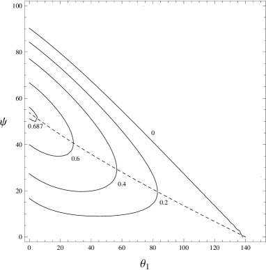
(a)	(b)

Figure 2: (a) The dependence of the maximal distance $d_{m}$ from the sphere to the plane on the contact angle $\theta_{2}$ for $\theta_{1}=0$. (b) The solutions of the equation (3.4) for $\theta_{2}=40^{o}$ for different values of the distance $d$ from the sphere to the plane. The dashed curve shows the position of the degenerate ${\sf Cat}$ menisci.

There exists a single nonzero value of the filling angle $\psi$ satisfying equation (3.4) at $d=0$ that leads to the Plateau sequence (see Figure 3(a)). Catenoid cannot be observed for $d>d_{m}$, but there exists a range of distances $0<d<d_{m}$ for which equation (3.4) is satisfied for two values of the filling angle as shown in Figure 3(c). The corresponding sequence of menisci looks like

$${\sf Und_{0}^{-}}\rightarrow{\sf Cat}\rightarrow{\sf Nod^{-}}\rightarrow{\sf Cat}\rightarrow{\sf Und_{0}^{-}}\rightarrow{\sf Und_{1}^{-}}\rightarrow{\sf Und_{0}^{+}}\rightarrow{\sf Sph^{+}_{0}}\rightarrow{\sf Nod^{+}}\;.$$

The sequence of menisci can pass through a single catenoid but it differs from the Plateau type as shown in Figure 3(d). This occurs in the degenerated case when equation (3.4) has to be complemented by an additional requirement: $\partial\theta_{1}/\partial\psi=0$. Taking derivatives with respect to $\psi$ in both sides of equation (3.4) and applying the above condition we arrive at a trigonometric equation

$$2\sin\psi=\left(\ln\cot\frac{\theta_{1}+\psi}{2}+\ln\cot\frac{\theta_{2}}{2}\right)\sin(\theta_{1}+2\psi)\;.$$ (3.7)

Solution of equation (3.7) for fixed $\theta_{2}$ determines a curve $\theta_{1}(\psi)$ on which the degenerated ${\sf Cat}$ meniscus appears. It is shown in Figure 2(b) by dashed curve.

(a)	(b)
(c)	(d)

Figure 3: The case (a) presents the typical curve at $d=0$ with $\theta_{1}=30^{o}$, $\theta_{2}=80^{o}$, discussed in [5], while the case (b) at $d=0$ with $\theta_{1}=120^{o}$, $\theta_{2}=90^{o}$, characterized by a requirement $\theta_{1}+\theta_{2}>\pi$, was not considered in [5]. For positive distance $d>0$ one observes (c) with $d=0.4$ with $\theta_{1}=\theta_{2}=40^{o}$ two catenoids that degenerate for larger distance into a single catenoid (d) with $d=0.53$. Different colors indicate the menisci of different types: ${\sf Und^{-}_{1}}$ (red), ${\sf Und^{-}_{0}}$ (cyan), ${\sf Und^{+}_{0}}$ (green), ${\sf Nod^{-}}$ and ${\sf Nod^{+}}$ (black). They correspond to colors of types shown in Figure 6.

3.2 Unduloids ($c<0$)

Before starting to treat the unduloidal solution of equation (2.10) it is worth to make

Remark 1

Equation (2.1) with boundary conditions is associated with nonlinear eigenvalue problem and in the case of unduloids its solution has a discrete spectrum and, therefore, is enumerated by two indices. The first integer non-negative index $n$ determines the number of the inflection points on the meniscus meridional profile. When the part of this profile touching the solid sphere is convex the second integer index $s$ takes value of $1$, otherwise it equals to $-1$. Thus, the unduloid meniscus is denoted as ${\sf Und_{n}^{s}}$.

The existence of the ${\sf Und_{n}^{s}}$ meniscus requires satisfaction of the condition $\sin^{2}t+c\geq 0$ for $t\in\{t_{2},t_{1}\}$. This condition is rewritten in the form

$$\sin^{2}t\geq[1-(1-2\alpha)^{2}]\sin^{2}t_{1}\;.$$ (3.8)

Denote $\sin t_{m}=\min(\sin t_{1},\sin t_{2})$. The last condition leads to $\sin^{2}t_{m}\geq[1-(1-2\alpha)^{2}]\sin^{2}t_{1}$, and yields

$$\alpha\leq\beta^{-}(\psi),\quad\alpha\geq\beta^{+}(\psi),\quad\mbox{where}\quad\beta^{\pm}(\psi)=\frac{1}{2}\left(1\pm\sqrt{1-\sin^{2}t_{m}/\sin^{2}t_{1}}\right).$$ (3.9)

The restrictions (3.9) define in the plane $\{\psi,\alpha\}$ a new object ${\mathbb{B}}$ which we called a balloon. It comprises an oval and two additional lines $\alpha=1/2$ (see detailed description in section 5). Hereafter the balloon ${\mathbb{B}}$ becomes a main tool of our study the dependence $\alpha(\psi)$. In regard to $H(\psi)$ the balloon undergoes the non linear transformation (2.8). In Figure 4 we present both dependencies $H_{n}(\psi)$ and $\alpha_{n}(\psi)$ with the balloon ${\mathbb{B}}$.

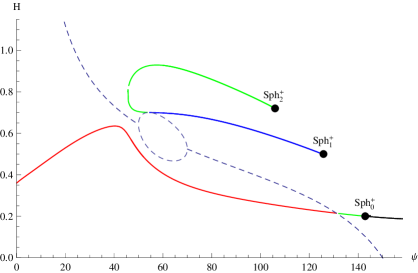
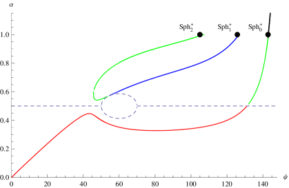
(a)	(b)

Figure 4: The dependencies $H_{n}(\psi)$ in (a) and $\alpha_{n}(\psi)$ in (b) for $\theta_{1}=30^{o}$, $\theta_{2}=80^{o}$ and $d=2.3$ with two disjoined curves. The balloon ${\mathbb{B}}$ is shown by dashed line. Spherical menisci ${\sf Sph^{+}_{0}}$, ${\sf Sph^{+}_{1}}$ and ${\sf Sph^{+}_{2}}$ are denoted by black dots. The curve segments correspond to colors of the menisci types shown in Figure 6.

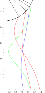
(a)	(b)	(c)

Figure 5: The menisci ${\sf Und^{-}_{1}}$ (red), ${\sf Und^{+}_{1}}$ (green), and ${\sf Und^{+}_{2}}$ (blue) for $\theta_{1}=30^{o}$, $\theta_{2}=80^{o}$ and $d=2.2$ computed in three different setups: (a) for $\psi=60^{o}$ they have different volumes $V$ and surface areas $S$; (b) for fixed $V=3.6$ there are 4 menisci with $\psi_{1}=34^{o}$ and $\psi_{2}=47.2^{o}$ – ${\sf Und^{-}_{1}}$, $\psi_{3}=61.7^{o}$ – ${\sf Und^{+}_{1}}$, $\psi_{4}=71.3^{o}$ – ${\sf Und^{+}_{2}}$ and different surface areas $S$; (c) for fixed $S=11.3$ there are 4 profiles with $\psi_{1}=30.3^{o}$ and $\psi_{2}=47.1^{o}$ – ${\sf Und^{-}_{1}}$, $\psi_{3}=56.7^{o}$ – ${\sf Und^{+}_{1}}$, $\psi_{4}=61.95^{o}$ – ${\sf Und^{+}_{2}}$ and different volumes $V$.

The relations (3.9) are independent of distance $d$ and remain valid for all types of inflectional unduloids with $0<\alpha<1$. For all unduloids they define the restrictions on the curvature values that can be obtained using the definition (2.8). On the other hand, these relations correspond to a single condition on $c$ value

$$-\sin^{2}t_{m}\leq c\leq 0.$$ (3.10)

In Figure 5 we present three families of unduloid menisci for fixed filling angle $\psi$ (Figure 5(a)), volume $V$ (Figure 5(b)) and surface area $S$ (Figure 5(c)) of pendular ring.

3.3 Nodoids ($c>0$)

The ${\sf Nod}$ meniscus has positive $c$ irrespectively to its concave or convex version. Therefore the above analysis of $\alpha$ fails and it is replaced by another one, less strong but still universal.

Show that for $d>0$ the ${\sf Nod^{s}}$ menisci satisfy the following constraints,

$$H(\psi,0)<H(\psi,d)<0\quad({\sf Nod^{-}}),\quad\quad 0<H(\psi,d)<H(\psi,0)\quad({\sf Nod^{+}})\;,$$ (3.11)

using (3.1) and several additional observations listed below.

First, the curvature $H$ for any finite $d$ is always negative for the ${\sf Nod^{-}}$ meniscus and always positive for the ${\sf Nod^{+}}$ meniscus. Next, the ${\sf Nod^{-}}$ meniscus disappears at finite $d$ when two catenoids annihilate. Finally, when $\psi\to\pi$ and $d\to\infty$ the curvature of the ${\sf Nod^{+}}$ meniscus tends to zero. Combining these facts with (3.1) we arrive at constraints (3.11).

The main statement stemming from (3.11) is that the two different curves $H(\psi,d_{1})$ and $H(\psi,d_{2})$, $d_{1}\neq d_{2}$, do not intersect in the entire angular $\psi$ range of the ${\sf Nod^{-}}$ and ${\sf Nod^{+}}$ menisci existence. Although this statement is of high (topological) importance, it does not provide the quantitative estimates. Therefore for the ${\sf Nod^{-}}$ meniscus we give one more estimate for the curvature.

Start with relationship between the curvature $H$ and the surface area $S$ for ${\sf Nod^{-}}$ meniscus. For this purpose combine formulas (2.10, 2.11, 2.13, 2.14, 2.19) and obtain

$$\frac{2H^{2}}{\pi}S=K_{-}=2(I_{1}-I_{2})-I_{3}=4H\Psi-I_{3}\;.$$ (3.12)

Keeping in mind the positiveness of $S$ we arrive at the bound $4H\Psi\geq I_{3}$. Using the definition (2.16) we obtain $I_{3}\geq-\delta\sqrt{c}$, where $\delta=\pi-\theta_{1}-\theta_{2}-\psi$, $\delta\geq 0$. Thus, substituting this relation in the above inequality we find

$$H\geq-\frac{\delta}{4\Psi}\sqrt{c}\;.$$ (3.13)

This bound does not contradict inequalities (3.11) for the ${\sf Nod^{-}}$ meniscus since its curvature is negative. Keeping in mind this fact and substituting (2.7) into (3.13) we arrive at

$$H\geq\frac{\sin\psi\;\sin(\theta_{1}+\psi)}{\sin^{2}\psi-4\Psi^{2}\delta^{-2}}\;.$$ (3.14)

This inequality is equivalent to

$$\alpha\geq\frac{\delta^{2}\sin^{2}\psi}{\delta^{2}\sin^{2}\psi-4\Psi^{2}}\;.$$ (3.15)

The last inequalities have one important consequence. Since $H<0$ then the necessary condition for the ${\sf Nod^{-}}$ meniscus existence is

$$\delta\sin\psi<2\Psi\Rightarrow\frac{\pi-\theta_{1}-\theta_{2}-\psi}{2}\sin\psi+\cos\psi<1+d.$$ (3.16)

For convex nodoid ${\sf Nod^{+}}$ meniscus it is possible to find explicit expression for the upper bound $H(\psi,0)$. First, note that as it is demonstrated in Appendix C meniscus curvature has a local minimum, so that the upper bound is given by the largest of two curvature values – $H(\phi_{0}^{+})$ at the sphere ${\sf Sph_{0}^{+}}$ and $H(\pi)$ at $\psi=\pi$. These values are

$$H(\phi_{0}^{+})=\frac{\sin(\theta_{1}+\phi_{0}^{+})}{\sin\phi_{0}^{+}},\quad H(\pi)=\frac{1-\cos\theta_{2}}{2+d}.$$

Show that $H(\phi_{0}^{+})>H(\pi)$. Indeed, this condition implies

$$(1+d)\sin(\theta_{1}+\phi_{0}^{+})+\cos\theta_{2}\sin\phi_{0}^{+}>\sin\phi_{0}^{+}-\sin(\theta_{1}+\phi_{0}^{+}).$$

Using in the above relation the l.h.s. of formula (B.9) we obtain

$$\sin\theta_{1}>\sin\phi_{0}^{+}-\sin(\theta_{1}+\phi_{0}^{+}),$$

leading to

$$\cos\frac{\theta_{1}}{2}+\cos\left(\phi_{0}^{+}+\frac{\theta_{1}}{2}\right)=\cos\frac{\theta_{1}+\phi_{0}^{+}}{2}\cos\frac{\phi_{0}^{+}}{2}>0.$$ (3.17)

Recalling that $\theta_{1}+\phi_{0}^{+}<\pi$ we see that (3.17) is always valid. Thus, the upper bound for the ${\sf Nod^{+}}$ meniscus is given by $H(\phi_{0}^{+},0)$. To find this value explicitly we use (B.9) with $n=0$ and $d=0$ to produce

$$\sin(\theta_{1}+\phi_{0}^{+})+\cos\theta_{2}\sin\phi_{0}^{+}-\sin\theta_{1}=0\Rightarrow\cos\left(\theta_{1}+\frac{\phi_{0}^{+}}{2}\right)+\cos\theta_{2}\cos\frac{\phi_{0}^{+}}{2}=0.$$

The last relation implies

$$\tan\frac{\phi_{0}^{+}}{2}=\frac{\cos\theta_{1}+\cos\theta_{2}}{\sin\theta_{1}}.$$ (3.18)

On the other hand, we have

$$H(\phi_{0}^{+},0)=\frac{\sin(\theta_{1}+\phi_{0}^{+})}{\sin\phi_{0}^{+}}=\cos\theta_{1}+\sin\theta_{1}\cot\phi_{0}^{+}.$$

Using (3.18) in last expression we find for the upper bound of ${\sf Nod^{+}}$ meniscus

$$H(\phi_{0}^{+},0)=\frac{\sin^{2}\theta_{2}}{2(\cos\theta_{1}+\cos\theta_{2})}.$$ (3.19)

3.4 Spheres ($c=0$)

The spheres can be considered as a limiting case of the unduloid menisci and, therefore, also labeled by two indices ${\sf Sph^{s}_{n}}$. Consider a function

$$f_{n}(\psi)=(1+d)\sin(\theta_{1}+\psi)-(n-\delta)\sin\psi-\sin\theta_{1},$$ (3.20)

which root $\psi=\phi_{n}^{+}$ satisfying the equation $f_{n}(\phi_{n}^{+})=0$ provides the value of the filling angle at which sphere ${\sf Sph^{+}_{n}}$ is observed (see (B.9)). In (3.20) one has $\delta=0$ for odd $n$ and $\delta=\cos\theta_{2}$ for even $n$. It is easy to check that

$$f_{n+1}(\psi)-f_{n}(\psi)=-[1+\cos\pi n\cos\theta_{2}]\sin\psi<0,$$

which means that the curve $f_{n+1}$ lies below the curve $f_{n}$.

The value of the function $f_{n}$ at $\psi=0$ reads $f_{n}(0)=d\sin\theta_{1}$ which is non-negative, while $f_{n}(\pi)=-(2+d)\sin\theta_{1}$ is always negative. Noting that the function $f_{n}$ is a periodic one with the period $2\pi$ we find that for positive $d$ in the interval $\{0,\pi\}$ the function $f_{n}$ has a single root $\phi_{n}^{+}$ and $f_{n}^{\prime}(\phi_{n}^{+})<0$. As $f_{n+1}(\phi_{n}^{+})<f_{n}(\phi_{n}^{+})=0$ and $f_{n+1}^{\prime}(\phi_{n+1}^{+})<0$ we immediately find that $\phi_{n+1}^{+}<\phi_{n}^{+}$. This means that for positive $d$ the value $\psi_{n}$ of the filling angle at which sphere ${\sf Sph^{+}_{n}}$ is observed decreases with increase of $n$. For very large $n$ the value of $\phi_{n}^{+}$ tends to zero. Using (3.20) we find in linear approximation

$$\sin\phi_{n}^{+}=\phi_{n}^{+}=\frac{d\sin\theta_{1}}{n-\delta-\cos\theta_{1}}\approx\frac{d\sin\theta_{1}}{n},\ \ \ n\gg 1.$$ (3.21)

For $d\leq 0$ we have $f_{n}(0)\leq 0$ and the first derivative reads $f^{\prime}_{n}(0)=\cos\theta_{1}-(n-\delta)$. For $n>0$ this derivative is negative, so that the function $f_{n}$ has no roots. When $n=0$ we have $f^{\prime}_{0}(0)=\cos\theta_{1}+\cos\theta_{2}$. This expression is negative for $\theta_{1}+\theta_{2}>\pi$, so that no spheres exist for $d=0$ when the last condition holds. Finally, in case of the wetting sphere $\theta_{1}=0$ we have $f_{n}(0)=f_{n}(\pi)=0$ and no spheres are allowed to exist.

Show that for fixed $n$ the value $\phi_{n}^{+}(d)$ of the filling angle of sphere ${\sf Sph^{+}_{n}}$ increases with growing $d$. Indeed, from (3.20) one finds that the difference

$$f_{n}(\phi_{n}^{+}(d),d_{1})-f_{n}(\phi_{n}^{+}(d),d)=(d_{1}-d)\sin(\theta_{1}+\phi_{n}^{+}(d)),$$

is positive for $d_{1}>d$. As $f_{n}^{\prime}(\phi_{n}^{+})<0$ it immediately follows that $\phi_{n}^{+}(d_{1})>\phi_{n}^{+}(d)$.

Another type of sphere ${\sf Sph^{-}_{n}}\;(n>0)$ discussed in B.2 can be considered as a limiting shape of the ${\sf Und^{-}_{n}}$ meniscus at $\psi\to 0$, its curvature is given by (B.8).

In Table 1 the characteristic signs of $H$, $c$ are given for different types of menisci.

Table 1.

$$\begin{array}[]{|c|c|c|c|c|c|c|c|}\hline\cr&{\sf Nod^{-}}&{\sf Cat}&{\sf Und_{n}^{s}}&{\sf Cyl}&{\sf Sph_{n}^{s}}&{\sf Nod^{+}}\\ \hline\cr\hline\cr H&-&0&+&+&+&+\\ \hline\cr c&+&0&-&-&0&+\\ \hline\cr\end{array}$$

Note that the meniscus ${\sf Und_{n}^{s}}$ comes in several different types depending on the number $n$ of inflection points and the curvature of the segment of meridional profile is touching the sphere: $s=-1$ for concave profile and $s=+1$ for convex one.

4 Unduloid Menisci Transitions

Transitions between unduloids and nodoids of different types can be easily classified. Namely, there exist transitions between the concave ${\sf Und_{0}^{-}}$ (convex ${\sf Und_{0}^{+}}$) unduloid to concave ${\sf Nod^{-}}$ (convex ${\sf Nod^{+}}$) nodoid through catenoid ${\sf Cat}$ (sphere ${\sf Sph^{+}_{0}}$). The transitions between different types of unduloids are numerous and schematically presented in Figure 6.

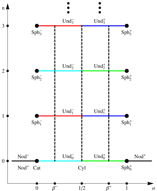
Figure 6: Possible transitions between menisci of different types shown as a function of the parameter $\alpha$. The left vertical dashed line represents the transitions at $\alpha=\beta^{-}$ between ${\sf Und_{n}^{-}}$ unduloids. Similarly, the right vertical dashed line corresponds to the transitions at $\alpha=\beta^{+}$ between ${\sf Und_{n}^{+}}$ unduloids. Finally, the transitions between unduloids of opposite signs takes place at $\alpha=1/2$ and is represented by the central vertical dashed line.

As shown in A.7 and A.8 all inflection points for a given inflectional unduloid ${\sf Und_{n}^{s}}$ have the same abscissa value $x_{\ast}=\sin t_{\ast}^{s}/(2H)=\sqrt{-c}/(2H)$. An addition (removal) of an inflection point may take place only as the result of the inflection point separation from (merging with) the sphere or the plane. When the inflection point is on the sphere we have $c+\sin^{2}t_{1}=0$ to obtain using (A.16)

$$2H\sin\psi=\sin t_{1}.$$

Recalling definition (2.8) we find $\alpha=1/2$. Noting that menisci ${\sf Und_{n}^{-}}$ (${\sf Und_{n}^{+}}$) exist at $\alpha\leq 1/2$ ($\alpha\geq 1/2$) we find that transitions of the type ${\sf Und_{n}^{s}}\leftrightarrow{\sf Und_{n\pm 1}^{-s}}$ occur at $\alpha=1/2$ when the inflection point is on the sphere. For the inflection point on the plane we have $c+\sin^{2}t_{2}=0$ to obtain with (A.17)

$$2H\sin\psi=\sin t_{1}+s\sqrt{\sin^{2}t_{1}-\sin^{2}t_{2}}\;,$$

and we find using (3.9) that in this case the transitions of the type ${\sf Und_{n}^{s}}\leftrightarrow{\sf Und_{n\pm 1}^{s}}$ occur at $\alpha=\beta^{s}$.

Menisci of the ${\sf Und_{n}^{+}}$ type exist for $1/2<\alpha<1$. With growth of $\alpha$ the abscissa of the leftmost point of the meniscus meridional section tends to zero and reaches it at $\alpha=1$. At this moment the profile is made of several segments of a circle and the meniscus touches the axis of rotation $x=0$. The spherical menisci ${\sf Sph_{n}^{+}}$ at $\alpha=1$ are described in B.1.

The above considerations lead to the following rules of transition between unduloids:

$$\begin{array}[]{ccc}{\sf Und_{n}^{s}}\longleftrightarrow{\sf Und_{n\pm 1}^{s}}&\mbox{at}&\alpha=\beta^{s},\\ {\sf Und_{n}^{s}}\longleftrightarrow{\sf Und_{n\pm 1}^{-s}}&\mbox{at}&\alpha=1/2.\end{array}$$

Thus we show that the balloon introduced above can be viewed as a set of transition points between unduloids.

Show that for fixed values of $\theta_{1},\theta_{2}$ and $d$ the curves corresponding to different unduloid types never intersect (except for the transition points discussed above that arises in case when the unduloid orders differ by unity). As the curves corresponding to unduloids of opposite signs cannot intersect in $\{\psi,\alpha\}$ plane, we have to consider only unduloids of the same sign.

Consider first same sign unduloids of the orders that differ by an even number, for example, ${\sf Und_{2k}^{s}}$ and ${\sf Und_{2k^{\prime}}^{s}}$, or ${\sf Und_{2k+1}^{s}}$ and ${\sf Und_{2k^{\prime}+1}^{s}}$, where $k\neq k^{\prime}$. It immediately follows from (A.46) and (A.52) that the difference between the curvatures of these menisci is $(k-k^{\prime})\hat{I}_{2}/\Psi\neq 0$.

If the order difference is odd and larger than two we have for unduloids ${\sf Und_{2k}^{s}}$ and ${\sf Und_{2k^{\prime}+1}^{s}}$ with $k^{\prime}\neq k$, the curvature difference reads $[(k^{\prime}-k)\hat{I}_{2}+I_{2}(t_{\ast}^{s},t_{2})]/\Psi$. Consider the integrals $I_{2}(t_{\ast}^{s},t_{2})$ which are finite and real. Note that $t_{\ast}^{+}<t_{2}<t_{\ast}^{-}$, which leads to

$$|I_{2}(t_{\ast}^{s},t_{2})|<I_{2}(t_{\ast}^{-},t_{\ast}^{+})=\hat{I}_{2}.$$

The last relation implies that the curvature differences mentioned above are nonzero that finishes the proof.

From (B.7) it follows that the curvature of spherical menisci ${\sf Sph^{+}_{n}}$ grows monotonically with order increase without any restriction to the order value. This means also that the corresponding unduloids ${\sf Und_{n}^{+}}$ can be observed without any restrictions to the order $n$.

The asymptotic behavior of the curvature at small filling angles $\psi\ll 1$ is discussed in Appendix B.1. For $d>0$ at zero filling angle $\psi=0$ only concave unduloids ${\sf Und_{n}^{-}}\;(n>0)$ exist. From (B.8) it follows that for $n=0$ the curvature $H(0)=0$ leading to contradiction as the curvature can turn to zero only for catenoid. It is important to underline that there are no other restrictions to existence of ${\sf Und_{n}^{-}}\;(n>0)$ unduloids at zero filling angle.

Using the formula (A.58) for unduloid curvature we have

$$2H_{n}^{s}\Psi=I_{1}(t_{1},t_{2})+sI_{2}(t_{1},t_{2})+n\hat{I}_{2}-s(1-\cos\pi n)I_{2}(\pi/2,t_{2}),\quad s=\mbox{sgn}(2\alpha_{n}-1)\;,$$ (4.1)

where the sign $s=\pm 1$ corresponds to two menisci which differ by the sign of the meridional curvature at the meniscus-sphere contact point. Equation (4.1) defines the function $\alpha_{n}(\psi)$ in two different regions, $\alpha_{n}>1/2$ and $\alpha_{n}<1/2$, while $\alpha_{n}(\psi)$ is a smooth at $\alpha_{n}=1/2$.

Rewrite (4.1) as follows, $\Phi_{n}^{s}(\alpha_{n},\psi)=0$, where

$$\Phi_{n}^{s}(\alpha_{n},\psi)=-2\alpha_{n}\Psi\sin t_{1}+\left[I_{1}(t_{1},t_{2})+sI_{2}(t_{1},t_{2})+n\hat{I}_{2}-s(1-\cos\pi n)I_{2}(\pi/2,t_{2})\right]\sin\psi,$$ (4.2)

One can define the derivative $\alpha^{\prime}_{n}(\psi)$ having a unique value determined from the equation

$$A_{n}^{s}\alpha^{\prime}_{n}(\psi)+B_{n}^{s}=0,\ \ \ A_{n}^{s}=\frac{\partial\Phi_{n}^{s}}{\partial\alpha_{n}},\ \ \ B_{n}^{s}=\frac{\partial\Phi_{n}^{s}}{\partial\psi},$$ (4.3)

where the both functions $A_{n}^{s}(\alpha_{n},\psi)$ and $B_{n}^{s}(\alpha_{n},\psi)$ do not vanish simultaneously.

Direct computation gives the following expressions for $A_{n}^{s}(\alpha_{n},\psi)$ and $B_{n}^{s}(\alpha_{n},\psi)$

$$A_{n}^{s}(\alpha_{n},\psi) = -2\Psi\sin t_{1}-$$ (4.4)

$$2(2\alpha_{n}-1)\sin^{2}t_{1}\sin\psi\left[sI_{4}(t_{1},t_{2})-2n\hat{I}_{2}^{\prime}(c)-s(1-\cos\pi n)I_{4}(\pi/2,t_{2})\right],\hskip 22.76228pt$$

$$B_{n}^{s}(\alpha_{n},\psi) = 2\alpha_{n}\Psi\frac{\sin\theta_{1}}{\sin\psi}-\frac{4\alpha_{n}^{2}-2\alpha_{n}-1}{2\alpha_{n}-1}\sin t_{1}\sin\psi+\sin^{2}\psi-$$ (4.5)

$$2\alpha_{n}(\alpha_{n}-1)\sin 2t_{1}\sin\psi\left[sI_{4}(t_{1},t_{2})-2n\hat{I}_{2}^{\prime}(c)-s(1-\cos\pi n)I_{4}(\pi/2,t_{2})\right],$$

where the integral $I_{4}(t_{1},t_{2})$ is computed in (2.24) and the derivative $\hat{I}_{2}^{\prime}(c)$ is given by (D.13).

4.1 Transitions ${\sf Und_{n}^{-}}\leftrightarrow{\sf Und_{n+s}^{+}}$

Consider first the transitions on the line $\alpha=1/2$ between unduloids of opposite signs. This transition takes place when the point $t_{1}=t_{\ast}^{s}$ separates from the sphere, where $t_{\ast}^{+}=\arcsin\sqrt{-c}$ and $t_{\ast}^{-}=\pi-\arcsin\sqrt{-c}$. As $H=\sin t_{1}/(2\sin\psi)$ we use (4.1) to obtain

$$\Psi\sqrt{-c}=\left[I_{1}(t_{\ast}^{s},t_{2})-I_{2}^{\ast}(t_{\ast}^{s},t_{2})+n\hat{I}_{2}+(1-\cos\pi n)I_{2}(\pi/2,t_{2})\right]\sin(t_{\ast}^{s}-\theta_{1}),$$ (4.6)

where we introduce a special case of the integral $I_{2}$

$$I_{2}^{\ast}(t_{1},t_{2})=\int_{t_{2}}^{t_{1}}\frac{\sin^{2}t\;dt}{\sqrt{\sin^{2}t-\sin^{2}t_{1}}}.$$ (4.7)

The general expressions for the abscissa of the meniscus meridional profile contain the term $\sqrt{\sin^{2}t+c}$, which at the transition point transforms into $\sqrt{\sin^{2}t-\sin^{2}t_{\ast}^{\pm}}$. It leads to a condition $t_{2}<t_{\ast}^{-}$ producing

$$\begin{array}[]{lcll}t_{2}<\pi-t_{1}&\longrightarrow&\psi<\theta_{2}-\theta_{1},&s=+1,\\ t_{2}<t_{1}&\longrightarrow&\psi>\pi-\theta_{2}-\theta_{1},&s=-1,\end{array}$$

implying that the transition takes place to the left (right) of the balloon for $s=1$ ($s=-1$).

Show that the transition considered in this subsection is smooth, i.e., unduloids ${\sf Und_{n}^{-}}$ and ${\sf Und_{n+s}^{+}}$ meet smoothly at $\alpha=1/2$. It means that the value of the derivative $\alpha^{\prime}(\psi)$ computed on both sides of the transition point is the same. As at the transition point we have $c+\sin^{2}t_{1}=0$ the integral $I_{4}(t_{1},t_{2})$ in (4.4,4.5) diverges. We show below that nevertheless both $A$ and $B$ have finite value at the transition point. In the vicinity of $\alpha=1/2$ we introduce $\alpha=1/2+s\epsilon$ and find $c=(4\epsilon^{2}-1)\sin^{2}t_{1}$ and $\sqrt{c+\sin^{2}t_{1}}=2\epsilon\sin t_{1}$. Making use of (2.24) decompose the integral $I_{4}(t_{1},t_{2})$ into diverging $I_{4d}(t_{1},t_{2})$ and non-diverging $I_{4c}(t_{1},t_{2})$ parts,

$$I_{4}(t_{1},t_{2})=I_{4c}(t_{1},t_{2})+I_{4d}(t_{1},t_{2})\;,\quad I_{4d}(t_{1},t_{2})=-\frac{1}{s(2\alpha-1)\cos t_{1}}\;.$$ (4.8)

Using this relation in (4.4) we find

$$A_{n}^{s}=-2\Psi\sin t_{1}-\frac{2\sin^{2}t_{1}\sin\psi}{\cos t_{1}}=2\tan t_{1}[\cos\theta_{1}-(1+d)\cos t_{1}].$$ (4.9)

Substitute (4.8) into (4.5) and note that two diverging terms cancel each other in vicinity of $\alpha=1/2$,

$$- \frac{4\alpha^{2}-2\alpha-1}{2\alpha-1}\sin t_{1}\sin\psi-2s\alpha(\alpha-1)\sin 2t_{1}\sin\psi I_{4d}(t_{1},t_{2})$$

$$= \frac{1}{2\alpha-1}\sin t_{1}\sin\psi-\frac{1}{2(2\alpha-1)}\frac{\sin 2t_{1}\sin\psi}{\cos t_{1}}=0.$$

The remaining terms read

$$B_{n}^{s}=\Psi\frac{\sin\theta_{1}}{\sin\psi}+\sin^{2}\psi+\sin t_{1}\cos t_{1}\sin\psi\left[sI_{4c}(t_{1},t_{2})-2n\hat{I}_{2}^{\prime}(c)-s(1-\cos\pi n)I_{4}(\pi/2,t_{2})\right].$$

Show that this expression is conserved at the transition ${\sf Und_{n}^{-}}\leftrightarrow{\sf Und_{n+s}^{+}}$. It is sufficient to show that it is valid for the expression in the square brackets in (4.11) that leads to the relation

$$I_{4c}(t_{1},t_{2})-I_{4}(\pi/2,t_{2})=s_{1}\hat{I}_{2}^{\prime}(c),$$

where $s_{1}=1$ ($s_{1}=-1$) corresponds to the transition to the left (right) of the balloon with $t_{1}=t_{\ast}^{s_{1}}$. The last relation can be written as follows:

$$I_{4c}(t_{\ast}^{s_{1}},\pi/2)=s_{1}\hat{I}_{2}^{\prime}(c),$$ (4.10)

It is easy to see that

$$I_{4c}(t_{\ast}^{s},\pi/2)=I_{4c}(\pi/2,\pi-t_{\ast}^{s})=\frac{1}{2}I_{4c}(t_{\ast}^{s},\pi-t_{\ast}^{s}),$$

and using (D.19) we establish the validity of (4.10). Thus we find at $\alpha=1/2$

$$B_{n}^{s}=\Psi\frac{\sin\theta_{1}}{\sin\psi}+\sin^{2}\psi-\sin t_{1}\cos t_{1}\sin\psi[(2n-ss_{1})\hat{I}_{2}^{\prime}(c)-s\cos\pi n\;I_{4}(\pi/2,t_{2})].$$ (4.11)

Selecting here $s=-1$ we arrive at the final expression for $B$

$$B_{n}^{-}=\Psi\frac{\sin\theta_{1}}{\sin\psi}+\sin^{2}\psi-\sin t_{1}\cos t_{1}\sin\psi[(2n+s_{1})\hat{I}_{2}^{\prime}(c)+\cos\pi n\;I_{4}(\pi/2,t_{2})],$$ (4.12)

where $s_{1}=1$ ($s_{1}=-1$) corresponds to the transition ${\sf Und_{n}^{-}}\leftrightarrow{\sf Und_{n+s_{1}}^{+}}$ to the left (right) of the balloon.

4.2 Transitions ${\sf Und_{n}^{s}}\leftrightarrow{\sf Und_{n+1}^{s}}$

This transition for odd $n$ takes place at $\alpha=\beta^{s}=(1+s\sqrt{1+c/\sin^{2}t_{1}})/2$ when the point $t_{2}=t_{\ast}^{-s}$ separates from the plane and we obtain

$$2H_{n}^{s}\Psi=I_{1}(t_{1},t_{\ast}^{-s})+sI_{2}(t_{1},t_{\ast}^{-s})+(n+1)\hat{I}_{2}.$$ (4.13)

As $c=-\sin^{2}t_{2}$ we find

$$I_{2}(t_{1},t_{2})=\int_{t_{2}}^{t_{1}}\frac{\sin^{2}t}{\sqrt{\sin^{2}t-\sin^{2}t_{2}}}=-\int_{t_{1}}^{t_{2}}\frac{\sin^{2}t}{\sqrt{\sin^{2}t-\sin^{2}t_{2}}}=-I_{2}^{\ast}(t_{2},t_{1}),$$ (4.14)

and arrive at

$$\Psi=\left[I_{1}(t_{1},t_{\ast}^{-s})-sI_{2}^{\ast}(t_{\ast}^{-s},t_{1})+(n+1)\hat{I}_{2}\right]\frac{\sin\psi}{2\beta^{s}\sin t_{1}}.$$

For even $n$ this transition is observed with separation of the point $t_{2}=t_{\ast}^{s}$ from the plane for which we obtain

$$\Psi=\left[I_{1}(t_{1},t_{\ast}^{s})-sI_{2}^{\ast}(t_{\ast}^{s},t_{1})+n\hat{I}_{2}\right]\frac{\sin\psi}{2\beta^{s}\sin t_{1}}.$$

Discuss one more question: how smooth are transitions ${\sf Und_{n}^{+}}\leftrightarrow{\sf Und_{n+1}^{+}}$ at upper ($\alpha=\beta^{+}$) and ${\sf Und_{n}^{-}}\leftrightarrow{\sf Und_{n+1}^{-}}$ at lower ($\alpha=\beta^{-}$) arcs of balloon, respectively. To this end, consider equation (4.3) in vicinity of the transition point ($\psi_{*},\beta^{s}(\psi_{*})$) belonging to the balloon and estimate the leading terms in (4.4) and (4.5) when $c\to-\sin^{2}t_{2}$. The only divergent terms are integrals $I_{4}(t_{1},t_{2})$ and $I_{4}(\pi/2,t_{2})$ which by (2.24) behave as follows,

$$I_{4}(t_{1},t_{2}),I_{4}(\pi/2,t_{2})\stackrel{{\scriptstyle c+\sin^{2}t_{2}\;\to\;0}}{{\simeq}}\frac{\sin 2t_{2}}{2(1+c)\sqrt{\sin^{2}t_{2}+c}}.$$ (4.15)

Substituting (4.15) into (4.4) and (4.5) we arrive in the limiting case $c+\sin^{2}t_{2}\to 0$ to explicit formula

$$\alpha^{\prime}(\psi_{*})=\frac{2\beta^{s}(\beta^{s}-1)}{2\beta^{s}-1}\cot(\theta_{1}+\psi_{*}),$$ (4.16)

which is finite for $\beta^{s}\neq 1/2$ and independent on order $n$, i.e., both curves ${\sf Und_{n}^{s}}$ and ${\sf Und_{n+1}^{s}}$ meet smoothly at the balloon.

4.3 Transitions ${\sf Und_{1}^{-}}\leftrightarrow{\sf Und_{1}^{+}}$, ${\sf Und_{2n}^{-}}\leftrightarrow{\sf Und_{2n}^{+}}$ and ${\sf Und_{2n}^{-}}\leftrightarrow{\sf Und_{2n+2}^{+}}$

In previous sections we have discussed in details conditions and rules of regular transitions between unduloids that accompanied by addition or removal of one inflection point. It is also possible to observe degenerate transitions when the number of inflection points changes by two or does not change at all. Find the conditions for such degenerate transitions.

An addition of two inflection points takes place only when one of these points separates from the solid sphere and the other one from the plane. The first event corresponds to a condition $c+\sin^{2}t_{1}=0$, while the second one requires $c+\sin^{2}t_{2}=0$. These relations imply $\sin t_{1}=\sin t_{2}$ leading to $\psi_{1}^{\ast}=\min\{\theta_{2}-\theta_{1},\pi-\theta_{1}-\theta_{2}\}$ and $\psi_{2}^{\ast}=\max\{\theta_{2}-\theta_{1},\pi-\theta_{1}-\theta_{2}\}$. These critical values define the extremal points of the balloon where it transforms into the segments of the line $\alpha=1/2$. When $\psi_{1}^{\ast}$ is negative only a part of the balloon is observed. When both values $\psi_{i}^{\ast}$ are negative the balloon does not exists. Finally, for $\theta_{2}=\pi/2$ the balloon reduces to a point at $\psi^{\ast}=\pi/2-\theta_{1}$.

Consider the transition ${\sf Und_{2k}^{-}}\leftrightarrow{\sf Und_{2k+2}^{+}}$ at $\psi=\psi_{1}^{\ast}$. Using (A.46) and noting that $t_{1}=\theta_{2}=t_{\ast}^{-}$ we find

$$\frac{\sin\theta_{2}}{\sin\psi}\Psi=I_{1}(\theta_{2},\pi-\theta_{2})-I_{2}(\theta_{2},\pi-\theta_{2})+2k\hat{I}_{2}=-2\cos\theta_{2}+(2k+1)\hat{I}_{2},$$

from which we obtain the distance $d_{n}$ where this transition occurs

$$d_{n}=-1+\cos(\theta_{2}-\theta_{1})+\frac{\sin(\theta_{2}-\theta_{1})}{\sin\theta_{2}}\;\left[(n+1)\hat{I}_{2}-2\cos\theta_{2}\right].$$ (4.17)

The case $k=0$ should formally correspond to the transition ${\sf Und_{0}^{-}}\leftrightarrow{\sf Und_{2}^{+}}$. It can be checked that ${\sf Und_{0}^{-}}$ unduloid can exist only below of the balloon, and not to the left or right of it, so that the above transition is forbidden. The relation (4.17) at $k=0$ leads to a special case ${\sf Und_{1}^{-}}\leftrightarrow{\sf Und_{0}^{-}}\leftrightarrow{\sf Und_{1}^{+}}$ when the segment corresponding to ${\sf Und_{0}^{-}}$ reduced to a point. The sequence of distances given by (4.17) is a periodic one with the period equal to

$$d_{n+2}-d_{n}=\frac{2\hat{I}_{2}\sin(\theta_{2}-\theta_{1})}{\sin\theta_{2}}=4\sin(\theta_{2}-\theta_{1})E\left(1-\frac{1}{\sin^{2}\theta_{2}}\right).$$

It can be shown that the transition ${\sf Und_{2k+1}^{-}}\leftrightarrow{\sf Und_{2k+3}^{+}}$ is forbidden at $\psi=\psi_{1}^{\ast}$. As the number of inflection points is odd both new points to be added should correspond to either $t_{\ast}^{+}$ or $t_{\ast}^{-}$. It means that $t_{1}=t_{2}$ which contradicts (for $\theta_{2}\neq\pi/2$) to the $\psi_{1}^{\ast}$ value.

The second critical point $\psi=\psi_{2}^{\ast}$ initiates the segment of the line $\alpha=1/2$ to the right of the balloon. Only the transition ${\sf Und_{n}^{-}}\leftrightarrow{\sf Und_{n-1}^{+}}$ is allowed on this line when the inflection point merges the sphere. It means that at $\psi=\psi_{2}^{\ast}$ the inflection point with $t=t_{1}$ merges the sphere while the point with $t=t_{2}$ separates from the plane. As the result total number of inflection points remains constant. For the ${\sf Und_{2k}^{-}}$ unduloid we find $t_{1}=t_{2}$ that corresponds to $\psi=\psi_{2}^{\ast}$. Thus, the transition ${\sf Und_{2k}^{-}}\Leftrightarrow{\sf Und_{2k}^{+}}$ is allowed, while ${\sf Und_{2k+1}^{-}}\Leftrightarrow{\sf Und_{2k+1}^{+}}$ is forbidden again (for $\theta_{2}\neq\pi/2$). In this case we have

$$\frac{\sin\theta_{2}}{\sin\psi}\Psi=2k\hat{I}_{2},$$

from which we obtain

$$d_{n}=-1-\cos(\theta_{2}+\theta_{1})+n\frac{\sin(\theta_{2}+\theta_{1})}{\sin\theta_{2}}\hat{I}_{2}\;.$$ (4.18)

The sequence of distances given by (4.18) is also a periodic one with the period equal to

$$d_{n+2}-d_{n}=\frac{2\hat{I}_{2}\sin(\theta_{2}+\theta_{1})}{\sin\theta_{2}}=4\sin(\theta_{2}+\theta_{1})E\left(1-\frac{1}{\sin^{2}\theta_{2}}\right).$$

5 Topology of Unduloid Menisci Transitions

This section is mostly topological and deals with qualitative behavior of different branches of function $\alpha(\psi)$ enumerated by the number $n$ of inflection points at corresponding menisci. We list the most general properties of curves $\alpha_{n}(\psi)$ in the plane $\left\{\psi,\alpha\right\}$ and study ramification of these curves around the balloon. This global geometrical representation allows to classify possible trajectories and their intersection points.

5.1 Balloons $\beta^{\pm}(\psi)$

Consider the rectangle $\Delta:=\left\{-\theta_{1}\leq\psi\leq\pi-\theta_{1},\;0\leq\alpha\leq 1\right\}$ in the plane $\left\{\psi,\alpha\right\}$ and define a balloon ${\mathbb{B}}$

$${\mathbb{B}}={\cal B}_{l}\cup{\cal B}_{r}\cup{\cal B}_{d}\cup{\cal B}_{u}\;,\quad\mbox{where}$$ (5.1)

$${\cal B}_{l}=\left\{-\theta_{1}\leq\psi\leq\Theta_{min}\;,\;\alpha=\frac{1}{2}\right\},\hskip 25.6073pt{\cal B}_{d}=\left\{\Theta_{min}\leq\psi\leq\Theta_{max}\;,\;\alpha=\beta^{-}(\psi)\right\},$$

$${\cal B}_{r}=\left\{\Theta_{max}\leq\psi\leq\pi-\theta_{1}\;,\;\alpha=\frac{1}{2}\right\},\quad{\cal B}_{u}=\left\{\Theta_{min}\leq\psi\leq\Theta_{max}\;,\;\alpha=\beta^{+}(\psi)\right\},$$

and $\Theta_{min}\!=\!\min\left\{\theta_{2}-\theta_{1},\pi-\theta_{2}-\theta_{1}\right\}$, $\Theta_{max}\!=\!\max\left\{\theta_{2}-\theta_{1},\pi-\theta_{2}-\theta_{1}\right\}$, $0\leq\theta_{1},\theta_{2}\leq\pi$. Two functions $\beta^{+}(\psi)$ and $\beta^{-}(\psi)$ give the upper and lower parts of convex symmetric oval,

$$\beta^{\pm}(\psi)=\frac{1}{2}\left(1\pm\sqrt{1-\frac{\sin^{2}\theta_{2}}{\sin^{2}\left(\theta_{1}+\psi\right)}}\;\right),\quad\beta^{\pm}(\psi)=\beta^{\pm}(\pi-2\theta_{1}-\psi)\;.$$

Subscripts l, r, d and u stand for the left-, right-, down- and upward directions on ${\mathbb{B}}$. Denote by $\overline{{\cal B}}$ the balloon ${\mathbb{B}}$ with its open interior ${\mathfrak{B}}$,

$$\overline{{\cal B}}={\mathbb{B}}\cup{\mathfrak{B}}\;,\quad{\mathfrak{B}}:=\left\{\Theta_{min}\leq\psi\leq\Theta_{max}\;,\;\beta^{-}(\psi)<\alpha<\beta^{+}(\psi)\right\}\;.$$ (5.2)

In special case $\theta_{2}=\pi/2$ we have ${\mathbb{B}}_{\pi/2}=\left\{-\theta_{1}\leq\psi\leq\pi-\theta_{1}\;,\;\alpha=1/2\right\}$ while the part ${\cal B}_{d}\cup{\cal B}_{u}$ of balloon is reduced into a point ${\cal O}=\{\psi=\pi/2-\theta_{1},\alpha=1/2\}$ such that ${\cal O}\in{\mathbb{B}}_{\pi/2}$.

5.2 Trajectories $\alpha_{n}(\psi)$

Below we give a list of rules for topological behavior of $\alpha_{n}(\psi)$ in the presence of ${\mathbb{B}}$.

1. $\alpha_{n}(\psi)$ is completely defined by three parameters: $0\leq\theta_{1},\theta_{2}\leq\pi$ and $d\geq-2$.

2. $\alpha_{n}(\psi)$ is a real function representable in the $\left\{\psi,\alpha\right\}$ plane by a nonorientable trajectory $\Gamma$ without self-intersections. All trajectories are continuous smooth curves and located in domain $\Delta^{\prime}\setminus{\mathfrak{B}}$, where $\Delta^{\prime}=\left\{0\leq\psi\leq\pi-\theta_{1},\;0\leq\alpha\leq 1\right\}$.

3. The final points of $\Gamma$ are associated with spheres ${\sf Sph^{-}_{n_{1}}}$ and ${\sf Sph^{+}_{n_{2}}}$. Equip $\Gamma$ with indices according to the final spheres designation in such a way that a left lower index does not exceed a right lower, i.e., ${}^{-}_{n_{1}}\Gamma^{+}_{n_{2}}:=\left\{{\sf Sph^{-}_{n_{1}}}\rightarrow{\sf Sph^{+}_{n_{2}}}\right\}$, $n_{1}\leq n_{2}$. The following coincidence property holds: ${}^{-}_{n}\Gamma^{+}_{n}=\;^{+}_{n}\Gamma^{-}_{n}$.

4. In the $\left\{\psi,\alpha\right\}$ plane the spheres satisfy

   $${\sf Sph^{-}_{n}}\in\{\psi=0,\;\alpha_{n}=0\}\;,\quad{\sf Sph^{+}_{n}}\in\{0\leq\psi\leq\pi,\;\alpha_{n}=1\},\quad\theta_{1}>0\;,$$ (5.3)

   $${\sf Sph^{-}_{n}}\in\{\psi=0,\;0\leq\alpha_{n}\leq 1\}\;,\quad{\sf Sph^{+}_{n}}\in\{\psi=\pi,\;0\leq\alpha_{n}\leq 1\},\quad\theta_{1}=0\;.$$

5. Angular coordinates $\psi=\phi^{+}_{n}$ of spheres ${\sf Sph^{+}_{n}}$ are arranged leftward in ascending order (see B.3),

   $$0<\ldots<\phi^{+}_{n}<\phi^{+}_{n-1}<\ldots<\phi^{+}_{1}<\phi^{+}_{0}<\pi-\theta_{1}\;.$$ (5.4)

6. There exist generic trajectories of four topological types,

   $${}^{-}_{n}\Gamma^{-}_{n+1},\quad^{-}_{n}\Gamma^{+}_{n+1},\quad^{+}_{n-1}\Gamma^{-}_{n},\quad^{+}_{n-1}\Gamma^{+}_{n},\quad n\geq 1\;.$$ (5.5)

7. Different parts of trajectories are labeled by different sub- and superscripts ${\sf Und}_{n_{1}}^{+}$ and ${\sf Und}_{n_{2}}^{-}$ where the upper index is equal to $s=\mbox{sgn}(2\alpha_{n}-1)$.

8. In vicinity of the point ($\psi=0,\;\alpha_{n}=0$) the sheaf of trajectories ${}^{-}_{n}\Gamma^{-}_{n+1}$, ${}^{-}_{n}\Gamma^{+}_{n+1}$ and ${}^{+}_{n-1}\Gamma^{-}_{n}$ is build in such a way that slopes $\xi^{-}_{n}$ of the ${\sf Und}_{n}^{-}$ parts are arranged clockwise in descending order (see section B.2),

   $$\frac{\pi}{2}>\ldots>\xi^{-}_{n}>\xi^{-}_{n-1}>\ldots>\xi^{-}_{2}>\xi^{-}_{1}>0\;.$$ (5.6)

9. For given $\theta_{1}$, $\theta_{2}$ there exists a unique $d=d^{s}_{n}$ such that there appears one of five types of intersection (saddle) points:

   $${\sf A_{n}^{-}}=\;^{-}_{n}\Gamma^{+}_{n}\otimes\;^{+}_{n-1}\Gamma^{-}_{n+1}\;, {\sf A_{n}^{+}}=\;^{-}_{n}\Gamma^{+}_{n}\otimes\;^{-}_{n-1}\Gamma^{+}_{n+1}\;,$$

   $${\sf B_{n}^{-}}=\;^{-}_{n}\Gamma^{+}_{n}\otimes\;^{+}_{n-1}\Gamma^{+}_{n+1}\;, {\sf B_{n}^{+}}=\;^{-}_{n-1}\Gamma^{+}_{n-1}\otimes\;^{+}_{n-2}\Gamma^{+}_{n}\;, {\sf B_{n}^{0}}=\;^{-}_{n}\Gamma^{+}_{n}\otimes\;^{+}_{n-1}\Gamma^{+}_{n+1}\;,$$ (5.7)

   where operation $\Gamma_{1}\otimes\Gamma_{2}$ denotes intersection of two trajectories $\Gamma_{1}$ and $\Gamma_{2}$. The indices of a saddle point correspond to unduloid ${\sf Und}_{n}^{s}$ observed at this point. The saddle points ${\sf B_{n}^{0}}$ of mixed type are located on a line $\alpha=1/2\;(s=0)$.

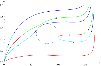
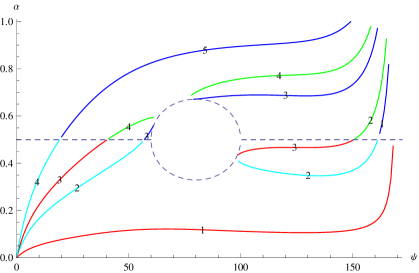
   (a)	(b)

   Figure 7: Plots $\alpha_{n}(\psi)$ for (a) $\theta_{1}=10^{o}$, $\theta_{2}=70^{o}$, $d=6.45$ and (b) $\theta_{1}=10^{o}$, $\theta_{2}=70^{o}$, $d=6.7$.

10. Every trajectory of the types ${}^{-}_{n}\Gamma^{-}_{n+1}$, ${}^{+}_{n}\Gamma^{+}_{n+1}$, ${}^{-}_{n}\Gamma^{+}_{n+1}$ and ${}^{+}_{n-1}\Gamma^{-}_{n}$ is necessary smooth at $\alpha=1/2$ (see section 4.1).

11. Every trajectory of the types ${}^{-}_{n}\Gamma^{-}_{n+1}$ and ${}^{+}_{n}\Gamma^{+}_{n+1}$ is necessary tangent to ${\cal B}_{d}\cup{\cal B}_{u}$ (see section 4.2).

12. The changes of indices in ${\sf Und}_{n_{i}}^{s}$ occur at balloon ${\mathbb{B}}$ in accordance with Table 2 (see Figure 7).

    1. The change of the upper indices ($s\leftrightarrow-s$) and lower indices ($n_{1}\leftrightarrow n_{2}$) occurs at the point $T\in{\cal B}_{l}\cup{\cal B}_{r}$.

    2. The change of the lower index ($n_{1}\leftrightarrow n_{2}$) only occurs at the point $T\in{\cal B}_{d}\cup{\cal B}_{u}$.

       In the nondegenerate case one has $|n_{1}-n_{2}|=1$.

Table 2

$$\begin{array}[]{|c||c|c|c|c|c|c|c|c|c|c|c|}\hline\cr&{}^{-}_{n}\Gamma^{-}_{n+1}&{}^{-}_{n}\Gamma^{+}_{n+1}&{}^{+}_{n-1}\Gamma^{-}_{n}&{}^{+}_{n-1}\Gamma^{+}_{n}\\ \hline\cr\hline\cr{\cal B}_{l}&{}_{n}^{-}T_{n+1}^{+},\quad_{n+1}^{-}T_{n+2}^{+}&{}_{n}^{-}T_{n+1}^{+}&-&{}_{n-1}^{-}T_{n}^{+}\\ \hline\cr{\cal B}_{r}&-&-&{}_{n-1}^{+}T_{n}^{-}&{}_{n-1}^{+}T_{n}^{-},\quad_{n}^{+}T_{n+1}^{-}\\ \hline\cr{\cal B}_{d}&{}_{n}^{-}T_{n+1}^{-}&-&{}_{n-1}^{-}T_{n}^{-}&{}_{n}^{-}T_{n+1}^{-}\\ \hline\cr{\cal B}_{u}&{}_{n+1}^{+}T_{n+2}^{+}&{}_{n+1}^{+}T_{n+2}^{+}&-&{}_{n-1}^{+}T_{n}^{+}\\ \hline\cr\end{array}$$

In Table 2 a symbol ${}^{-}_{n_{1}}T^{+}_{n_{2}}$ denotes a point belonging to two parts ${\sf Und}_{n_{1}}^{-}$ and ${\sf Und}^{+}_{n_{2}}$ of trajectory. Empty boxes mean that corresponding transitions do not exist. The trajectories can be tangent to balloon ${\cal B}_{d}\cup{\cal B}_{u}$ at its left and right points (see Figure 8),

$${}^{-}_{1}T^{+}_{1},\quad^{-}_{2n}T^{+}_{2n+2}\in\;{\cal B}_{l}\cap\left\{{\cal B}_{d}\cup{\cal B}_{u}\right\},\quad\mbox{and}\quad^{-}_{2n}T^{+}_{2n}\in\;{\cal B}_{r}\cap\left\{{\cal B}_{d}\cup{\cal B}_{u}\right\}\;.$$ (5.8)

When $\theta_{2}=\pi/2$ the allowed transitions are the following (see Figure 9),

$${}^{-}_{2n}T^{+}_{2n},\quad^{-}_{2n+1}T^{+}_{2n+1}\in\;{\cal B}_{r}\cap{\cal B}_{l}\;.$$ (5.9)

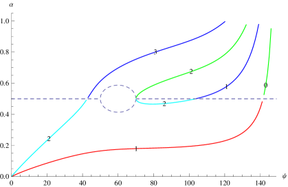
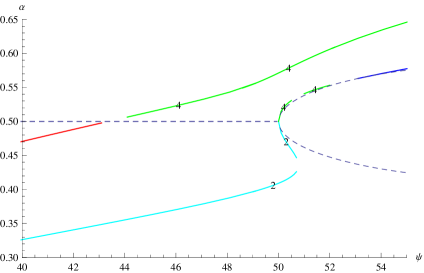
(a)	(b)

Figure 8: Plots $\alpha_{n}(\psi)$ for $\theta_{1}=30^{o}$, $\theta_{2}=80^{o}$ and (a) $d=5.2919$, (b) $d=6.6482$.

6 Saddle Points

For given values of the contact angles $\theta_{1},\theta_{2}$ a change in the distance $d$ value leads to changes of the trajectories shape in $\{\psi,\alpha\}$ plane. Sometimes such transitions are accompanied by drastic changes of the trajectories’ topology characterized by an appearance of the saddle points. The saddle point can be defined as a point that belongs to two trajectories simultaneously.

It is instructive to find the coordinates of the saddle point $\{\psi_{n}^{c},\alpha_{n}^{c}\}$ as well as the distance $d_{n}^{c}$ at which the saddle point is observed. Below we describe a procedure for such computation for each type of the saddle points belonging to a single meniscus type ${\sf Und_{n}^{s}}$.

6.1 Saddle Points of Simple Type

First note that the saddle point may be observed at the intersection of two segments of the curve $\alpha_{n}(\psi)$ determined by the sign $s$ and order $n$ of unduloid meniscus ${\sf Und_{n}^{s}}$ that completely defined by the relation (4.2). At every point of these segments (except the saddle point) one can define the derivative $\alpha_{n}^{\prime}(\psi)$ having a unique value determined from the equation (4.3) where both $A_{n}^{s}$ and $B_{n}^{s}$ do not vanish simultaneously. At the saddle point the derivative $\alpha_{n}^{\prime}(\psi)$ is not unique and in this case $A_{n}^{s}=B_{n}^{s}=0$. Thus the saddle point $\{\psi_{n}^{c},\alpha_{n}^{c}\}$ at $d=d_{n}^{c}$ is determined from the condition $A_{n}^{s}=B_{n}^{s}=0$ together with (4.2).

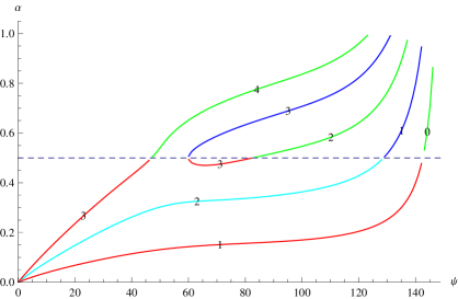
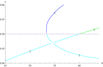
(a)	(b)

Figure 9: Plots $\alpha_{n}(\psi)$ for $\theta_{1}=30^{o}$, $\theta_{2}=90^{o}$ at (a) $d=7.66209$ and (b) $d=5.82697$. In (b) a vicinity of the saddle point ${\sf B_{2}^{-}}$ is shown.

Using the condition $A_{n}^{s}=0$ we find the expression in the square brackets in (4.4) and substituting it into (4.5) we obtain at the saddle point

$$B_{n}^{s}=2\alpha_{n}\Psi\frac{\sin\theta_{1}}{\sin\psi}-\frac{4\alpha_{n}(1-\alpha_{n})}{2\alpha_{n}-1}\Psi\cos t_{1}-\frac{4\alpha_{n}^{2}-2\alpha_{n}-1}{2\alpha_{n}-1}\sin t_{1}\sin\psi+\sin^{2}\psi.$$ (6.1)

Use (6.1) in the condition $B_{n}^{s}=0$ to express $\Psi$ at the saddle point

$$\Psi_{n}^{c}=\frac{\sin^{2}\psi\left[\left(4\alpha_{n}^{2}-2\alpha_{n}-1\right)\sin t_{1}-(2\alpha_{n}-1)\sin\psi\right]}{2\alpha_{n}\left[(2\alpha_{n}-1)\sin\theta_{1}-2(1-\alpha_{n})\cos t_{1}\sin\psi\right]},$$ (6.2)

and eliminate

$$d_{n}^{c}=\Psi_{n}^{c}+\cos\psi_{n}^{c}-1,$$ (6.3)

from the saddle point conditions. Thus we arrive at the final equations determining the saddle point position in the $\{\psi,\alpha\}$ plane:

$$2\alpha_{n}\Psi_{n}^{c}\sin t_{1}-\left[I_{1}(t_{1},t_{2})+sI_{2}(t_{1},t_{2})+n\hat{I}_{2}-s(1-\cos\pi n)I_{2}(\pi/2,t_{2})\right]\sin\psi = 0,$$ (6.4)

$$\Psi_{n}^{c}+(2\alpha_{n}-1)\sin t_{1}\sin\psi\left[sI_{4}(t_{1},t_{2})-2n\hat{I}_{2}^{\prime}(c)-s(1-\cos\pi n)I_{4}(\pi/2,t_{2})\right] = 0.$$ (6.5)

Solving the equations (6.4,6.5) we find the saddle point. An example of trajectories in a vicinity of such a point is shown in Figure 10(a).

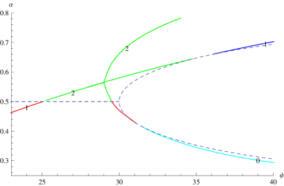
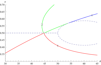
(a)	(b)

Figure 10: The saddle points at intersection of ${}^{-}_{n}\Gamma^{+}_{n}$ and ${}^{+}_{n-1}\Gamma^{+}_{n+1}$ trajectories for $n=1$. (a) The trajectories in the vicinity of ${\sf B_{2}^{+}}$ saddle point for $\theta_{1}=30^{o},\theta_{2}=60^{o}$ and $d=1.05187$. (b) The trajectories in the vicinity of ${\sf B_{1}^{0}}$ mixed type saddle point observed for $\theta_{1}=30^{o},\theta_{2}=80^{o}$ and $d=2.2465$. Colors and numbers correspond to indices of respective unduloids.

6.2 Saddle Points of Mixed Types

The saddle points considered above belong to a single type of unduloid meniscus and are characterized, in particular, by the sign of $\alpha_{n}-1/2$. When at the saddle point $\alpha_{n}=1/2$ this point belongs to two different types of menisci of different orders and signs. These points do not have unduloid sign characteristics and we designate them by a smaller (of two) order only. Consider first such saddle points located to the left of the balloon ($\Theta_{min},\Theta_{max}>0$). This transition described in Section 4.1 happens when $t_{1}=t_{\ast}^{+}=\arcsin\sqrt{-c}$. Equation (6.5) cannot be used directly at $\alpha_{n}=1/2$ as integral $I_{4}$ diverges at $t_{1}=t_{\ast}^{+}$. In the limit $\alpha\to 1/2$ we have by (2.24),

$$I_{4}(t_{\ast}^{+},t_{2})\sim-\frac{1}{|1-2\alpha|\sqrt{1+c}}$$

and obtain from (6.5)

$$\Psi_{\ast}=\sin\psi\tan t_{\ast}^{+}.$$ (6.6)

Note that this value does not depend on both order $n$ and contact angle $\theta_{2}$. Substitution of (6.6) into (6.4) produces a condition on $c$ value

$$I_{1}(t_{\ast}^{+},t_{2})-I_{2}(t_{\ast}^{+},t_{2})+n\hat{I}_{2}+(1-\cos\pi n)I_{2}(\pi/2,t_{2})+\frac{c}{\sqrt{1+c}}=0,$$ (6.7)

where order $n$ corresponds to the meniscus with $\alpha_{n}<1/2$. For given values of order $n$ and contact angle $\theta_{2}$ we find $c$ value verifying the last condition that leads to determination of $\psi_{\ast}=\arcsin\sqrt{-c}-\theta_{1}$. Using it in (6.6) and (6.3) we arrive at the distance $d_{\ast}$ value for which the mixed saddle point is observed. An example of such a point is shown in Figure 10(b).

Consider a mixed type saddle points located to the right of the balloon. This transition described in (4.1) happens for $s=-1$ when $t_{1}=t_{\ast}^{-}=\pi-\arcsin\sqrt{-c}$. Equation (6.5) leads to

$$\Psi_{\ast}=\sin\psi\tan t_{\ast}^{-}.$$

Using it in (6.4) we obtain a condition on $c$ value

$$I_{1}(t_{\ast}^{-},t_{2})-I_{2}(t_{\ast}^{-},t_{2})+n\hat{I}_{2}+(1-\cos\pi n)I_{2}(\pi/2,t_{2})-\frac{c}{\sqrt{1+c}}=0,$$ (6.8)

where positive order $n$ corresponds to the meniscus with $\alpha_{n}<1/2$. Show that the equation (6.8) does not have solutions for $n>0$. Using the relation

$$I_{2}(t_{\ast}^{-},t_{2})=\frac{\hat{I}_{2}}{2}+I_{2}(\pi/2,t_{2}),$$

rewrite the left hand side of (6.8) as

$$\frac{1}{\sqrt{1+c}}+\cos t_{2}+(n-1/2)\hat{I}_{2}-\cos\pi nI_{2}(\pi/2,t_{2}),$$

where sum $s_{1}$ of the first two terms is always positive. For odd $n=2k-1$ we have $s_{1}+(2k-1/2)\hat{I}_{2}+I_{2}(\pi/2,t_{2})>0.$ For even $n=2k$ we have $s_{1}+(2k-1/2)\hat{I}_{2}-I_{2}(\pi/2,t_{2})>0,$ as $I_{2}(\pi/2,t_{2})\leq I_{2}(\pi/2,t_{\ast}^{\pm})=\hat{I}_{2}/2$. Thus the saddle points of the mixed type cannot be observed to the right of the balloon.

6.3 Saddle Points Sequences

The computation of the saddle point position for fixed values of the contact angles $\theta_{1},\theta_{2}$ and increasing $n$ shows that for large $n$ a sequence $\{\psi_{n}^{c},\alpha_{n}^{c}\}$ accumulates in a small vicinity of a point $\{\psi_{\ast}^{c},\alpha_{\ast}^{c}\}$ belonging to the balloon (not reaching it), i.e., $\alpha_{\ast}^{c}=\beta^{s}(\psi_{\ast}^{c})$ as shown in Figure 11.

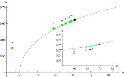
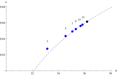
(a)	(b)
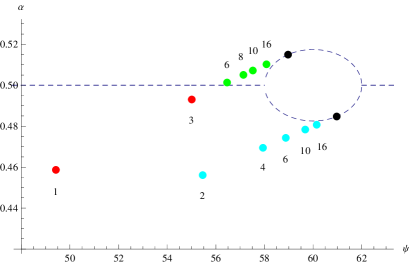
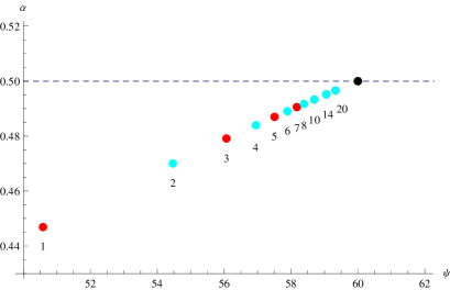
(c)	(d)

Figure 11: (a) The saddle points (green) ${\sf B_{2}^{+}}$ and ${\sf A_{2k}^{+}}$ for $\theta_{1}=30^{o},\theta_{2}=60^{o}$ and $k=2,3,4,7,10$ approach the accumulation point (black) on the balloon with growth of the index $2k$ marking the saddle points. The inset shows saddle points (cyan) ${\sf A_{2k}^{-}}$ for $k=1,2,3,4,7,10$ approaching the accumulation point. (b) The saddle points (blue) ${\sf A_{2k-1}^{+}}$ for $\theta_{1}=30^{o},\theta_{2}=120^{o}$ and $k=2,3,4,5,8,11$ approach the accumulation point (black). (c) For $\theta_{1}=30^{o},\theta_{2}=88^{o}$ the saddle points ${\sf B_{n}^{-}}$ for $n=1,3$ (red), $n=2,4,6,10,16$ (cyan) and ${\sf B_{n}^{+}}$ (green) for $n=6,8,10,16$ approach the corresponding accumulation points (black). (d) For $\theta_{1}=30^{o},\theta_{2}=90^{o}$ the saddle points ${\sf B_{n}^{-}}$ for $n=1,3,5,7$ (red) and $n=2,4,6,8,10,14,20$ (cyan) approach the accumulation point (black).

It is instructive to determine the position of the accumulation point $\{\psi_{\ast}^{c},\alpha_{\ast}^{c}\}$. First note that in (6.4) for $n\gg 1$ the dependence of $\Psi_{n}^{c}$ on $n$ is determined by a relation

$$2\alpha_{n}^{c}\Psi_{n}^{c}\sin t_{1}=n\hat{I}_{2},$$

implying that both $\Psi_{n}^{c}$ and $d_{n}^{c}$ grow linearly in $n$. As the integral $\hat{I}_{2}^{\prime}(c)$ is always negative for $c<0$ then the leading term for $n\gg 1$ in (6.5) is contributed by the integrals $I_{4}$. From (2.24) it follows that the proper divergence is provided by the term $\sin 2t_{2}/[2(1+c)\sqrt{\sin^{2}t_{2}+c}]$ when $c\to-\sin^{2}t_{2}$. Substitution of $\beta^{s}(\psi)$ in (2.9) shows that $c+\sin^{2}\theta_{2}=0$ holds on the balloon. Thus the divergence of $\Psi_{n}^{c}$ used in (6.2) leads to the condition

$$(2\alpha_{\ast}^{c}-1)\sin\theta_{1}=2(1-\alpha_{\ast}^{c})\sin\psi_{\ast}^{c}\cos(\theta_{1}+\psi_{\ast}^{c}),$$ (6.9)

where

$$\alpha_{\ast}^{c}=\frac{1}{2}\left(1+s\sqrt{1-\frac{\sin^{2}\theta_{2}}{\sin^{2}(\theta_{1}+\psi_{\ast}^{c})}}\;\right)=\beta^{s}(\psi_{\ast}^{c}).$$

It follows from (6.9) that the accumulation point with $\alpha_{\ast}^{c}<1/2$ can be observed for $\psi_{\ast}^{c}>\pi/2-\theta_{1}$, while at the point with $\alpha_{\ast}^{c}>1/2$ we have $\psi_{\ast}^{c}<\pi/2-\theta_{1}$. The relation (6.9) also implies

$$2(1-\alpha_{\ast}^{c})\sin(\theta_{1}+\psi_{\ast}^{c})\cos\psi_{\ast}^{c}=\sin\theta_{1},\ \ \ 2\alpha_{\ast}^{c}\sin(\theta_{1}+\psi_{\ast}^{c})\cos\psi_{\ast}^{c}=\sin(\theta_{1}+2\psi_{\ast}^{c}).$$

Multiplying these relations and using the definition (2.9) we find the sign independent condition on the accumulation point

$$\sin\theta_{1}\sin(\theta_{1}+2\psi_{\ast}^{c})=\sin^{2}\theta_{2}\cos^{2}\psi_{\ast}^{c}.$$ (6.10)

It can be shown that the equation (6.10) has two solutions $\psi_{\ast}^{c}$ corresponding to the accumulation points belonging to $\beta^{s}(\psi)$. Computing $\psi_{\ast}^{c}$ from (6.9) or (6.10) we find a growth rate of $d_{n}^{c}$ for large $n$ which is given by

$$\frac{\sin\psi_{\ast}^{c}}{2\alpha_{\ast}^{c}\sin\left(\theta_{1}+\psi_{\ast}^{c}\right)}\hat{I}_{2}\left(-\sin^{2}\theta_{2}\right)=\frac{\sin 2\psi_{\ast}^{c}}{2\sin\left(\theta_{1}+2\psi_{\ast}^{c}\right)}\hat{I}_{2}\left(-\sin^{2}\theta_{2}\right).$$

7 Touching and Intersecting Bodies

When the distance $d$ between the solids is non-positive it leads to strong simplification of the topological structure of the solutions of (2.1). First, only a single branch of the solution that always includes ${\sf Nod^{+}}$ meniscus survives. It follows from the statement made in section 3.4 that spheres ${\sf Sph^{+}_{n}}$, $n>0$, cannot exist when $d\leq 0$, so that only the trajectory that contains ${\sf Sph^{+}_{0}}$ can be observed in $\{\psi,\alpha\}$ plane.

For $d=0$ (the solid sphere on the plane) we show in Appendix C.2 that the curvature of the ${\sf Nod^{-}}$ is negative and diverges as $H\sim\psi^{-2}$ as $\psi\to 0$, confirming the result reported in [5]. In case $\theta_{1}+\theta_{1}>\pi$ one can observe similar divergence of positive curvature for ${\sf Nod^{+}}$ at small $\psi$. The same ${\sf Nod^{+}}$ meniscus can be found in special case $\theta_{1}+\theta_{1}=\pi$ when the curvature diverges as $H\sim\psi^{-1}$. In two last cases the whole trajectory is represented by ${\sf Nod^{+}}$ meniscus (see Figure 3(b)).

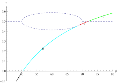
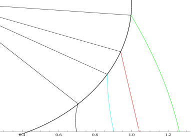
(a)	(b)

Figure 12: (a) Plot $\alpha(\psi)$ for $\theta_{1}=30^{o}$, $\theta_{2}=80^{o}$ and $d=-0.1$, i.e., $\psi_{*}=25.84^{o}$, and (b) four menisci ${\sf Nod^{-}}$ (black), ${\sf Und^{-}_{0}}$ (cyan), ${\sf Und^{-}_{1}}$ (red) and ${\sf Und^{+}_{0}}$ (green) for $\psi=45^{o}$, $\psi=60^{o}$, $\psi=70^{o}$ and $\psi=85^{o}$, respectively.

Another divergent behavior of the curvature is observed when $d<0$ (the solid sphere intersecting the plane). In this case the menisci can exist only for $\psi\geq\psi_{\ast}=\arccos(1+d)$. Formula (C.27) shows that the curvature diverges as $H\sim(\psi-\psi_{\ast})^{-1}$ as $\psi\to\psi_{\ast}$. Depending on the parameters values this divergence is observed for menisci,

$${\sf Nod^{-}}:\quad H<0,\;\;\theta_{1}+\theta_{1}+\psi_{\ast}<\pi,\quad\mbox{and}\quad{\sf Nod^{+}}:\quad H>0,\;\;\theta_{1}+\theta_{1}+\psi_{\ast}>\pi.$$ (7.1)

When $\theta_{1}+\theta_{1}+\psi_{\ast}=\pi$ we show in C.2 that the ${\sf Nod^{-}}$ meniscus is forbidden while the ${\sf Nod^{+}}$ meniscus is observed in the whole range $\psi>\psi_{\ast}$ and its curvature does not diverge. In Figure 12 the $\alpha(\psi)$ trajectory for contact angles $\theta_{1}=30^{o}$, $\theta_{2}=80^{o}$ and $d=-0.1$ is drawn. We present also the four different menisci observed in this case.

The case of intersecting bodies $d<0$ does not lead to change of formula (2.10) for meniscus curvature $H$ and (2.11) for surface area $S$. However formula for the volume $V_{-}(d)$ of meniscus with $d<0$ reads

$$V_{-}(d)=\frac{\pi}{8H^{3}}J_{s}-\frac{\pi}{3}\left(2-3\cos\psi+\cos^{3}\psi\right)+\frac{\pi d^{2}}{3}(3+d),\quad d<0,$$ (7.2)

where integral $J_{s}$ is given in (2.12).

8 Concluding Remarks and Open Problems

Extending the rigorous approach used [5] to describe the menisci shapes between two touching ($d=0$) axisymmetric solids, sphere and plane, we develop a theory of pendular rings in its general form for the separated ($d>0$) or intersecting ($d<0$) solids. The main results are listed below.

1. The YL equation (2.1) with boundary conditions can be viewed as a nonlinear eigenvalue problem. Its unduloidal solutions exhibit a discrete spectrum and are enumerated by two indices: the number $n\in{\mathbb{Z}}_{+}\cup\{0\}$ of inflection points on the meniscus meridional profile ${\cal M}$ and the index $s=\mbox{sgn}(2\alpha_{n}-1)$ determined by the shape of a segment of the curve ${\cal M}$ touching the solid sphere: the shape is either convex, $s=1$, or concave, $s=-1$.

   Menisci shapes $z_{n}^{s}(r)$ and their curvatures $H_{n}^{s}$ play a role of eigenfunctions and eigenvalues of equation (2.1), respectively. The Neeman boundary conditions, two contact angles $\theta_{1}$ and $\theta_{2}$, and a single governing parameter $d>-2$ together with one more parameter, the filling angle $\psi$, completely determine the meniscus shape $z_{n}^{s}(r)$ and curvature evolution $H=H_{n}^{s}(\psi)$.

2. For the fixed $\theta_{1}$ and $\theta_{2}$ the set of the functions $H_{n}^{s}(\psi)$ behaves in such a way that in the plane $\{\psi,H\}$ there exists a bounded domain ${\mathbb{B}}$ where $H_{n}^{s}(\psi)$ do not exist for any $d$.

   Under non-linear transformation $\alpha_{n}(\psi)=H_{n}^{s}(\psi)\sin\psi/\sin(\theta_{1}+\psi)$ this domain ${\mathbb{B}}$ in the plane $\{\psi,\alpha\}$ takes a simple shape with a smooth boundary $\beta^{\pm}(\psi)$ which we call a balloon. At this boundary and at the line $\alpha=1/2$ there occur all transitions between different types of unduloidal menisci. The other two lines $\alpha=0,1$ are also the locations of special menisci: all spherical menisci ${\sf Sph^{+}_{n}}$ at $\alpha=1$, all spherical menisci ${\sf Sph^{-}_{n}}$ at $\alpha=0$ and also catenoidal menisci ${\sf Cat}$ at $\alpha=0$.

   A behavior of $\alpha_{n}(\psi)$ curves reminds in some cases the 2-dim dynamical system with trajectories ramified in a non-simply connected domain $\Delta^{\prime}$. This global representation allows to classify possible trajectories and introduce a saddle point notion into the PR problem. We observe several types of saddle points and give their classification.

3. If the distance between the solids is non-positive, $d\leq 0$, then a single (possibly disconnected) sequence of solutions (menisci), that always includes the ${\sf Nod^{+}}$ type, survives. We describe the asymptotic behavior of the mean curvature $H_{0}^{-}(\psi)$ of nodoidal meniscus in vicinity of a singular point $\psi_{*}=\arccos(1+d)$; such singular point does not exist for $d>0$.

Beyond the scope of the present paper we have left several questions which are related to the theory developed here. Below we mention two of them.

1. The theory of pendular rings in the special cases of boundary conditions:

   • $\theta_{1}=0$, this implies $\alpha=H$ and asymptotics (C.24) of the ${\sf Nod^{+}}$ meniscus curvature fails. This is the case of completely wetted sphere.

   • $\theta_{2}=\pi/2$, the balloon ${\mathbb{B}}$ is reduced to a line $\alpha=1/2$ with one singular point $\psi=\pi/2-\theta_{1}$. This is the case of two solid spheres of equal radii.

   • $\theta_{1}=\theta_{2}$, the balloon ${\mathbb{B}}$ is located in region $0\leq\psi\leq\pi-2\theta_{1}$ and the domain $\Delta^{\prime}$ becomes simply connected. This is the case of two solids of the same material.

   • $\theta_{1}+\theta_{2}=\pi$, $\theta_{2}>\theta_{1}$, the balloon ${\mathbb{B}}$ is located in region $0\leq\psi\leq\theta_{2}-\theta_{1}$ and the domain $\Delta^{\prime}$ becomes simply connected. The physical meaning of this case is unclear.

2. Stability of pendular rings. In this regard, we know only two papers where the stability was studied for the ${\sf Nod^{+}}$ and ${\sf Und_{0}^{+}}$ menisci [8] and those menisci which occur as volume decreases from a convex bridge [9] between two solid spheres of equal radii. The rest of meniscus types including those with inflection points are open for analysis.

Appendices

Appendix A Menisci Formulae

A.1 Catenoids ${\sf Cat}$

The catenoid case is the simplest one that requires a solution of the equation (2.2) with $H=0$. This shape corresponds to the transition from the concave nodoid to concave unduloid. The solution for positive $x$ and $C$ reads $x=C/\sin t$. Using the boundary condition we find

$$C=\sin t_{1}\sin\psi\;.$$ (A.1)

Employing (2.4) we obtain the vertical component of the catenoid meridional profile

$$y=\int_{t_{2}}^{t}\tan t\;dx=-C\int_{t_{2}}^{t}\frac{dt}{\sin t}=C\left(\ln\cot\frac{t}{2}-\ln\cot\frac{t_{2}}{2}\right)\;.$$ (A.2)

Using the boundary condition (2.3) we find a relation

$$1+d-\cos\psi=\sin t_{1}\sin\psi\left(\ln\cot\frac{t_{1}}{2}-\ln\cot\frac{t_{2}}{2}\right)=\sin t_{1}\sin\psi\;\ln\frac{\sin t_{2}(1+\cos t_{1})}{\sin t_{1}(1+\cos t_{2})}\;,$$ (A.3)

that implicitly defines the value of the filling angle $\psi$ at which catenoid is found. The last condition can be rewritten in the form

$$\tan\frac{t_{1}}{2}\cot\frac{t_{2}}{2}=\exp\left(-\frac{1+d-\cos\psi}{\sin\psi\sin t_{1}}\right)\;.$$ (A.4)

Shape of catenoid is found in parametric form

$$x(t)=\frac{C}{\sin t}\;,\quad y(t)=C\left(\ln\cot\frac{t}{2}-\ln\cot\frac{t_{2}}{2}\right)\;.$$ (A.5)

The solid of rotation volume is given by the formula (2.12) with $x=C/\sin t$. From (2.4) we find $dy=-Cdt/\sin t$, so that the ring volume reads

$$-\pi C^{3}\int_{t_{2}}^{t_{1}}\frac{dt}{\sin^{3}t}=\frac{\pi C^{3}}{2}\left(\frac{\cos t_{1}}{\sin^{2}t_{1}}-\frac{\cos t_{2}}{\sin^{2}t_{2}}+\ln\cot\frac{t_{1}}{2}-\ln\cot\frac{t_{2}}{2}\right).$$

The volume of the ${\sf Cat}$ meniscus reads

$$V=\frac{\pi C^{3}}{2}\left(\frac{\cos t_{1}}{\sin^{2}t_{1}}-\frac{\cos t_{2}}{\sin^{2}t_{2}}+\ln\cot\frac{t_{1}}{2}-\ln\cot\frac{t_{2}}{2}\right)-\frac{\pi}{3}(2-3\cos\psi+\cos^{3}\psi)\;.$$ (A.6)

The surface area of the ${\sf Cat}$ meniscus is given by (2.11) with $x=C/\sin t$ producing

$$S=-2\pi C^{2}\int_{t_{2}}^{t_{1}}\frac{dt}{\sin^{3}t}=\pi C^{2}\left(\frac{\cos t_{1}}{\sin^{2}t_{1}}-\frac{\cos t_{2}}{\sin^{2}t_{2}}+\ln\cot\frac{t_{1}}{2}-\ln\cot\frac{t_{2}}{2}\right)\;.$$ (A.7)

A.2 Nodoids ${\sf Nod^{\pm}}$

The curvature expression reads

$$2H\Psi=I_{1}(t_{1},t_{2})+sI_{2}(t_{1},t_{2})\;.$$ (A.8)

The meniscus nodoid shape is given by

$$x(t)=\frac{1}{2H}\left(\sin t+s\sqrt{\sin^{2}t+c}\right)\;,\quad y(t)=\frac{1}{2H}\left[I_{1}(t,t_{2})+sI_{2}(t,t_{2})\right]\;.$$ (A.9)

Using the formulas (2.12) and (2.22) we have for the nodoid volume

$$V=\frac{\pi}{8H^{3}}\left[4J_{3}(t_{1},t_{2})+cI_{1}(t_{1},t_{2})-scI_{2}(t_{1},t_{2})+4sJ_{2}(t_{1},t_{2})\right]-\frac{\pi}{3}(2-3\cos\psi+\cos^{3}\psi)\;.$$ (A.10)

Using the formulas (2.11) and (2.19) we find the nodoid surface area

$$S=\frac{\pi}{2H^{2}}K_{s}(t_{1},t_{2})\;.$$ (A.11)

A.3 Unduloids ${\sf Und_{0}^{\pm}}$

The curvature expression reads

$$2H_{0}^{s}\Psi=I_{1}(t_{1},t_{2})+sI_{2}(t_{1},t_{2})\;.$$ (A.12)

The meniscus unduloid shape is given by (2.5) as

$$x(t)=\frac{1}{2H_{0}^{s}}\left(\sin t+s\sqrt{\sin^{2}t+c}\;\right)\;,\quad y(t)=\frac{1}{2H_{0}^{s}}\left[I_{1}(t,t_{2})+sI_{2}(t,t_{2})\right]\;.$$ (A.13)

Using the formulae (2.12) and (2.22) we have for the unduloid volume

$$V_{0}^{s}=\frac{\pi}{8(H_{0}^{s})^{3}}\left[4J_{3}(t_{1},t_{2})+cI_{1}(t_{1},t_{2})-scI_{2}(t_{1},t_{2})+4sJ_{2}(t_{1},t_{2})\right]-\frac{\pi}{3}(2-3\cos\psi+\cos^{3}\psi)\;.$$ (A.14)

Using the formulae (2.11) and (2.19) we have for the unduloid surface area

$$S_{0}^{s}=\frac{\pi}{2(H_{0}^{s})^{2}}K_{s}(t_{1},t_{2})\;.$$ (A.15)

A.4 Inflectional Unduloids ${\sf Und_{1}^{\pm}}$ with Single Inflection Point

The inflection point $u_{\ast}$ of unduloid satisfies a condition $u_{\ast}^{2}+c=0$ for negative $c$. The inflection point at the sphere surface corresponds to

$$H_{n}^{s}=\frac{\sin t_{1}}{2\sin\psi},$$ (A.16)

while when this point is at the plane

$$H_{n}^{s}=\frac{\sin t_{1}+s\sqrt{\sin^{2}t_{1}-\sin^{2}t_{2}}}{2\sin\psi}.$$ (A.17)

Substitution of (A.16, A.17) into (A.12) for given $s$ generates equations for the critical values $\psi_{1}^{\ast}$ and $\psi_{2}^{\ast}$ of the filling angle at which the inflection point is at the sphere and at the plane, respectively. In case $\psi_{1}^{\ast}=\psi_{2}^{\ast}$ inflectional unduloid reduces to the cylinder reached for $t_{2}=\pi/2$ at $t_{1}^{\ast}=\pi/2$ for all $\theta_{1}<\pi/2$. It has curvature equal to $H_{1}^{s}=(2\cos\theta_{1})^{-1}$.

The integrals in (2.6) and (2.10) in case of inflectional unduloid should be broken into two integrals. The meridional profile is made of two unduloid profiles matching at the point $\{x_{\ast},y_{\ast}\}$, i.e., $u=u_{\ast}$. Consider the case of the ${\sf Und_{1}^{-}}$ meniscus when the profiles touching the plane and the sphere have positive and negative curvature, respectively. Using (A.13) we write for the convex unduloid part

$$x(t)=\frac{1}{2H_{1}^{-}}\left(\sin t+\sqrt{\sin^{2}t+c}\;\right)\;,\quad y(t)=\frac{1}{2H_{1}^{-}}\left[I_{1}(t,t_{2})+I_{2}(t,t_{2})\right]\;,\quad t\in\{t_{2},t_{\ast}\}\;.$$ (A.18)

The upper concave unduloid part is given by

$$x(t)=\frac{1}{2H_{1}^{-}}\left(\sin t-\sqrt{\sin^{2}t+c}+A_{x}\right),\quad y(t)=\frac{1}{2H_{1}^{-}}\left[I_{1}(t,t_{2})-I_{2}(t,t_{2})+A_{y}\right]\;,\quad t\in\{t_{1},t_{\ast}\}.$$

The values of $A_{x}$ and $A_{y}$ have to be found from the matching conditions at $t=t_{\ast}$. Using $u_{\ast}=\sin t_{\ast}=\sqrt{-c}$ we get $t_{\ast}^{-}=\pi-\arcsin\sqrt{-c}$ and $\cos t_{\ast}^{-}=-\sqrt{1+c}$. At the inflection point we find

$$x_{\ast} = \frac{\sqrt{-c}}{2H_{1}^{-}}=\frac{\sqrt{-c}+A_{x}}{2H_{1}^{-}},$$

$$y_{\ast} = \frac{1}{2H_{1}^{-}}\left[I_{1}(t_{\ast}^{-},t_{2})+I_{2}(t_{\ast}^{-},t_{2})\right]=\frac{1}{2H_{1}^{-}}[I_{1}(t_{\ast}^{-},t_{2})-I_{2}(t_{\ast}^{-},t_{2})+A_{y}].$$ (A.19)

The matching conditions produce $A_{x}=0,\ A_{y}=2I_{2}(t_{\ast}^{-},t_{2}),$ leading to the following shape of upper concave unduloid

$$x(t)=\frac{1}{2H_{1}^{-}}\left(\sin t-\sqrt{\sin^{2}t+c}\right),\quad y(t)=\frac{1}{2H_{1}^{-}}\left[I_{1}(t,t_{2})-I_{2}(t,t_{2})+2I_{2}(t_{\ast}^{-},t_{2})\right].$$ (A.20)

Using the second equation in (A.20) we have for $t=t_{1}$

$$2H_{1}^{-}\Psi=I_{1}(t_{1},t_{2})-I_{2}(t_{1},t_{2})+2I_{2}(t_{\ast}^{-},t_{2}).$$ (A.21)

The case of the ${\sf Und_{1}^{+}}$ meniscus when the profile touching the plate has negative curvature, and the profile touching the sphere has positive curvature is treated similarly and we obtain the general expression for the curvature:

$$2H_{1}^{s}\Psi=I_{1}(t_{1},t_{2})+s\left[I_{2}(t_{1},t_{2})-2I_{2}(t_{\ast}^{s},t_{2})\right].$$ (A.22)

A.4.1 Shape

The meniscus shape is given by the following general expressions:

$$x(t)=\frac{1}{2H_{1}^{s}}\left(\sin t-s\sqrt{\sin^{2}t+c}\right),\;y(t)=\frac{1}{2H_{1}^{s}}\left[I_{1}(t,t_{2})-sI_{2}(t,t_{2})\right],\;t\in\{t_{2},t_{\ast}^{s}\},$$

$$x(t)=\frac{1}{2H_{1}^{s}}\left(\sin t+s\sqrt{\sin^{2}t+c}\right),\ y(t)=\frac{1}{2H_{1}^{s}}\left[I_{1}(t,t_{2})+s(I_{2}(t,t_{2})-2I_{2}(t_{\ast}^{s},t_{2}))\right],\ t\in\{t_{1},t_{\ast}^{s}\}.$$

A.4.2 Volume

As the ${\sf Und_{1}^{-}}$ meniscus is made of two menisci having shape of concave (upper) and convex (lower) unduloids, a solid of rotation volume equals sum of volumes $V_{l}$ and $V_{u}$ of lower and upper parts, respectively,

$$V_{l} = \frac{\pi}{8(H_{1}^{-})^{3}}\left[4J_{3}(t_{\ast}^{-},t_{2})+cI_{1}(t_{\ast}^{-},t_{2})-cI_{2}(t_{\ast}^{-},t_{2})+4J_{2}(t_{\ast}^{-},t_{2})\right],$$

$$V_{u} = \frac{\pi}{8(H_{1}^{-})^{3}}\left[4J_{3}(t_{1},t_{\ast}^{-})+cI_{1}(t_{1},t_{\ast}^{-})+cI_{2}(t_{1},t_{\ast}^{-})-4J_{2}(t_{1},t_{\ast}^{-})\right].$$

Adding up the above expressions we have for the meniscus volume

$$V_{1}^{-} = \frac{\pi}{8(H_{1}^{-})^{3}}\left\{4J_{3}(t_{1},t_{2})+cI_{1}(t_{1},t_{2})-c\left[I_{2}(t_{\ast}^{-},t_{2})-I_{2}(t_{1},t_{\ast}^{-})\right]+4\left[J_{2}(t_{\ast}^{-},t_{2})-J_{2}(t_{1},t_{\ast}^{-})\right]\right\}$$ (A.23)

$$- \frac{\pi}{3}\left(2-3\cos\psi+\cos^{3}\psi\right)\;.$$

The general formula for the volume of inflectional unduloid reads

$$V_{1}^{s} = \frac{\pi}{8(H_{1}^{-})^{3}}\{4J_{3}(t_{1},t_{2})+cI_{1}(t_{1},t_{2})+sc\left[I_{2}(t_{\ast}^{s},t_{2})-I_{2}(t_{1},t_{\ast}^{s})\right]$$ (A.24)

$$- 4s\left[J_{2}(t_{\ast}^{s},t_{2})-J_{2}(t_{1},t_{\ast}^{s})\right]\}-\frac{\pi}{3}\left(2-3\cos\psi+\cos^{3}\psi\right)\;.$$

A.4.3 Surface Area

Apply the same approach to calculation of the surface area of the ${\sf Und_{1}^{-}}$ meniscus. The area $S_{1}^{-}$ equals the sum of the surface areas $S_{l}$ and $S_{u}$ of lower (convex) and upper (concave) parts, respectively,

$$S_{l}=\frac{\pi}{2H^{2}}K_{+}(t_{\ast}^{-},t_{2})\;,\ \ S_{u}=\frac{\pi}{2H^{2}}K_{-}(t_{1},t_{\ast}^{-}).$$

Adding up the above expressions we have for the meniscus surface area

$$S_{1}^{-}=\frac{\pi}{2(H_{1}^{-})^{2}}[K_{+}(t_{\ast}^{-},t_{2})+K_{-}(t_{1},t_{\ast}^{-})],$$ (A.25)

and we find the formula for the inflectional unduloid surface area

$$S_{1}^{s}=\frac{\pi}{2(H_{1}^{s})^{2}}[K_{-s}(t_{\ast}^{s},t_{2})+K_{s}(t_{1},t_{\ast}^{s})].$$ (A.26)

A.5 Inflectional Unduloids ${\sf Und_{2}^{\pm}}$ with Two Inflection Points

In previous section we consider the simplest basic inflectional unduloid structure characterized by a single inflection point. We show that if the inflection point $t_{\ast}^{-}$ originates at the plane the ${\sf Und_{1}^{-}}$ meniscus emerges, while separation of the inflection point $t_{\ast}^{+}$ from the sphere generates the ${\sf Und_{1}^{+}}$ meniscus.

It is shown in section 4 that the value $\alpha=1/2$ is a critical point at which a transition between the ${\sf Und_{1}^{-}}$ and the ${\sf Und_{0}^{+}}$ menisci takes place when $t_{\ast}^{-}=t_{1}$ and the single inflection point reaches the solid sphere. What does happen when $t_{\ast}^{-}=\pi-t_{1}$ and the inflection point is inside the meridional profile of the ${\sf Und_{1}^{-}}$ meniscus? In this case the second inflection point, namely, with $t_{\ast}^{+}=t_{1}$, separates from the sphere and we observe a meniscus ${\sf Und_{2}^{+}}$ having two inflection points $t_{\ast}^{+}$ and $t_{\ast}^{-}$. The profile of such meniscus is made of three unduloid segments – two convex (touching both the sphere and the plane) and a concave one between them.

Consider derivation of the equation for the curvature for this meniscus. Using (A.13) we write for the lower convex unduloid part touching the plane

$$x(t)=\frac{1}{2H_{2}^{+}}\left(\sin t+\sqrt{\sin^{2}t+c}\;\right),\ y(t)=\frac{1}{2H_{2}^{+}}\left[I_{1}(t,t_{2})+I_{2}(t,t_{2})\right],\ t\in\{t_{2},t_{\ast}^{-}\}.$$

The middle concave unduloid part is given by

$$x(t)=\frac{1}{2H_{2}^{+}}\left(\sin t-\sqrt{\sin^{2}t+c}+A_{x1}\;\right),\ y(t)=\frac{1}{2H_{2}^{+}}\left[I_{1}(t,t_{2})-I_{2}(t,t_{2})+A_{y1}\right],\ t\in\{t_{\ast}^{-},t_{\ast}^{+}\}.$$

Finally, for the upper convex unduloid part touching the sphere we write

$$x(t)=\frac{1}{2H_{2}^{+}}\left(\sin t+\sqrt{\sin^{2}t+c}+A_{x2}\;\right),\ y(t)=\frac{1}{2H_{2}^{+}}\left[I_{1}(t,t_{2})+I_{2}(t,t_{2})+A_{y2}\right],\ t\in\{t_{1},t_{\ast}^{+}\}.$$

The values of $A_{xi}$ and $A_{yi}$ have to be found from the matching conditions at $t=t_{\ast}^{\mp}$ producing

$$A_{x1}=A_{x2}=0,\quad A_{y1}=2I_{2}(t_{\ast}^{-},t_{2}),\quad A_{y2}=2I_{2}(t_{\ast}^{-},t_{2})-2I_{2}(t_{\ast}^{+},t_{2})=2I_{2}(t_{\ast}^{-},t_{\ast}^{+}),$$

leading to the following shape of upper convex unduloid

$$x(t)=\frac{1}{2H_{2}^{+}}\left(\sin t+\sqrt{\sin^{2}t+c}\;\right)\;,\ y(t)=\frac{1}{2H_{2}^{+}}\left[I_{1}(t,t_{2})+I_{2}(t,t_{2})+2I_{2}(t_{\ast}^{-},t_{\ast}^{+})\right]\;.$$ (A.27)

Using the second equation in (A.27) we have for $t=t_{1}$

$$2H_{2}^{+}\Psi=I_{1}(t_{1},t_{2})+I_{2}(t_{1},t_{2})+2I_{2}(t_{\ast}^{-},t_{\ast}^{+}).$$ (A.28)

The case of the ${\sf Und_{2}^{-}}$ meniscus when the profiles touching both the plate and the sphere have negative curvature is treated similarly to obtain

$$2H_{2}^{-}\Psi=I_{1}(t_{1},t_{2})-I_{2}(t_{1},t_{2})+2I_{2}(t_{\ast}^{-},t_{\ast}^{+}).$$ (A.29)

Thus, we obtain the general expression for the curvature for the ${\sf Und_{2}^{\pm}}$ menisci

$$2H_{2}^{s}\Psi=I_{1}(t_{1},t_{2})+sI_{2}(t_{1},t_{2})+2I_{2}(t_{\ast}^{-},t_{\ast}^{+}),$$ (A.30)

As shown in D.2 the value $\hat{I}_{2}$ of integral $I_{2}(t_{\ast}^{-},t_{\ast}^{+})$ reads $\hat{I}_{2}=2\sqrt{-c}E(1+1/c)$.

A.5.1 Shape

The meniscus shape is given by the following general expressions:

$$x(t)=\frac{1}{2H_{2}^{s}}\left(\sin t+s\sqrt{\sin^{2}t+c}\;\right),\ y(t)=\frac{1}{2H_{2}^{s}}\left[I_{1}(t,t_{2})+sI_{2}(t,t_{2})\;\right],\ t\in\{t_{2},t_{\ast}^{-s}\},$$ (A.31)

$$x(t)=\frac{1}{2H_{2}^{s}}\left(\sin t-s\sqrt{\sin^{2}t+c}\;\right),\ y(t)=\frac{1}{2H_{2}^{s}}\left[I_{1}(t,t_{2})-s(I_{2}(t,t_{2})-2I_{2}(t_{\ast}^{s},t_{2}))\right],\ t\in\{t_{\ast}^{-},t_{\ast}^{+}\},$$

$$x(t)=\frac{1}{2H_{2}^{s}}\left(\sin t+s\sqrt{\sin^{2}t+c}\;\right),\ y(t)=\frac{1}{2H_{2}^{s}}\left[I_{1}(t,t_{2})+sI_{2}(t,t_{2})+2\hat{I}_{2}\right],\ t\in\{t_{1},t_{\ast}^{s}\}.$$

A.5.2 Volume

Inflectional unduloid ${\sf Und_{2}^{+}}$ meniscus is made of three menisci having shape of concave (middle segment) and convex (upper and lower segments) unduloids; its volume equals the sum of the volumes $V_{l},V_{m}$ and $V_{u}$ of lower, middle and upper parts, respectively:

$$V_{l} = \frac{\pi}{8(H_{2}^{+})^{3}}[4J_{3}(t_{\ast}^{-},t_{2})+cI_{1}(t_{\ast}^{-},t_{2})-cI_{2}(t_{\ast}^{-},t_{2})+4J_{2}(t_{\ast}^{-},t_{2})]\;,$$

$$V_{m} = \frac{\pi}{8(H_{2}^{+})^{3}}[4J_{3}(t_{\ast}^{+},t_{\ast}^{-})+cI_{1}(t_{\ast}^{+},t_{\ast}^{-})+cI_{2}(t_{\ast}^{+},t_{\ast}^{-})-4J_{2}(t_{\ast}^{+},t_{\ast}^{-})]\;,$$

$$V_{u} = \frac{\pi}{8(H_{2}^{+})^{3}}[4J_{3}(t_{1},t_{\ast}^{+})+cI_{1}(t_{1},t_{\ast}^{+})-cI_{2}(t_{1},t_{\ast}^{+})+4J_{2}(t_{1},t_{\ast}^{+})]\;.$$

Adding up the above expressions we have for the meniscus volume

$$V_{2}^{+} = \frac{\pi}{8(H_{2}^{+})^{3}}\{4J_{3}(t_{1},t_{2})+cI_{1}(t_{1},t_{2})-c[I_{2}(t_{\ast}^{-},t_{2})-I_{2}(t_{\ast}^{+},t_{\ast}^{-})+I_{2}(t_{1},t_{\ast}^{+})]$$ (A.32)

$$+ 4[J_{2}(t_{\ast}^{-},t_{2})-J_{2}(t_{\ast}^{+},t_{\ast}^{-})+J_{2}(t_{1},t_{\ast}^{+})]\}-\frac{\pi}{3}(2-3\cos\psi+\cos^{3}\psi)\;.$$

Using the properties of the integrals $I_{2}$ and $J_{2}$ we find:

$$V_{2}^{+} = \frac{\pi}{8(H_{2}^{+})^{3}}\{4J_{3}(t_{1},t_{2})+cI_{1}(t_{1},t_{2})-c[I_{2}(t_{1},t_{2})-2\hat{I}_{2}]$$ (A.33)

$$+ 4[J_{2}(t_{1},t_{2})-2\hat{J}_{2}]\}-\frac{\pi}{3}(2-3\cos\psi+\cos^{3}\psi)\;,$$

where the value $\hat{J}_{2}$ of integral $J_{2}(t_{\ast}^{-},t_{\ast}^{+})$ is computed in (D.14). The general expression for the menisci volume reads

$$V_{2}^{s} = \frac{\pi}{8(H_{2}^{s})^{3}}\{4J_{3}(t_{1},t_{2})+cI_{1}(t_{1},t_{2})-sc[I_{2}(t_{1},t_{2})+2s\hat{I}_{2}]$$ (A.34)

$$+ 4s[J_{2}(t_{1},t_{2})+2s\hat{J}_{2}]\}-\frac{\pi}{3}(2-3\cos\psi+\cos^{3}\psi)\;.$$

A.5.3 Surface Area

Similar approach is applied for calculation of the surface area of the ${\sf Und_{2}^{+}}$ meniscus. The area $S_{2}^{+}$ equals the sum of the surface areas $S_{l}$, $S_{m}$ and $S_{u}$ of lower, middle and upper segments, respectively,

$$S_{l}=\frac{\pi}{2(H_{2}^{+})^{2}}K_{+}(t_{\ast}^{-},t_{2})\;,\ \ S_{m}=\frac{\pi}{2(H_{2}^{+})^{2}}K_{-}(t_{\ast}^{+},t_{\ast}^{-})\;,\ \ S_{u}=\frac{\pi}{2(H_{2}^{+})^{2}}K_{+}(t_{1},t_{\ast}^{+}).$$

Adding up the above expressions we have for the meniscus surface area

$$S_{2}^{+}=\frac{\pi}{2(H_{2}^{+})^{2}}\left[K_{+}(t_{\ast}^{-},t_{2})+K_{-}(t_{\ast}^{+},t_{\ast}^{-})+K_{+}(t_{1},t_{\ast}^{+})\right].$$ (A.35)

We give a general expression for the menisci surface area

$$S_{2}^{s}=\frac{\pi}{2(H_{2}^{s})^{2}}\left[K_{s}(t_{\ast}^{-s},t_{2})-s\hat{K}_{-s}+K_{s}(t_{1},t_{\ast}^{s})\right].$$ (A.36)

A.6 Inflectional Unduloids ${\sf Und_{3}^{\pm}}$ with Three Inflection Points

In A.5 we consider the inflectional unduloid ${\sf Und_{2}^{\pm}}$ with two inflection points for the values of inflection points parameter $0<t_{\ast}^{\pm}<\pi$. There exist also menisci with larger number of inflection points.

Consider first an inflectional meniscus ${\sf Und_{3}^{-}}$ with three inflection points. A natural way to generate it is to consider the ${\sf Und_{2}^{+}}$ unduloid having two inflection points $t_{\ast,0}^{+}=t_{1}$ and $t_{\ast,0}^{-}=\pi-t_{1}$ and allow at $\alpha=1/2$ a third inflection point $t_{\ast,1}^{-}=\pi-t_{1}$ to separate from the sphere. This point appears due to vertical translational periodicity of the meridional profile. The profile of such a meniscus is made of four unduloids – two convex (one of them touches the sphere) and two concave (one touches the plane). In all formulas below we drop additional indices $k$ of $t_{\ast,k}^{\pm}$. Derivation of the curvature equation for this meniscus is similar to the one of ${\sf Und_{1}^{s}}$ and ${\sf Und_{2}^{s}}$,

$$2H_{3}^{-}\Psi=I_{1}(t_{1},t_{2})-I_{2}(t_{1},t_{2})+2\hat{I}_{2}+2I_{2}(t_{\ast}^{-},t_{2}).$$ (A.37)

A dual inflectional meniscus ${\sf Und_{3}^{+}}$ is generated from the ${\sf Und_{2}^{+}}$ unduloid at $\alpha=\beta^{+}$ by separation of a third inflection point $t_{\ast}^{+}=t_{1}$ from the plane:

$$2H_{3}^{+}\Psi=I_{1}(t_{1},t_{2})+I_{2}(t_{1},t_{2})+2\hat{I}_{2}-2I_{2}(t_{\ast}^{+},t_{2}).$$ (A.38)

Merging (A.37,A.38) we arrive at the general formula for the curvature

$$2H_{3}^{s}\Psi=I_{1}(t_{1},t_{2})+sI_{2}(t_{1},t_{2})-2sI_{2}(t_{\ast}^{s},t_{2})+2\hat{I}_{2}.$$ (A.39)

A.6.1 Shape

The shape of the ${\sf Und_{3}^{s}}$ meniscus is given by the following general expressions

$$x(t)=\frac{1}{2H_{3}^{s}}\left(\sin t-s\sqrt{\sin^{2}t+c}\right),\;y(t)=\frac{1}{2H_{3}^{s}}[I_{1}(t,t_{2})-sI_{2}(t,t_{2})],\;t\in\{t_{2},t_{\ast}^{s}\},$$ (A.40)

$$x(t)=\frac{1}{2H_{3}^{s}}\left(\sin t+s\sqrt{\sin^{2}t+c}\right),\;y(t)=\frac{1}{2H_{3}^{s}}[I_{1}(t,t_{2})+sI_{2}(t,t_{2})-2sI_{2}(t_{\ast}^{s},t_{2})],\;t\in\{t_{\ast}^{s},t_{\ast}^{-s}\}.$$

$$x(t)=\frac{1}{2H_{3}^{s}}\left(\sin t-s\sqrt{\sin^{2}t+c}\right),\;y(t)=\frac{1}{2H_{3}^{s}}[I_{1}(t,t_{2})-sI_{2}(t,t_{2})+2\hat{I}_{2}],\;t\in\{t_{\ast}^{-s},t_{\ast}^{s}\},$$ (A.41)

$$x(t) = \frac{1}{2H_{3}^{s}}\left(\sin t+s\sqrt{\sin^{2}t+c}\right),$$

$$y(t) = \frac{1}{2H_{3}^{s}}[I_{1}(t,t_{2})+sI_{2}(t,t_{2})+2\hat{I}_{2}-2sI_{2}(t_{\ast}^{s},t_{2})],t\in\{t_{1},t_{\ast}^{s}\}.$$ (A.42)

A.6.2 Volume

Inflectional unduloid ${\sf Und_{3}^{s}}$ meniscus is made of four menisci having shape of concave and convex unduloids; its volume $V_{3}^{s}$ equals the sum of the volumes of corresponding parts:

$$V_{3}^{s} = \frac{\pi}{8(H_{3}^{s})^{3}}\{4J_{3}(t_{1},t_{2})+cI_{1}(t_{1},t_{2})+sc[I_{2}(t_{1},t_{2})-2s\hat{I}_{2}-2I_{2}(t_{1},t_{\ast}^{s})]$$ (A.43)

$$- 4s[J_{2}(t_{1},t_{2})-2s\hat{J}_{2}-2J_{2}(t_{1},t_{\ast}^{s})]\}-\frac{\pi}{3}(2-3\cos\psi+\cos^{3}\psi).$$

A.6.3 Surface Area

The surface area $S_{3}^{s}$ of the ${\sf Und_{3}^{s}}$ meniscus equals the sum of the surface areas of corresponding segments:

$$S_{3}^{s}=\frac{\pi}{2(H_{3}^{s})^{2}}\left[K_{-s}(t_{\ast}^{s},t_{2})+\hat{K}_{+}-\hat{K}_{-}+K_{s}(t_{1},t_{\ast}^{s})\right].$$ (A.44)

A.7 Inflectional Unduloids ${\sf Und_{2k}^{\pm}}$ with Even Number of Inflection Points

Generalization of the menisci ${\sf Und_{0}^{s}}$ and ${\sf Und_{2}^{s}}$ to arbitrary even number of inflection points is straightforward, and we present here the final formulas for these menisci. Shape of upper unduloid segment touching the sphere for the ${\sf Und_{2k}^{s}}$ meniscus reads

$$x(t)=\frac{1}{2H_{2k}^{s}}\left(\sin t+s\sqrt{\sin^{2}t+c}\right)\;,\quad y(t)=\frac{1}{2H_{2k}^{s}}[I_{1}(t,t_{2})+sI_{2}(t,t_{2})+2k\hat{I}_{2}]\;.$$ (A.45)

Using the second equation in (A.45) we have for $t=t_{1}$

$$2H_{2k}^{s}\Psi=I_{1}(t_{1},t_{2})+sI_{2}(t_{1},t_{2})+2k\hat{I}_{2}.$$ (A.46)

A.7.1 Shape

The meniscus shape is given for $0\leq n\leq k-1$ by the following general expressions :

$$x(t)=\frac{1}{2H_{2k}^{s}}\left(\sin t+s\sqrt{\sin^{2}t+c}\right),\;y(t)=\frac{1}{2H_{2k}^{s}}\left[I_{1}(t,t_{2})+sI_{2}(t,t_{2})+2n\hat{I}_{2}\right],\;t\in\left\{\tilde{t}_{2},t_{\ast}^{-s}\right\},$$ (A.47)

$$x(t) = \frac{1}{2H_{2k}^{s}}\left(\sin t-s\sqrt{\sin^{2}t+c}\right),\ \ t\in\left\{t_{\ast}^{-},t_{\ast}^{+}\right\},$$

$$y(t) = \frac{1}{2H_{2k}^{s}}\left[I_{1}(t,t_{2})-s(I_{2}(t,t_{2})-2I_{2}(t_{\ast}^{\mp},t_{2}))+2n\hat{I}_{2}\right],$$ (A.48)

$$x(t)=\frac{1}{2H_{2k}^{s}}\left(\sin t+s\sqrt{\sin^{2}t+c}\right),\;y(t)=\frac{1}{2H_{2k}^{s}}\left[I_{1}(t,t_{2})+sI_{2}(t,t_{2})+2k\hat{I}_{2}\right],\;t\in\left\{t_{1},t_{\ast}^{s}\right\},$$ (A.49)

where

$$\tilde{t}_{2}=t_{2}\delta_{n0}+t_{\ast}^{s}(1-\delta_{n0}),$$

$\delta_{ij}$ denotes the Kronecker delta.

A.7.2 Volume

Volume of inflectional unduloid ${\sf Und_{2k}^{s}}$ meniscus is computed as

$$V_{2k}^{s} = \frac{\pi}{8(H_{2k}^{s})^{3}}\{4J_{3}(t_{1},t_{2})+cI_{1}(t_{1},t_{2})-sc[I_{2}(t_{1},t_{2})-2ks\hat{I}_{2}]$$ (A.50)

$$+ 4s[J_{2}(t_{1},t_{2})+2ks\hat{J}_{2}]\}-\frac{\pi}{3}(2-3\cos\psi+\cos^{3}\psi)\;,$$

A.7.3 Surface Area

Surface area of the ${\sf Und_{2k}^{s}}$ meniscus reads

$$S_{2k}^{s}=\frac{\pi}{2(H_{2k}^{s})^{2}}\left[K_{s}(t_{\ast}^{-s},t_{2})+k(\hat{K}_{+}-\hat{K}_{-})+K_{s}(t_{1},t_{\ast}^{-s})\right].$$ (A.51)

A.8 Inflectional Unduloids ${\sf Und_{2k+1}^{\pm}}$ with Odd Number of Inflection Points

Generalization of the menisci ${\sf Und_{1}^{s}}$ and ${\sf Und_{3}^{s}}$ to arbitrary odd number of inflection points is straightforward, and we present here the final formulas for these menisci. We find for the curvature of the ${\sf Und_{2k+1}^{s}}$ meniscus

$$2H_{2k+1}^{s}\Psi=I_{1}(t_{1},t_{2})+sI_{2}(t_{1},t_{2})-2sI_{2}(t_{\ast}^{s},t_{2})+2k\hat{I}_{2}.$$ (A.52)

A.8.1 Shape

The shape of the ${\sf Und_{2k+1}^{s}}$ meniscus is given by the following general expressions for $0\leq n\leq k$

$$x(t) = \frac{1}{2H_{2k+1}^{s}}\left(\sin t-s\sqrt{\sin^{2}t+c}\right),\ \ \ t\in\left\{\tilde{t}_{2},t_{\ast}^{s}\right\},$$

$$y(t) = \frac{1}{2H_{2k+1}^{s}}[I_{1}(t,t_{2})-sI_{2}(t,t_{2})+2n\hat{I}_{2}],$$ (A.53)

$$x(t) = \frac{1}{2H_{2k+1}^{s}}\left(\sin t+s\sqrt{\sin^{2}t+c}\right),\ \ \ t\in\left\{\tilde{t}_{1},t_{\ast}^{s}\right\},$$

$$y(t) = \frac{1}{2H_{2k+1}^{s}}\left[I_{1}(t,t_{2})+sI_{2}(t,t_{2})+2n\hat{I}_{2}-2sI_{2}(t_{\ast}^{s},t_{2})\right],$$ (A.54)

where

$$\tilde{t}_{2}=t_{2}\delta_{n0}+t_{\ast}^{-s}(1-\delta_{n0}),\ \ \ \tilde{t}_{1}=t_{1}\delta_{nk}+t_{\ast}^{-s}(1-\delta_{nk}).$$

A.8.2 Volume

Volume of inflectional unduloid ${\sf Und_{2k+1}^{s}}$ meniscus reads

$$V_{2k+1}^{s} = \frac{\pi}{8(H_{2k+1}^{s})^{3}}\{4J_{3}(t_{1},t_{2})+cI_{1}(t_{1},t_{2})+sc[I_{2}(t_{1},t_{2})-2ks\hat{I}_{2}-2I_{2}(t_{1},t_{\ast}^{s})]$$ (A.55)

$$- 4s[J_{2}(t_{1},t_{2})-2ks\hat{J}_{2}-2J_{2}(t_{1},t_{\ast}^{s})]\}-\frac{\pi}{3}(2-3\cos\psi+\cos^{3}\psi)\;.$$

A.8.3 Surface Area

Surface area of inflectional unduloid ${\sf Und_{2k+1}^{s}}$ meniscus is computed as

$$S_{2k+1}^{s}=\frac{\pi}{2(H_{2k+1}^{s})^{2}}\left[K_{-s}(t_{\ast}^{s},t_{2})+k(\hat{K}_{+}-\hat{K}_{-})+K_{s}(t_{1},t_{\ast}^{s})\right].$$ (A.56)

A.9 Unduloid General Formulas

Merging the expressions (A.46, A.52) we write the general expression for the curvature of ${\sf Und_{n}^{s}}$ unduloid

$$2H_{n}^{s}\Psi=I_{1}(t_{1},t_{2})+sI_{2}(t_{1},t_{2})+n\hat{I}_{2}-s\frac{1-\cos\pi n}{2}\left[I_{2}(t_{\ast}^{+},t_{2})+I_{2}(t_{\ast}^{-},t_{2})\right].$$ (A.57)

It can be checked by direct computation that the expression in the square brackets in (A.57) evaluates to $2I_{2}(\pi/2,t_{2})$, and we have

$$2H_{n}^{s}\Psi=I_{1}(t_{1},t_{2})+sI_{2}(t_{1},t_{2})+n\hat{I}_{2}-s(1-\cos\pi n)I_{2}(\pi/2,t_{2}),$$ (A.58)

Replacing in (A.55) $k$ by $(n-1)/2$ we find for the expression in curly brackets

$$4J_{3}(t_{1},t_{2})+cI_{1}(t_{1},t_{2})+scI_{2}(t_{1},t_{2})-nc\hat{I}_{2}+2scI_{2}(\pi/2,t_{1})-4sJ_{2}(t_{1},t_{2})+4n\hat{J}_{2}-8sJ_{2}(\pi/2,t_{1}).$$

Combining it with (A.50) we find

$$V_{n}^{s} = \frac{\pi}{8(H_{n}^{s})^{3}}\{4J_{3}(t_{1},t_{2})+cI_{1}(t_{1},t_{2})+4n\hat{J}_{2}-\sigma(n)[cI_{2}(t_{1},t_{2})-4J_{2}(t_{1},t_{2})]+nc\hat{I}_{2}\cos\pi n$$ (A.59)

$$+ s(1-\cos\pi n)[cI_{2}(\pi/2,t_{1})-4J_{2}(\pi/2,t_{1})]\}-\frac{\pi}{3}(2-3\cos\psi+\cos^{3}\psi)\;,$$

where $\sigma(n)=s\cdot\cos\pi n$. From (A.51) and (A.56) one finds

$$S_{n}^{s}=\frac{\pi}{2(H_{n}^{s})^{2}}\left[K_{\sigma(n)}\left(t_{\ast}^{-\sigma(n)},t_{2}\right)+\lfloor n/2\rfloor(\hat{K}_{+}-\hat{K}_{-})+K_{s}\left(t_{1},t_{\ast}^{-\sigma(n)}\right)\right],$$ (A.60)

where $\lfloor x\rfloor$ denotes the floor function.

Appendix B Spheres ${\sf Sph_{n}^{\pm}}$

In the classical menisci sequence the transition from convex unduloid to convex nodoid takes place through formation of a spherical surface ${\sf Sph^{+}_{0}}$. The inflectional unduloids ${\sf Und_{n}^{+}}$, $n>0$, in the limit $\alpha_{n}\to 1$ transform into the surfaces ${\sf Sph^{+}_{n}}$ made of several spherical segments. The same time the unduloid menisci ${\sf Und_{n}^{-}}$ at small filling angles approach another type of spherical menisci ${\sf Sph^{-}_{n}}$. Below we treat them both as a limiting case of corresponding ${\sf Und_{n}^{\pm}}$ menisci.

B.1 Asymptotic Behavior of ${\sf Und_{n}^{\pm}}$ Menisci in Vicinity of ${\sf Sph_{n}^{\pm}}$

Consider the relation (A.58) and find dependence $H=H(\psi)$ for the ${\sf Und_{n}^{s}}$ meniscus in vicinity of $c=0$ that can be reached for either $\alpha=0$ (for $s=-1,\psi=\phi_{n}^{-}=0$) or $\alpha=1$ (for $s=1,\psi=\phi_{n}^{+}$). Using (2.7) find asymptotic for $c(\psi)$

$$c(\psi)=c^{\prime}(\phi_{n}^{s})(\psi-\phi_{n}^{s})\;,\quad c^{\prime}(\phi_{n}^{s})=4s|2\alpha_{n}-1|\alpha_{n}^{\prime}(\phi_{n}^{s})\sin^{2}(\theta_{1}+\phi_{n}^{s})\;,\quad\mbox{sgn}\;c^{\prime}(\phi_{n}^{s})=s,$$ (B.1)

where $\alpha_{n}^{\prime}(\phi_{n}^{s})>0$.

To find the asymptotics of the general terms $\sqrt{c}\;\overline{E}(t,\sqrt{-1/c})$ and $\sqrt{c}\;\overline{F}(t,\sqrt{-1/c})$ used in (A.21) we make use of asymptotic expansions for the elliptic integrals based on relations found at [10] and obtain for $t\leq\pi$,

$$\sqrt{c}\;\overline{E}(t,\sqrt{-1/c})\stackrel{{\scriptstyle c\to 0}}{{\simeq}}\tilde{E}(t,c)=1-\cos t-\frac{c}{4}\left(\ln\cot^{2}\frac{t}{2}-4\ln 2+\ln|c|-1\right)\;,$$ (B.2)

$$\sqrt{c}\;\overline{F}(t,\sqrt{-1/c})\stackrel{{\scriptstyle c\to 0}}{{\simeq}}\tilde{F}(t,c)=-\frac{c}{2}\left(\ln\cot^{2}\frac{t}{2}-4\ln 2+\ln|c|\right)\;.$$ (B.3)

Using the above expressions we find an approximation

$$I_{2}(t_{1},t_{2})=I_{1}(t_{1},t_{2})-\frac{c}{2}M,\ \ \ M=\ln\left(\tan\frac{t_{1}}{2}\cot\frac{t_{2}}{2}\right).$$ (B.4)

The last relation leads to

$$\hat{I}_{2}=I_{2}(t_{\ast}^{-},t_{\ast}^{+})=2-c\ln 2+\frac{c}{2}\ln(-c),\ \ I_{2}(\pi/2,t_{2})=\cos t_{2}-\frac{c}{2}\ln\left(\cot\frac{t_{2}}{2}\right).$$ (B.5)

Substitution of (B.4, B.5) into (A.58) produces

$$2H_{n}^{s}\Psi(\phi_{n}^{s})=2n-(1+s)\cos(\theta_{1}+\phi_{n}^{s})-(1+s\cos\pi n)\cos\theta_{2}+\frac{cn}{2}\ln(-c).$$ (B.6)

The curvature at the sphere is found as

$$H_{n}^{s}(\phi_{n}^{s})=\frac{2n-(1+s)\cos(\theta_{1}+\phi_{n}^{s})-(1+s\cos\pi n)\cos\theta_{2}}{2\Psi(\phi_{n}^{s})}.$$ (B.7)

It follows from (B.7) that for the ${\sf Sph^{-}_{n}}$ sphere the curvature is independent of $\theta_{1}$ and reads

$$H_{n}^{-}(0)=\frac{2n-(1-\cos\pi n)\cos\theta_{2}}{2d}.$$ (B.8)

For $s=1$ we find a condition on the angle $\phi_{n}^{+}$ at which sphere ${\sf Sph^{+}_{n}}$ is observed

$$2(1+d-\cos\phi_{n}^{+})\sin(\theta_{1}+\phi_{n}^{+})=\sin\phi_{n}^{+}[2n-2\cos(\theta_{1}+\phi_{n}^{+})-(1+\cos\pi n)\cos\theta_{2}],$$

which reduces to

$$2(1+d)\sin(\theta_{1}+\phi_{n}^{+})-2\sin\theta_{1}-\sin\phi_{n}^{+}[2n-(1+\cos\pi n)\cos\theta_{2}]=0,$$ (B.9)

Differentiating the relation (B.6) we obtain in the leading order

$$\frac{dH_{n}^{s}(\psi)}{d\psi}_{|\;\psi=\phi_{n}^{s}}=\frac{nc^{\prime}(\phi_{n}^{s})}{4\Psi(\phi_{n}^{s})}\;\left[-1+\ln(-c)\right]\;.$$ (B.10)

Combining (B.10) with the last formula in (B.1) we find $\mbox{sgn}\left(dH_{n}^{s}/d\psi\right)\!=\!-s$ at $\psi=\phi_{n}^{s}$. General expression for derivative of $\alpha_{n}$ reads

$$\alpha_{n}^{\prime}(\psi)=\frac{dH_{n}^{s}(\psi)}{d\psi}\frac{\sin\psi}{\sin t_{1}}+H_{n}^{s}\frac{\sin\theta_{1}}{\sin^{2}t_{1}}\;.$$ (B.11)

Using it with (B.8) we find

$$\alpha_{n}^{\prime}(0)=\xi^{-}_{n}=\frac{H_{n}^{-}(0)}{\sin\theta_{1}}=\frac{2n-(1-\cos\pi n)\cos\theta_{2}}{2d\sin\theta_{1}},$$ (B.12)

implying that for small $\psi$ the slope $\xi^{-}_{n}$ of $\alpha$ increases with growth of index $n$ and decreases with growth of the distance $d$. Applying (B.2,B.3) to integral (2.16) we find its asymptotics $I_{3}(t_{1},t_{2})=cM$ and obtain

$$K_{s}(t_{1},t_{2})=2(1+s)(\cos t_{2}-\cos t_{1}).$$

Thus the expression in square brackets in the general formula for unduloid surface area (A.60) is independent of $c$ and reads

$$\bar{K}=4n-2(1+s\cos\pi n)\cos\theta_{2}-2(1+s)\cos(\theta_{1}+\phi_{n}^{s})=4H_{n}^{s}(\phi_{n}^{s})\Psi(\phi_{n}^{s}).$$

Thus the surface area reads in the leading logarithmic order

$$S_{n}^{s}=\frac{\pi\bar{K}}{2(H_{n}^{s})^{2}}=\frac{2\pi\Psi(\phi_{n}^{s})}{H_{n}^{s}(\phi_{n}^{s})},$$ (B.13)

and we find that $\mbox{sgn}\;(dS_{n}^{s}(\psi)/d\psi)=s$ at $\psi=\phi_{n}^{s}$. The explicit expression for the surface area of ${\sf Sph^{s}_{n}}$ reads

$$S_{n}^{s}(\phi_{n}^{s})=\frac{4\pi\Psi^{2}(\phi_{n}^{s})}{2n-(1+s)\cos(\theta_{1}+\phi_{n}^{s})-(1+s\cos\pi n)\cos\theta_{2}},$$ (B.14)

and we find for ${\sf Sph^{-}_{n}}$

$$S_{n}^{-}(0)=\frac{4\pi d^{2}}{2n-(1-\cos\pi n)\cos\theta_{2}}\;.$$ (B.15)

Turning to computation of the menisci volume asymptotics we first use (B.2, B.3) in integral (2.21) to find

$$J_{2}(t_{1},t_{2})=J_{3}(t_{1},t_{2}),\ \ \ \hat{J}_{2}=4/3.$$ (B.16)

Using this relation we obtain for the expression $\bar{V}$ in curly brackets in (A.59)

$$\bar{V}=\frac{4}{3}\left[4n+3J_{3}(t_{1},t_{2})+3sJ_{3}(t_{1},\pi/2)+3sJ_{3}(\pi/2,t_{2})\cos\pi n\right],$$

which is independent of $c$. Thus the volume reads in the leading logarithmic order

$$V_{n}^{s}=\frac{\pi\bar{V}}{8(H_{n}^{s})^{3}}-V_{ss}=\frac{\pi\bar{V}}{8(H_{n}^{s})^{3}}-\frac{\pi}{3}(2-3\cos\psi+\cos^{3}\psi)\;,$$ (B.17)

and we immediately find that $\mbox{sgn}\;(dV_{n}^{s}(\psi)/d\psi)=s$ at $\psi=\phi_{n}^{s}$. The explicit expression for the volume of ${\sf Sph^{s}_{n}}$ reads

$$V_{n}^{s}(\phi_{n}^{s})=\frac{4\pi\Psi^{3}(\phi_{n}^{s})[4n+3J_{3}(t_{1},t_{2})+3sJ_{3}(t_{1},\pi/2)+3sJ_{3}(\pi/2,t_{2})\cos\pi n]}{3[2n-(1+s)\cos t_{1}-(1+s\cos\pi n)\cos\theta_{2}]^{3}}-V_{ss}(\phi_{n}^{s}),$$ (B.18)

with $t_{1}=\theta_{1}+\phi_{n}^{s}$ and $t_{2}=\pi-\theta_{2}$. Recalling that

$$J_{3}(t_{1},t_{2})=[G(t_{2})-G(t_{1})]/3\;,\quad\mbox{where}\quad G(t)=3\cos t-\cos^{3}t\;,\quad G(\pi/2)=0\;,$$

we have

$$V_{n}^{s}(\phi_{n}^{s})=\frac{4\pi\Psi^{3}(\phi_{n}^{s})[4n-(1+s)G(\theta_{1}+\phi_{n}^{s})-(1+s\cos\pi n)G(\theta_{2})]}{3[2n-(1+s)\cos(\theta_{1}+\phi_{n}^{s})-(1+s\cos\pi n)\cos\theta_{2}]^{3}}-V_{ss}(\phi_{n}^{s}),$$ (B.19)

and we find that for ${\sf Sph^{-}_{n}}$

$$V_{n}^{-}(0)=\frac{4\pi d^{3}[4n-(1-\cos\pi n)G(\theta_{2})]}{3[2n-(1-\cos\pi n)\cos\theta_{2}]^{3}}$$ (B.20)

the volume does not depend on $\theta_{1}$. Using (B.1) and (B.10) in (B.11) we find

$$\alpha^{\prime}_{n}(\phi_{n}^{+})=\frac{\Psi}{\Psi-n\sin\phi_{n}^{+}\sin t_{1}\ln(-c)}\cdot\frac{\sin\theta_{1}}{\sin\phi_{n}^{+}\sin t_{1}}\;.$$ (B.21)

which produces two important formulas for $n=0$

$$\alpha^{\prime}_{0}(\phi_{0}^{+})=\frac{\sin\theta_{1}}{\sin\phi_{0}^{+}\sin(\theta_{1}+\phi_{0}^{+})}\;,$$ (B.22)

and for $n\gg 1$,

$$\alpha^{\prime}_{n}(\phi_{n}^{+})\simeq-\frac{\sin\theta_{1}}{\sin^{2}\phi_{n}^{+}\sin^{2}(\theta_{1}+\phi_{n}^{+})}\cdot\frac{\Psi}{n\ln(-c)}\simeq-\frac{n}{d\sin^{3}\theta_{1}}\frac{1}{\ln(-c)}\;.$$ (B.23)

The last equality in (B.23) makes use of (3.21), i.e., $n\phi_{n}^{+}\simeq d\sin\theta_{1}$, and $\Psi\simeq d$ when $n\to\infty$.

B.2 Sphere ${\sf Sph^{-}_{n}}$

The curvature of ${\sf Sph^{-}_{n}},\ n>0$ menisci is given by (B.8). Using the general formula (A.47 - A.49) for the unduloid ${\sf Und_{2k}^{-}}$ we find in the limit $\psi\to 0$ that the meniscus is presented by a sequence of $k$ coaxial spheres of the radius $r_{2k}=1/H_{2k}^{-}=d/(2k)$ with the centers located at $\{0,(2i+1)r_{2k}\}$ for $i=0,1,\ldots,k-1$.

Similarly, for odd number $n=2k+1$ of inflection points we have $k$ full spheres of the radius $r_{2k+1}=1/H_{2k+1}^{-}=d/(2k+1-\cos\theta_{2})$ and a spherical cap on the plane with the same radius. The centers of the full spheres are at $\{0,d-(2i+1)r_{2k+1}\}$ for $i=0,1,\ldots,k-1$ and the center of the spherical cap is at $\{0,-r_{2k+1}\cos\theta_{2}\}$.

B.3 Sphere ${\sf Sph^{+}_{n}}$

The curvature of ${\sf Sph^{+}_{n}}$ menisci is given by (B.7) with $\psi=\phi_{n}^{+}$. In case $n=2k$ the meniscus is represented by the segments of the spherical surface touching each other at the vertical axis at the points with zero abscissa and ordinates $(2i+1+\cos t_{2})/H_{n}^{+},\;i=0,1,\ldots,k$.

In case $n=2k+1$ the meniscus is made of the segments of the spherical surface touching each other at the vertical axis at the points with zero abscissa and ordinates $2i/H_{n}^{+}$. It follows from (B.9) that the value of the filling angle $\phi_{2k+1}^{+}$ does not depend on the value of the angle $\theta_{2}$.

In a particular case of wetting sphere $\theta_{1}=0$ one finds from (B.9) that ${\sf Sph^{+}_{n}}$ meniscus exists at $\psi=\pi$ that gives for the curvature $H_{n}^{+}=[n+1+(1-\cos\pi n))\cos t_{2}]/(2+d)$. Taking into account that $H_{n}^{+}=\alpha_{n}\leq 1$ we find an existence condition for this meniscus

$$d\geq n-1+(1-\cos\pi n)\cos t_{2}.$$ (B.24)

The condition (B.9) at $\theta_{1}=0$ is also satisfied for all $0\leq\psi\leq\pi$ when $d=n-1+(1-\cos\pi n)\cos t_{2}$.

Appendix C Special Properties of Nodoids ${\sf Nod^{\pm}}$

In this appendix we discuss the extremal properties of nodoidal menisci (local minimum of curvature and local maxima of the surface area and volume) and the asymptotic behavior of the nodoidal curvature in vicinity of singular point $\psi_{\ast}=\arccos(1+d)$.

C.1 Non-monotonic Behavior of ${\sf Nod^{+}}$ Meniscus Characteristics

Show that the ${\sf Nod^{+}}$ meniscus always has a local minimum of curvature and local maxima of the surface area and volume. First, we show that the curvature always grows when the filling angle reaches $\pi$, so that the derivative $dH/d\psi$ at $\psi=\pi$ is positive. In this range the convex nodoid is observed, so that we start with the asymptotics of the general terms $\sqrt{c}\;\overline{E}(t,\sqrt{-1/c})$ and $\sqrt{c}\;\overline{F}(t,\sqrt{-1/c})$ in (B.2, B.3) valid for $t\leq\pi$ and also find for $t>\pi$

$$\sqrt{c}\;\overline{E}(t,\sqrt{-1/c})\stackrel{{\scriptstyle c\to 0}}{{\simeq}}-\tilde{E}(t,c)+4-c\left(-1-4\ln 2+\ln|c|\right),$$ (C.1)

$$\sqrt{c}\;\overline{F}(t,\sqrt{-1/c})\stackrel{{\scriptstyle c\to 0}}{{\simeq}}-\tilde{F}(t,c)-2c\left(-4\ln 2+\ln|c|\right).$$ (C.2)

We use (A.8) with $s=1$ corresponding to convex nodoid and substitute into it the expressions (B.2, B.3) for $t=t_{2}=\pi-\theta_{2}<\pi$ and (C.1, C.2) for $t=t_{1}=\pi+\theta_{1}>\pi$. Retaining the leading terms only we arrive at

$$2(d+2)H\approx 2(1-\cos\theta_{2})+\frac{c}{4}\left(2-8\ln 2+2\ln c+\ln\tan^{2}\frac{\theta_{1}}{2}\tan^{2}\frac{\theta_{2}}{2}\right),$$ (C.3)

where $c\approx 4H(\pi-\psi)\sin\theta_{1}$ is positive for $\psi<\pi$. As $c^{\prime}(\psi)<0$ the leading term in the above expression is $c\ln c$ which for positive $c$ guarantees curvature growth in the vicinity of $\psi=\pi$. As $H(0)>H(\pi)$ the curvature dependence on the filling angle cannot be monotonous one, and the curvature should have a local maximum and a local minimum. Thus, as the curvature at the spherical meniscus ${\sf Sph_{0}^{+}}$ is a decreasing function of the filling angle (see Appendix B.1) and the same time in the vicinity of $\psi=\pi$ it always grows, it always has a local minimum at the convex nodoid meniscus.

Volume behavior analysis gives in the leading order

$$V(\psi)=\frac{64\pi(d+2)^{3}(2-\cos t_{2})(1+\cos t_{2})^{2}}{3[4(1+\cos t_{2})+c\ln c]^{3}}-\frac{4\pi}{3},\hskip 28.45274ptV(\pi)=\frac{\pi(d+2)^{3}(2-\cos t_{2})}{3(1+\cos t_{2})}-\frac{4\pi}{3},$$ (C.4)

and its derivative in $\psi$ reads in the leading order

$$\frac{dV(\psi)}{d\psi}=-\frac{\pi(d+2)^{3}(2-\cos t_{2})\ln c}{4(1+\cos t_{2})^{2}}\;c^{\prime}(\psi),$$

and the volume decreases at $\psi=\pi$. Comparing the volume at two extreme values of the filling angle we find that $V(0)<V(\pi)$, which implies that its behavior is non-monotonic and it should have at least one local maximum and one local minimum. As the volume grows at the spherical meniscus (see B.1) its local maximum is observed on convex nodoid meniscus.

Analysis of the surface area of the convex nodoid in the vicinity of $\psi=\pi$ is done similarly to that of performed at small filling angles in Appendix B.1. The area is given by (A.11) with $s=1$ that gives in the leading logarithmic order

$$S(\psi)=\frac{32\pi(d+2)^{2}(1+\cos t_{2})}{[4(1+\cos t_{2})+c\ln c]^{2}},\hskip 28.45274ptS(\pi)=\frac{2\pi(d+2)^{2}}{1+\cos t_{2}},$$ (C.5)

and its derivative in $\psi$ reads in the leading order

$$\frac{dS(\psi)}{d\psi}=-\frac{\pi(d+2)^{2}\ln c}{(1+\cos t_{2})^{2}}\;c^{\prime}(\psi).$$

Noting that $c^{\prime}(\psi)<0$ we find that the derivative of the surface area w.r.t. the filling angle is negative for $\psi=\pi$ and the surface area decreases. Comparing the surface area at two extreme values of the filling angle we find that $S(0)<S(\pi)$, which implies that its behavior is non-monotonic and it should have at least one local maximum and one local minimum. As the surface area grows at the spherical meniscus (see B.1) its local maximum is observed on convex nodoid meniscus.

C.2 Asymptotics of Nodoid Curvature

Here we discuss divergence of the curvatures of convex and concave nodoids and corresponding asymptotics. Consider equation (2.10) for the ${\sf Nod^{s}}$ menisci,

$$2H\Psi=I_{1}+sI_{2}\;,$$ (C.6)

where $\Psi$, $I_{1}$ and $I_{2}$ are defined in (2.10), (2.13) and (2.14). For both nodoids $c>0$, therefore integrals $I_{1}$ and $I_{2}$ are always convergent and divergence appears only when $\Psi$ is vanishing. This happens when $-2<d\leq 0$, i.e., the divergence does not occur when the solid bodies are separated.

Consider first the case $d=0$ for which a singular point is $\psi_{\ast}=0$ and in its vicinity $\psi\ll 1$ we obtain $\Psi\simeq\psi^{2}/2$. Choose the power law of divergence, $H\simeq U\psi^{-\beta_{0}}$, where $U,\beta_{0}>0$, then in accordance with (2.7) we find

$$c\simeq\left\{\begin{array}[]{rll}-4H\sin\psi\sin t_{1}\simeq U_{1}\psi^{1-\beta_{0}}\;,&\beta_{0}<1,&U_{1}=-4U\sin\theta_{1}>0,\\ 4H\sin\psi(H\sin\psi-\sin t_{1})=U_{2}\;,&\beta_{0}=1,&U_{2}=4U(U-\sin\theta_{1})>0,\\ 4H^{2}\sin^{2}\psi\simeq U_{3}\psi^{2(1-\beta_{0})}\;,&\beta_{0}>1,&U_{3}=4U^{2}>0,\end{array}\right.$$ (C.10)

that for $\psi\to 0$ implies $c\simeq 0,\;\beta_{0}<1$, $c=4U(U-\sin\theta_{1}),\;\beta_{0}=1$ and $c\simeq\infty,\;\beta_{0}>1$.

Consider the integrals $I_{1}$ and $I_{2}$. For the first of them we have $I_{1}\simeq I_{1}^{\ast}+\psi\sin\theta_{1}$, where $I_{1}^{\ast}=-(\cos\theta_{1}+\cos\theta_{2})$. Regarding $I_{2}$, denote $P(t,c)=\sin^{2}t/\sqrt{c+\sin^{2}t}$ and obtain

$$I_{2}\simeq\left\{\begin{array}[]{rl}\int_{\pi-\theta_{2}}^{\theta_{1}}P(t,U_{1}\psi^{1-\beta_{0}})dt+\psi P(\theta_{1},U_{1}\psi^{1-\beta_{0}})\;,&\beta_{0}<1,\\ \int_{\pi-\theta_{2}}^{\theta_{1}}P(t,U_{2})dt+\psi P(\theta_{1},U_{2})\;,&\beta_{0}=1,\\ \int_{\pi-\theta_{2}}^{\theta_{1}}P(t,U_{3}\psi^{2(1-\beta_{0})})dt+\psi P(\theta_{1},U_{3}\psi^{2(1-\beta_{0})})\;,&\beta_{0}>1.\end{array}\right.$$ (C.14)

Substituting (C.14) into (C.6) and making use of asymptotics (B.4) we find

$$U\psi^{2-\beta_{0}}=I_{1}^{\ast}+\psi\sin\theta_{1}+s\left\{\begin{array}[]{rl}I_{1}^{\ast}-\frac{U_{1}}{2}\psi^{1-\beta_{0}}\ln\left(\tan\frac{\theta_{1}}{2}\tan\frac{\theta_{2}}{2}\right)+\psi P(\theta_{1},U_{1}\psi^{1-\beta_{0}})\;,&\beta_{0}<1,\\ \int_{\pi-\theta_{2}}^{\theta_{1}}P(t,U_{2})dt+\psi P(\theta_{1},U_{2})\;,&\beta_{0}=1,\\ \frac{1}{\sqrt{U_{3}}}\psi^{\beta_{0}-1}\int_{\pi-\theta_{2}}^{\theta_{1}}\sin^{2}t\;dt+\psi P(\theta_{1},U_{3}\psi^{2(1-\beta_{0})})\;,&\beta_{0}>1,\end{array}\right.$$ (C.18)

Solve equation (C.18) in two cases. First, if $\theta_{1}+\theta_{2}\neq\pi$, then preserving the leading terms in $\psi$ we get for the ${\sf Nod^{+}}\;(\theta_{1}+\theta_{2}>\pi)$ solutions,

$$U\psi^{2-\beta_{0}}=2I_{1}^{\ast},\;\;\beta_{0}<1;\quad U\psi^{2-\beta_{0}}=I_{1}^{\ast}+\int_{\pi-\theta_{2}}^{\theta_{1}}P(t,U_{2})dt,\;\;\beta_{0}=1;\quad U\psi^{2-\beta_{0}}=I_{1}^{\ast},\;\;\beta_{0}>1,$$

which yields $U=I_{1}^{\ast}$, $\beta_{0}=2$. In the case of the ${\sf Nod^{-}}$ nodoid and $\theta_{1}+\theta_{2}<\pi$ we get

$$U\psi^{2-\beta_{0}}=\left\{\begin{array}[]{rl}\frac{U_{1}}{2}\psi^{1-\beta_{0}}\ln\left(\tan\frac{\theta_{1}}{2}\tan\frac{\theta_{2}}{2}\right)\;,&\beta_{0}<1\\ I_{1}^{\ast}-\int_{\pi-\theta_{2}}^{\theta_{1}}P(t,U_{2})dt\;,&\beta_{0}=1\\ I_{1}^{\ast}\;,&\beta_{0}>1\end{array}\right.,$$ (C.22)

satisfied for $U=I_{1}^{\ast}$, $\beta_{0}=2$ only. Thus, in the generic setup $\theta_{1}+\theta_{2}\neq\pi$ the both nodoidal menisci have divergent curvature,

$$H\simeq-\frac{\cos\theta_{1}+\cos\theta_{2}}{\psi^{2}}\;,$$ (C.23)

In case $\theta_{2}=\pi/2$ its expression coincides with estimate (1.2) derived by simple considerations.

Consider a special case $\theta_{1}+\theta_{2}=\pi$ and $\theta_{1}\neq 0,\pi$, for ${\sf Nod^{+}}$ rewriting (C.18) in leading terms,

$$U\psi^{2-\beta_{0}}=2\psi\sin\theta_{1},\;\beta_{0}<1;\quad U\psi^{2-\beta_{0}}=\frac{2U\sin\theta_{1}}{2U-\sin\theta_{1}}\psi,\;\beta_{0}=1;\quad U\psi^{2-\beta_{0}}=\psi\sin\theta_{1},\;\beta_{0}>1\;,$$

which is satisfied for $U=\frac{3}{2}\sin\theta_{1}$, $\beta_{0}=1$, i.e.,

$$H=\frac{3\sin\theta_{1}}{2\psi}\;,\quad\theta_{1}\neq 0,\pi\;.$$ (C.24)

In case ${\sf Nod^{-}}$ with $\theta_{1}+\theta_{2}=\pi$, $\theta_{1}\neq 0,\pi$, we have from (C.18) after substitution of $U_{1}$, $U_{2}$ and $U_{3}$ defined in (C.10)

$$U\psi^{2-\beta_{0}}\!=\!-2U\psi^{2-\beta_{0}},\;\beta_{0}<1;\quad U\psi^{2-\beta_{0}}\!=\!2\frac{U-\sin\theta_{1}}{2U-\sin\theta_{1}}\psi\sin\theta_{1},\;\beta_{0}=1;\quad U\psi^{2-\beta_{0}}\!=\!\psi\sin\theta_{1},\;\beta_{0}>1$$

The first and third equations cannot be satisfied due to restrictions on $\beta_{0}$ and $U\neq 0$. The second equation

$$U(2U-\sin\theta_{1})=2(U-\sin\theta_{1})\sin\theta_{1}\;,\quad\beta_{0}=1\;,$$ (C.25)

does not admit real solutions, so the ${\sf Nod^{-}}$ meniscus is forbidden in the special case $\theta_{1}+\theta_{2}=\pi$.

For $-2<d<0$ a singular point $\psi_{*}=\arccos(1+d)>0$ does exist and in its vicinity $\psi-\psi_{*}=\eta\ll 1$ we obtain $\Psi\simeq\eta\sin\psi_{*}$. Choosing the power law of divergence, $H\simeq V\eta^{-\beta_{1}}$, $\beta_{1}>0$, we find $c\simeq 4V^{2}\eta^{-2\beta_{1}}\sin^{2}\psi_{*}$. Write the leading in $\eta$ terms of integrals $I_{1}$ and $I_{2}$

$$I_{1}=I_{1}^{**}+\eta\sin t_{1}^{*},\quad I_{2}=\int_{t_{2}}^{t_{1}^{*}}P(t,4V^{2}\sin^{2}\psi_{*}\eta^{-2\beta_{1}})dt+\eta P(\theta_{1}^{*},4V^{2}\sin^{2}\psi_{*}\eta^{-2\beta_{1}}),$$

where $I_{1}^{**}=-(\cos t_{1}^{*}+\cos\theta_{2})$ and $t_{1}^{*}=\theta_{1}+\psi_{*}$, and substitute them into (C.6),

$$2V\eta^{1-\beta_{1}}\sin\psi_{*}\simeq I_{1}^{**}+\eta\sin t_{1}^{*}+\frac{s\eta^{\beta_{1}}}{2V\sin\psi_{*}}\left(\int_{t_{2}}^{t_{1}^{*}}\sin^{2}t\;dt+\eta\sin^{2}t_{1}^{*}\right).$$ (C.26)

In general case, $\theta_{1}+\theta_{2}+\psi_{*}\neq\pi$ we have for both nodoids ${\sf Nod^{+}}\;(\theta_{1}+\theta_{2}+\psi_{*}>\pi)$ and ${\sf Nod^{-}}\;(\theta_{1}+\theta_{2}+\psi_{*}<\pi)$,

$$H\simeq-\frac{\cos(\theta_{1}+\psi_{*})+\cos\theta_{2}}{2}\cdot\frac{1}{\psi-\psi_{*}}\;.$$ (C.27)

In case $\theta_{2}=\pi/2$ its expression coincides with estimate (1.4) derived by simple considerations.

The special case $\theta_{1}+\theta_{2}+\psi_{*}=\pi$ leads to

$$2V\eta^{-\beta_{1}}\sin\psi_{*}\simeq\sin t_{1}^{*}+\frac{s\sin^{2}t_{1}^{*}}{2V\sin\psi_{*}}\eta^{\beta_{1}},$$

satisfied by $\beta_{1}=0$ and $H$ does not diverge in vicinity of the critical value $\psi_{*}$. This conclusion holds for any other (non power law) divergence $H\simeq g(\eta)$ when $\theta_{1}+\theta_{2}+\psi_{*}=\pi$,

$$2Vg(\eta)\sin\psi_{*}\simeq\sin t_{1}^{*}+\frac{s\sin^{2}t_{1}^{*}}{2V\sin\psi_{*}}\frac{1}{g(\eta)}.$$

Show that for $\theta_{1}+\theta_{2}+\psi_{*}=\pi$ the ${\sf Nod^{-}}$ meniscus is forbidden while the ${\sf Nod^{+}}$ meniscus is allowed for $\psi>\psi^{*}$. First use (B.9) for $n=0$ to find the value $\phi_{0}^{+}$ at which the sphere ${\sf Sph_{0}^{+}}$ is observed:

$$(1+d)\sin(\theta_{1}+\phi_{0}^{+})+\sin\phi_{0}^{+}\cos\theta_{2}=\sin\theta_{1}.$$

Direct computation shows that $\phi_{0}^{+}=\psi_{*}=\pi-\theta_{1}-\theta_{2}$ satisfies the above equation, so that the sphere ${\sf Sph_{0}^{+}}$ exists at $\psi=\psi_{*}$. As the meniscus ${\sf Nod^{-}}$ exists in the range $\psi<\psi_{*}=\psi_{*}$ which is forbidden due to intersection, we conclude that ${\sf Nod^{-}}$ cannot be observed in this special case. The same time, the meniscus ${\sf Nod^{+}}$ is allowed for $\psi>\phi_{0}^{+}=\psi_{*}$. The value of the ${\sf Nod^{+}}$ curvature at $\psi=\psi_{*}$ can be obtained by noting that it is equal to the ${\sf Sph_{0}^{+}}$ curvature that reads $H=\sin(\theta_{1}+\psi_{*})/\sin\psi_{*}$. The Table 3 (where $\eta=\psi-\psi_{*}$ and $\psi_{*}=\arccos(1+d)$) summarizes the asymptotic behavior of the ${\sf Nod^{\pm}}$ menisci curvature.

Table 3.

$$\begin{array}[]{|c|c||c|c|c|c|}\hline\cr&d&\theta_{1}+\theta_{2}+\psi_{*}<\pi&\theta_{1}+\theta_{2}+\psi_{*}=\pi&\theta_{1}+\theta_{2}+\psi_{*}>\pi\\ \hline\cr\hline\cr{\sf Nod^{-}}&=0&-(\cos(\theta_{1}+\psi_{*})+\cos\theta_{2})\eta^{-2}&\mbox{forbidden}&\mbox{forbidden}\\ \hline\cr{\sf Nod^{-}}&<0&-(\cos(\theta_{1}+\psi_{*})+\cos\theta_{2})\eta^{-1}&\mbox{forbidden}&\mbox{forbidden}\\ \hline\cr{\sf Nod^{+}}&=0&-&(3/2\sin\theta_{1})\eta^{-1}&-(\cos(\theta_{1}+\psi_{*})+\cos\theta_{2})\eta^{-2}\\ \hline\cr{\sf Nod^{+}}&<0&-&\sin(\theta_{1}+\psi_{*})/\sin\psi_{*}&-(\cos(\theta_{1}+\psi_{*})+\cos\theta_{2})\eta^{-1}\\ \hline\cr\end{array}$$

The empty entries in Table 3 indicate that the ${\sf Nod^{+}}$ meniscus does not exist in the vicinity of $\psi_{*}$ contrary to the ”forbidden” entry that means that the corresponding meniscus does not exist in the whole range $\psi_{*}\leq\psi\leq\pi$.

Appendix D Computation of Elliptic Integrals

In this appendix we derive formulas for computation of the elliptic integrals used in the main text.

D.1 Conjugation of Elliptic Integrals

Here we prove that

$$\int_{0}^{z}\frac{dt}{\sqrt{\sin^{2}t+c}}=\frac{1}{\sqrt{c}}\;\overline{\int_{0}^{z}\frac{dt}{\sqrt{1+\frac{\sin^{2}t}{c}}}}\;,$$ (D.1)

where ${\overline{A}}(z)$ stands for complex conjugation of the function $A(z)$. The case $c>0$ is trivial and the operation ${\overline{A}}(z)$ can be omitted there. Consider negative $c$ and rewrite the l.h.s. of (D.1) as follows

$$R(\nu;0,z)=\int_{0}^{z}\frac{dt}{\sqrt{\sin^{2}t-\nu^{2}}}\;,\quad c=-\nu^{2}\;,$$ (D.2)

and focus on two cases:

1. $\sin^{2}t-\nu^{2}\leq 0$, when $0\leq t\leq z$,

2. $\sin^{2}t-\nu^{2}\leq 0$, when $0\leq t\leq z_{\star}$, and $\sin^{2}t-\nu^{2}\geq 0$, when $z_{\star}\leq t\leq z$.

In the first case the integral in (D.2) is purely imaginary,

$$R(\nu;0,z)=\int_{0}^{z}\frac{dt}{\sqrt{\sin^{2}t-\nu^{2}}}=\frac{1}{i\nu}\int_{0}^{z}\frac{dt}{\sqrt{1-\nu^{-2}\sin^{2}t}},$$ (D.3)

where an integral in the r.h.s. of (D.3) is real (positive). Thus, equality (D.1) holds also in this case. In the second case write $R(\nu;0,z)$ as a sum $R(\nu;0,z)=R(\nu;0,z_{\star})+R(\nu;z_{\star},z)$,

$$R(\nu;0,z_{\star})=\int_{0}^{z_{\star}}\frac{dt}{\sqrt{\sin^{2}t-\nu^{2}}}\quad,\quad R(\nu;z_{\star},z)=\int_{z_{\star}}^{z}\frac{dt}{\sqrt{\sin^{2}t-\nu^{2}}}.$$ (D.4)

The first integral in (D.4) for $\sin^{2}t-\nu^{2}\leq 0$, is purely imaginary and can be calculated using (D.3)

$$R(\nu;0,z_{\star})=\frac{1}{\pm i\nu}\int_{0}^{z_{\star}}\frac{dt}{\sqrt{1-\nu^{-2}\sin^{2}t}}\;,\quad\sqrt{c}=\pm i\nu\;.$$ (D.5)

Equality (D.1) holds for $R(\nu;0,z_{\star})$. The second integral $R(\nu;z_{\star},z)$, where $\sin^{2}t-\nu^{2}\geq 0$, is positive, so $R(\nu;0,z)$ can be represented as follows,

$$\int_{0}^{z}\frac{dt}{\sqrt{\sin^{2}t-\nu^{2}}}=\frac{1}{\pm i\nu}\left(\int_{0}^{z_{\star}}\frac{dt}{\sqrt{1-\nu^{-2}\sin^{2}t}}\pm i\nu\int_{z_{\star}}^{z}\frac{dt}{\sqrt{\sin^{2}t-\nu^{2}}}\right)\;.$$ (D.6)

Consider now another integral,

$$T(\nu;z_{\star},z)=\frac{1}{\pm i\nu}\int_{0}^{z}\frac{dt}{\sqrt{1-\nu^{-2}\sin^{2}t}}-R(\nu;0,z)=\frac{1}{\pm i\nu}\int_{z_{\star}}^{z}\frac{dt}{\sqrt{1-\nu^{-2}\sin^{2}t}},$$ (D.7)

which can be rewritten as follows

$$T(\nu;z_{\star},z)=-\frac{1}{\nu}\int_{z_{\star}}^{z}\frac{dt}{\sqrt{\nu^{-2}\sin^{2}t-1}}=-\int_{z_{\star}}^{z}\frac{dt}{\sqrt{\sin^{2}t-\nu^{2}}},$$ (D.8)

which is a negative number. Comparing the latter with (D.4) we obtain $T(\nu;z_{\star},z)=-R(\nu;z_{\star},z)$.

Combining the last equality with (D.7) we obtain

$$\frac{1}{\pm i\nu}\int_{0}^{z}\frac{dt}{\sqrt{1-\nu^{-2}\sin^{2}t}}=\frac{1}{\pm i\nu}\left(\int_{0}^{z_{\star}}\frac{dt}{\sqrt{1-\nu^{-2}\sin^{2}t}}\mp i\nu\int_{z_{\star}}^{z}\frac{dt}{\sqrt{\sin^{2}t-\nu^{2}}}\right).$$ (D.9)

By comparison (D.6) and (D.9) we find finally

$$\int_{0}^{z}\frac{dt}{\sqrt{\sin^{2}t-\nu^{2}}}=\frac{1}{\pm i\nu}\;\overline{\int_{0}^{z}\frac{dt}{\sqrt{1-\nu^{-2}\sin^{2}t}}}\;.$$ (D.10)

Keeping in mind that we have taken $\sqrt{c}=\pm i\nu$ in (D.5 – D.7) and (D.9 – D.10), we arrive at (D.1).

D.2 Computation of Elliptic Integrals at Special Limit Values $t_{\ast}^{\pm}$

The integrals $\hat{I}_{2}=I_{2}(t_{\ast}^{-},t_{\ast}^{+})$, $\hat{I}_{3}=I_{3}(t_{\ast}^{-},t_{\ast}^{+})$ and $\hat{J}_{2}=J_{2}(t_{\ast}^{-},t_{\ast}^{+})$ enter numerous formulas for unduloids ${\sf Und_{n}^{s}}$ so that it is instructive to find their explicit expression through the complete elliptic integrals of the first $K$ and second $E$ kind. In derivation we used relations from [11, 12]. We start with the general relations

$$E(t_{\ast}^{+}+\pi n,k)=k[E(-c)-(c+1)K(-c)]+2nE(k^{2}),\ \ F(t_{\ast}^{+}+\pi n,k)=\sqrt{-c}K(-c)+2nK(k^{2}),$$ (D.11)

using them with $n=0,-1$ for $t_{\ast}^{+},t_{\ast}^{-}$, respectively. From definition (2.15) of $I_{2}$ integral we obtain for $\hat{I}_{2}$

$$\hat{I}_{2}=2\sqrt{c}[E(k^{2})-K(k^{2})-k(E(-c)-K(-c))],$$

where the expression in the square brackets simplifies to $iE(1+1/c)$ leading to

$$\hat{I}_{2}=2\sqrt{-c}E(1+1/c).$$ (D.12)

We also find

$$\frac{d\hat{I}_{2}}{dc}=-\frac{cE(1+1/c)+K(1+1/c)}{(1+c)\sqrt{-c}}.$$ (D.13)

Using (2.21) it is easy to check by direct computation that

$$\hat{J}_{2}=\frac{1+c}{3}\hat{I}_{2}+\frac{E(t_{\ast}^{-},k)-E(t_{\ast}^{+},k)}{3},$$

and we find

$$\hat{J}_{2}=\frac{2(1+c)}{3}\sqrt{-c}E(1+1/c)+\frac{2}{3}[iE(-c)-i(1+c)K(-c)-\sqrt{c}E(-1/c)].$$ (D.14)

Finally, using (2.16) we find

$$\hat{I}_{3}=-2[icK(-c)+\sqrt{c}K(-1/c)],$$

and using [12] we arrive at

$$\hat{I}_{3}=-2\sqrt{-c}K(1+1/c).$$ (D.15)

Collecting the expressions (D.12,D.15) and using the definition (2.19) we find

$$\hat{K}_{s}=K_{\mp}(t_{\ast}^{-},t_{\ast}^{+})=4\sqrt{1+c}+2s\sqrt{-c}[2E(1+1/c)-K(1+1/c)].$$ (D.16)

Finally, consider integral $\hat{I}_{4}=I_{4}(t_{\ast}^{-},t_{\ast}^{+})=I_{4c}+I_{4d}$, which is written as a sum of a constant term $\hat{I}_{4c}$ and a divergent part $\hat{I}_{4d}$. This representation follows from (2.24) where the second term diverges as $c+\sin^{2}t_{\ast}^{\pm}=0$ and we find

$$\hat{I}_{4d}=\frac{\sin 2t_{\ast}^{+}}{(1+c)\sqrt{c+\sin^{2}t_{\ast}^{+}}}=\frac{2\tan t_{\ast}^{+}}{\sqrt{c+\sin^{2}t_{\ast}^{+}}}.$$

Introducing $c=(4\epsilon^{2}-1)\sin^{2}t_{\ast}^{+}$ where $\epsilon\to 0$ we obtain

$$\hat{I}_{4d}=\frac{1}{\epsilon\cos t_{\ast}^{+}}=\frac{1}{\epsilon\sqrt{1+c}}.$$ (D.17)

Turning to the constant term in $\hat{I}_{4}$ we compute the first term in (2.24) using the relations (D.11) and find

$$\hat{I}_{4c}=\frac{2}{\sqrt{c}}\left\{K(k^{2})-\frac{c}{1+c}[E(k^{2})-kE(-c)]\right\}.$$ (D.18)

Using the relation from [12]

$$E(z)=\sqrt{z}E(1/z)-iE(1-z)+izK(1-z)+(1-z)K(z),$$

we find for $z=-1/c$

$$E(-1/c)-\sqrt{-1/c}E(-c)=-iE(1+1/c)-(i/c)K(1+1/c)+\frac{1+c}{c}K(-1/c).$$

Substituting it in (D.18) and comparing the result with (D.13) we find

$$\hat{I}_{4}=-2\hat{I}_{2}^{\prime}(c)+\frac{1}{\epsilon\sqrt{1+c}}.$$ (D.19)

References

-
[1]
C.E. Delaunay, Sur la surface de révolution dont la courbure moyenne est
constante,
J. Math Pure et App., 16, 309-321 (1841) -
[2]
A. Fisher, On the capillary forces in an ideal soil; correction of
formulae given
by W. B. Haines, J . Agric. Sci., 16, 492-505 (1926). -
[3]
W. Howe, Rotations-Flächen welche bei vorgeschriebener Flächengrösse
ein
möglichst grosses oder kleines Volumen enthalten,
Inaugural-Dissertation, Friedrich-Wilhelms-Universität zu Berlin, 1887. -
[4]
J. C. Melrose, Model calculations for capillary condensation,
A.I.Ch.E. Journal, 12, 986-994 (1966). -
[5]
F. M. Orr, L. E. Scriven and A. P. Rivas, Pendular rings between solids:
meniscus
properties and capillary forces, J. Fluid Mech., 67, 723-744 (1975). -
[6]
J. A. F. Plateau, The figures of equilibrium of a liquid mass,
The Annual Report of the Smithsonian Institution, 338-369. Washington, D.C. (1864). -
[7]
J. A. F. Plateau, Statique expérimentale et théoretique des
liquides,
1, Gauthier-Villars, Paris (1873). -
[8]
T. I. Vogel, Convex, rotationally symmetric liquid bridges between
spheres,
Pacific J. Math. 224, 367-377 (2006). -
[9]
T. I. Vogel, Liquid bridges between balls: the small volume instability,
submitted to J. Math. Fluid Mech. (2012). -
[10]
http://functions.wolfram.com/EllipticIntegrals/EllipticE2/06/01/13/
http://functions.wolfram.com/EllipticIntegrals/EllipticF2/06/01/12/ -
[11]
http://functions.wolfram.com/EllipticIntegrals/EllipticE2/03/01/02/
http://functions.wolfram.com/EllipticIntegrals/EllipticF2/03/01/02/ -
[12]
http://functions.wolfram.com/EllipticIntegrals/EllipticE/17/01/
http://functions.wolfram.com/EllipticIntegrals/EllipticK/17/01/