Using limb darkening to measure fundamental parameters of stars

Abstract

Limb darkening is an important tool for understanding stellar atmospheres, but most observations measuring limb darkening assume various parameterizations that yield no significant information about the structure of stellar atmospheres. We use a specific limb-darkening relation to study how the best-fit coefficients relate to fundamental stellar parameters from spherically symmetric model stellar atmospheres. Using a grid of spherically symmetric Atlas model atmospheres, we compute limb-darkening coefficients, and develop a novel method to predict fundamental stellar parameters. We find our proposed method predicts the mass of stellar atmosphere models given only the radius and limb-darkening coefficients, suggesting that microlensing, interferometric, transit and eclipse observations can constrain stellar masses. This novel method demonstrates that limb-darkening parameterizations contain important information about the structure of stellar atmospheres, with the potential to be a valuable tool for measuring stellar masses.

1 Introduction

Limb darkening, the change of surface intensity from the center to the edge of a stellar disk, is a powerful measure of the physical structure of stellar atmospheres. However, it is difficult to observe the intensity profile across a stellar disk except for the Sun. Most observations of stellar limb darkening are indirect, coming from light curves of eclipsing binaries (Claret, 2008) or planetary transits (Knutson et al., 2007), interferometric visibilities (Haubois et al., 2009) and microlensing light curves (An et al., 2002), and these indirect methods have limited precision (e.g. Popper, 1984; Zub et al., 2011). Because of this, limb darkening is commonly treated as a parameterized function of $\mu\equiv\cos\theta$, where $\theta$ is the angle between the direction to the distant observer and the normal direction at each location on the stellar surface. An example of a linear parameterization is (Schwarzschild, 1906)

$$\frac{I_{\lambda}(\mu)}{I_{\lambda}(\mu=1)}=1-a_{\lambda}(1-\mu).$$ (1)

As numerical model atmospheres became robust, the computed intensity profiles were represented by more elaborate limb-darkening parameterizations that include higher order terms of $\mu$ or are expressed in terms of powers of $r=\sin\theta$ (Heyrovský, 2007), as well as being normalized with respect to the stellar flux instead of the central intensity (Wade & Rucinski, 1985). These more detailed limb-darkening laws were used to interpret the improving observations noted above.

However, even with these advances, current limb-darkening observations are still unable to constrain the model stellar atmospheres. Recent interferometric observations of nearby red giants are not yet precise enough to differentiate between the center-to-limb intensity profiles from Phoenix and Atlas model atmospheres or even between plane-parallel or spherically symmetric models (Wittkowski et al., 2004, 2006a, 2006b; Neilson & Lester, 2008). However, the combination of the observations and models do provide constraints for fundamental stellar parameters such as the effective temperature and gravity.

In this work, we continue our previous analysis (Neilson & Lester, 2011, hereafter Paper 1) to explore the connection between limb darkening and stellar parameters. We adopt the flux-conserving law

$$\frac{I_{\lambda}(\mu)}{2\mathcal{H}_{\lambda}}=1-A_{\lambda}\left(1-\frac{3}{2}\mu\right)-B_{\lambda}\left(1-\frac{5}{4}\sqrt{\mu}\right),$$ (2)

where $\mathcal{H}_{\lambda}$ is the Eddington flux defined as

$$\mathcal{H}_{\lambda}\equiv\frac{1}{2}\int_{-1}^{1}I_{\lambda}(\mu)\mu\mathrm{d}\mu,$$ (3)

because this law was used by Fields et al. (2003) to analyze the microlensing event EROS-BLG-2000-5 (An et al., 2002). We fit this limb-darkening law to the intensities of spherically symmetric model stellar atmospheres computed with the SAtlas code (Lester & Neilson, 2008) to explore the relation between fundamental parameters and limb-darkening coefficients hinted at in Paper 1.

2 Limb darkening and fundamental parameters

Many previous studies have used the limb darkening predicted by model stellar atmospheres as a tool to achieve a better determination of a stellar diameter (Mérand et al., 2010) or a better characterization of a transiting planet (Lee et al., 2012). Our goal is different; we want to determine how limb darkening, represented by Eq. (2), depends on the fundamental parameters of stellar atmospheres. Because there are several steps leading to our conclusion, we describe our approach step-by-step to make it as clear as possible.

2.1 Intensity fixed point

Figure 1 plots the curves produced by the limb-darkening law given by Eq. (2) for the $V$-band intensities computed for both plane-parallel and spherical Atlas models. The cube of spherical models is from Paper 1, with luminosities and radii corresponding to the range of $3000\leavevmode\nobreak\ \mathrm{K}\leq T_{\mathrm{eff}}\leq 8000\leavevmode\nobreak\ \mathrm{K}$ in steps of $100\leavevmode\nobreak\ \mathrm{K}$, $-1\leq\log g\leq 3$ in steps of $0.25$ and $2.5\leq M/M_{\sun}\leq 10$ in steps of $2.5\leavevmode\nobreak\ M_{\sun}$, which we have supplemented with additional models having masses of $M=0.5$ and $1.0\leavevmode\nobreak\ M_{\sun}$. The grid of plane-parallel models spans the equivalent range of effective temperature and gravity.

Figure 1: Best-fit $V$-band limb-darkening relations using Eq. (2) for grids of $5\leavevmode\nobreak\ M_{\sun}$ spherically symmetric and plane-parallel Atlas model atmospheres. A fixed $\mu$-point is clearly seen in both cases.

Figure 1 shows that both sets of models have a fixed point, $\mu_{1}$, where the curves intersect, although there is a larger spread for the spherical models because of the combination of the three fundamental stellar parameters, $L_{\star}$, $M_{\star}$ and $R_{\star}$. The immediate vicinity of the spherical fixed point is displayed in more detail in Fig. 6 of Paper 1.

2.2 Relationship between $A$ and $B$

In Paper 1 we showed that the fixed point, $\mu_{1}$, is caused by the limb-darkening law’s $A_{\lambda}$-coefficient being linearly related to the $B_{\lambda}$-coefficient, $A_{\lambda}\propto\alpha_{\lambda}B_{\lambda}$. The proportionality term, $\alpha_{\lambda}$, depends only on two quantities, both of which are functions of the stellar intensity: the mean intensity, $J_{\lambda}$, and the pseudo-moment $\mathcal{P}_{\lambda}$, defined as

$$\mathcal{P}_{\lambda}\equiv\frac{1}{2\mathcal{H}_{\lambda}}\int I_{\lambda}\sqrt{\mu}d\mu.$$ (4)

Combining these two radiation terms defines a new quantity,

$$\eta_{\lambda}\equiv\frac{\mathcal{P}_{\lambda}}{J_{\lambda}},$$ (5)

which is similar to the Eddington factor, $f=K/J$ (Mihalas, 1978). As we showed in Eq. (19) of Paper 1, $\alpha_{\lambda}$ depends only on $\eta_{\lambda}$,

$$\alpha_{\lambda}=-\frac{(5\eta_{\lambda}/4-1)/6+11/96}{(5\eta_{\lambda}/4-1)/4+1/6}.$$ (6)

2.3 Relationship between $\alpha$ and $\mu_{1}$

Our analysis in Paper 1 also showed that the fixed point, $\mu_{1}$, is a function of $\alpha_{\lambda}$. Rearranging our result from Paper 1, we obtain

$$\mu_{1}=\frac{3\alpha_{\lambda}(1+\alpha_{\lambda})+\frac{25}{16}+\sqrt{\frac{75}{8}\alpha_{\lambda}(1+\alpha_{\lambda})+\frac{625}{256}}}{\frac{9}{2}\alpha_{\lambda}^{2}}.$$ (7)

Working back through this chain of logic, we find that because $\mu_{1}$ depends on $\alpha_{\lambda}$, which depends on $\eta_{\lambda}$, we are led to the conclusion that $I_{\lambda}(\mu_{1})/2\mathcal{H}_{\lambda}$ depends solely on the two angular moments of the stellar intensity, $J_{\lambda}$ and $\mathcal{P}_{\lambda}$.

The analytic derivations of Eq. (6) and Eq. (7) in Paper 1 assumed, for convenience, that $\eta_{\lambda}$ is the same for all models. This assumption is true for plane-parallel models because they share the same flat geometry. However, $\eta_{\lambda}$ varies for spherical atmospheres because they have different amounts of curvature depending on the values of their particular fundamental parameters. As a result, the values of $\alpha_{\lambda}$ and $\mu_{1}$ also vary for spherical atmospheres. However, this variation does not alter the logical connections between these quantities, as we show numerically in the following section.

2.4 Dependence on surface gravity

Having used our analytic results to trace the logical connection between the key variables, we now continue our exploration using large grids of plane-parallel and spherical model atmospheres to compute the key quantities numerically, which enables us to drop the assumption that $\eta_{\lambda}$ is constant. Figure 2 shows the results for the $V$-band.

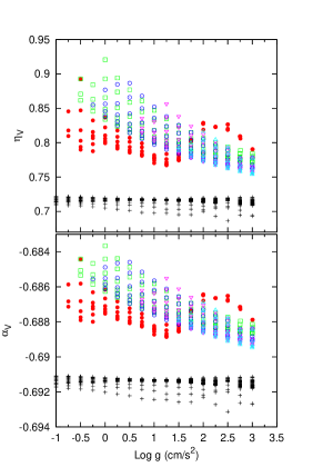
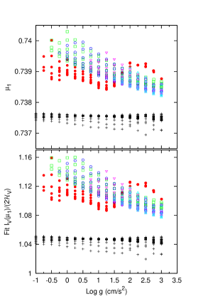
Figure 2: Surface gravity dependence of $\eta_{\lambda}$, $\alpha_{\lambda}$, fixed point $\mu_{1}$ and the normalized intensity at the fixed point, $I_{\lambda}(\mu_{1})/2\mathcal{H}_{\lambda}$, for the $V$ spectral band. Plane-parallel model atmospheres are denoted by black crosses, and spherical model atmospheres are represented by other symbols. Filled red circles are $T_{\mathrm{eff}}=3000$ K, open green squares 4000 K, open blue circles 5000 K, downward pointing magenta triangles 6000 K and upward pointing pale blue triangles are 7000 K.

Beginning with the plane-parallel models, the black crosses in the upper left plot of Fig. 2 shows that the $\eta$ parameter is nearly constant over a very wide range of surface gravity for the models being considered. As required by Eq. (6), the near constancy of $\eta$ causes the $\alpha$ coefficient also to be almost constant, as shown by the black crosses in lower left panel of Fig. 2. Next, as a result of Eq. (7), the fixed point, $\mu_{1}$, must be nearly constant, as shown by the black crosses in the upper right panel of Fig. 2. Finally, when the nearly constant $\mu_{1}$ is used in Eq. (2), the result is a nearly constant value of the normalized intensity at the fixed point. This conclusion is confirmed by the black crosses in the lower right plot of Fig. 2.

The spherically symmetric models are fundamentally different. The various colored symbols in the upper left plot in Fig. 2 confirms the result of Sect. 2.3 that the parameter $\eta$ does vary with surface gravity. It then follows from Eq. (6) that $\alpha$ must also vary, as shown by the colored symbols in the lower left plot. As before, Eq. (7) requires that the variation of $\alpha$ leads to the variation of $\mu_{1}$ shown by the colored symbols in the upper right plot of Fig. 2. Finally, this leads to the variation of the normalized intensity at the fixed point shown by the colored symbols in the lower right plot. For spherically symmetric models, the conclusion is that the location and intensity of the fixed point depend on the fundamental stellar parameters.

The beginning step of this logical chain, the dependence of $\eta$ on the atmospheric parameters, is physically reasonable. As shown in the upper left panel of Fig. 2, as $\log g$ decreases, $\eta$ increases towards unity, meaning that $\mathcal{P}\rightarrow J$. This is the result of the intensity profile becoming extremely centrally concentrated, or, equivalently, the atmospheric extension approaches the stellar radius. Because $\eta$ depends upon the extension of the atmosphere, so do $\alpha$, the fixed point $\mu_{1}$, and the intensity at the fixed point.

3 Parameterization of atmospheric extension

Figure 3: Extension parameter $R_{\star}/M_{\star}$ compared to the relative atmospheric extension, $\Delta R/R_{\star}$, derived for more than 3000 spherical models.

To explore further the results shown in Fig. 2, we replace $\log g$ by a more explicit representation of the extension of the stellar atmosphere, for which we adopt

$$\frac{\Delta R}{R_{\star}}\propto\frac{R_{\star}}{M_{\star}}.$$ (8)

This dependence is physically plausible because the extension is larger for stars of larger radius, but greater masses pull the atmospheres into a more compact configuration.

One way of deriving Eq. (8) begins with the definition of the pressure scale height,

$$H\equiv\frac{kT}{\mu m_{\mathrm{H}}g},$$ (9)

where $H$ is the distance over which the pressure changes by a factor of $e$, $k$ is the Boltzmann constant, $T$ is the gas temperature, $\mu$ is the mean molecular weight of the gas, $m_{\mathrm{H}}$ is the mass of the hydrogen atom, and the surface gravity $g=GM_{\star}/R^{2}_{\star}$. Using $H$ to represent the thickness of the atmosphere, the relative extension of the atmosphere is

$$\frac{\Delta R}{R_{\star}}=\frac{H}{R_{\star}},$$ (10)

both sides of which are dimensionless. Assuming that $T$ and $\mu$ are nearly constant over the distance $H$, the relative extension of the atmosphere becomes

$$\frac{\Delta R}{R_{\star}}\approx\frac{\rm{constant}}{R_{\star}M_{\star}/R^{2}_{\star}}\propto\frac{R_{\star}}{M_{\star}},$$ (11)

which is our expression.

To test the correlation of $R_{\star}/M_{\star}$ with the actual atmospheric extension, we use the Rosseland optical depth to determine for each of our several thousand spherical models the quantity $\Delta R/R_{\star}$, where $\Delta R$ is the physical distance from the location where $\tau_{\mathrm{Ross}}=1$ out to the location of where $\tau_{\mathrm{Ross}}=0.001$, which is slightly more than one pressure scale height, and $R_{\star}$ is the radius where $\tau_{\mathrm{Ross}}=2/3$. Figure 3 plots the extension parameter $R_{\star}/M_{\star}$ for each model versus that model’s $\Delta R/R_{\star}$. While there is a spread because $T$ and $\mu$ do vary over the distance $H$, it is obvious that $R_{\star}/M_{\star}$ tracks the actual extension of the models quite well.

Using $R_{\star}/M_{\star}$ to represent the atmospheric extension transforms Fig. 2 into Fig. 4, where the extension parameter for the plane-parallel models is determined by assuming a mass of $5\leavevmode\nobreak\ M_{\sun}$ and computing the radius for each model from its surface gravity. Figure 4 shows, as expected, that $\eta_{\lambda}$ is a tight function of $\log(R_{\star}/M_{\star})$, except for the models with $T_{\mathrm{eff}}=3000$ K. It follows, because of the connections established in Sec. 2, that all other quantities also depend on $R_{\star}/M_{\star}$. For plane-parallel atmospheres the quantities are nearly constant, as expected, and as they were found to be in Fig. 2. Therefore, the values of $\mu_{1}$ and $I_{\lambda}(\mu_{1})/2\mathcal{H}_{\lambda}$ depend on the fundamental stellar parameters $R_{\star}$ and $M_{\star}$. The deviation of the models with $T_{\mathrm{eff}}=3000$ K may be due to changes in the atmospheres at the lowest temperature.

Excluding the models with $T_{\mathrm{eff}}=3000\leavevmode\nobreak\ \mathrm{K}$, we fit for each waveband the dependence of $\mu_{1}$ and $I_{\lambda}(\mu_{1})/2\mathcal{H}_{\lambda}$ on $\log(R_{\star}/M_{\star})$ shown in Fig. 4 using the functional forms

$$\mu_{1}=C_{\mu}\left(\log\frac{R_{\star}}{M_{\star}}\right)^{2}+D_{\mu},$$ (12)

and

$$\frac{I_{\lambda}(\mu_{1})}{2\mathcal{H}_{\lambda}}=C_{\mathrm{I}}\left(\log\frac{R_{\star}}{M_{\star}}\right)^{2}+D_{\mathrm{I}}.$$ (13)

The values of $C_{\mu}$, $D_{\mu}$, $C_{\mathrm{I}}$, and $D_{\mathrm{I}}$ for these fits to the spherical models are given in Table 1 for the five wavebands $B,V,R,I$, and $H$. We include fits for models with effective temperatures $T_{\mathrm{eff}}=5000$ K and models within the effective temperature range of $4100-4300$ K ($T_{\mathrm{eff}}=4200\pm 100$ K). Equation (12) and Eq. (13) will be employed in later sections.

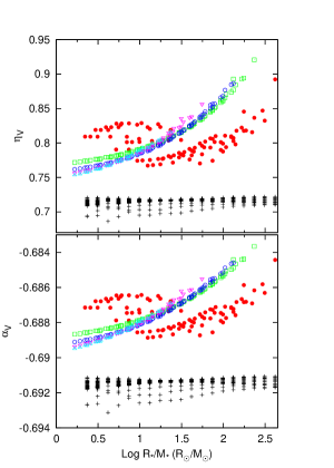
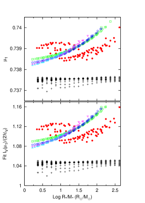
Figure 4: (Left) Values of the pseudo-moment $\eta_{\mathrm{V}}$ and variable $\alpha_{\mathrm{V}}$ as a function of atmospheric extension for spherical atmospheres, $R_{\star}/M_{\star}$ in solar units. (Right) The top panel shows the value of the primary fixed point, $\mu_{1}$, for the linear-plus-square-root parametrization, also plotted as a function of the extension of the spherical atmosphere. The bottom panel shows the dependence of the normalized $V$-band intensity of the fixed point on the atmospheric extension. The symbols have the same meaning as in Fig. 2. When comparing to Fig. 2, note that increasing extension corresponds to decreasing $\log g$.

Table 1: Best-fit coefficients for Eq. (12) and Eq. (13) as a function of $\log(R_{\star}/M_{\star})$ for various wavebands and effective temperatures.

$3000\leavevmode\nobreak\ \mathrm{K}<T_{\mathrm{eff}}\leq 8000\leavevmode\nobreak\ \mathrm{K}$
Band	$C_{\mu}$	$D_{\mu}$	$\sigma_{\mu}$
$B$	$2.5793\times 10^{-4}\pm 1.537\times 10^{-6}$	$0.738632\pm 3.163\times 10^{-6}$	$1.103\times 10^{-4}$
$V$	$2.9307\times 10^{-4}\pm 2.353\times 10^{-6}$	$0.738413\pm 4.841\times 10^{-6}$	$1.689\times 10^{-4}$
$R$	$3.1313\times 10^{-4}\pm 2.745\times 10^{-6}$	$0.738231\pm 5.648\times 10^{-6}$	$1.971\times 10^{-4}$
$I$	$3.4892\times 10^{-4}\pm 2.541\times 10^{-6}$	$0.738037\pm 5.229\times 10^{-6}$	$1.718\times 10^{-4}$
$H$	$4.4499\times 10^{-4}\pm 1.775\times 10^{-6}$	$0.737795\pm 3.652\times 10^{-6}$	$1.274\times 10^{-4}$
Band	$C_{\mathrm{I}}$	$D_{\mathrm{I}}$	$\sigma_{\mathrm{I}}$
$B$	$0.011800\pm 6.998\times 10^{-5}$	$1.09614\pm 1.440\times 10^{-4}$	$5.024\times 10^{-3}$
$V$	$0.013327\pm 1.070\times 10^{-4}$	$1.08622\pm 2.202\times 10^{-4}$	$7.683\times 10^{-3}$
$R$	$0.014227\pm 1.246\times 10^{-4}$	$1.07796\pm 2.563\times 10^{-4}$	$8.945\times 10^{-3}$
$I$	$0.015841\pm 1.151\times 10^{-4}$	$1.06914\pm 2.369\times 10^{-4}$	$8.268\times 10^{-3}$
$H$	$0.020205\pm 7.967\times 10^{-5}$	$1.05811\pm 1.639\times 10^{-4}$	$5.720\times 10^{-3}$
$T_{\mathrm{eff}}=4200\pm 100\leavevmode\nobreak\ \mathrm{K}$
Band	$C_{\mu}$	$D_{\mu}$	$\sigma_{\mu}$
$B$	$2.6004\times 10^{-4}\pm 1.800\times 10^{-6}$	$0.738675\pm 4.284\times 10^{-6}$	$3.907\times 10^{-5}$
$V$	$3.1320\times 10^{-4}\pm 1.325\times 10^{-6}$	$0.738436\pm 3.153\times 10^{-6}$	$2.876\times 10^{-5}$
$R$	$3.4835\times 10^{-4}\pm 1.332\times 10^{-6}$	$0.738240\pm 3.145\times 10^{-6}$	$2.868\times 10^{-5}$
$I$	$3.8848\times 10^{-4}\pm 1.255\times 10^{-6}$	$0.738009\pm 2.987\times 10^{-6}$	$2.724\times 10^{-5}$
$H$	$4.4270\times 10^{-4}\pm 1.088\times 10^{-6}$	$0.737803\pm 2.590\times 10^{-6}$	$2.362\times 10^{-5}$
Band	$C_{\mathrm{I}}$	$D_{\mathrm{I}}$	$\sigma_{\mathrm{I}}$
$B$	$0.011834\pm 8.423\times 10^{-5}$	$1.09813\pm 2.004\times 10^{-4}$	$1.828\times 10^{-3}$
$V$	$0.014247\pm 6.284\times 10^{-5}$	$1.08726\pm 1.495\times 10^{-4}$	$1.364\times 10^{-3}$
$R$	$0.015834\pm 6.260\times 10^{-5}$	$1.07837\pm 1.490\times 10^{-4}$	$1.358\times 10^{-3}$
$I$	$0.017644\pm 5.920\times 10^{-5}$	$1.06785\pm 1.409\times 10^{-4}$	$1.285\times 10^{-3}$
$H$	$0.020110\pm 4.964\times 10^{-5}$	$1.05847\pm 1.181\times 10^{-4}$	$1.077\times 10^{-3}$
$T_{\mathrm{eff}}=5000\leavevmode\nobreak\ \mathrm{K}$
Band	$C_{\mu}$	$D_{\mu}$	$\sigma_{\mu}$
$B$	$3.0649\times 10^{-4}\pm 1.646\times 10^{-6}$	$0.738567\pm 3.444\times 10^{-6}$	$1.717\times 10^{-5}$
$V$	$3.6147\times 10^{-4}\pm 1.400\times 10^{-6}$	$0.738322\pm 2.930\times 10^{-6}$	$1.461\times 10^{-5}$
$R$	$3.9658\times 10^{-4}\pm 1.665\times 10^{-6}$	$0.738146\pm 3.485\times 10^{-6}$	$1.737\times 10^{-5}$
$I$	$4.3136\times 10^{-4}\pm 2.098\times 10^{-6}$	$0.738956\pm 4.391\times 10^{-6}$	$2.188\times 10^{-5}$
$H$	$4.9064\times 10^{-4}\pm 2.630\times 10^{-6}$	$0.737752\pm 5.503\times 10^{-6}$	$2.743\times 10^{-5}$
Band	$C_{\mathrm{I}}$	$D_{\mathrm{I}}$	$\sigma_{\mathrm{I}}$
$B$	$0.013940\pm 7.913\times 10^{-5}$	$1.09320\pm 1.656\times 10^{-4}$	$8.254\times 10^{-4}$
$V$	$0.016429\pm 6.687\times 10^{-5}$	$1.08206\pm 1.399\times 10^{-4}$	$6.975\times 10^{-4}$
$R$	$0.018014\pm 7.665\times 10^{-5}$	$1.07407\pm 1.604\times 10^{-4}$	$7.995\times 10^{-4}$
$I$	$0.019579\pm 9.420\times 10^{-5}$	$1.06545\pm 1.971\times 10^{-4}$	$9.826\times 10^{-4}$
$H$	$0.022271\pm 1.138\times 10^{-4}$	$1.05616\pm 2.381\times 10^{-4}$	$1.186\times 10^{-3}$

4 Iterative method

The right panels of Fig. 4 show that $\mu_{1}$ and $I_{\lambda}(\mu_{1})/2\mathcal{H}_{\lambda}$ depend on $R_{\star}/M_{\star}$ for the spherical model atmospheres. It follows from the limb-darkening law, Eq. (2), that the coefficients $A_{\lambda}$ and $B_{\lambda}$ must also be functions of the atmospheric extension, which is confirmed in Fig. 5. Because the limb-darkening coefficients $A_{\lambda}$ and $B_{\lambda}$ in Eq. (2) can be derived from observations, this establishes an observational method for determining the atmosphere’s extension.

In Fig. 5 the open colored symbols show that the limb-darkening coefficients of stars with $T_{\mathrm{eff}}>3000$ K share a common dependence on the atmospheric extension for $\log(R_{\star}/M_{\star})\ga 1.5$ in solar units. This suggests it is possible to derive a unique value of $R_{\star}/M_{\star}$ for stars with atmospheric extensions $R_{\star}/M_{\star}\ga 30\ R_{\sun}/M_{\sun}$. Stars with $\log(R_{\star}/M_{\star})<1.5$ show a clear dependence on $T_{\mathrm{eff}}$.

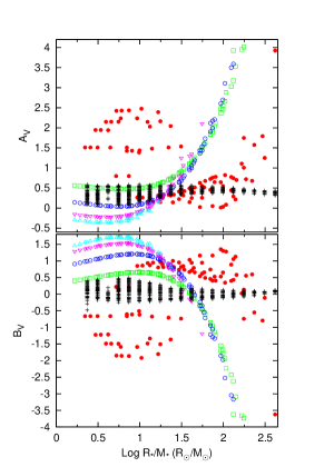
Figure 5: $V$-band values of the A limb-darkening coefficient (top panel) and the B limb-darkening coefficient (bottom panel) for the linear-plus-square-root parametrization given by Eq. (2), plotted as a function of the extension parameter, $R_{\star}/M_{\star}$ in solar units. The symbols have the same meaning as in Fig. 2.

The tight dependence of the $\mu_{1}$ and $I_{\lambda}(\mu_{1})/2\mathcal{H}_{\lambda}$ on $R_{\star}/M_{\star}$ displayed in Fig. 4 follows directly from Sect. 2.3, where we showed that $\mu_{1}$ is a function of $\alpha_{\lambda}$, which depends only on $\eta_{\lambda}\equiv\mathcal{P}_{\lambda}/J_{\lambda}$. The more scattered dependence of the coefficients $A_{\lambda}$ and $B_{\lambda}$ on the extension shown in Fig. 5 is due to these coefficients having a less direct functional dependence on the extension through the separate terms $J_{\lambda}/2\mathcal{H}_{\lambda}$ and $\mathcal{P}_{\lambda}/2\mathcal{H}_{\lambda}$, as we showed in Paper 1. Because of this, as we will show in the following sections, the values of $A_{\lambda}$ and $B_{\lambda}$ do not measure atmospheric extension as cleanly as using $\mu_{1}$ and $I_{\lambda}(\mu_{1})/2\mathcal{H}_{\lambda}$ as constraints.

Although $A_{\lambda}$ and $B_{\lambda}$ are less direct measures of the atmospheric extension, they are determined by the modeling of the lensing observations. Therefore, we propose an iterative method to use $A_{\lambda}$ and $B_{\lambda}$ to determine the atmospheric extension. The method begins by assuming an initial value for $\log(R_{\star}/M_{\star})$, which is used to compute $\mu_{1}$ with Eq. (12). This value of $\mu_{1}$ and the coefficients of the fit given in Table 1 enable us to compute the normalized intensity at the fixed point using Eq. (2). Finally, we compute a new value of $\log(R_{\star}/M_{\star})$ using Eq. (13). This new value of $\log(R_{\star}/M_{\star})$ replaces our initial assumption, starting a second iteration, which is continued until the value of $\log(R_{\star}/M_{\star})$ converges. If the stellar radius is determined by other methods, such as from interferometric observations and distance estimates, the converged value of $\log(R_{\star}/M_{\star})$ can be solved for the star’s mass.

5 Test using a model atmosphere

The previous section describes a potential method for determining the fundamental parameters of a star using stellar limb-darkening laws and the underlying physics behind these laws. To test this method, we arbitrarily selected a model with $T_{\mathrm{eff}}=5000$ K, $\log g=2$, $M_{\star}=5\leavevmode\nobreak\ M_{\sun}$, corresponding to $R_{\star}/M_{\star}=7.42\leavevmode\nobreak\ R_{\sun}/M_{\sun}$ or $\log(R_{\star}/M_{\star})=0.87$. Note that this value of the atmospheric extension falls in the region of Fig. 5 where the limb-darkening coefficients also depend on the $T_{\mathrm{eff}}$, whereas the fixed point and intensity in Fig. 4 are less dependent on the $T_{\mathrm{eff}}$. By selecting a trial model for which the $A_{\lambda}$- and $B_{\lambda}$-coefficients depend on $T_{\mathrm{eff}}$ as well as the atmospheric extension, we can determine how the iterative method is affected by this additional dependence. Table 2 lists the test model’s $A$ and $B$ limb-darkening coefficients for each of the five wavebands.

Table 2: Limb-darkening parameters and predicted $R_{\ast}/M_{\ast}$ for a model stellar atmosphere with $T_{\mathrm{eff}}=5000\leavevmode\nobreak\ \mathrm{K}$, $\log g=2$ and $M=5\leavevmode\nobreak\ M_{\sun}$.

Band	$A$	$B$	$R_{\star}/M_{\star}$	$\log g$
$B$	$0.613$	$0.507$	$6.65$	$2.09$
$V$	$0.048$	$1.206$	$6.46$	$2.12$
$R$	$-0.300$	$1.622$	$7.10$	$2.04$
$I$	$-0.642$	$2.051$	$7.28$	$2.02$
$H$	$-1.189$	$2.719$	$7.54$	$1.99$

Using the iterative method outlined in Sect. 4, we computed the $R_{\star}/M_{\star}$ for each waveband, with the results given in Table 2. By assuming a stellar radius of $R_{\star}=37.1\leavevmode\nobreak\ R_{\sun}$, we determined the surface gravity from $R_{\star}/M_{\star}$, which is also given in Table 2.

Even though the values of $A_{\lambda}$ and $B_{\lambda}$ for our test model have no observational uncertainty, the results in Table 2 differ slightly from the test model’s values. One reason for this difference is that the coefficients given in Table 1 have uncertainties because they are fits to a grid of thousands of models with the range of fundamental parameters given earlier; this leads to the spread of points shown in Fig. 4.

The variation with wavelength also contributes to the uncertainty. Averaging over all wavelengths, the mean difference of the predicted $R_{\star}/M_{\star}$ from the model’s value is only $5\%$, with the largest deviation being about 13% for the $V$-band. The wavelength variation of $R_{\star}/M_{\star}$ is related to the definition of the stellar radius, which we define as $R_{\star}=R(\tau_{\mathrm{Ross}}=2/3)$. However, in Table 2 the different wavelength bands produce values of $R_{\star}=R(\tau_{\mathrm{B,V,R,I,H}}=2/3)$, which will differ slightly from the radius where $\tau_{\mathrm{Ross}}=2/3$.

Using the five wavebands in Table 2, we find $(R_{\star}/M_{\star})_{\mathrm{avg}}=7.01\pm 0.45\leavevmode\nobreak\ R_{\sun}/M_{\sun}$, and $\log g_{\mathrm{avg}}=2.05\pm 0.05$, both of which are consistent with the actual values. Therefore, our proposed method for using limb-darkening coefficients recovers the actual stellar parameters for the theoretical test case with a statistical uncertainty of $\approx 8\%$ in $R_{\star}/M_{\star}$.

We improved the test by fitting simultaneously the limb-darkening coefficients for all the wavelength bands using the fix-point relations for all models with $T_{\mathrm{eff}}>3000$ K. This resulted in the best-fit values $R_{\star}/M_{\star}=6.83\pm 0.38\leavevmode\nobreak\ R_{\sun}/M_{\sun}$, and $\log g=2.04^{+0.02}_{-0.03}$, where the error bars come from the formal uncertainty of the fits to the coefficients in Table 1, which are used in Eq. (12) and Eq. (13). When the fit was repeated using only the relations for models with $T_{\mathrm{eff}}=5000$ K, the result was $R_{\star}/M_{\star}=7.61^{+0.22}_{-0.38}\leavevmode\nobreak\ R_{\sun}/M_{\sun}$ and $\log g=1.99^{+0.02}_{-0.01}$. We conclude from this test using a model stellar atmosphere that our proposed method for measuring stellar properties yields consistent results, although, as expected, the uncertainty of $R_{\star}/M_{\star}$ increases for stars with smaller atmospheric extension.

6 Conclusions

The purpose of this study has been to investigate how limb darkening probes fundamental stellar properties. The limb darkening was parameterized by a flux-conserving linear-plus-square-root law that has two free parameters that are functions of two angular moments of the intensity. The ratio of these two moments provides a measure of the amount of stellar atmospheric extension, represented by $R_{\star}/M_{\star}$. We tested our method for determining the extension from limb-darkening parameters using a spherically symmetric model atmosphere and found agreement of the mean value of the five spectral bands analyzed to within 8%.

We also find significant variation of $R_{\star}/M_{\star}$ due to the definition of the stellar radius. From the context of the model of the stellar atmosphere, we find it natural to define the stellar radius where $\tau_{\mathrm{Ross}}=2/3$, but other options are possible, such as $\tau_{\mathrm{Ross}}=1$ or using a specific wavelength, such as 500 nm, to define the radius where $\tau_{500}=1$. Observations, of course, are done in specific wavebands, such as $V$, and the stellar radius is assumed to refer to some particular optical depth, such as $\tau_{\mathrm{V}}=2/3$. Switching to another waveband will lead to another value of the radius. As an example, in the near-infrared the predicted radius is larger than at optical wavelengths. Therefore, the definition of the stellar radius is ambiguous in general for studies of angular diameters (e.g. Wittkowski et al., 2004, 2006b, 2006a), which makes the definition of the stellar radius challenging for stars with significant atmospheric extension. A recent example is Ohnaka et al. (2011), who measured the $K$-band angular diameter of Betelgeuse to be about 2 mas ($\approx$ 5%) smaller than measured by Haubois et al. (2009) in the $H$-band. However, simultaneously fitting $R_{\star}/M_{\star}$ to multiband limb-darkening observations provides a bolometric value for $R_{\star}/M_{\star}$ analogous to how spectrophotometry can be used to measure a star’s effective temperature.

The connection between atmospheric extension and stellar limb-darkening is a consequence of the assumption of spherical symmetry for the stellar atmospheres, not a unique feature of our SAtlas code. The results presented here should also be found using intensity profiles from spherically-symmetric Marcs models and the Phoenix model atmospheres used by Claret & Hauschildt (2003) and Fields et al. (2003). Unfortunately, in both of these works the authors truncated the intensity profiles to remove the low intensity limb and then redistributed the spacing of $\mu$-points. Truncating the intensity profile eliminates critical information about the limb darkening, and makes the star’s intensity distribution resemble a plane-parallel atmosphere, as we demonstrate in Fig. 6.

Figure 6: (a) Surface-brightness distribution as a function of fractional radius. The solid line is the full set of intensities from a spherical model atmosphere with $T_{\mathrm{eff}}=5000$ K, $\log g=2.0$ and $M_{\star}=5\leavevmode\nobreak\ M_{\sun}$. The dashed line has removed intensity values for $r/R_{\star}\geq 0.995$ and then renormalized the fractional radius to the interval $0-1$. The dotted line has removed intensity values for $r/R_{\star}\geq 0.98$ and then renormalized the fractional radius to the interval $0-1$. (b) Surface-brightness distributions from panel (a) plotted as a function of $\mu$, with the lines having the same meaning as in the (a) panel. (c) Fits to the surface-brightness distributions in panel (b) using Eq. (2). The lines have the same meaning as the other two panels.

Our method for determining fundamental stellar parameters is based on the general atmospheric properties of flux-conserving limb-darkening laws, not the particular law used here. For instance, Heyrovský (2003) and Zub et al. (2011) found a fixed point in flux-conserving linear limb-darkening laws, which indicates that the linear limb-darkening coefficient is a measure of the mean intensity and flux of the atmosphere. Another example is a quadratic limb-darkening law where the limb-darkening coefficients would provide a measure of the mean intensity and second moment of the intensity, $K$. Because these laws measure the correlation between various moments of the intensity in an atmosphere, they would also measure the atmospheric extension of that star.

We conclude that the method outlined in this work is a viable way to use a limb-darkening law, such as the linear-plus-square-root law employed here, to determine the fundamental physical parameters of stars. The method requires knowledge of one of the degenerate parameters effective temperature or luminosity. However, the method is able to constrain stellar parameters using limb-darkening observations even in the case when those limb-darkening observations from microlensing or eclipsing binaries cannot test the model stellar atmosphere directly. It seems as though we still have things to learn from fairly simple representations of limb darkening, and that, as observations continue to improve, this will become an even more powerful tool in the study of stellar astrophysics.