Improving multivariate Horner schemes with Monte Carlo tree search

Abstract

Optimizing the cost of evaluating a polynomial is a classic problem in computer science. For polynomials in one variable, Horner’s method provides a scheme for producing a computationally efficient form. For multivariate polynomials it is possible to generalize Horner’s method, but this leaves freedom in the order of the variables. Traditionally, greedy schemes like most-occurring variable first are used. This simple textbook algorithm has given remarkably efficient results. Finding better algorithms has proved difficult. In trying to improve upon the greedy scheme we have implemented Monte Carlo tree search, a recent search method from the field of artificial intelligence. This results in better Horner schemes and reduces the cost of evaluating polynomials, sometimes by factors up to two.

I Introduction

Polynomials are fundamental objects in mathematics and reducing the cost of evaluating polynomials is a classic problem in computer science. Applications abound, ranging from fast calculation on embedded devices and real-time calculations to high-energy physics (HEP), where one needs to perform Monte Carlo integrations of extremely large polynomials in many variables formcalc ; grace ; madgraph ; gosam . Numerous methods to optimize polynomial evaluation have been proposed, such as Horner’s method horner ; ceberio ; kojima , common subexpression elimination compilers , Breuer’s growth algorithm breuer ; hulzen and, recently, partial syntactic factorization leiserson .

For a polynomial in one variable, Horner’s method provides a computationally efficient form for evaluating it:

$$a(x)=\sum_{i=0}^{n}a_{i}x^{i}=a_{0}+x(a_{1}+x(a_{2}+x(\dots+x\cdot a_{n}))).$$ (1)

With this representation a dense polynomial of degree $n$ can be evaluated with $n$ multiplications and $n$ additions, giving an evaluation cost of $2n$. Here it is assumed that the cost of addition and multiplication are equal.

For multivariate polynomials Horner’s method can be generalized. To do so one chooses a variable and applies Eqn. (1), thereby treating the other variables as constants. Afterwards another variable is chosen and the same process is applied to the terms within the parentheses. This is repeated until all variables are processed. As an example, for the polynomial $a=y-3x+5xz+2x^{2}yz-3x^{2}y^{2}z+5x^{2}y^{2}z^{2}$ and the order $x<y<z$ this results in the following expression

$$a=y+x(-3+5z+x(y(2z+y(z(-3+5z))))).$$ (2)

Regarding the evaluation cost, the original expression uses 5 additions and 18 multiplications, while the Horner form uses 5 additions but only 8 multiplications. In general, applying a Horner scheme keeps the number of additions constant, but reduces the number of multiplications.

After transforming a polynomial with Horner’s method, the code can be further improved by performing a common subexpression elimination (CSE) compilers . In Eqn. (2), the subexpression $-3+5z$ appears twice. Eliminating the common subexpression results in the code

$$\begin{array}[]{l}T=-3+5z\\ a=y+x(T+x(y(2z+y(zT)))),\end{array}$$ (3)

which uses only 4 additions and 7 multiplications. The code optimization package Haggies reiter implements this method of Horner schemes followed by CSE.

Finding the optimal order of variables for the Horner scheme is still an open problem for all but the smallest polynomials, which are studied in Ref. kojima . Different orders may impact the cost of the resulting code, although no thorough study of this has been made to the authors’ knowledge. Simple algorithms have been proposed in the literature, such as most-occurring variable first, which results in the highest decrease of the cost at that particular step. This is also the order that is used in Haggies.

We studied the results of choosing different orders of variables for the Horner scheme and discovered that this order greatly affects the results, sometimes improving the cost by factors up to two. Unfortunately, most often it is impossible to perform an exhaustive search through all Horner schemes, since their number increases as the factorial of the number of variables. Therefore we have devised a method to find efficient orders by using Monte Carlo tree search (MCTS) chaslot ; browne , a recently proposed search method from the field of artificial intelligence.

II Monte Carlo tree search

MCTS is a best-first search method that uses random sampling to guide the traversal of the search tree. It has recently drawn much attention due to its application in the field of computer Go chaslot , a classic board game in which computers have traditionally played weakly. In the past decade the application of MCTS has improved the playing strength of computers from the level of advanced beginners to the level of strong amateur players. MCTS has also been applied successfully in numerous other games and optimization problems browne .

Figure 1: The asymmetric search through an MCTS search tree during the search for an efficient Horner scheme.

In MCTS the search tree is built in an incremental and asymmetric way, see Fig. 1. During the search the traversed part of the search tree is completely in memory. For each node MCTS keeps track of the number of times it has been visited and the estimated result of that node. At each step one node is added to the search tree according to a criterion that tells where most likely better results can be found. From that node an outcome is sampled and the results of the node and its parents are updated. This process is illustrated in Fig. 2. In more detail the four steps of the MCTS cycle are the following.

Selection During the selection step the node which most urgently needs expansion is selected. Several criteria are proposed, but the easiest and most-used is the UCT (upper confidence level for trees) criterion kocsis :

$$UCT_{i}=\left<x_{i}\right>+2C_{p}\sqrt{\frac{2\log{n}}{n_{i}}}.$$ (4)

Here $\left<x_{i}\right>$ is the average score of child $i$, $n_{i}$ is the number of times child $i$ has been visited and $n$ is the number of times the node itself has been visited. $C_{p}$ is a problem-dependent constant that should be determined empirically. Starting at the root of the search tree, the most-promising child according to this criterion is selected and this selection process is repeated recursively until a node is reached with unvisited children. The first term of Eqn. (4) biases in favor of nodes with previous high rewards (exploitation), while the second term selects nodes that have not been visited much (exploration). Balancing exploitation versus exploration is essential for the good performance of MCTS.

Expansion The selection step finishes with a node with unvisited children. In the expansion step one of these children is added to the tree.

Simulation In the simulation step a single possible outcome is simulated starting from the node that has just been added to the tree. This simulation can consist of generating a complete random outcome starting from this node or can be some known heuristic for the search problem. The latter typically works better if specific knowledge of the problem is available.

Backpropagation In the backpropagation step the results of the simulation are added to the tree, specifically to the path of nodes from the newly-added node to the root. Their average results and visit count are updated.

This MCTS cycle is repeated a fixed number of times or until the computational resources are exhausted. After that the best found result is returned.

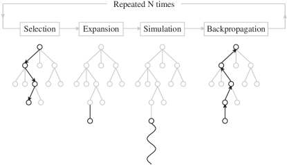
Figure 2: The Monte Carlo tree search cycle illustrated. (Figure from Ref. chaslot )

1:

2:function MCTSHorner

3:     r $\leftarrow$ new node with empty variable order

4:     for $i\leftarrow 1\dots$NumberOfTreeExpansions do

5:         $s\leftarrow$ select($r$)

6:         $s\leftarrow$ expand($s$)

7:         $x\leftarrow$ simulate($s$)

8:         backpropagate($s$,$x$)      

9:     return best optimized expression found

10:

11:function select($s$)

12:     while $s$ is fully expanded do

13:         $s\leftarrow\operatornamewithlimits{argmax}\limits_{\text{children }c\text{ of }s}\frac{x(c)}{n(c)}+2C_{p}\sqrt{\frac{2\log(n(s))}{n(c)}}$      

14:     return $s$

15:

16:function expand($s$)

17:     $o\leftarrow$ variable order of $s$

18:     $x\leftarrow$ random variable not in $o$

19:     $o\leftarrow$ append($o$,$x$)

20:     $c\leftarrow$ new node with variable order $o$

21:     add $c$ to children of $s$

22:     return c

23:

24:function simulate($s$)

25:     $o\leftarrow$ variable order of $s$

26:     while $o$ doesn’t contain all variables do

27:         $x\leftarrow$ random variable not in $o$

28:         $o\leftarrow$ append($o$,$x$)      

29:     $e\leftarrow$ HornerScheme(expression, $o$)

30:     $e\leftarrow$ CommonSubexpressionElimination($e$)

31:     return $\frac{\text{NumberOfOperations(expression)}}{\text{NumberOfOperations}(e)}$

32:

33:function backpropagate($s$,$\delta x$)

34:     while $s\neq$ null do

35:         $x(s)\leftarrow x(s)+\delta x$

36:         $n(s)\leftarrow n(s)+1$

37:         $s\leftarrow$ parent of $s$      

Algorithm 1 Pseudocode of MCTS Horner

III Efficient Horner schemes

In the existing code optimization packages that use Horner schemes combined with CSE, a simple algorithm for the order of the variables is chosen. Widely used is the occurrence order, where the variables are sorted with respect to the number of occurrences in the polynomial ceberio . The variable that has the largest number of occurrences comes first in the order and is the first one used in Horner’s method.

To test whether this algorithm gives efficient Horner schemes we took a large polynomial with 15 variables, a result from HEP calculations, and generated a million random orders which were used for Horner’s method followed by CSE. The occurrence order performed quite well, about a standard deviation above average, but far better orders were also found. An interesting feature of the orders that led to efficient schemes also showed up: these orders all shared the same variables in the trailing part of the order. These are the variables that eventually show up most often in the common subexpressions. These common subexpressions abound in the HEP polynomials due to much structure, such as combinations of coupling constants or dot products and masses.

Motivated by this observation we use MCTS to determine an order of the variables that gives efficient Horner schemes. The root of the search tree represents that no variables are chosen yet. This root node has $n$ children, with $n$ the number of variables. The other nodes represent choices for a number of variables in the trailing part of the order. This number equals the depth of the node in the search tree. A node at depth $d$ has $n-d$ children: the remaining unchosen variables.

In the simulation step the incomplete order is completed with the remaining variables added randomly. This complete order is then used for Horner’s method followed by CSE. The number of operations in this optimized expression is counted. The selection step uses the UCT criterion with as score the number of operations in the original expression divided by the number of operations in the optimized one. This number increases with better orders and is typically of ${\cal O}(1)$. The constant $C_{p}$ in Eqn. (4) must therefore be chosen of that size as well. Pseudocode of MCTS generated Horner schemes can be found in algorithm 1.

IV Results

To test the performance of this method an implementation is added to the computer algebra package Form form , which is widely used for HEP calculations. The results of this method are compared to a few existing algorithms. For comparison we added to Form optimization routines that use occurrence order Horner schemes followed by CSE. Furthermore, we compare to the open-source code optimization package Haggies reiter and the results from the paper on the hypergraph method based on partial syntactic factorization leiserson . We also tried the code optimization routines of Mathematica and Maple, but their results were not of particular interest. Finally, we present the results of the new code optimization routines of Form, which consist of MCTS generated Horner schemes followed by greedy optimizations. A detailed description of this algorithm will be presented in Ref. optimize . Since this algorithm is an extension of MCTS Horner with CSE, it should perform better.

	res(7,4)	res(7,5)	res(7,6)	HEP($\sigma$)	HEP($F_{13}$)	HEP($F_{24}$)
No optimizations	29 163	142 711	587 880	47 424	1 068 153	7 722 027
Occ. Horner + CSE	4 968	20 210	71 262	6 744	92 617	401 530
Haggies	7 540	29 125	101 821	13 214	238 093	crash
Hypergraph + CSE	4 905	19 148	65 770	—	—	—
MCTS + CSE	$(3.9\pm 0.1)\cdot 10^{3}$	$(1.5\pm 0.2)\cdot 10^{4}$	$(5.0\pm 0.6)\cdot 10^{4}$	$(4.3\pm 0.3)\cdot 10^{3}$	$(6.9\pm 0.4)\cdot 10^{4}$	$(4.4\pm 0.2)\cdot 10^{5}$
$[N=300]$	[$C_{p}=0.03$]	[$C_{p}=0.03$]	[$C_{p}=0.01$]	[$C_{p}=0.35$]	[$C_{p}=0.03$]	[$C_{p}=0.01$]
MCTS + CSE	$(3.86\pm 0.03)\cdot 10^{3}$	$(1.39\pm 0.01)\cdot 10^{4}$	$(4.58\pm 0.05)\cdot 10^{4}$	$4\,114\pm 14$	$(6.6\pm 0.2)\cdot 10^{4}$	$(3.80\pm 0.06)\cdot 10^{5}$
$[N=1\,000]$	[$C_{p}=0.1$]	[$C_{p}=0.07$]	[$C_{p}=0.05$]	[$C_{p}=0.75$]	[$C_{p}=0.2$]	[$C_{p}=0.015$]
MCTS + CSE	$(3.84\pm 0.01)\cdot 10^{3}$	$13\,786\pm 28$	$(4.54\pm 0.01)\cdot 10^{4}$	$4\,087\pm 5$	$(6.47\pm 0.08)\cdot 10^{4}$	$(3.19\pm 0.04)\cdot 10^{5}$
$[N=10\,000]$	[$C_{p}=0.2$]	[$C_{p}=0.2$]	[$C_{p}=0.15$]	[$C_{p}=1.5$]	[$C_{p}=0.3$]	[$C_{p}=0.03$]
MCTS + greedy	$(3.03\pm 0.03)\cdot 10^{3}$	$(1.09\pm 0.01)\cdot 10^{4}$	$(3.57\pm 0.01)\cdot 10^{4}$	$3\,401\pm 31$	$(4.63\pm 0.09)\cdot 10^{4}$	$(1.84\pm 0.04)\cdot 10^{5}$
$[N=10\,000]$	[$C_{p}=0.2$]	[$C_{p}=0.2$]	[$C_{p}=0.15$]	[$C_{p}=1.5$]	[$C_{p}=0.3$]	[$C_{p}=0.03$]

Table 1: The number of operations in the final expression after applying the optimization methods on the polynomials. The results for the hypergraph method are from Ref. leiserson ; we did not have the opportunity to test this method on the HEP polynomials. Different MCTS experiments are performed with different values for $C_{P}$, which are determined by trial and error. These are present in the table underneath their corresponding results. The MCTS results are statistical averages of different samples.

The polynomials to be optimized consist of two sets. The first set of polynomials (taken from Ref. leiserson ) are the resultants of two polynomials, $\text{res}_{x}(a(x),b(x))$, with $a(x)=\sum_{i=0}^{m}a_{i}x^{i}$ and $b(x)=\sum_{i=0}^{n}b_{i}x^{i}$, which is viewed as a polynomial in the $(m+n+2)$ variables $a_{i}$ and $b_{i}$. The second set consists of a number of large multivariate polynomials resulting from HEP calculations grace . For the set of resultants we observed that the variables that are factored out first in the Horner scheme are critical for the performance of MCTS Horner, as opposed to the last variables which are important for the HEP polynomials. This is probably due to many common subexpressions appearing in the HEP polynomials if the right variables are chosen last. The resultants don’t have that property and are probably more sensitive to a large decrease in the number of operations due to the Horner scheme itself. This conjecture must be investigated more rigorously. In the experiments for the resultants MCTS will search therefore for the best leading part of the variable order, while for the HEP polynomials it will search for the best trailing part.

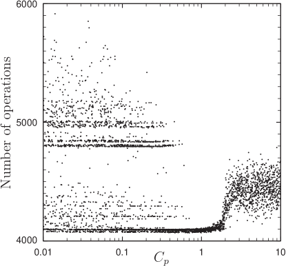
Figure 3: A scatter plot of the results of MCTS Horner with CSE with $3\,000$ tree expansions for the polynomial HEP($\sigma$) as a function of the constant $C_{P}$ that determines the balance between exploitation (small values) and exploration (large values). Shown are $4\,000$ randomly chosen values for $C_{p}$ with their corresponding results.

The results of the optimizations are expressed in the number of operations in the final expressions and are in Tab. 1. It is clear that MCTS Horner with CSE beats the existing algorithms, if the parameters (the exploitation/exploration constant $C_{p}$ from Eqn. (4) and the number of tree expansions $N$) are chosen properly.

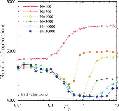
Figure 4: The results of MCTS Horner with CSE for the polynomial HEP($\sigma$) as function of the exploitation/exploration constant $C_{p}$ and the number of tree expansions $N$. All data points are statistical averages over at least 100 samples. The fourth line from above (green) consists of the average values per $C_{P}$ of the scatter plot of Fig. 3.

The effectiveness of MCTS depends heavily on the choice for these parameters. The results of MCTS with $3\,000$ tree expansions, followed by CSE, as a function of $C_{p}$ are in Fig. 3 for a large polynomial from HEP. For equal values of $C_{p}$ different results are produced because of different seeds of the random number generator. For small values of $C_{p}$, such that MCTS behaves exploitively, the method gets trapped in one of the local minima as can be seen from the different lines in the left-hand side of the figure. For large values of $C_{p}$, such that MCTS behaves exploratively, lots of options are considered and no real minimum is found as can be seen from the cloud of points on the right-hand side. For intermediate values of $C_{p}\approx 1$ MCTS balances well between exploitation and exploration and finds almost always a Horner scheme that is very close to the best one known to us.

The results of improving this polynomial for different numbers of tree expansions are shown in Fig. 4. For small numbers of tree expansions it turns out to be good to choose a low value for the constant $C_{p}$ (smaller than $0.5$). The search is then mainly driven by exploitation. MCTS quickly searches deep in the tree, most likely around a local minimum. This local minimum is explored quite well, but the global minimum is likely to be missed. With higher numbers of tree expansions a value for $C_{p}$ in the range $[0.5;2]$ seems suitable. This gives a good balance between exploring the whole search tree and exploiting the promising nodes. Really high values of $C_{p}$ seem a bad choice in general, since promising nodes are not exploited anymore. Note that these values hold for this particular polynomial, and that different polynomials give different optimal values for $C_{p}$ and $N$. The different values for $C_{p}$ in Tab. 1 are determined by trial and error and give decent results. With some more tuning even better results can probably be achieved. Automatic tuning of this parameter would be very convenient and is part of ongoing research.

Algorithm	Num. operations	Run time
No optimizations	142 711	—
Occurrence Horner + CSE	20 210	0.29 sec
Haggies	29 125	11.3 sec
Hypergraph + CSE	19 148	22.1 sec
MCTS+CSE $(N\!=\!300,C_{P}\!=\!0.03)$	$(1.5\pm 0.2)\cdot 10^{4}$	$47.4$ sec
MCTS+CSE $(N\!=\!10^{3},C_{P}\!=\!0.07)$	$(1.39\pm 0.01)\cdot 10^{4}$	$157$ sec
MCTS+CSE $(N\!=\!10^{4},C_{p}\!=\!0.2)$	$13\,786\pm 28$	$1.4\cdot 10^{3}$ sec
MCTS+greedy $(N\!=\!10^{4},C_{P}\!=\!0.2)$	$(1.09\pm 0.01)\cdot 10^{4}$	$1.4\cdot 10^{3}$ sec

Table 2: The run times of the various optimization algorithms on the polynomial $\text{res}(7,5)$. All tests are performed on 2.4GHz Pentium or Xeon CPUs.

The different algorithms vary a lot regarding the consumed computational resources, see Tab. 2. MCTS Horner with CSE needs considerably more run time than a greedy Horner scheme with CSE. This makes sense, because MCTS basically does such an operation per tree expansion. With only few computational resources available it is better to use a greedy Horner scheme than to use MCTS. If used it searches through the tree for good schemes for too short a time and does not find one, therefore resulting in a bad scheme. Compared to Haggies and the hypergraph method, MCTS with 300 expansions gives slightly longer run times for slightly better results. When the quality of the polynomial evaluation scheme is of great importance, it makes sense to spend more time to find a better evaluation scheme. With more time available, so that large parts of the search tree can be traversed, MCTS Horner with CSE or greedy optimizations outperforms all other methods considerably.

V Discussion

Polynomials are fundamental mathematical objects, naturally occurring at many places in mathematics and science. Efficient evaluation of polynomials is of great importance to many application areas. Horner’s method is a simple approach straight out of undergraduate algorithms textbooks. For something so basic, it is remarkable that over the years so little improvement has been made in finding more efficient evaluation schemes.

We improve on the traditional multivariate Horner schemes, where the variable order is fixed by a simple procedure, by employing MCTS. By statistically sampling the different variable orders it is designed to balance exploitation of known good schemes while not forgetting to explore unknown schemes as well.

The basic multivariate Horner schemes generated with most-occurring variables ordered first will quickly yield schemes that may be efficient enough for many applications. More demanding domains, where the expressions are large and/or evaluated many times, need better evaluation schemes. For these applications it pays to invest the time to generate them. MCTS is suitable for these types of applications. Evaluating large expressions for Feynman diagrams in HEP is one such domain, where large expressions have to be evaluated many times doing Monte Carlo integration formcalc ; grace ; madgraph ; gosam .

For all examined polynomials MCTS Horner, followed by CSE, generated evaluation schemes that were better than any other algorithm that we tried. A further analysis of the performance is ongoing research. This includes sensitivity analysis to different parameters (exploitation/exploration constant, number of tree expansions), dependence on the polynomial (size, number of variables, use of heading or trailing part of the variable order), automatic tuning of the parameters to the polynomial, better criteria for the selection step, possible heuristics for the simulation step (such as using the occurrence order instead of random completion), and the parallelization of the algorithm.

References

- (1) T. Hahn, M. Pérez-Victoria, Comput. Phys. Comm. 118 (1999) 153–165.
- (2) J. Fujimoto et al., Nucl. Phys. Proc. Suppl. 160 (2006) 150–154.
- (3) J. Alwall, JHEP 1106 (2011) 128.
- (4) G. Cullen et al., Eur. Phys. J. C72 (2012) 1889.
- (5) W.G. Horner, Phil. Trans. Soc. London (1819) 308–305. Reprinted in: D.E. Smith, A Source Book in Mathematics McGraw-Hill (1959)
- (6) M. Ceberio, V. Kreinovich, ACM SIGSAM Bull. 38 (2004) 8–15.
- (7) M. Kojima, J. Oper. Res. Soc. Japan 51 (2008) 29-–54.
- (8) Aho, Sethi, Ullman, Compilers: Principles, Techniques and Tools, Addison Wesley (1986).
- (9) M.A. Breuer, ACM Commun. 12 (1969) 333–340.
- (10) J.A. van Hulzen, LNCS 162 (1983) 286–300.
- (11) C.E. Leiserson, L. Li, M.M. Maza, Y. Xie, LNCS 6327 (2010) 342–353.
- (12) T. Reiter, Comput. Phys. Commun. 181 (2010) 1301-1331.
- (13) G.M.J.B. Chaslot, Monte-Carlo Tree Search, PhD thesis (2010).
- (14) C.B. Browne et al, IEEE Trans. Comput. Intell. AI Games 4 (2012) 1–43.
- (15) L. Kocsis, C. Szepesvári, LNCS 4212 (2006) 286–293.
- (16) J. Kuipers, T. Ueda, J.A.M. Vermaseren, J. Vollinga, FORM version 4.0, preprint: arXiv:1203.6543 (2012).
- (17) J. Kuipers, J.A.M. Vermaseren, Code Optimization in FORM, in preparation.