Charge-Density Wave and One-dimensional Electronic Spectra in Blue Bronze: Incoherent Solitons and Spin-Charge Separation

Abstract

We present new high resolution angle resolved photoemission (ARPES) data for K_0.3MoO₃ (blue bronze) and propose a novel theoretical description of these results. The observed Fermi surface, with two quasi-one-dimensional sheets, is consistent with a ladder material with a weak inter-ladder coupling. Hence, we base our description on spectral properties of one-dimensional ladders. The marked broadening of the ARPES lineshape, a significant fraction of an eV, is interpreted in terms of spin-charge separation. A high energy feature, which is revealed for the first time in the spectra near the Fermi momentum thanks to improved energy resolution, is seen as a signature of a higher energy bound state of soliton excitations on a ladder.

Systems of two coupled chains (called ladders) can be viewed as a first step in crossing over from one dimension (1D), with its exotic physics of Luttinger liquid and spin-charge separation, to higher dimensions. In spite of being unusual and seemingly enigmatic, this 1D physics is now well understood, thanks to remarkable progress in applying field theoretic methods in condensed matter tsvelik_book . How this physics transforms in the course of crossover to higher dimension is why ladders have been intensely studied. While theoretical progress on this problem has been considerable, with work in predicting rich excitation spectra, dynamical generation of spectral gaps, existence of preformed pairs fabrizio ; fisher ; schulz ; Khev ; konik2 ; varma ; controzzi ; lee ; furusaki ; wu ; noack ; jeckelmann ; weihong ; poilblanc ; 2leg , the progress on the experimental side has been slower both due to limited numbers of materials with a suitable structure and limited experimental accuracy.

The molybdenum blue bronzes, A_0.3MoO₃ are among the most interesting and intensely studied examples of quasi-1D conductors Greenblatt ; Monceau2012 . They feature MoO₆ octahedra forming an array of weakly coupled pairs of conducting ladders Graham . According to band structure calculations the chemical potential is crossed by two slightly warped bands with 3/4-filling Canadell ; Mozos . These are bonding (B) and anti-bonding (AB) bands arising from the electron hopping between the two legs of a given ladder, with Fermi wave vectors $K_{FB}$ and $K_{FAB}$, respectively. The resulting Fermi surface nesting suggests a charge density wave (CDW) formation with a wave vector $K_{FB}+K_{FAB}$ along the chains.

In K_0.3MoO₃ a 3D phase transition into a charge-ordered insulating phase takes place at a temperature T${}_{CDW}\approx 180$K Johnston ; Kwok even though the magnetic susceptibility starts to decrease well above the transition, experiencing a one-third drop in the interval between 700K and 180K Johnston . The low-energy lattice responses measured in neutron and X-ray experiments also show precursor effects up to at least $\sim 2$T_CDW Monceau2012 ; Pouget ; Fleming1985 ; Sato . Previous angle-resolved photoemission (ARPES) measurements, while confirming the band structure predictions, also found significant breadth of the electronic spectra, extending to photoelectron energies $\sim$ eV Fedorov ; Perfetti ; Ando . By virtue of the lattice involvement in the CDW formation, this surprising incoherence was assigned to electron-phonon interactions and small polarons, in spite of the marked mismatch in the energy scales.

Here we report the results of new high resolution ARPES measurements of K_0.3MoO₃, which we analyze based on the electronic spectral properties of ladders. With much improved instrumental resolution, we focus upon examining the fine structure of the measured photoemission spectra. We resolve for the first time two broad peaks in regions of the Brillouin zone near the Fermi vector, dispersing through energies a significant fraction of an eV. We interpret these features as ladder excitations originating from the same interaction that underpins the 3D charge order existing in this material at low temperatures. The breadth of these peaks arises from the presence of gapless charge excitations (holons) and gapful spin solitons (spinons) with markedly different velocities. We obtain a good description of the measured spectra with two SU(2) Thirring models describing the spectral properties of a ladder, thus assuming that the physics is electron-driven and the electron-lattice interaction plays only a secondary role.

The K_0.3MoO₃ single crystals were grown by an electrolytic reduction method Li . High resolution angle-resolved photoemission measurements were carried out with a Scienta R4000 electron energy analyzer Liu . For the band structure measurements and Fermi surface mapping (Fig. 1), we used a helium discharge lamp as the light source with a photon energy of $h\nu$ =21.218 eV. The overall energy resolution was set at 10 meV and the angular resolution was 0.3^∘, corresponding to a momentum resolution of 0.0091 Å^-1 at the photon energy of 21.218 eV. For the high-precision ARPES measurements (Fig. 2 and Fig. 3), a vacuum ultra-violet (VUV) laser with a photon energy $h\nu$=6.994 eV was used as a light source. The energy resolution in this case was 1 meV. The angular resolution is 0.3^∘, corresponding to a momentum resolution of 0.004 A^-1 at the photon energy of 6.994 eV. The Fermi level is referenced from measuring a clean polycrystalline gold that is electrically connected to the sample. The crystal was cleaved in situ and measured in vacuum with a base pressure $\lesssim 5\times$10^-11 Torr.

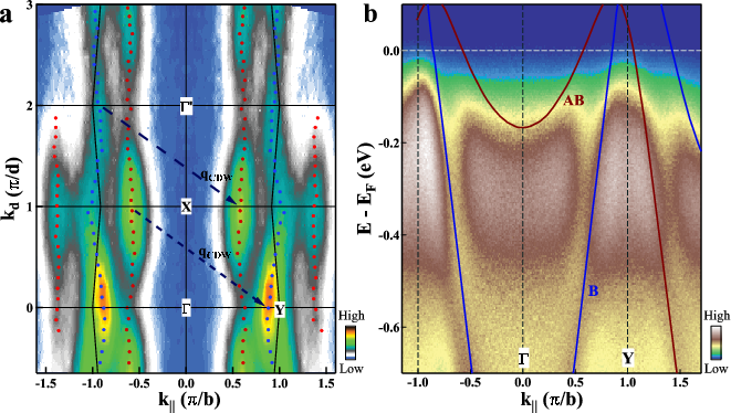
Figure 1: a) The measured Fermi surface of K_0.3MoO₃. Data are symmetrized with respect to the k_||=0 line. Blue and red dots show the extracted Fermi momentum along the Fermi surface sheets. The CDW vectors are marked by the dashed arrows. b) The measured band structure along $\Gamma$-Y (k_d = 0) showing two bands, the bonding (B) and the anti-bonding (AB) ones, crossing the Fermi level. The solid lines mark bands predicted from band structure calculations Mozos .

Fig. 1a shows the bare Fermi surface (FS) map measured at 80 K. The FS is open and consists of weakly warped sheets (blue and red dots in Fig. 1a). This warping arises from a weak interladder hopping, $t_{\perp}\approx 100$ meV (to be compared with the hopping between the legs of a given ladder, $t_{\rm rung}\approx 500$ meV). Fig 1b shows the band structure measured along the $\Gamma$-Y cut at 80 K. At energies less than 1eV we clearly distinguish two bands (B and AB). The non-interacting bands cross the chemical potential at 0.97 $\pi$/b, 0.6 $\pi$/b, -0.55 $\pi$/b and -0.96 $\pi$/b, consistent with the band structure calculations in Ref. Mozos, and previous ARPES measurements Fedorov ; Perfetti ; Ando . The Fermi surface nesting vector is thus estimated to be $\approx$ 1.52 $\pi$/b, also in good agreement with the measured CDW vector Pouget ; Fleming1985 ; Sato .

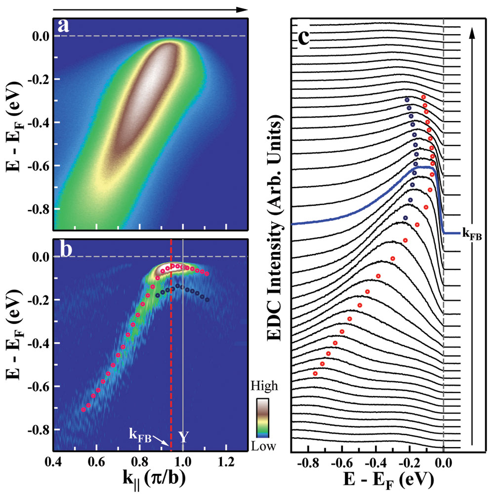
Figure 2: a) The band structure along $\Gamma$-Y momentum cut measured with 1 meV energy resolution. Due to ARPES matrix element effects, the AB band intensity is suppressed. b) Second derivative with respect to energy of the data in (a). Two structures around k_FB, corresponding to incoherent soliton and bound state (see text), are clearly seen. c) The corresponding photoemission spectra (EDCs). Red (blue) circles mark in b) and c) the dispersion of the soliton and the bound state, respectively, both for the B and the weak AB band.

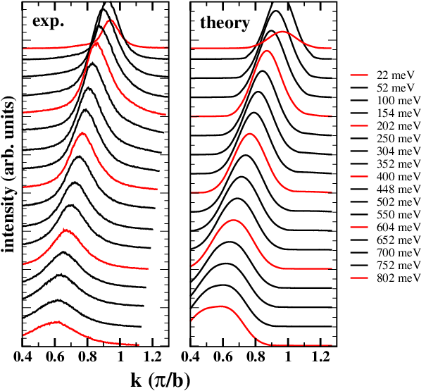
Figure 3: The MDCs for different binding energies obtained from the data in Fig. 2 (left) and the theoretical prediction for these MDCs (see the text) and accounting for the surface inhomogeneity of the Fermi wave vector.

In Fig. 2 we present high resolution laser ARPES data for the band structure along the ladder. Due to the effects of matrix elements, the B band is more clearly visible than the AB band (Fig. 2a). Its electronic structure exhibits two features, seen as excitation branches near $K_{FB}$, clearly distinguished in the second derivative image (Fig. 2b). The lower binding-energy branch was observed in earlier measurements Fedorov ; Perfetti ; Ando , while the higher energy branch has not hitherto been resolved. The lower branch, starting at $\approx 60$ meV below $E_{F}$, reaches binding energy $\approx 0.8$ eV as $k_{||}$ varies from $\pi/b$ to 0.4 $\pi/b$ (red circles in Fig. 2b). The second branch with a lower spectral weight starts at $E-E_{F}\approx-150$ meV, remains distinct until roughly $\approx-200$ meV, and then merges with the first branch (blue circles in Fig. 2b). The two branches gradually become indistinguishable when the temperature increases so that at 240 K only one broad hump is observed (see supplementary material supp ). We argue that the lower branch is due to the smeared contribution of the holon and spinon to the ARPES signal while the upper branch is due to a spinon plus a coherent excitation formed as a bound state of two spinons.

A further feature not previously seen is the left-right asymmetry of the low energy branch: the slope of the band on the right side of the Fermi momentum ($k_{||}>K_{FB}$) $v_{R}\approx$ 1.15 eV$\AA$ is smaller than that on the left side ($k_{||}<K_{FB}$): $v_{L}\approx$ 5.33 eV$\AA$. These roughly correspond to the expected velocities of the B and AB bands Mozos . We argue that both the presence of two excitation branches and the asymmetry of their dispersion can be explained in terms of 1D intra-ladder interactions.

The previous attempts to explain the broad ARPES spectrum have been based on small polaron theory Perfetti ; Roscha . However, the shear size of the gaps and the energy dependence of the incoherence peaks’ widths, running to a significant fraction of an eV, suggests that these features have an electronic origin. Here we present non-perturbative calculations for the ARPES response. Before presenting theoretical details, we present in Fig. 3 the momentum distribution curves (MDCs) obtained by cutting the measured ARPES spectra at a number of different binding energies and our theoretical predictions for these MDCs. We see an impressive fit between the two.

We adopt an approach where we consider an interacting ladder as the basis for calculations, treating it using powerful 1D non-perturbative techniques, and then considering interladder interactions as a perturbation Essler2002 ; Essler2005 ; Konik . In order to account for the experimental observations, we devise a low energy theory that (i) maximizes the fluctuations leading to the observed incoherency of the ARPES lineshapes and (ii) gives rise to a zero temperature CDW instability at $k_{FB}+k_{FAB}$ which, in the presence of 3D coupling, is shifted to finite temperatures. Since the CDW instability occurs at the wave vector $k_{FB}+k_{FAB}$, both bands are involved in its creation. However, as is clearly seen on Fig. 1b, these bands have very different Fermi velocities $v_{FB}$ and $v_{FAB}$ - a feature that is not present in standard theories of ladders. This velocity difference precludes the emergence of an SO(6) symmetry, which is one of the most interesting predictions of the low energy theory of ladders fisher ; schulz . Nevertheless, we will argue that a remnant of this symmetry remains in the form of an electron-hole bound state.

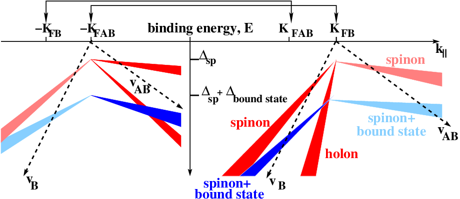
Figure 4: Schematics of interaction between pairs of Fermi points, ($K_{FB},-K_{FAB}$) and ($K_{FAB},-K_{FB}$). For the first pair we show the asymmetry in the dispersion on either side of these two Fermi points. The color bars locate the contributions in $(k,E)$ of the various excitations (holon (red), spinon (red), spinon + bound state (blue)) to the ARPES signal, with the intensity of the color corresponding to the intensity of the ARPES signal.

Since the spectral gaps are much smaller than the bandwidth, it is reasonable to linearize the dispersion close to the Fermi points by introducing slowly varying right- and left-moving components of the fermionic fields

$$\psi_{j\sigma}=\mbox{e}^{-ik_{Fj}x}\psi_{Rj\sigma}+\mbox{e}^{ik_{Fj}x}\psi_{Lj\sigma},~{}~{}j=B,AB.$$ (1)

Because of the different Fermi velocities in the bonding and anti-bonding bands, we expect the theory will not have a symmetry higher than U(1)$\times$SU(2). Moreover, we expect the strongest interaction to occur between the bonding and anti-bonding bands, foreshadowing the rise of the observed 3D CDW order. To this end we consider a model where the fermions at $K_{FB}$ interact with the fermions at $-K_{FAB}$ and similarly those at $-K_{FB}$ interact with fermions at $K_{FAB}$. This leads us to describe the system as two decoupled 1D theories, $H=H_{1}+H_{2}$:

$$H_{1}\! = \!\!-i\int\!\!dx\big{(}v_{FB}\psi^{\dagger}_{Rp\sigma}\partial_{x}\psi_{Rp\sigma}\!-\!v_{FAB}\psi^{\dagger}_{LAB\sigma}\partial_{x}\psi_{LAB\sigma}\big{)}$$ (2)

$$+ \sum_{l,l^{\prime}=R,L}g_{ll^{\prime}0}\rho_{lB}\rho_{l^{\prime}AB}+g_{ll^{\prime}}J^{a}_{lB}J^{a}_{l^{\prime}AB};$$ (3)

$$\rho_{lp} = \psi^{\dagger}_{lp\sigma}\psi_{lp\sigma},~{}~{}J^{a}_{lp}=\psi^{\dagger}_{lp\sigma}\tau^{a}_{\sigma\sigma^{\prime}}\psi_{lp\sigma^{\prime}};$$ (4)

with $H_{2}=H_{1}(AB\leftrightarrow B)$ and where $\tau^{a}$ are Pauli matrices. The coupling constants $g_{ll}$ and $g_{0ll}$ renormalize the spin and charge velocities (see Ref. supp ). On the other hand the couplings $g_{LR},g_{0LR}$ determine the presence of spin and charge gaps. $g_{LR}$ is equal to the $K_{FB}+K_{FAB}$ Fourier component of the renormalized Coulomb interaction. We take it to be positive, corresponding to an attractive interaction that is necessary for CDW formation. It leads to a spinon mode with gap $\Delta\sim 0.1\Delta_{1/2}$ esskon where $\Delta_{1/2}\sim W(g_{LR}/v_{Av})^{1/2}\exp(-\pi v_{Av}/g_{LR})$ review (with $v_{Av}=(v_{FB}+v_{FAB})/2$) is the putative gap at 1/2 filling. We assume $g_{0LR}$ is negative, consistent with gapless holons. The magnitudes of these various couplings mark blue bronze as moderately interacting supp .

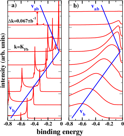
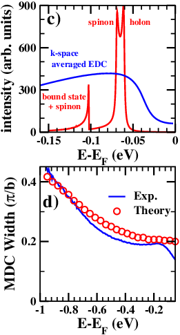
Figure 5: a) and b): EDCs for the B band for k-vectors ranging from $k=0.64\pi b^{-1}$ to $k=1.17\pi b^{-1}$: a) before averaging for differential surface doping; b) after averaging with a Gaussian of width $0.07\pi b^{-1}$. c) Different contributions to EDC at $k=0.94\pi b^{-1}$: holon, spinon, and spinon and bound state. d) Comparison of MDC width between theory and experiment.

The spectral function corresponding to this theory can be obtained from the one for the case of equal Fermi velocities Essler2002 by a Galilean transformation: $t^{\prime}=t,~{}~{}x^{\prime}=t\Delta v+x,~{}~{}\Delta v=(v_{FB}-v_{FAB})$. The corresponding retarded Green function is

$$G_{RB}(\omega,k)\!\! = \!\!\langle\psi_{Rb\sigma}\psi^{\dagger}_{Rb\sigma}\rangle(\omega,k)\!=\!\frac{2Z}{1+\alpha}F(\omega-k\Delta v/2,k);$$ (5)

$$F(\omega,k)\! = \!\frac{\tilde{\omega}+v_{c}k}{\Delta^{2}+v^{2}_{c}k^{2}-\tilde{\omega}^{2}}\Big{[}\big{(}\Delta+\sqrt{\Delta^{2}+v_{c}^{2}k^{2}-\tilde{\omega}^{2}})^{2}$$ (7)

$$\hskip 36.135pt-\frac{1-\alpha}{1+\alpha}(\tilde{\omega}+v_{c}k)^{2}\Big{]}^{-1/2},$$

where $Z\sim 1$, $v_{c,s,\pm}=v_{c,s}\pm\Delta v/2$, $\alpha=v_{s}/v_{c}$, and $\tilde{\omega}=\omega+i\delta$. We can use the measured $v_{L}$ and $v_{R}$, the velocities to the left and right of $k=K_{FB}$, to infer $v_{s}$ and $v_{c}$ (see supp ).

The most notable prediction is that the spectral features on different sides of any Fermi point disperse with different velocities. This is illustrated schematically in Fig. 4 for the pair of Fermi points $K_{FB}$ and $-K_{FAB}$. We also see the observed asymmetry on the spectrum in Fig. 5 where we plot the expected line shapes for a set of EDCs for different k’s in the vicinity of $K_{FB}$: for $k<K_{FB}$ the spectral weight disperses with velocity $v_{FB}$ while for $k>K_{FB}$ the spectral weight, while much reduced, disperses with velocity $v_{FAB}$.

We have so far ignored interactions between fermions living at $K_{FB},-K_{FAB}$ and $-K_{FB},K_{FAB}$. However, such interactions are present even though they are weaker than those responsible for the 3D CDW order. In a ladder system with equal velocities in the bonding and anti-bonding bands, the theory governing the low energy response has a dynamically generated SO(6) symmetry, and so predicts that there will be a bound state of the spin degrees of freedom of the electrons schulz ; esskon . This bound state leads to a feature at an energy $\omega=(1+\sqrt{2})\Delta$ for $k=K_{FB},K_{FAB}$, above the single particle gap, $\Delta$, in the spectral function. While in a theory with broken SO(6) symmetry (i.e., $v_{B}\neq v_{AB}$) we cannot predict where exactly this threshold will occur, we expect that this bound state will survive symmetry breaking, as a consequence of the bound state having significant binding energy. We believe that the contribution to the spectral function coming from this bound state is responsible for the band of intensity at higher binding energy in Fig. 2b (the blue dots). In Fig. 4 we schematically illustrate all of the contributions, holon, spinon, and spinon plus bound state, to the spectral function.

In Fig. 5a and 5c, we see how spin-charge separation leads to broadened features in the ARPES lineshape giving rise to two singularities in the spectral weight at an upper and a lower energy that disperse with different velocities (the spin and charge velocities) as $k$ moves away from the Fermi point. We also see how the bound state plus spinon makes a distinct contribution to the spectral function. (Our estimate of the contribution here made by the bound state is based on the symmetric SO(6) theory - see supp ). At $k$ near $K_{FB}$ this contribution appears at energies higher than the spinon and holon edges (Fig. 5c). But as $k$ moves away from $K_{FB}$ this second contribution merges into the initially lower holon edge (Fig. 5a). This is precisely the behavior we observe in Fig. 2a.

However, different spin and charge velocities alone cannot explain the broad linewidths observed. Fig. 5d shows that the experimental widths of the momentum distribution curve (MDCs) saturate to a value of about $0.18\pi b^{-1}$ at low binding energies. We believe that additional broadening of ARPES spectra arises from charge inhomogeneities present on the surface of K_0.3MoO₃, which is a poor conductor. They generate a nearly rigid shift of the surface bands Monceau2012 and will lead to ladders in different regions on the surface of the sample to be at different dopings, in turn leading to a spatial dependence of $K_{FB}$ and $K_{FAB}$. Such inhomogeneities were observed in a scanning tunneling microscopy study of a sister blue bronze Rb_0.3MoO₃ Brun ; Monceau2012 , where $K_{F}$ was found to vary across the surface from about $0.65b^{*}$ to about $0.80b^{*}$ ($b^{*}=2\pi/b$). The ARPES measurements on the 1D Mott-Hubbard insulator, SrCuO₂, considered the best evidence for spin-charge separation, also yield broad peaks much broader than the corresponding theoretical prediction (see Fig. 3 in Kim ). Hence, we believe that such broadening is an inherent feature of ARPES measurements on poorly conducting systems.

To account for these additional broadening effects, we convolve the lineshapes with a Gaussian of width $=.07\pi b^{-1}$ (Fig. 3, Fig. 5b and 5c). A considerable increase in broadening accounts very well for the experimental lineshapes, leading to a flat but finite MDC width at low energies while at higher energies the MDC widths grows as would be expected in a system with differing spin and charge velocities, Fig. 5d. Our theory thus accounts for the experimental MDC width at both low and high energies.

In conclusion, we have presented high resolution ARPES data for the CDW material K_0.3MoO₃. Using non-perturbative field theoretic techniques, we have argued that the features in the ARPES lineshapes can be understood primarily as arising from electronic correlations. Narrowily drawn, this treatment has implications for the theory of cuprate ladders. In particular, our prediction of a bound state signature will apply to the ARPES response, already measured yoshida , of such ladders. More broadly drawn, this finding suggests that electronic interactions may play a similarly important role in other materials exhibiting CDW-like order, from the chalcogenides to the maganites to stripe ordered cuprates.

I Supplementary material: Incoherent Soliton Excitations and Spin-Charge Separation in Blue Bronze

I.1 Determination of Spin and Charge Velocities

To determine the spin and charge velocities we begin with the experimental determination of the velocities for $k_{||}>K_{FB}$, $v_{R}=0.47$eV$b\pi^{-1}$ and $k_{||}<K_{FB}$, $v_{L}=2.16$eV$b\pi^{-1}$. (Here b is the lattice spacing.) For $k_{||}<K_{FB}$ we assume that the spectral response sees roughly equal contributions from the the spinon and the holon (consistent with our theoretical analysis), and so the measured velocity is a arithmetic mean of the spinon and holon velocities:

$$v_{L}=\frac{v_{sL}+v_{cL}}{2}.$$ (8)

By how the MDC width grows with increasing binding energy (see Fig. 5d), we can estimate the difference of $v_{cL}$ and $v_{sL}$ :

$$v_{sL}-v_{cL}=1.49{\rm eV}b\pi^{-1}$$ (9)

This gives the spin and charge velocities for $k_{||}<K_{FB}$ as

$$v_{sL}=2.91{\rm eV}b\pi^{-1};~{}~{}~{}v_{cL}=1.42{\rm eV}b\pi^{-1}.$$ (10)

For $k_{||}>K_{FB}$, we assume the spectral response is dominated by the branch with the lesser velocity, again consistent with our theoretical analysis, in this case the holon. Thus it is this velocity that is directly measured:

$$v_{cR}=v_{R}=0.47eVb\pi^{-1}.$$ (11)

To determine the charge velocity $v_{cR}$ for $k_{||}>K_{FB}$ we resort to a theoretical analysis. This gives the spin and charge velocities in terms of the (bare) velocities of the bonding ($v_{B}$) and anti-bonding ($v_{AB}$) bands and the effective zero frequency component of the Coulombic interaction, $V(0)$, as tsvelik_book

$$v_{cL} = v_{Av}(1+\frac{V(0)b}{2\pi v_{Av}})+\frac{\Delta v}{2};$$ (12)

$$v_{sL} = v_{Av}(1-\frac{V(0)b}{2\pi v_{Av}})+\frac{\Delta v}{2};$$ (14)

$$v_{cR} = v_{Av}(1+\frac{V(0)b}{2\pi v_{Av}})-\frac{\Delta v}{2};$$ (16)

$$v_{sR} = v_{Av}(1-\frac{V(0)b}{2\pi v_{Av}})-\frac{\Delta v}{2}.$$ (18)

where

$$v_{Av} = \frac{v_{B}+v_{AB}}{2};$$ (19)

$$\Delta v = v_{B}-v_{AB}.$$ (21)

Using these relations we can then determine the remaining unknown velocities as well as $V(0)$:

$$v_{sR}=1.96{\rm eV}b\pi^{-1};~{}~{}v_{B}=2.16{\rm eV}b\pi^{-1};~{}~{}v_{AB}=1.21{\rm eV}b\pi^{-1};~{}~{}V(0)=-1.49eV.$$ (22)

We see that our analysis gives a value of $V(0)$ consistent with blue bronze being only moderately interacting. It’s negative value is consistent with (and necessary for) their being a gap in the spin sector tsvelik_book .

We can also show that the energy scale set by $V(0)$ governs the size of the gap of the spinons. The spinon gap is given by $\Delta\sim 0.1\Delta_{1/2}$ esskon where $\Delta_{1/2}\sim W(g_{LR}/v_{Av})^{1/2}\exp(-\pi v_{Av}/g_{LR})$ review is the gap at half filling. The prefactor $0.1$ relating the gap at 3/4-filling to the gap at 1/2-filling is a rough estimate based on an $SO(6)$ symmetric theory. Nonetheless we feel it is accurate to within a factor of 2. While $g_{LR}\sim bV(K_{FAB}+K_{FB})$ involves the $K_{FAB}+K_{FB}$ Fourier component of the Coulomb interaction, it is reasonable to suppose this component is of the same magnitude of $V(0)$. This then gives $\Delta_{1/2}\sim W/2$ and so in turn $\Delta\sim W/20$. Taking the bandwidth $W$ as $~{}1eV$, we see that it makes a reasonable prediction for the magnitude of the observed spinon gap of $\sim 60meV$.

I.2 Description of the Contribution of the Spectral Response from the Bound State

To describe the contribution of the spectral response coming from the bound state we employ a description of the ladders appropriate where the Fermi velocities, $v_{AB}$ and $v_{B}$, of the ladders’ two bands are equal. We do so because then at low energies the low energy description of the doped ladders schulz ; esskon admits a field theoretic reduction governed by an SO(6) symmetry. This field theory description of the ladder allows us to compute analytically the expected contribution to the spectral response of the boundstate. While $v_{AB}$ different than $v_{B}$ will distort this response, we believe that this computation, appropriately modified for the differing velocities (as described below), will capture this response’s gross features.

Following the procedure outlined in Ref. esskon for the computation of response functions in doped ladder systems, we can estimate the contribution of the bound state to the single particle response to be

$$G_{RB}(\omega,k) \propto \int d\theta_{-}\frac{g(\theta_{-})e^{\theta_{-}/4}}{(\cosh(\theta_{-})+\frac{1}{\sqrt{2}})^{2}}I(\omega,k,\theta_{-});$$ (23)

$$I(\omega,k,\theta_{-}) = \int d\tau dx\frac{e^{i\omega\tau-ikx}}{(\tau-ix/v_{c})^{1/4}}\int\frac{d\theta_{+}}{2\pi}e^{-3\theta_{+}/4}e^{-2\Delta\sqrt{A(\theta_{-})B(\theta_{-})}|\tau|\cosh(\theta_{+})}e^{-i2\Delta\sqrt{A(\theta_{-})B(\theta_{-})}{\rm sgn}(\tau)\frac{x}{v_{s}}\sinh(\theta_{+})};$$ (25)

$$g(\theta) = \frac{e^{-5\theta/4}}{\cosh(\theta/2)};$$ (27)

$$A(\theta) = \frac{e^{\theta/2}+\sqrt{2}e^{-\theta/2}}{2};$$ (29)

$$B(\theta) = \frac{e^{-\theta/2}+\sqrt{2}e^{\theta/2}}{2}.$$ (31)

The above expression for the contribution of the bound state to the spectral function assumes $v_{B}=v_{AB}$. In order to then adapt it to our situation of $v_{B}\neq v_{AB}$, we use the following heuristic. For $k_{||}<K_{FB}$ we will take the spin and charge velocities, $v_{s}$ and $v_{c}$, in the above to equal $v_{sL}$ and $v_{cL}$ (see previous section of the Supplementary Material for the definition of these quantities). For $k_{||}>K_{FB}$ we take $v_{s}$ and $v_{c}$ to instead equal $v_{sR}$ and $v_{cR}$. We still expect the velocities for the dispersion of the bound state contribution to be different to the right and to the left of the Fermi point because these differing velocities arise from a Gallilean transformation to a frame where $v_{B}=v_{AB}$. What we do not expect is that the above captures correctly the intensity of the boundstate contribution quantitatively (we might expect there to be (large) corrections on the order of $\Delta v/v_{B}$), but merely provides a rough qualitative guide. However we can exclude the possibility that $v_{AB}$ and $v_{B}$ are so different that the bound state does not even exist because the experimental data suggests otherwise.

A final issue with which we must deal is the intensity of the bound state contribution relative to the contribution of the spinon and holon alone. We fix this intensity using the experimental intensities as a rough guide. Thus in Fig. 3c of the main text we take the peak intensity of the bound state contribution to be approximately 1/6 that of the peak intensity of the holon and spinon alone.

I.3 Comparison of Theoretical and Experimental MDCs

In this section we discuss further the theoretical and experimental MDCs shown in Fig. 3 of the main text. We already know from Fig. 5d of the main text that the widths predicted by theory match those measured. We now also see that over a range of binding energies extending from 10meV to roughly 600meV that the theoretical MDCs match approximately their measured counterparts. Beyond 600meV one begins to see that the theoretical MDCs become asymmetrical and develop structure within their central peak. This is a consequence of the bound state contribution to the MDCs, in particular the intensity. Whereas the intensity of the spinon and holon contribution to the MDCs falls off relatively rapidly with increasing binding energy, the intensity of the computed bound state contribution does not. This contribution is found primarily at $k_{||}\sim E_{\rm binding~{}energy}/v_{cL}$ leading to a slight favoring of spectral weight towards this wave vector in the MDC. That this disagreement appears is not surprising given that our computation of the boundstate contribution to the spectral function is qualitative not quantitative.

I.4 Temperature Dependency of Asymmetry in Dispersion

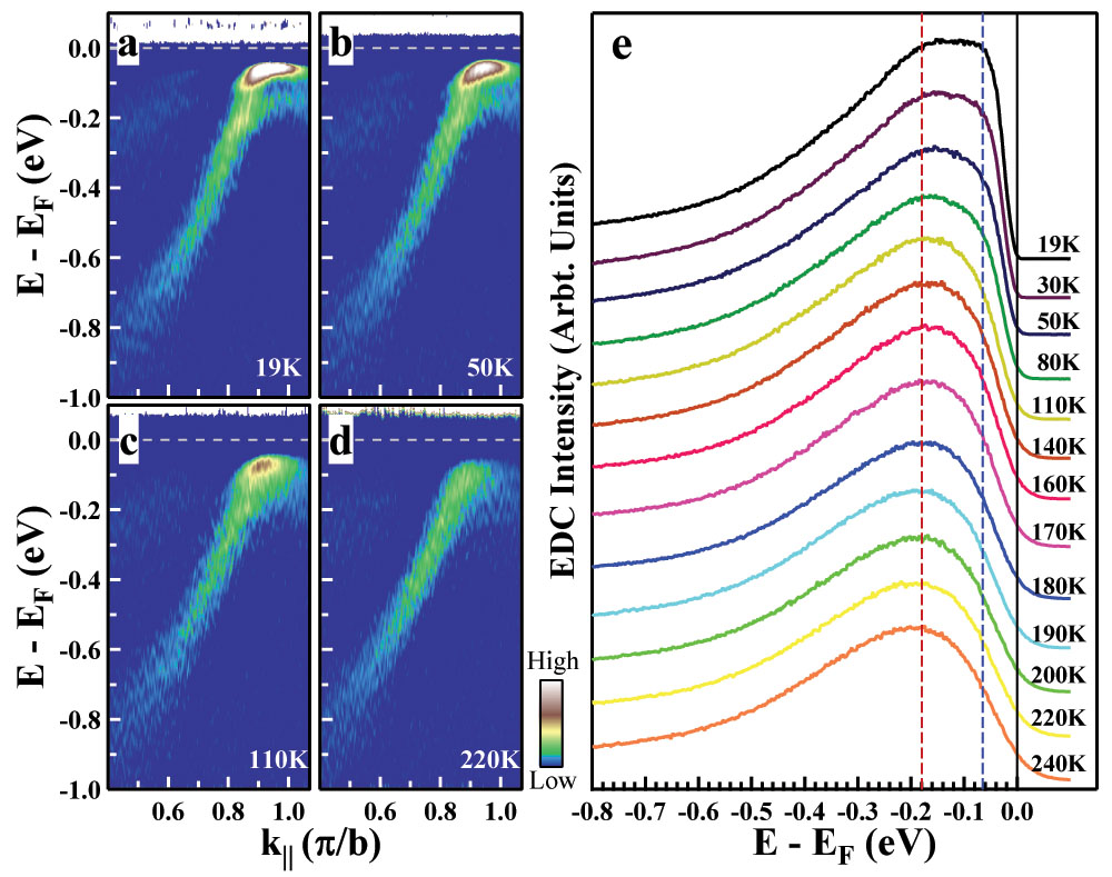
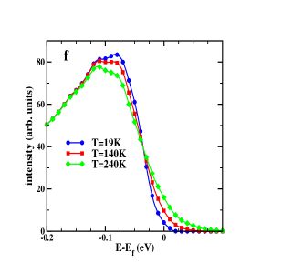
Figure 6: a) - d) EDC second derivative images of the B band along $\Gamma$-Y momentum cut at different temperatures. The data are divided by the Fermi-Dirac function. e) Extracted K_FB EDCs at different temperatures. Two energy scales of incoherent soliton and bound state are marked by blue and red dashed lines, respectively. f) The theoretical $K_{Fb}$ EDC’s for three different temperatures.

In this final section we present the temperature dependency of the asymmetry in the dispersion of spectral features to the left and to the right of $k=K_{FB}$. We present in Figs. 6, 7 the second derivative w.r.t. the energy of the photoemission spectra at four different temperatures, ranging from 19K to 240K, the final temperature being well above the CDW transition temperature, T${}_{c}=180$ K. We see the asymmetry in the dispersion is independent of temperature, persisting to well above $T_{c}$. However we also see that as the temperature is increased spectral features are blurred. The ability to distinguish between the contributions coming from the two branches (soliton/holon and bound state/holon) ceases at some temperature below T_c. This is to be expected. Sharp spectral features in correlated one dimensional systems see marked rounding even for temperatures a small fraction of the spectral gap finiteT .

While it is a difficult task to compute the thermal broadening in a strongly correlated electron system, the task is made easier if we focus on the holon/spinon contribution to the spectral function. We can then follow the strategy of Ref. finiteT . At least at low temperatures ($T\ll\Delta$), we can understand the spectral function’s thermal broadening by using the well understood form of the spectral contribution of the gapless holon (that of a Luttinger liquid at finite temperature Orgad ) while using the zero temperature form for the gapped spinon. While imperfect, this gives us a lower bound on the broadening of spectral lineshapes due to finite temperature. The results can be found in panel f of Fig. 1. We see that the broadening due to electronic correlations at finite temperature shares the same general features seen in the experiment (panel e of Fig. 1). There is an increase in spectral weight at energies, $E-E_{F}>0eV$ and a decrease in spectral weight at energies around $E-E_{F}\sim-0.15eV$. The increase in weight at $E-E_{F}>0eV$ seen theoretically as temperature is increased from 19K to 240K matches that seen experimentally. On the other hand the decrease in weight at $E-E_{F}\sim-0.15eV$ predicted theoretically by this calculation as temperature is increased underestimates that seen experimentally. While we again emphasize that our calculation only provides a lower bound on thermal broadening, it would certainly be reasonable (and expected) to need to ascribe some broadening to the presence of phonons.

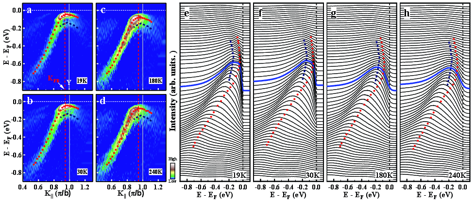
Figure 7: a)-d) The second derivative of high resolution measurements of the band structure along the $\Gamma-Y$ momentum cut with 1 meV energy resolution. Measurements for four different temperatures, below, at, and above the CDW transition temperature are shown. e)-h) The corresponding EDCs. The red circles and blue dashes mark the dispersion of the soliton/holon and the bound state/holon respectively.