Light baryons and their electromagnetic interactions
in the covariant constituent quark model

Abstract

We extend the confined covariant constituent quark model that was previously developed by us for mesons to the baryon sector. In our numerical calculation we use the same values for the constituent quark masses and the infrared cutoff as have been previously used in the meson sector. In a first application we describe the static properties of the proton and neutron, and the $\Lambda$-hyperon (magnetic moments and charge radii) and the behavior of the nucleon form factors at low momentum transfers. We discuss in some detail the conservation of gauge invariance of the electromagnetic transition matrix elements in the presence of a nonlocal coupling of the baryons to the three constituent quark fields.

I Introduction

We use the confined covariant constituent quark model (for short: covariant quark model) as dynamical input to calculate the electromagnetic transition matrix elements between light $(u,d,s)$ baryons. In the covariant quark model the current–induced transitions between baryons are calculated from two–loop Feynman diagrams with free quark propagators in which the high energy behavior of the loop integrations is tempered by Gaussian vertex functions Faessler:2001mr ; Faessler:2008ix ; Faessler:2009xn ; Branz:2010pq . An attractive new feature has recently been added to the covariant quark model inasmuch as quark confinement has now been incorporated in an effective way, i.e. there are no quark thresholds and thus no free quarks in the relevant Feynman diagrams Branz:2009cd ; Ivanov:2011aa . We emphasize that the covariant quark model described here is a truly frame–independent field theoretical quark model in contrast to other constituent quark models which are basically quantum mechanical with built–in relativistic elements.

In the covariant quark model we use the same values for the constituent quark masses and the infrared cutoff for all hadrons (mesons and baryons) independent of the hadron masses. We believe that the formulation of the confined covariant quark model constitutes a major advance both from the conceptual and the practical point of view. While an unconfined quark model is valid only for hadrons with masses low enough to lie below the sum of the constituent quark masses the confined covariant quark model can be applied to all hadrons regardless of their masses. The viability of the improved covariant quark model was demonstrated in a number of applications to mesonic transitions in Branz:2009cd . The form factors of the $B(B_{s})\to P(V)$ transitions were evaluated in Ivanov:2011aa , in a parameter-free way, in the full kinematical region of momentum transfer. As an application, the widths of some nonleptonic $B_{s}$ decays were also calculated. This approach was successfully applied to a study of the tetraquark state X(3872) and its strong and radiative decays (see, Refs. Dubnicka:2010kz ; Dubnicka:2011mm ).

In the present paper we formulate the covariant quark model with infrared confinement for the baryon sector. By keeping the same values for the constituent quark masses and the infrared cutoff as had been used in the meson sector we are able to reduce the number of free model parameters in the baryon sector to essentially the set of baryon size parameters. As a first application we describe the static properties of the nucleon and the $\Lambda$-baryon (magnetic moments and charge radii) and the behavior of the nucleon form factors at low momentum transfer. In a forthcoming publication next we are planning to study the rare decays of the $\Lambda_{b}$-baryon into the $\Lambda_{s}$ or the neutron. The present paper provides the necessary input for such a calculation in as much we determine the properties of the light baryons from their electromagnetic interactions.

The paper is structured as follows. In Sec. II we review the basic notions of our dynamical approach — the covariant quark model for baryons. We present the interaction Lagrangian describing the nonlocal coupling of a proton to its constituents, discuss the choice of interpolating currents and the vertex function, recall the compositeness condition for bound-state hadrons and show how the confinement ansatz is implemented in the baryon sector. In Sec. III we include the electromagnetic interactions of quarks and charged baryons in a manifestly gauge–invariant way, derive the Lagrangian describing the nonlocal interaction of the baryon, quark and electromagnetic fields. In Sec. IV we present the loop integration techniques that allow one to calculate the nucleon mass function and its derivative and the electromagnetic form factors of the nucleons. By analytically verifying the pertinent Ward and Ward–Takahashi identities we discuss in some detail how gauge invariance is maintained in the electromagnetic transitions. Sec. IV also contains our numerical results for the magnetic moments and form factors of the proton and neutron. We find that a particular superposition of vector and tensor interpolating currents gives satisfactory results for the nucleon static properties and form factors at low energies. In Sec. V we extend our approach to describe the static properties of the $\Lambda_{s}$ hyperon. We summarize our findings in Sec. VI.

II The covariant quark model for baryons

The basic ingredients of the covariant quark model for baryonic three quark states prior to the implementation of confinement can be found in Faessler:2001mr ; Faessler:2008ix ; Faessler:2009xn ; Branz:2010pq . This includes a description of the structure of the Gaussian vertex factor, the choice of interpolating baryon currents as well as the compositeness condition for baryons.

The new features introduced to the meson sector in Branz:2009cd ; Ivanov:2011aa and applied to the baryon sector in this paper are both technical and conceptual. Instead of using Feynman parameters for the evaluation of the two–loop baryonic quark model Feynman diagram we now use Schwinger parameters. The technical advantage is that this leads to a simplification of the tensor loop integrations inasmuch as the loop momenta occurring in the quark propagators can be written as derivative operators. Furthermore, the use of Schwinger parameters allows one to incorporate quark confinement in an effective way. Details of these two new features of the covariant quark model have been described in Branz:2009cd ; Ivanov:2011aa .

Let us enumerate the number of model parameters that are needed in our approach for the description of baryons. As stated in the introduction the values of the constituent quark masses and the universal confinement parameter are taken over from the meson sector. The coupling strength of a baryon to its constituent quarks is fixed by the compositeness condition. This leaves one with one size parameter for each baryon. For the present paper we need the size parameters of the proton, neutron and $\Lambda_{s}$. Naturally we use the same size parameter for the proton and the neutron. The size parameters are determined by a fit to the static e.m. properties and form factors of the nucleons and the $\Lambda_{s}$. We have added one more parameter to the set of basic parameters which describes the mixing between vector and tensor interpolating currents.

II.1 Lagrangian and three-quark currents

Let us begin our discussion with the proton. The coupling of a proton to its constituent quarks is described by the Lagrangian

$${\cal L}^{\,\rm p}_{\rm int}(x)=g_{N}\,\bar{p}(x)\cdot J_{p}(x)+g_{N}\,\bar{J}_{p}(x)\cdot p(x)\,,$$ (1)

where we make use of the same interpolating three-quark current $J_{p}(\bar{J}_{p})$ as in Ref. Ivanov:1996pz

$$J_{p}(x) = \int\!\!dx_{1}\!\!\int\!\!dx_{2}\!\!\int\!\!dx_{3}\,F_{N}(x;x_{1},x_{2},x_{3})\,J^{(p)}_{3q}(x_{1},x_{2},x_{3})\,,$$

$$J^{(p)}_{3q}(x_{1},x_{2},x_{3}) = \Gamma^{A}\gamma^{5}\,d^{a_{1}}(x_{1})\cdot[\epsilon^{a_{1}a_{2}a_{3}}\,u^{a_{2}}(x_{2})\,C\,\Gamma_{A}\,u^{a_{3}}(x_{3})]\,,$$

$$\bar{J}_{p}(x) = \int\!\!dx_{1}\!\!\int\!\!dx_{2}\!\!\int\!\!dx_{3}\,F_{N}(x;x_{1},x_{2},x_{3})\,\bar{J}^{(p)}_{3q}(x_{1},x_{2},x_{3})\,,$$

$$\bar{J}^{(p)}_{3q}(x_{1},x_{2},x_{3}) = [\epsilon^{a_{1}a_{2}a_{3}}\,\bar{u}^{a_{3}}(x_{3})\,\Gamma_{A}\,C\,\bar{u}^{a_{2}}(x_{2})]\cdot\bar{d}^{a_{1}}(x_{1})\gamma^{5}\Gamma^{A}\,.$$

The matrix $C=\gamma^{0}\gamma^{2}$ is the usual charge conjugation matrix and the $a_{i}$ $(i=1,2,3)$ are color indices. There are two possible kinds of nonderivative three-quark currents: $\Gamma^{A}\otimes\Gamma_{A}=\gamma^{\alpha}\otimes\gamma_{\alpha}$ (vector current) and $\Gamma^{A}\otimes\Gamma_{A}=\frac{1}{2}\,\sigma^{\alpha\beta}\otimes\sigma_{\alpha\beta}$ (tensor current) with $\sigma^{\alpha\beta}=\tfrac{i}{2}(\gamma^{\alpha}\gamma^{\beta}-\gamma^{\beta}\gamma^{\alpha}).$ The interpolating current of the neutron and the corresponding Lagrangian are obtained from the proton case via $p\to n$ and $u\leftrightarrow d$. As will become apparent later on, one has to consider a general linear superposition of the vector and tensor currents according to

$$J_{N}=xJ^{T}_{N}+(1-x)J^{V}_{N}\,,\quad N=p,n$$ (3)

where the mixing parameter $x$ extends from zero to one  ($0\leq x\leq 1$). When taking the nonrelativistic limit of the vector and tensor currents one finds that the two currents become degenerate. The limiting currents for the proton and the neutron read

$$J^{T}_{p}\equiv J^{V}_{p}\ =\ \epsilon^{a_{1}a_{2}a_{3}}\ \vec{\sigma}\,\psi_{d}^{a_{1}}\ (\psi_{u}^{a_{2}}\,\sigma_{2}\vec{\sigma}\,\psi_{u}^{a_{3}})\,,\qquad J^{T}_{n}\equiv J^{V}_{n}\ =\ \epsilon^{a_{1}a_{2}a_{3}}\ \vec{\sigma}\,\psi_{u}^{a_{1}}\ (\psi_{d}^{a_{2}}\,\sigma_{2}\vec{\sigma}\,\psi_{d}^{a_{3}})\,,$$ (4)

where $\psi_{u,d}$ are the upper components of the respective Dirac quark spinor fields and where $\sigma_{i}$ are Pauli spin matrices.

Most of the properties of the nucleons are only weakly dependent on the choice of interpolating currents. However, in order to get the correct value for the charge radius of the neutron, one needs to use the superposition of currents Eq. (3) even though the currents $J^{T}$ and $J^{V}$ become degenerate in the nonrelativistic limit. In view of the fact that a nonrelativistic description of the neutron gives zero values for the charge radius of the neutron deAraujo:2003ke this is an indication that relativistic corrections play a crucial role for the desciption of the neutron charge radius.

The vertex function $F_{N}$ characterizes the finite size of the nucleon. We assume that the vertex function is real and the same for the proton and the neutron. To satisfy translational invariance the function $F_{N}$ has to satisfy the identity

$$F_{N}(x+a;x_{1}+a,x_{2}+a,x_{3}+a)\,=\,F_{N}(x;x_{1},x_{2},x_{3})$$ (5)

for any given 4-vector $a\,$. We use the following representation for the vertex function

$$F_{N}(x;x_{1},x_{2},x_{3})\,=\,\delta^{(4)}(x-\sum\limits_{i=1}^{3}w_{i}x_{i})\;\Phi_{N}\biggl{(}\sum_{i<j}(x_{i}-x_{j})^{2}\biggr{)}\,,$$ (6)

where $\Phi_{N}$ is the correlation function of the three constituent quarks with the coordinates $x_{1}$, $x_{2}$, $x_{3}$ and masses $m_{1}$, $m_{2}$, $m_{3}$, respectively. The variable $w_{i}$ is defined by $w_{i}=m_{i}/(m_{1}+m_{2}+m_{3})$ such that $\sum_{i=1}^{3}w_{i}=1$. Note that $F_{N}(x;x_{1},x_{2},x_{3})$ is symmetric in the coordinates $x_{i}$, i.e. symmetric under $x_{i}\leftrightarrow{x_{j}}$.

We shall make use of the Jacobi coordinates $\rho_{1,2}$ and the CM coordinate $x$ which are defined by

$$x_{1} = x\,+\,\tfrac{1}{\sqrt{2}}\,w_{3}\,\rho_{1}\,-\,\tfrac{1}{\sqrt{6}}\,(2w_{2}+w_{3})\,\rho_{2}\,,$$

$$x_{2} = x\,+\,\tfrac{1}{\sqrt{2}}\,w_{3}\,\rho_{1}\,+\,\tfrac{1}{\sqrt{6}}\,(2w_{1}+w_{3})\,\rho_{2}\,,$$

$$x_{3} = x\,-\,\tfrac{1}{\sqrt{2}}\,(w_{1}+w_{2})\,\rho_{1}\,+\,\tfrac{1}{\sqrt{6}}\,(w_{1}-w_{2})\,\rho_{2}\,.$$ (7)

The CM coordinate is given by $x\,=\,\sum_{i=1}^{3}w_{i}x_{i}$. In terms of the Jacobi coordinates one obtains

$$\sum\limits_{i<j}(x_{i}-x_{j})^{2}=\rho_{1}^{2}+\rho_{2}^{2}\,.$$ (8)

Note that the choice of Jacobi coordinates is not unique. With the above choice Eq. (7) one readily arrives at the following representation for the correlation function $\Phi_{N}$ in Eq. (6)

$$\Phi_{N}\biggl{(}\sum_{i<j}(x_{i}-x_{j})^{2}\biggr{)} = \int\!\frac{d^{4}p_{1}}{(2\pi)^{4}}\!\int\!\frac{d^{4}p_{2}}{(2\pi)^{4}}\,e^{-ip_{1}(x_{1}-x_{3})-ip_{2}(x_{2}-x_{3})}\,\bar{\Phi}_{N}(-P^{2}_{1}-P^{2}_{2})\,,$$ (9)

$$\bar{\Phi}_{N}(-P^{2}_{1}-P^{2}_{2}) = \tfrac{1}{9}\int\!d^{4}\rho_{1}\int\!d^{4}\rho_{2}\,e^{iP_{1}\rho_{1}+iP_{2}\rho_{2}}\,\Phi_{N}(\rho^{2}_{1}+\rho^{2}_{2})\,,$$

$$P_{1}=\tfrac{1}{\sqrt{2}}(p_{1}+p_{2})\,,\qquad P_{2}=-\tfrac{1}{\sqrt{6}}(p_{1}-p_{2})\,.$$

Even if the above choice of Jacobi coordinates was used to derive (9) the representation (9) in its general form can be seen to be valid for any choice of Jacobi coordinates. The particular choice (7) is a preferred choice since it leads to the specific form of the argument $-P^{2}_{1}-P^{2}_{2}=-\tfrac{2}{3}(p_{1}^{2}+p_{2}^{2}+p_{1}p_{2})$. Since this expression is invariant under the transformations: $p_{1}\leftrightarrow p_{2}$, $p_{2}\to-p_{2}-p_{1}$ and $p_{1}\to-p_{1}-p_{2}$, the r.h.s. in Eq. (9) is invariant under permutations of all $x_{i}$ as it should be.

In the next step we have to specify the function $\bar{\Phi}_{N}(-P^{2}_{1}-P^{2}_{2})\equiv\bar{\Phi}_{N}(-P^{2})$, which characterizes the finite size of the baryons. We will choose a simple Gaussian form for the function $\bar{\Phi}_{N}$

$$\bar{\Phi}_{N}(-P^{2})=\exp(P^{\,2}/\Lambda_{N}^{2})\,,$$ (10)

where $\Lambda_{N}$ is a size parameter parametrizing the distribution of quarks inside a nucleon. Note that we have used another definition of the $\Lambda_{N}$ in our previous papers: $\Lambda_{N}=\Lambda_{N}^{\rm old}/(3\sqrt{2}).$

Since $P^{\,2}$ turns into $-\,P^{\,2}_{E}$ in Euclidean space the form (10) has the appropriate fall–off behavior in the Euclidean region. We emphasize that any choice for $\Phi_{N}$ is appropriate as long as it falls off sufficiently fast in the ultraviolet region of Euclidean space to render the corresponding Feynman diagrams ultraviolet finite. The choice of a Gaussian form for $\Phi_{H}$ has obvious calculational advantages.

The coupling constants $g_{N}$ are determined by the compositeness condition suggested by Weinberg Weinberg:1962hj and Salam Salam:1962ap (for a review, see Hayashi:1967hk ) and extensively used by us in previous papers on the covariant quark model (for details, see Efimov:1993ei ). The compositeness condition postulates that the renormalization constant of the bound-state wave function is set equal to zero. In the case of a baryon this implies that

$$Z_{N}=1-\Sigma^{\prime}_{N}(m_{N})=0\,,$$ (11)

where $\Sigma^{\prime}_{N}$ is the on-shell derivative of the nucleon mass function $\Sigma_{N}$, i.e. $\Sigma^{\prime}_{N}=\partial\,\Sigma_{N}/\partial\!\!\not\!p$, at $p^{2}=m_{N}^{2}$ and where $m_{N}$ is the nucleon mass. The compositeness condition is the central equation of our covariant quark model. It can be viewed as the field theoretic equivalent of the wave function normalization condition for quantum mechanical wave functions. The physical meaning, the implications and corollaries of the compositeness condition have been discussed in some detail in our previous papers (see e.g. Branz:2009cd ).

II.2 Infrared confinement

In Branz:2009cd we have shown how the confinement of quarks can be effectively incorporated in the covariant quark model. In a first step, we introduced an additional scale integration in the space of Schwinger’s $\alpha$–parameters with an integration range from zero to infinity. In a second step the scale integration was cut off at the upper limit which corresponds to the introduction of an infrared (IR) cutoff. In this manner all possible thresholds present in the initial quark diagram were removed. The cutoff parameter was taken to be the same for all physical processes. Other model parameters such as the constituent quark masses and size parameters were determined from a fit to experimental data.

Let us describe the basic features of how IR confinement is implemented in our model. All physical matrix elements are described by Feynman diagrams written in terms of a convolution of free quark propagators and the vertex functions. Let $n$ and $m$ be the number of the propagators and vertices, respectively. For the current-induced baryon transitions or the derivative of the mass function one has four quark propagators and two vertex functions, i.e. one has $n=4$ and $m=2$. In Minkowski space the two-loop diagram will be represented as

$$\Pi(p_{1},...,p_{m}) = \int\!\![d^{4}k]^{2}\prod\limits_{i_{1}=1}^{m}\,\Phi_{i_{1}+n}\left(-K^{2}_{i_{1}+n}\right)\prod\limits_{i_{3}=1}^{n}\,S_{i_{3}}(\tilde{k}_{i_{3}}+v_{i_{3}}),$$

$$K^{2}_{i_{1}+n} = \sum_{i_{2}}(\tilde{k}^{(i_{2})}_{i_{1}+n}+v^{(i_{2})}_{i_{1}+n})^{2}\,,$$ (12)

where the vectors $\tilde{k}_{i}$ are linear combinations of the loop momenta $k_{i}$. The $v_{i}$ are linear combinations of the external momenta $p_{i}$. The strings of Dirac matrices appearing in the calculation need not concern us here since they do not depend on the momenta. The external momenta $p_{i}$ are all chosen to be ingoing such that one has $\sum\limits_{i=1}^{m}p_{i}=0$.

Using the Schwinger representation the local quark propagator is written as

$$S(k)=\frac{1}{m-\not\!k}=(m+\not\!k)\int\limits_{0}^{\infty}\!d\beta\,e^{-\beta\,(m^{2}-k^{2})}\,.$$ (13)

As mentioned before one takes the Gaussian form or the vertex functions, i.e.

$$\bar{\Phi}_{i+n}\left(-K^{2}\right)\,=\exp\left[\beta_{i+n}\,K^{2}\right]\qquad i=1,...,m\,,$$ (14)

where, as in (10), the parameters $\beta_{i+n}$ are related to the respective size parameters of the baryons $\Lambda_{i}$ via $\beta_{i+n}=1/\Lambda^{2}_{i}$. The integrand in Eq. (12) has a Gaussian form with the exponential factor $(kak+2kr+R)$ where, in case of the baryonic two-loop calculation, $a$ is a $2\times 2$ matrix depending on the parameters $\beta_{i}$, $r$ is a $2$-component vector composed from the external momenta, $k$ is a $2$-component vector of the loop momenta of the form $k=(k_{1},k_{2})$ and $R$ is a quadratic form of the external momenta. Tensor loop integrals are calculated with the help of the differential representation

$$k_{i}^{\mu}e^{2kr}=\frac{1}{2}\frac{\partial}{\partial r_{i\,\mu}}e^{2kr}\,.$$ (15)

After doing the loop integration the differential operators $\partial/\partial r_{i\,\mu}$ will give cause to outer momenta tensors which, in the present case, are $p$ and $p^{\prime}$. We have written a FORM Vermaseren:2000nd program that achieves the necessary commutations of the differential operators in a very efficient way.

After doing the loop integrations one obtains ($n$ denotes the number of propagators)

$$\Pi=\int\limits_{0}^{\infty}d^{n}\beta\,F(\beta_{1},\ldots,\beta_{n})\,,$$ (16)

where $F$ stands for the whole structure of a given diagram. The set of Schwinger parameters $\beta_{i}$ can be turned into a simplex by introducing an additional $t$–integration via the identity

$$1=\int\limits_{0}^{\infty}dt\,\delta(t-\sum\limits_{i=1}^{n}\beta_{i})$$ (17)

leading to

$$\Pi=\int\limits_{0}^{\infty}\!dtt^{n-1}\!\!\int\limits_{0}^{1}\!d^{n}\alpha\,\delta\Big{(}1-\sum\limits_{i=1}^{n}\alpha_{i}\Big{)}\,F(t\alpha_{1},\ldots,t\alpha_{n}).$$ (18)

There are altogether $n$ numerical integrations: $(n-1)$ $\alpha$–parameter integrations and the integration over the scale parameter $t$. The very large $t$–region corresponds to the region where the singularities of the diagram with its local quark propagators start appearing. However, as described in Branz:2009cd , if one introduces an IR cutoff on the upper limit of the $t$–integration, all singularities vanish because the integral is now analytic for any value of the set of kinematic variables. We cut off the upper integration at $1/\lambda^{2}$ and obtain

$$\Pi^{c}=\!\!\int\limits_{0}^{1/\lambda^{2}}\!\!dtt^{n-1}\!\!\int\limits_{0}^{1}\!d^{n}\alpha\,\delta\Big{(}1-\sum\limits_{i=1}^{n}\alpha_{i}\Big{)}\,F(t\alpha_{1},\ldots,t\alpha_{n}).$$ (19)

By introducing the IR cutoff one has removed all potential thresholds in the quark loop diagram, i.e. the quarks are never on-shell and are thus effectively confined. We mention that an explicit demonstration of the absence of a two- quark threshold in the case of a scalar one–loop two–point function has been given in Ref. Branz:2009cd . We take the infrared cutoff parameter $\lambda$ to be the same in all physical processes. The numerical evaluations have been done by a numerical program written in the FORTRAN code.

III Electromagnetic interactions

We use the standard free fermion Lagrangian for the baryon and quark fields:

$${\cal L}_{\rm free}(x)=\bar{B}(x)(i\not\!\partial-m_{B})B(x)+\sum\limits_{q}\,\bar{q}(x)(i\not\!\partial-m_{q})q(x)\,,$$ (20)

where $m_{q}$ is the constituent quark mass. The interaction with the electromagnetic field has to be introduced both at the baryon and the quark level. In a first step we gauge the free Lagrangians Eq. (20) of the quark and baryon fields in the standard manner by using minimal substitution:

$$\partial^{\mu}B\to(\partial^{\mu}-ie_{B}A^{\mu})B\,,\qquad\partial^{\mu}q_{i}\to(\partial^{\mu}-ie_{q_{i}}A^{\mu})q_{i}\,,$$ (21)

where $e_{B}$ is the electric charge of the baryon $B$ and $e_{q_{i}}$ is the electric charge of the quark with flavor $q_{i}$. The interaction of the baryon and quark fields with the e.m. field is thus specified by minimal substitution. The interaction Lagrangian reads

$${\cal L}^{\rm em-min}_{\rm int}(x)=e_{B}\bar{B}(x)\!\not\!\!A\,B(x)+\sum\limits_{q}\,e_{q}\,\bar{q}(x)\!\not\!\!A\,q(x)\,.$$ (22)

As will become apparent further on, the electromagnetic field does not directly couple to the baryon fields as a result of the compositeness condition.

Next one gauges the nonlocal Lagrangian Eq. (1). The gauging proceeds in a way suggested in Refs. Mandelstam:1962mi ; Terning:1991yt and used before by us (see, for instance, Refs.  Ivanov:1996pz ; Faessler:2006ft ). In order to guarantee local invariance of the strong interaction Lagrangian one multiplies each quark field $q(x_{i})$ in ${\cal L}_{\rm int}^{\rm str}$ with a gauge field exponential. One then has

$$q_{i}(x_{i})\to e^{-ie_{q_{1}}I(x_{i},x,P)}\,q_{i}(x_{i})\,,$$ (23)

where

$$I(x_{i},x,P)=\int\limits_{x}^{x_{i}}dz_{\mu}A^{\mu}(z).$$ (24)

The path $P$ connects the end-points of the path integral.

It is readily seen that the full Lagrangian is invariant under the transformations

$$\begin{aligned} &q_{i}(x)\,\to\,e^{ie_{q_{i}}f(x)}q_{i}(x)\,,\qquad\bar{q}_{i}(x)\,\to\,\bar{q}_{i}(x)\,e^{-ie_{q_{i}}f(x)}\,,\\ &B(x)\,\to\,e^{ie_{B}f(x)}\,B(x)\,,\qquad\bar{B}(x)\,\to\,\bar{B}(x)\,e^{-ie_{B}f(x)}\,,\\ &A^{\mu}(x)\,\to\,A^{\mu}(x)+\partial^{\mu}f(x)\,,\end{aligned}$$

where $e_{B}=\sum\limits_{i=1}^{3}e_{q_{i}}$.

One then expands the gauge exponential up to the requisite power of $e_{q}A_{\mu}$ needed in the perturbative series. This will give rise to a second term in the nonlocal electromagnetic interaction Lagrangian ${\cal L}^{\rm em-nonloc}_{\rm int}$. Superficially it appears that the results will depend on the path $P$ taken to connect the end-points in the path integral in Eq. (24). However, one needs to know only the derivatives of the path integral expressions when calculating the perturbative series. Therefore, we use the formalism suggested in Mandelstam:1962mi ; Terning:1991yt which is based on the path-independent definition of the derivative of $I(x,y,P)$:

$$\lim\limits_{dx^{\mu}\to 0}dx^{\mu}\frac{\partial}{\partial x^{\mu}}I(x,y,P)\,=\,\lim\limits_{dx^{\mu}\to 0}[I(x+dx,y,P^{\prime})-I(x,y,P)]$$ (25)

where the path $P^{\prime}$ is obtained from $P$ by shifting the end-point $x$ by $dx$. The definition (25) leads to the key rule

$$\frac{\partial}{\partial x^{\mu}}I(x,y,P)=A_{\mu}(x)$$ (26)

which in turn states that the derivative of the path integral $I(x,y,P)$ does not depend on the path $P$ originally used in the definition.

As a result of this rule the Lagrangian describing the nonlocal interaction of the baryon, quark and electromagnetic fields to the first order in the electromagnetic charge reads

$${\cal L}^{\,\rm em-nonloc}_{\rm int}(x)=g_{B}\,\bar{B}(x)\cdot\!\!\int\!\!dyA_{\alpha}(y)J_{B-\rm em}^{\alpha}(x,y)+g_{B}\int\!\!dyA_{\alpha}(y)\bar{J}_{B-\rm em}^{\alpha}(x,y)\cdot B(x)\,,$$ (27)

where the nonlocal electromagnetic currents are given by

$$J_{B-\rm em}^{\alpha}\,(x,y) = \prod\limits_{i=1}^{3}\int\!\!dx_{i}\,J^{(B)}_{3q}(x_{1},x_{2},x_{3})\,E^{\alpha}_{B}(x;x_{1},x_{2},x_{3};y)\,,$$

$$\bar{J}_{B-\rm em}^{\alpha}(x,y) = \prod\limits_{i=1}^{3}\int\!\!dx_{i}\,\bar{J}^{(B)}_{3q}(x_{1},x_{2},x_{3})\,E^{\alpha\,\dagger}_{B}(x;x_{1},x_{2},x_{3};y)\,,$$

$$E^{\alpha}_{B}(x;x_{1},x_{2},x_{3};y) = \prod\limits_{i=1}^{3}\int\!\!\frac{dp_{i}}{(2\pi)^{4}}\!\!\int\!\!\frac{dr}{(2\pi)^{4}}\,e^{-i\sum\limits_{i=1}^{3}p_{i}(x-x_{i})-ir(x-y)}\,\widetilde{E}^{\alpha}_{B}(p_{1},p_{2},p_{3};r)\,,$$

$$\widetilde{E}^{\alpha}_{B}(p_{1},p_{2},p_{3};r) = \sum\limits_{i=1}^{3}e_{q_{i}}\int\limits_{0}^{1}d\tau\Big{\{}-w_{i1}(w_{i1}r^{\alpha}+2q_{1}^{\alpha})\bar{\Phi}^{\prime}_{B}(-z_{1})-w_{i2}(w_{i2}r^{\alpha}+2q_{2}^{\alpha})\bar{\Phi}^{\prime}_{B}(-z_{2})\Big{\}}\,,$$ (28)

Further

$$q_{1} = \sum\limits_{i=1}^{3}w_{i1}p_{i}\,,\qquad q_{2}=\sum\limits_{i=1}^{3}w_{i2}p_{i}\,,$$

$$z_{1} = \tau(w_{i1}r+q_{1})^{2}-(1-\tau)q_{1}^{2}-(w_{i2}r+q_{2})^{2}\,,\qquad z_{2}=q_{1}^{2}-\tau(w_{i2}r+q_{2})^{2}-(1-\tau)q_{2}^{2}\,,$$

$$w_{i1} = \left(\begin{array}[]{c}\tfrac{1}{\sqrt{2}}w_{3}\\ \tfrac{1}{\sqrt{2}}w_{3}\\ -\tfrac{1}{\sqrt{2}}(w_{1}+w_{2})\end{array}\right)\,,\qquad w_{i2}=\left(\begin{array}[]{c}-\tfrac{1}{\sqrt{6}}(2w_{2}+w_{3})\\ \tfrac{1}{\sqrt{6}}(2w_{1}+w_{3})\\ \tfrac{1}{\sqrt{6}}(w_{1}-w_{2})\end{array}\right)\,.$$ (35)

IV Nucleon mass function and electromagnetic form factors

We start with the calculation of the proton mass function (also called self-energy function) needed for the implementation of the compositeness condition. The relevant term in the expansion of the $S$–matrix reads

$$S_{2} = i^{2}g_{N}^{2}\int\!\!dx\!\!\int\!\!dy\,\bar{p}(x)\langle 0|T\{J_{p}(x)\bar{J}_{p}(y)\}|0\rangle p(y)\,$$ (36)

$$\doteq i\int\!\!dx\!\!\int\!\!dy\,\bar{p}(x)\Sigma_{p}(x-y)p(y)\,.$$

The corresponding two–loop Feynman quark diagram is shown in Fig. 1. In Eq. (36) we have introduced the standard notation for the proton mass function

$$\Sigma_{p}(x-y)=ig_{N}^{2}\,\langle 0|T\{J_{p}(x)\bar{J}_{p}(y)\}|0\rangle\,.$$ (37)

The Fourier-transform of the mass function $\Sigma_{p}(x-y)$ is given by

$$\Sigma_{p}(x-y)=\int\!\!\frac{d^{4}p}{(2\pi)^{4}}\,e^{-ip(x-y)}\,\Sigma_{p}(p)\,,\qquad\Sigma_{p}(p)=\int\!\!d^{4}x\,e^{ipx}\Sigma_{p}(x)\,.$$ (38)

We use the same notation $\Sigma_{p}$ for the mass function of the proton in coordinate space and in momentum space. Which of the two representations are being used can be read off from the arguments, cif. $\Sigma_{p}(x-y)$ and $\Sigma_{p}(p)$. The matrix element of $S_{2}$ in Eq. (36) between the initial and final proton states (with momenta $p$ and $p^{\prime}$, respectively) is expressed by

$$\langle p^{\prime}|S_{2}|p\rangle\,=\,i\,(2\pi)^{4}\,\delta^{(4)}(p-p^{\prime})\,\bar{u}_{p}(p)\,\Sigma_{p}(p)\,u_{p}(p)\,.$$ (39)

It is straightforward but nevertheless cumbersome to calculate the proton mass function $\Sigma_{p}(x-y)$. One uses the explicit expression for the interpolating three–quark current given by Eq. (LABEL:eq:current) and the time–ordering of quark fields:

$$\langle 0|T\{\,q^{a}_{f}(x)\bar{q}^{\,a^{\prime}}_{f^{\prime}}(y)\,\}|0\rangle=\delta_{aa^{\prime}}\delta_{ff^{\prime}}\,S_{f}(x-y)=\delta_{aa^{\prime}}\delta_{ff^{\prime}}\int\!\!\frac{d^{4}k}{(2\pi)^{4}i}\,e^{-ik(x-y)}\,S_{f}(k)\,,$$ (40)

where $S_{f}(x-y)$ and $S_{f}(k)$ are the free quark propagators in coordinate and momentum space with

$$S_{f}(k)=\frac{1}{m_{f}-\not\!k}\,$$ (41)

and where $a,a^{\prime}$ and $f,f^{\prime}$ are color and flavor indices, respectively.

In momentum space the proton mass function is given by

$$\Sigma_{p}(p)=12g_{N}^{2}\,\int\!\!\frac{d^{4}k_{1}}{(2\pi)^{4}i}\!\!\int\!\!\frac{d^{4}k_{2}}{(2\pi)^{4}i}\bar{\Phi}_{N}^{2}(-z_{0})\Gamma^{A}\gamma^{5}S_{d}(k_{1}+w_{1}p)\gamma^{5}\Gamma^{B}\mbox{\rm{tr}}\left[S_{u}(k_{2}-w_{2}p)\Gamma_{A}S_{u}(k_{2}-k_{1}+w_{3}p)\Gamma_{B}\right]\,,$$ (42)

where

$$z_{0}=\tfrac{1}{2}(k_{1}-k_{2})^{2}+\tfrac{1}{6}(k_{1}+k_{2})^{2}\,.$$ (43)

In order to economize on the notation we introduce a short-hand notation for the two loop momentum integrations in (42) and in the following formulas. We write

$$\langle\langle\ldots\rangle\rangle=\int\!\!\frac{d^{4}k_{1}}{(2\pi)^{4}i}\!\!\int\!\!\frac{d^{4}k_{2}}{(2\pi)^{4}i}\,(\ldots)\,\,.$$ (44)

Note that the integral Eq. (42) is invariant under a shift of the loop momenta $k_{i}\to k_{i}+ap$ where $a$ is an arbitrary number and $p$ is the outer momentum. Using this invariance one can obtain various equivalent representations for the mass function. In Eq. (42) we have chosen $a$ such that the external momentum does not appear in the argument of the vertex function. One has $w_{2}=w_{3}=\tfrac{1}{2}(1-w_{1})$ where $w_{1}=m_{d}/(m_{d}+2m_{u})$. We mention that it is convenient to keep $m_{u}\neq m_{d}$ in the analytical calculation in order to distinguish the proton from the neutron case. In the end, when we do the numerical calculation, we set $m_{u}=m_{d}$.

According to the compositeness condition Eq. (11) one needs to calculate the derivative of the proton mass function. Since the proton is on mass–shell, i.e. $\bar{u}(p)\!\!\!\not\!\!p\,u(p)=m_{N}\bar{u}(p)u(p)$ and hence $p^{\mu}\bar{u}(p)u(p)=m_{N}\bar{u}(p)\gamma^{\mu}u(p)$, the compositeness condition

$$\Sigma_{p}^{\prime}(p)=\frac{\partial\Sigma_{p}(p)}{\partial\!\!\not\!p}\,=\,1\quad\text{with}\quad\not\!p=m_{N}$$ (45)

can be written as

$$\frac{\partial\Sigma_{p}(p)}{\partial p_{\mu}}\,=\,\gamma^{\mu}\quad\text{with}\quad\not\!p=m_{N}\quad\text{and}\quad p^{\mu}=m_{N}\gamma^{\mu}\,.$$ (46)

Here and in the following it is understood that the relations between Green functions are valid when sandwiched between spinors. The latter form (46) is more suitable for our calculation because of its relation to the electromagnetic proton vertex function at zero momentum transfer. Using

$$\frac{\partial}{\partial p_{\mu}}S_{f}(k+wp)=w\,S_{f}(k+wp)\gamma^{\mu}S_{f}(k+wp)$$ (47)

one obtains

$$\frac{\partial\Sigma_{p}(p)}{\partial p_{\mu}} = 12g_{N}^{2}{\Big{\langle}\Big{\langle}}\bar{\Phi}_{N}^{2}(-z_{0})\Big{\{}w_{1}\Gamma^{A}\gamma^{5}S_{d}(k_{1}+w_{1}p)\gamma^{\mu}S_{d}(k_{1}+w_{1}p)\gamma^{5}\Gamma^{B}\mbox{\rm{tr}}\left[S_{u}(k_{2}-w_{2}p)\Gamma_{A}S_{u}(k_{2}-k_{1}+w_{3}p)\Gamma_{B}\right]$$ (48)

$$-\,w_{2}\Gamma^{A}\gamma^{5}S_{d}(k_{1}+w_{1}p)\gamma^{5}\Gamma^{B}\mbox{\rm{tr}}\left[S_{u}(k_{2}-w_{2}p)\gamma^{\mu}S_{u}(k_{2}-w_{2}p)\Gamma_{A}S_{u}(k_{2}-k_{1}+w_{3}p)\Gamma_{B}\right]$$

$$+\,w_{3}\Gamma^{A}\gamma^{5}S_{d}(k_{1}+w_{1}p)\gamma^{5}\Gamma^{B}\mbox{\rm{tr}}\left[S_{u}(k_{2}-w_{2}p)\Gamma_{A}S_{u}(k_{2}-k_{1}+w_{3}p)\gamma^{\mu}S_{u}(k_{2}-k_{1}+w_{3}p)\Gamma_{B}\right]\Big{\}}\Big{\rangle}\Big{\rangle}\,.$$

We now return to the calculation of the electromagnetic vertex of the proton. There are two terms in the relevant expansion of the $S$-matrix. These are derived i) from the Lagrangian Eq. (22) describing the local interaction of the photon with the quarks and ii) from the Lagrangian Eq. (27) describing the nonlocal interaction nucleon+quarks+photon. One has

$$S_{3} = i^{3}g_{N}^{2}\int\!\!dx\!\!\int\!\!dy\!\!\int\!\!dz\,A_{\mu}(z)\,\bar{p}(x)\langle 0|T\{J_{p}(x)\,\left(e_{u}\,\bar{u}(z)\gamma^{\mu}u(z)+e_{d}\,\bar{d}(z)\gamma^{\mu}d(z)\right)\bar{J}_{p}(y)\}|0\rangle p(y)$$ (49)

$$+ i^{2}g_{N}^{2}\int\!\!dx\!\!\int\!\!dy\!\!\int\!\!dz\,A_{\mu}(z)\,\bar{p}(x)\langle 0|T\{J_{p}(x)\,\bar{J}_{p-\rm em}^{\mu}(y,z)+J_{p-\rm em}^{\mu}(x,z)\bar{J}_{p}(y)\}|0\rangle p(y)\,,$$

where the currents $J_{p}(\bar{J}_{p})$ and $J_{p-\rm em}^{\mu}(\bar{J}_{p-\rm em}^{\mu})$ are defined by Eqs. (LABEL:eq:current) and (28), respectively. It is important to keep track of the signs of the various charges in the calculation. Our choice is to take the electric charges of charged particles in units of the proton charge, e.g. $e_{p}=+1$, $e_{u}=+2/3$, $e_{d}=-1/3$, etc.

The matrix element $S_{3}$ in Eq. (49) taken between the initial and final proton states with momenta ($p$) and ($p^{\prime}$) and the photon state with momentum ($q=p-p^{\prime}$) reads

$$\langle p^{\prime};q,\mu|S_{3}|p\rangle\,=\,\bar{u}_{p}(p^{\prime})\,T_{3}^{\mu}(p;p^{\prime},q)\,u_{p}(p)\,.$$ (50)

The matrix element $T^{\mu}_{3}(p;p^{\prime}q)$ is obtained from Eq. (49) by the substitutions $A_{\mu}(z)\to e^{iqz}$, $\bar{p}(x)\to e^{ip^{\prime}x}$ and $p(y)\to e^{-ipy}$. A straightforward calculation gives

$$T_{3}^{\mu}(p;p^{\prime},q)=i(2\pi)^{4}\delta^{(4)}(p-p^{\prime}-q)\Lambda_{p}^{\mu}(p,p^{\prime})\,$$ (51)

where the electromagnetic vertex function $\Lambda_{p}^{\mu}(p,p^{\prime})$ of the proton consists of four pieces represented by the four two-loop quark diagrams in Fig.2:

• the vertex diagram with the e.m. current attached to the d-quark (Fig.2a)  — $\Lambda^{\mu}_{p\,\rm d}$,

• the vertex diagram with the e.m. current attached to the u-quark (Fig.2b)  — $\Lambda^{\mu}_{p\,\rm u}$,

• two bubble diagrams with the e.m. current attached to the initial proton vertex (Fig.2c)  — $\Lambda^{\mu}_{p\,(a)}$,
  and with the e.m. current attached to the final proton vertex (Fig.2d)  — $\Lambda^{\mu}_{p\,(b)}$.

The four different contributions can be calculated to be

$$\Lambda^{\mu}_{p\,\rm d}(p,p^{\prime}) = -\,4\,g_{N}^{2}\Big{\langle}\Big{\langle}\bar{\Phi}_{N}(-z_{0})\bar{\Phi}_{N}\Big{(}-\tfrac{1}{2}(k_{1}-k_{2}+w_{3}q)^{2}-\tfrac{1}{6}(k_{1}+k_{2}+(2w_{2}+w_{3})q)^{2}\Big{)}$$

$$\times \Gamma^{A}\gamma^{5}S_{d}(k_{1}+w_{1}p^{\prime})\gamma^{\mu}S_{d}(k_{1}+w_{1}p^{\prime}+q)\gamma^{5}\Gamma^{B}\mbox{\rm{tr}}\left[S_{u}(k_{2}-w_{2}p^{\prime})\Gamma_{A}S_{u}(k_{2}-k_{1}+w_{3}p^{\prime})\Gamma_{B}\right]\Big{\rangle}\Big{\rangle}\,,$$

$$\Lambda^{\mu}_{p\,\rm u}(p,p^{\prime}) = 16\,g_{N}^{2}\Big{\langle}\Big{\langle}\bar{\Phi}_{N}(-z_{0})\bar{\Phi}_{N}\Big{(}-\tfrac{1}{2}(k_{1}-k_{2}-(w_{1}+w_{2})q)^{2}-\tfrac{1}{6}(k_{1}+k_{2}-(w_{1}-w_{2})q)^{2}\Big{)}$$

$$\times \Gamma^{A}\gamma^{5}S_{d}(k_{1}+w_{1}p^{\prime})\gamma^{5}\Gamma^{B}\mbox{\rm{tr}}\left[S_{u}(k_{2}-w_{2}p^{\prime})\Gamma_{A}S_{u}(k_{2}-k_{1}+w_{3}p^{\prime})\gamma^{\mu}S_{u}(k_{2}-k_{1}+w_{3}p^{\prime}+q)\Gamma_{B}\right]\Big{\rangle}\Big{\rangle}\,,$$

$$\Lambda^{\mu}_{p\,(a)}(p,p^{\prime}) = 12\,g_{N}^{2}\Big{\langle}\Big{\langle}\bar{\Phi}_{N}(-z_{0})\tilde{E}_{p}^{\mu}(k_{1}+w_{1}p^{\prime},-k_{2}+w_{2}p^{\prime},k_{2}-k_{1}+w_{3}p^{\prime};q)$$

$$\times \Gamma^{A}\gamma^{5}S_{d}(k_{1}+w_{1}p^{\prime})\gamma^{5}\Gamma^{B}\mbox{\rm{tr}}\left[S_{u}(k_{2}-w_{2}p^{\prime})\Gamma_{A}S_{u}(k_{2}-k_{1}+w_{3}p^{\prime})\Gamma_{B}\right]\Big{\rangle}\Big{\rangle}\,,$$

$$\Lambda^{\mu}_{p\,(b)}(p,p^{\prime}) = 12\,g_{N}^{2}\Big{\langle}\Big{\langle}\bar{\Phi}_{N}(-z_{0})\tilde{E}_{p}^{\mu}(k_{1}+w_{1}p,-k_{2}+w_{2}p,k_{2}-k_{1}+w_{3}p;-q)$$ (52)

$$\times \Gamma^{A}\gamma^{5}S_{d}(k_{1}+w_{1}p)\gamma^{5}\Gamma^{B}\mbox{\rm{tr}}\left[S_{u}(k_{2}-w_{2}p)\Gamma_{A}S_{u}(k_{2}-k_{1}+w_{3}p)\Gamma_{B}\right]\Big{\rangle}\Big{\rangle}\,.$$

The two bubble diagrams Figs. 2c-2d can be seen to be related by

$$\Lambda^{\mu}_{p\,(b)}(p,p^{\prime})=\Lambda^{\mu}_{p\,(a)}(p^{\prime},p)\,.$$ (53)

Gauge invariance requires the validity of the $q^{\mu}=0$ Ward identity

$$\frac{\partial\Sigma_{p}(p)}{\partial p_{\mu}}=\Lambda_{p}^{\mu}(p,p)\,,$$ (54)

where $\Lambda_{p}^{\mu}(p,p)$ is given by the sum of the four contributions Eq. (52). The l.h.s. of (54) has been written down in Eq. (48). The contribution of the bubble diagrams to the r.h.s. of (54) is calculated by using the explicit representation of $\tilde{E}^{\mu}_{p}$ in Eq. (28). For the proton the quark charges are given by $e_{1}=e_{d}$ and $e_{2}=e_{3}=e_{u}$. One finds

$$\Lambda^{\mu}_{p\,(a)}(p,p)+\Lambda^{\mu}_{p\,(b)}(p,p) = \,8\,(1+3w_{1})\,g_{N}^{2}\langle\langle k_{1}^{\mu}\bar{\Phi}^{\prime}_{N}(-z_{0})\bar{\Phi}_{N}(-z_{0})$$ (55)

$$\times \Gamma^{A}\gamma^{5}S_{d}(k_{1}+w_{1}p)\gamma^{5}\Gamma^{B}\mbox{\rm{tr}}\left[S_{u}(k_{2}-w_{2}p)\Gamma_{A}S_{u}(k_{2}-k_{1}+w_{3}p)\Gamma_{B}\right]\rangle\rangle\,.$$

Superficially such terms are not present in Eq. (48) since (48) contains four quark propagators as a result of having differentiated the vertex function as compared to the three propagators in (55). However, the bubble contributions (55) may be rewritten in terms of the vertex diagram contributions at $q=0$. This is achieved by using an integration-by-parts (IBP) identity where on differentiates the integrand w.r.t. the loop momentum $k_{1}$. One has

$$\Big{\langle}\Big{\langle}\,\frac{\partial}{\partial k_{1}^{\mu}}\Big{\{}\bar{\Phi}^{2}_{N}(-z_{0})\Gamma^{A}\gamma^{5}S_{d}(k_{1}+w_{1}p)\gamma^{5}\Gamma^{B}\mbox{\rm{tr}}\left[S_{u}(k_{2}-w_{2}p)\Gamma_{A}S_{u}(k_{2}-k_{1}+w_{3}p)\Gamma_{B}\right]\Big{\}}\,\Big{\rangle}\Big{\rangle}\,\equiv\,0\,.$$ (56)

Upon differentiation and use of the symmetry of the integrand under $k_{2}\to-k_{2}+k_{1}$ one obtains

$$2\,\Big{\langle}\Big{\langle}k_{1}^{\mu}\,\bar{\Phi}^{\prime}_{N}(-z_{0})\,\bar{\Phi}_{N}(-z_{0})\Gamma^{A}\gamma^{5}S_{d}(k_{1}+w_{1}p)\gamma^{5}\Gamma^{B}\mbox{\rm{tr}}\left[S_{u}(k_{2}-w_{2}p)\Gamma_{A}S_{u}(k_{2}-k_{1}+w_{3}p)\Gamma_{B}\right]\Big{\rangle}\Big{\rangle}$$ (57)

$$= \Big{\langle}\Big{\langle}\bar{\Phi}^{2}_{N}(-z_{0})\Gamma^{A}\gamma^{5}S_{d}(k_{1}+w_{1}p)\gamma^{\mu}S_{d}(k_{1}+w_{1}p)\gamma^{5}\Gamma^{B}\mbox{\rm{tr}}\left[S_{u}(k_{2}-w_{2}p)\Gamma_{A}S_{u}(k_{2}-k_{1}+w_{3}p)\Gamma_{B}\right]\Big{\rangle}\Big{\rangle}$$

$$- \Big{\langle}\Big{\langle}\bar{\Phi}^{2}_{N}(-z_{0})\Gamma^{A}\gamma^{5}S_{d}(k_{1}+w_{1}p)\gamma^{5}\Gamma^{B}\mbox{\rm{tr}}\left[S_{u}(k_{2}-w_{2}p)\Gamma_{A}S_{u}(k_{2}-k_{1}+w_{3}p)\gamma^{\mu}S_{u}(k_{2}-k_{1}+w_{3}p)\Gamma_{B}\right]\Big{\rangle}\Big{\rangle}\,.$$

Using the IBP-identity and summing up all contributions on the r.h.s. of Eq. (54) one finds agreement with the l.h.s. of Eq. (54) as given by Eq. (48). One has thus proven the validity of the Ward identity (54) (recall that $w_{2}=w_{3}=1/2(1-w_{1})$).

A further technical remark is in order concerning the above check of the Ward identity Eq. (54). The proof made use of an IBP identity assuming the vanishing of the pertinent surface term. However, in the confinement ansatz with the accompanying IR cutoff the requisite surface terms no longer vanish. As it turns out one can avoid the use of IBP identities in the proof of the Ward identity by astutely shifting the loop momentum $k_{1}$ in the mass function. The appropriate shift is $k_{1}\to k_{1}+(w_{2}+w_{3}-\tfrac{4}{3})p$ and $k_{2}\to k_{2}+w_{2}p$. One then obtains

$$\Sigma_{p}(p)=12g_{N}^{2}\,\int\!\!\frac{d^{4}k_{1}}{(2\pi)^{4}i}\!\!\int\!\!\frac{d^{4}k_{2}}{(2\pi)^{4}i}\bar{\Phi}_{N}^{2}(-z_{1})\Gamma^{A}\gamma^{5}S_{d}(k_{1}-\tfrac{1}{3}p)\gamma^{5}\Gamma^{B}\mbox{\rm{tr}}\left[S_{u}(k_{2})\Gamma_{A}S_{u}(k_{2}-k_{1}+\tfrac{4}{3}p)\Gamma_{B}\right]\,,$$ (58)

where

$$z_{1}=\tfrac{1}{2}(k_{1}-k_{2}+(w_{3}-\tfrac{4}{3})p)^{2}+\tfrac{1}{6}(k_{1}+k_{2}+(2w_{2}+w_{3}-\tfrac{4}{3})p)^{2}\,.$$ (59)

After the shift of the loop momentum the argument of the vertex function $\bar{\Phi}_{N}(-z_{1})$ now depends on the external momentum $p$. When differentiating w.r.t. the external momentum $p$ a new term will appear caused by the derivative of the vertex function $\bar{\Phi}_{N}$ in addition to the terms originating from the derivatives of the quark propagators. After shifting back the loop momenta $z_{1}\to z_{0}$ and some algebraic juggling one finds that the derivative of the mass function coincides analytically with the expression for the electromagnetic vertex function $\Lambda_{p}^{\mu}(p,p)$ given by the sum of the contributions of the triangle diagrams (52) and the bubble diagrams Eq. (55). We emphasize that in this derivation we did not have to make use of an IBP identity to prove the Ward identity.

Hereafter we will use the compositeness condition $Z_{N}=0$ in the form

$$\Lambda^{\mu}_{p\,d}(p,p)+\Lambda^{\mu}_{p\,u}(p,p)+\Lambda^{\mu}_{p\,(a)}(p,p)+\Lambda^{\mu}_{p\,(b)}(p,p)=\gamma^{\mu}\qquad\text{with}\quad(\not\!p=m_{N})\quad\text{and}\quad p^{\mu}=m_{N}\gamma^{\mu}$$ (60)

in order to determine the coupling constant $g_{N}$. This allows one to provide the correct normalization of the charged proton form factor within the confinement scenario.

Another useful check is to reproduce the generalized Ward-Takahashi identity

$$q_{\mu}\Lambda_{p}^{\mu}(p,p^{\prime})=\Sigma_{p}(p)-\Sigma_{p}(p^{\prime})\,.$$ (61)

We shall not elaborate on this proof which is straightforward by using suitable shifts of the loop variables.

Let us briefly describe another check on the gauge invariance of our calculation. Without gauge invariance there are three independent Lorentz structures in the electromagnetic proton vertex which can be chosen to be

$$\Lambda_{p}^{\mu}(p,p^{\prime})=\gamma^{\mu}\,F^{p}_{1}(q^{2})-\frac{i\sigma^{\mu q}}{2m_{N}}\,F^{p}_{2}(q^{2})+q^{\mu}\,F^{p}_{NG}(q^{2})\,,$$ (62)

where $\sigma^{\mu q}=\tfrac{i}{2}(\gamma^{\mu}\gamma^{\nu}-\gamma^{\nu}\gamma^{\mu})q_{\nu}.$ The form factor $F^{p}_{NG}(q^{2})$ characterizes the non–gauge invariant piece and must therefore vanish for any $q^{2}$ in a calculation which respects gauge invariance. For the four contributions of Fig. 2a-2d we found that

$$F^{p}_{NG\,\rm d}(q^{2})\equiv 0\,,\qquad F^{p}_{NG\,\rm u}(q^{2})\equiv 0\,,\qquad F^{p}_{NG\,(b)}(q^{2})\equiv-\,F^{p}_{NG\,(a)}(q^{2})\qquad\forall q^{2}.$$ (63)

The gauge variant contributions of the two vertex diagrams are zero while they vanish for the sum of the two bubble diagrams.

Before discussing the e.m. properties of the neutron we would like to comment on a potential conflict between gauge invariance and our confinement ansatz. In general the IR cutoff used in Eq. (19) can destroy the gauge invariance as any cutoff can do. One can, however, show that in some special cases gauge invariance remains unimpaired when implementing confinement through an IR cutoff. For example, in Appendix B of Branz:2009cd we have shown that the $\rho-\gamma$ transition amplitude is gauge invariant off mass-shell even in the presence of an IR cutoff. The crucial point of the proof was that we were able to show that the integrand of the t-integration itself was gauge invariant. In the case of the electromagnetic form factor of the proton one finds again that the integrand of the t-integration is gauge invariant by itself due to a symmetry property of the integrand in the space of the Schwinger $\alpha$-parameters. However, if the proof of gauge invariance requires an integration by parts in the space of momenta which becomes translated into an integration by parts over the t-parameter gauge invariance will be spoiled by the surface term due to the upper integration limit $1/\lambda^{2}$. In order to keep gauge invariance one can proceed as follows. First, by using the properties of the relevant integrals over the loop momenta one needs to specify a gauge invariant part of the full amplitude. Then one employs our confinement ansatz for the gauge invariant parts of the amplitudes. Such an approach was used to verify the validity of the Ward identity when connecting the derivative of the mass function and the electromagnetic vertex function in the presence of an IR-cutoff.

The electromagnetic vertex function of the neutron is obtained from that of the proton by replacing $m_{u}\leftrightarrow m_{d}$, $e_{u}\leftrightarrow e_{d}$ and $m_{p}\to m_{n}$. $F_{1}^{N}(q^{2})$ and $F_{2}^{N}(q^{2})$ are the Dirac and Pauli nucleon form factors which are normalized to the electric charge $e_{N}$ and anomalous magnetic moment $k_{N}$ ($k_{N}$ is given in units of the nuclear magneton $e/2m_{p}$),respectively, i.e. one has $F_{1}^{N}(0)=e_{N}$ and $F_{2}^{N}(0)=k_{N}$. In particular, one can analytically check by using the IBP identity that the Dirac form factor of the neutron is equal to zero at $q^{2}=0$.

The nucleon magnetic moments $\mu_{N}=F_{1}^{N}(0)+F_{2}^{N}(0)$ are known experimentally with high accuracy Nakamura:2010zzi

$$\mu^{\rm expt}_{p}=2.79\qquad\mu^{\rm expt}_{n}=-1.91\,.$$ (64)

We will use these values to fit the value of the nucleon size parameter. The other model parameters are taken from the fit to mesonic transitions done in Ivanov:2011aa :

$$\begin{array}[]{cccccc}m_{u}&m_{s}&m_{c}&m_{b}&\lambda&\\ \hline\cr\ \ 0.235&\ \ 0.424&\ \ 2.16&\ \ 5.09&\ \ 0.181&\ {\rm GeV}\end{array}$$ (65)

We obtain

vector current $$\Longrightarrow \Lambda_{N}=0.36\,\text{GeV}\,\quad\mu_{p}=2.79\quad\mu_{n}=-1.70\,,$$ (66)

tensor current $$\Longrightarrow \Lambda_{N}=0.61\,\text{GeV}\,\quad\mu_{p}=2.79\quad\mu_{n}=-1.69\,.$$ (67)

It is convenient to introduce the Sachs electromagnetic form factors of nucleons

$$G_{E}^{N}(q^{2}) = F_{1}^{N}(q^{2})+\frac{q^{2}}{4m^{2}_{N}}F_{2}^{N}(q^{2})\,,$$

$$G_{M}^{N}(q^{2}) = F_{1}^{N}(q^{2})+F_{2}^{N}(q^{2})\,.$$ (68)

The slopes of these form factors are related to the well-known electromagnetic radii of nucleons:

$$\langle r^{2}_{E}\rangle^{N} = 6\frac{dG_{N}^{E}(q^{2})}{dq^{2}}\bigg{|}_{q^{2}=0}\,,$$ (69)

$$\langle r^{2}_{M}\rangle^{N} = \frac{6}{G_{M}^{N}(0)}\,\frac{dG_{M}^{N}(q^{2})}{dq^{2}}\bigg{|}_{q^{2}=0}\,.$$ (70)

We would like to emphasize that reproducing data on the neutron charge radius $\langle r^{2}_{E}\rangle^{n}$ is a nontrivial task (see e.g. discussion in Ref.deAraujo:2003ke ). As well-known the naive nonrelativistic quark model based on SU(6) spin-flavor symmetry implies $\langle r^{2}_{E}\rangle^{n}\equiv 0$. The dynamical breaking of the SU(6) symmetry based on the inclusion of the quark spin-spin interaction generates a nonvanishing value of $\langle r^{2}_{E}\rangle^{n}$. From this point of view the dominant contribution to the $\langle r^{2}_{E}\rangle^{n}$ comes from the Pauli term:

$$\langle r^{2}_{E}\rangle^{n}\simeq\frac{6}{4m^{2}_{N}}F_{2}^{n}(0)\,.$$ (71)

The experimental data on the nucleon Sachs form factors in the space-like region $Q^{2}=-q^{2}\geq 0$ can be approximately described by the dipole approximation

$$G^{p}_{E}(q^{2})\approx\frac{G^{p}_{M}(q^{2})}{1+\mu_{p}}\approx\frac{G^{n}_{M}(q^{2})}{\mu_{n}}\approx\frac{4m_{N}^{2}}{q^{2}}\frac{G^{n}_{E}(q^{2})}{\mu_{n}}\approx\frac{1}{\left(1-q^{2}/0.71\,{\rm GeV}^{2}\right)^{2}}\equiv D_{N}(q^{2})\,.$$ (72)

According to present data the dipole approximation works well up to 1 GeV² (with an accuracy of up to 25%). For higher values of $Q^{2}$ the deviation of the nucleon form factors from the dipole approximation becomes more pronounced. In particular, the best description of magnetic moments, electromagnetic radii and form factors is achieved when we consider a superposition of the $V$– and $T$–currents of nucleons according to Eq. (3) with $x=0.8$. For the size parameter of the nucleon we take $\Lambda_{N}=0.5$ GeV.

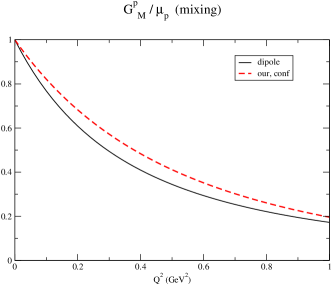
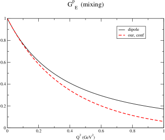
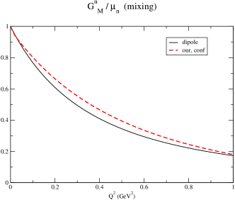
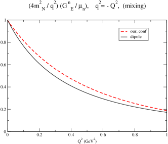
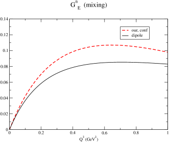
Figure 3: Sachs nucleon form factors in comparions with the dipole representation in the space–like region $Q\leq 1$ GeV².

In Table I we present the results for the magnetic moments and electromagnetic radii for this set of model parameters. In Fig. 3 we present our results for the $q^{2}$ dependence of electromagnetic form factors in the region $Q^{2}\in[0,1]\,{\rm GeV}^{2}$. Fig. 3 also shows plots of the dipole approximation to the form factors. The agreement of our results with the dipole approximation is satisfactory. Inclusion of chiral corrections as, for example, developed and discussed in Faessler:2005gd may lead to a further improvement in the low $Q^{2}$ description.

V $\Lambda$–type mass function and electromagnetic vertex

In a future publication we plan to study the rare baryon decays $\Lambda_{b}\to\Lambda_{s}\,\ell^{+}\ell^{-}$ in the context of the covariant quark model next . It is the purpose of this section to provide the necessary material that allows for a covariant quark model description of the $\Lambda=(Q[ud])$-type baryons composed of a $(s,c,b)$ quark Q and a light diquark-like state $[ud]$ with spin and isospin zero.

In general, for the $\Lambda$-type baryons one can construct three types of currents without derivatives — pseudoscalar $J^{P}$, scalar $J^{S}$ and axial-vector $J^{A}$ (see, Refs. Faessler:2001mr ; Branz:2010pq ; Ivanov:1996fj ; Ivanov:1999bu ):

$$J^{P}_{\Lambda_{Q[ud]}} = \epsilon^{a_{1}a_{2}a_{3}}\,Q^{a_{1}}\,u^{a_{2}}C\gamma_{5}d^{a_{3}}\,,$$

$$J^{S}_{\Lambda_{Q[ud]}} = \epsilon^{a_{1}a_{2}a_{3}}\,\gamma^{5}\,Q^{a_{1}}\,u^{a_{2}}Cd^{a_{3}}\,,$$

$$J^{A}_{\Lambda_{Q[ud]}} = \epsilon^{a_{1}a_{2}a_{3}}\,\gamma^{\mu}\,Q^{a_{1}}\,u^{a_{2}}C\gamma_{5}\gamma_{\mu}d^{a_{3}}\,.$$ (73)

There are only two independent linear combinations of the above three currents given by $J^{V}=(2J^{P}-2J^{S}+J^{A})/3$ and $J^{T}=J^{P}+J^{S}$. The symbol $[ud]$ denotes antisymmetrization of both flavor and spin indices w.r.t. the light quarks $u$ and $d$. We will consider three flavor types of the $\Lambda$-baryons: $\Lambda^{0}_{s}[ud]$, $\Lambda^{+}_{c}[ud]$ and $\Lambda^{0}_{b}[ud]$. In Ref. Faessler:2009xn we have shown that, in the nonrelativistic limit, the $J^{P}$ and $J^{A}$ interpolating currents of the $\Lambda_{Q[ud]}$ baryons become degenerate and attain the (same) correct nonrelativistic limit (in the case of single-heavy baryons this limit coincides with the heavy quark limit), while the $J^{S}$ current vanishes in the nonrelativistic limit. On the other hand, the $J^{P}$ and $J^{A}$ interpolating currents of $\Lambda$-type baryons become degenerate with their SU(N_f)-symmetric currents in the nonrelativistic limit. In Ref. Ivanov:1996fj we have shown that in case of the heavy-to-light baryon transition $\Lambda_{c}^{+}\to\Lambda^{0}e^{+}\nu_{e}$ the use of a SU(3) symmetric current for the $\Lambda^{0}$ hyperon is essential in order to describe data on $\Gamma(\Lambda_{c}^{+}\to\Lambda^{0}e^{+}\nu_{e})$ (see also discussion in Refs. Korner:1994nh ; Cheng:1995fe ). Therefore, in the following we restrict ourselves to the simplest pseudoscalar $J^{P}$ current. The nonlocal interpolating three–quark current is written as

$$J_{\Lambda}(x) = \int\!\!dx_{1}\!\!\int\!\!dx_{2}\!\!\int\!\!dx_{3}\,F_{\Lambda}(x;x_{1},x_{2},x_{3})\,J^{(\Lambda)}_{3q}(x_{1},x_{2},x_{3})\,,$$ (74)

$$J^{(\Lambda)}_{3q}(x_{1},x_{2},x_{3}) = \tfrac{1}{2}\epsilon^{a_{1}a_{2}a_{3}}\,Q_{a_{1}}(x_{1})\,\left(u^{a_{2}}(x_{2})\,C\,\gamma^{5}\,d^{a_{3}}(x_{3})-d^{a_{2}}(x_{3})\,C\,\gamma^{5}\,u^{a_{3}}(x_{2})\right)$$

$$= \epsilon^{a_{1}a_{2}a_{3}}\,Q^{a_{1}}(x_{1})\,u^{a_{2}}(x_{2})\,C\,\gamma^{5}\,d^{a_{3}}(x_{3})\,,$$

$$\bar{J}_{\Lambda}(x) = \int\!\!dx_{1}\!\!\int\!\!dx_{2}\!\!\int\!\!dx_{3}\,F_{\Lambda}(x;x_{1},x_{2},x_{3})\,\bar{J}^{(\Lambda)}_{3q}(x_{1},x_{2},x_{3})\,,$$

$$\bar{J}^{(\Lambda)}_{3q}(x_{1},x_{2},x_{3}) = \epsilon^{a_{1}a_{2}a_{3}}\,\bar{d}^{a_{3}}(x_{3})\,\gamma^{5}\,C\,\bar{u}^{a_{2}}(x_{2})\cdot\bar{Q}^{a_{1}}(x_{1})\,,$$

where $Q=s,c,b$.

The calculation of the $\Lambda$-type mass function and the electromagnetic vertex proceeds in the same way as in the nucleon case. The matrix elements in momentum space read

$$\Sigma_{\Lambda}(p)=6g_{\Lambda}^{2}\Big{\langle}\Big{\langle}\bar{\Phi}_{\Lambda}^{2}(-z_{0})S_{Q}(k_{1}+w_{1}p)\mbox{\rm{tr}}\left[S_{u}(k_{2}-w_{2}p)\gamma^{5}S_{d}(k_{2}-k_{1}+w_{3}p)\gamma^{5}\right]\Big{\rangle}\Big{\rangle}\,,$$ (75)

where we use the same short-hand notation $<<...>>$ for the two-fold loop-momentum integration as before (see Eqs. (44)). The variable $z_{0}$ is defined in (43).

The various contributions to the electromagnetic vertex are given by

$$\Lambda^{\mu}_{\Lambda\,Q}(p,p^{\prime}) = 6\,e_{Q}\,g_{\Lambda}^{2}\Big{\langle}\Big{\langle}\bar{\Phi}_{\Lambda}(-z_{0})\bar{\Phi}_{\Lambda}\Big{(}-\tfrac{1}{2}(k_{1}-k_{2}+w_{3}q)^{2}-\tfrac{1}{6}(k_{1}+k_{2}+(2w_{2}+w_{3})q)^{2}\Big{)}$$

$$\times S_{Q}(k_{1}+w_{1}p^{\prime})\gamma^{\mu}S_{Q}(k_{1}+w_{1}p^{\prime}+q)\mbox{\rm{tr}}\left[S_{u}(k_{2}-w_{2}p^{\prime})\gamma^{5}S_{d}(k_{2}-k_{1}+w_{3}p^{\prime})\gamma^{5}\right]\Big{\rangle}\Big{\rangle}\,,$$

$$\Lambda^{\mu}_{\Lambda\,u}(p,p^{\prime}) = -\,6\,e_{u}\,g_{\Lambda}^{2}\Big{\langle}\Big{\langle}\bar{\Phi}_{\Lambda}(-z_{0})\bar{\Phi}_{\Lambda}\Big{(}-\tfrac{1}{2}(k_{1}-k_{2}+w_{3}q)^{2}-\tfrac{1}{6}(k_{1}+k_{2}-(2w_{1}+w_{3})q)^{2}\Big{)}$$

$$\times S_{Q}(k_{1}+w_{1}p^{\prime})\mbox{\rm{tr}}\left[S_{u}(k_{2}-w_{2}p^{\prime}-q)\gamma^{\mu}S_{u}(k_{2}-w_{2}p^{\prime})\gamma^{5}S_{d}(k_{2}-k_{1}+w_{3}p^{\prime})\gamma^{5}\right]\Big{\rangle}\Big{\rangle}\,,$$

$$\Lambda^{\mu}_{\Lambda\,d}(p,p^{\prime}) = 6\,e_{d}\,g_{\Lambda}^{2}\Big{\langle}\Big{\langle}\bar{\Phi}_{\Lambda}(-z_{0})\bar{\Phi}_{\Lambda}\Big{(}-\tfrac{1}{2}(k_{1}-k_{2}-(w_{1}+w_{2})q)^{2}-\tfrac{1}{6}(k_{1}+k_{2}-(w_{1}-w_{2})q)^{2}\Big{)}$$

$$\times S_{Q}(k_{1}+w_{1}p^{\prime})\mbox{\rm{tr}}\left[S_{u}(k_{2}-w_{2}p^{\prime})\gamma^{5}S_{d}(k_{2}-k_{1}+w_{3}p^{\prime})\gamma^{\mu}S_{d}(k_{2}-k_{1}+w_{3}p^{\prime}+q)\gamma^{5}\right]\Big{\rangle}\Big{\rangle}\,,$$

$$\Lambda^{\mu}_{\Lambda\,(a)}(p,p^{\prime}) = 6\,g_{\Lambda}^{2}\Big{\langle}\Big{\langle}\bar{\Phi}_{\Lambda}(-z_{0})\tilde{E}_{\Lambda}^{\mu}(k_{1}+w_{1}p^{\prime},-k_{2}+w_{2}p^{\prime},k_{2}-k_{1}+w_{3}p^{\prime};q)$$

$$\times S_{Q}(k_{1}+w_{1}p^{\prime})\mbox{\rm{tr}}\left[S_{u}(k_{2}-w_{2}p^{\prime})\gamma^{5}S_{d}(k_{2}-k_{1}+w_{3}p^{\prime})\gamma^{5}\right]\Big{\rangle}\Big{\rangle}\,,$$

$$\Lambda^{\mu}_{\Lambda\,(b)}(p,p^{\prime}) = 6\,g_{\Lambda}^{2}\langle\langle\bar{\Phi}_{\Lambda}(-z_{0})\tilde{E}_{\Lambda}^{\mu}(k_{1}+w_{1}p,-k_{2}+w_{2}p,k_{2}-k_{1}+w_{3}p;-q)$$ (76)

$$\times S_{Q}(k_{1}+w_{1}p)\mbox{\rm{tr}}\left[S_{u}(k_{2}-w_{2}p)\gamma^{5}S_{d}(k_{2}-k_{1}+w_{3}p)\gamma^{5}\right]\Big{\rangle}\Big{\rangle}\,.$$

One now has three e.m. vertex contributions because there are three different quarks in the $\Lambda_{Q}$ state. The function $\tilde{E}_{\Lambda}^{\mu}(r_{1},r_{2}.r_{3};r)$ has been defined in Eq. (28). The variables $q_{1}=\sum_{i=1}^{3}w_{i1}r_{i}$ and $q_{2}=\sum_{i=1}^{3}w_{i2}r_{i}$ in $\tilde{E}_{\Lambda}^{\mu}(r_{1},r_{2}.r_{3};r)$ can be seen to be related to the loop momenta by

$$q_{1}=\tfrac{1}{\sqrt{2}}(k_{1}-k_{2})\,,\qquad q_{2}=-\,\tfrac{1}{\sqrt{6}}(k_{1}+k_{2})$$ (77)

for both bubble diagrams. By using Eq. (77) one finds the $q=0$ relations

$$\Lambda^{\mu}_{\Lambda\,(a)}(p,p)+\Lambda^{\mu}_{\Lambda\,(b)}(p,p) = -\,8\,g_{\Lambda}^{2}\Big{\langle}\Big{\langle}(Q_{1}k_{1}^{\mu}+Q_{2}k_{2}^{\mu})\bar{\Phi}^{\prime}_{\Lambda}(-z_{0})\bar{\Phi}_{\Lambda}(-z_{0})$$

$$\times S_{Q}(k_{1}+w_{1}p)\mbox{\rm{tr}}\left[S_{u}(k_{2}-w_{2}p)\gamma^{5}S_{d}(k_{2}-k_{1}+w_{3}p)\gamma^{5}\right]\Big{\rangle}\Big{\rangle}\,,$$

$$Q_{1} = e_{1}(w_{2}+2w_{3})-e_{2}(w_{1}-w_{3})-e_{3}(2w_{1}+w_{2})\,,$$

$$Q_{2} = e_{1}(w_{2}-w_{3})-e_{2}(w_{1}+2w_{3})+e_{3}(w_{1}+2w_{2})\,.$$ (78)

where the subscripts on the charges $e_{i}$ refer to the flavors of the three quarks: $"i=1"\to"s,c,b"$, $"i=2"\to"u"$ and $"i=3"\to"d"$. Next we will use an IBP-identity to write

$$\Big{\langle}\Big{\langle}\frac{\partial}{\partial k_{i}^{\mu}}\Big{\{}\bar{\Phi}^{2}_{\Lambda}(-z_{0})S_{Q}(k_{1}+w_{1}p)\mbox{\rm{tr}}\left[S_{u}(k_{2}-w_{2}p)\gamma^{5}S_{d}(k_{2}-k_{1}+w_{3}p)\gamma^{5}\right]\Big{\}}\Big{\rangle}\Big{\rangle}\,\equiv\,0\,,\qquad(i=1,2)\,.$$ (79)

One finds

$$\Big{\langle}\Big{\langle}k_{1}^{\mu}\,A_{0}\Big{\rangle}\Big{\rangle} = \frac{1}{4}\Big{\langle}\Big{\langle}(2\,A^{\mu}_{1}+A^{\mu}_{2}-A^{\mu}_{3})\Big{\rangle}\Big{\rangle}\,,$$

$$\Big{\langle}\Big{\langle}k_{2}^{\mu}\,A_{0}\Big{\rangle}\Big{\rangle} = \frac{1}{4}\Big{\langle}\Big{\langle}(A^{\mu}_{1}+2\,A^{\mu}_{2}+A^{\mu}_{3})\Big{\rangle}\Big{\rangle}\,,$$ (80)

where

$$A_{0} = \bar{\Phi}^{\prime}_{\Lambda}(-z_{0})\,\bar{\Phi}_{\Lambda}(-z_{0})S_{Q}(k_{1}+w_{1}p)\mbox{\rm{tr}}\left[S_{u}(k_{2}-w_{2}p)\gamma^{5}S_{d}(k_{2}-k_{1}+w_{3}p)\gamma^{5}\right]\,,$$

$$A^{\mu}_{1} = \bar{\Phi}^{2}_{\Lambda}(-z_{0})S_{Q}(k_{1}+w_{1}p)\gamma^{\mu}S_{Q}(k_{1}+w_{1}p)\mbox{\rm{tr}}\left[S_{u}(k_{2}-w_{2}p)\gamma^{5}S_{d}(k_{2}-k_{1}+w_{3}p)\gamma^{5}\right]\,,$$

$$A^{\mu}_{2} = \bar{\Phi}^{2}_{\Lambda}(-z_{0})S_{Q}(k_{1}+w_{1}p)\mbox{\rm{tr}}\left[S_{u}(k_{2}-w_{2}p)\gamma^{\mu}S_{u}(k_{2}-w_{2}p)\gamma^{5}S_{d}(k_{2}-k_{1}+w_{3}p)\gamma^{5}\right]\,,$$

$$A^{\mu}_{3} = \bar{\Phi}^{2}_{\Lambda}(-z_{0})S_{Q}(k_{1}+w_{1}p)\mbox{\rm{tr}}\left[S_{u}(k_{2}-w_{2}p)\gamma^{5}S_{d}(k_{2}-k_{1}+w_{3}p)\gamma^{\mu}S_{d}(k_{2}-k_{1}+w_{3}p)\gamma^{5}\right]\,.$$ (81)

Using these identities and collecting all pieces together, one has

$$\Lambda^{\mu}_{\Lambda}(p,p)=(e_{Q}+e_{u}+e_{d})\,\frac{\partial\Sigma_{\Lambda}(p)}{\partial p^{\mu}}\,,\qquad\not\!p=m_{\Lambda}\,.$$ (82)

As was discussed above, this Ward identity allows one to use the compositeness condition $Z_{\Lambda}=0$ written in the form

$$\Lambda^{\mu}_{\Lambda}(p,p)=\gamma^{\mu}\,,\qquad\not\!p=m_{\Lambda}\,,$$ (83)

where we take $e_{Q}=e_{c}$ for the present discussion. Again we have checked analytically that, on the $\Lambda$-type baryon mass shell, the vertex diagrams are gauge invariant by themselves and the non-gauge invariant parts coming from the bubble diagrams corresponding to Fig.2(c) and 2(d) cancel each other before $t$-integration. The standard definition of the electromagnetic form factors is

$$\Lambda^{\mu}_{\Lambda}(p,p^{\prime})=\gamma_{\mu}F_{1}(q^{2})-\frac{i\sigma^{\mu q}}{2m_{\Lambda}}F_{2}(q^{2})\,,$$ (84)

where $\sigma^{\mu q}=\tfrac{i}{2}(\gamma^{\mu}\gamma^{\nu}-\gamma^{\nu}\gamma^{\mu})q_{\nu}.$ The magnetic moment of the $\Lambda$-type baryon is defined by

$$\mu_{\Lambda}\,=\,\left(\,F_{1}(0)+F_{2}(0)\,\right)\,\,\frac{e}{2m_{\Lambda}}\,.$$ (85)

In terms of the nuclear magneton (n.m.) $\frac{e}{2m_{p}}$ the $\Lambda$-type baryon magnetic moment the $\Lambda$–hyperon magnetic moment is given by

$$\mu_{\Lambda}=\ (\,F_{1}(0)+F_{2}(0)\,)\,\,\frac{m_{p}}{m_{\Lambda}}\,,$$ (86)

where $m_{p}$ is the proton mass.

In the present paper we shall only make a rather cursory investigation into the possible values of the size parameters of the $\Lambda=(Q[ud])$-type baryons. A more detailed investigation will be left to our future publication next where we will include information on the charged current transitions $\Lambda_{b}\to\Lambda_{c}$ and $\Lambda_{c}\to\Lambda_{s}$ to specify the values of the size parameters of the $\Lambda=(Q[ud])$-type baryons.

Let us assume for the moment that the size parameters are the same for all $\Lambda$-type baryons. One then has

$$\Lambda_{\Lambda} = 0.5\,{\rm GeV}\quad\mu_{\Lambda_{s}}=-0.73\,,\quad\mu_{\Lambda_{c}}=+0.36\,,\quad\mu_{\Lambda_{b}}=-0.06\,,$$

$$\Lambda_{\Lambda} = 1.0\,{\rm GeV}\quad\mu_{\Lambda_{s}}=-0.68\,,\quad\mu_{\Lambda_{c}}=+0.40\,,\quad\mu_{\Lambda_{b}}=-0.06\,,$$

$$\Lambda_{\Lambda} = 1.5\,{\rm GeV}\quad\mu_{\Lambda_{s}}=-0.61\,,\quad\mu_{\Lambda_{c}}=+0.44\,,\quad\mu_{\Lambda_{b}}=-0.07\,.$$ (87)

The magnetic moment of the $\Lambda_{s}$ has to be compared with the experimental value listed in Nakamura:2010zzi

$$\mu_{\Lambda_{s}}=-\,0.613\pm 0.004\,.$$ (88)

Eq. (87) shows that the value of the magnetic moment of the $\Lambda_{s}$ is quite stable against variations of its size parameter. There is no experimental information on the magnetic moments of the $\Lambda_{b}$ and $\Lambda_{c}$.

The calculation of the form factors in our approach is automated by the use of FORM and FORTRAN packages written for this purpose. In order to be able to compare with our earlier unconfined calculations we have written two versions for the confined and the unconfined versions of the covariant quark model.

VI Summary and conclusions

We have extended our previous formulation of the confined covariant quark model for mesons and tetraquark states to the baryon sector. We have discussed in some detail various calculational aspects of the two-loop baryon problem such as the evaluation of the baryon mass operator and its derivative, the implementation of confinement in the two–loop context, the calculation of electromagnetic current-induced transition matrix elements and the analytical verification of the pertinent Ward and Ward–Takahashi identities associated with the electromagnetic matrix elements.

In our numerical work we have used the same values of the constituent quark masses and infrared cutoff as had been obtained before in the meson sector by a fit to various mesonic transition matrix elements. In this way the number of model parameters were kept to a minimum.

Using two parameters we have calculated the nucleon magnetic moments and charge radii as well as the electromagnetic form factors at low momentum transfers. An extension of our work to the $N-\Delta(1236)$ transition can be done along the lines described in Faessler:2006ky .

We have also discussed light and heavy $\Lambda=(Q[ud])$-type baryons. In particular we obtained a value for the size parameter of the $\Lambda_{s}$ by a fit to its experimentally known magnetic moment. By determining the properties of the $\Lambda=(Q[ud])$-type baryons we have laid the groundwork for a calculation of the rare decays of the $\Lambda_{b}$-baryon (such as $\Lambda_{b}\to\Lambda_{s}\ell^{+}\ell^{-}$) within the framework of the covariant quark model.

Table 1: Electromagnetic properties of nucleons 

Quantity	Our results	Data Nakamura:2010zzi
$\mu_{p}$ (in n.m.)	2.96	2.793
$\mu_{n}$ (in n.m.)	-1.83	-1.913
$r_{E}^{p}$ (fm)	0.805	0.8768 $\pm$ 0.0069
$\langle r^{2}_{E}\rangle^{n}$ (fm2)	-0.121	-0.1161 $\pm$ 0.0022
$r_{M}^{p}$ (fm)	0.688	0.777 $\pm$ 0.013 $\pm$ 0.010
$r_{M}^{n}$ (fm)	0.685	0.862${}^{+0.009}_{-0.008}$

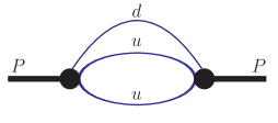
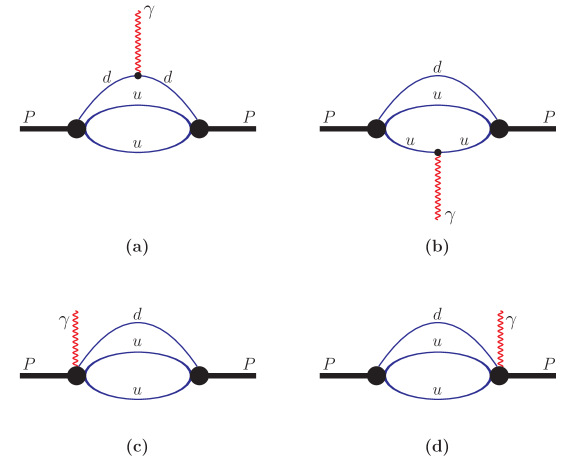
Figure 1: Proton mass operator.

Figure 2: Electromagnetic vertex function of the proton: (a) vertex diagram with the e.m. current attached to d-quark; (b) vertex diagram with the e.m. current attached to u-quark; (c) bubble diagram with the e.m. current attached to the initial state vertex; (d) the bubble diagram with e.m. current attached to the final state vertex.

References

• (1) A. Faessler, T. Gutsche, M. A. Ivanov, J. G. Körner and V. E. Lyubovitskij, Phys. Lett. B 518 (2001) 55 [hep-ph/0107205].
• (2) A. Faessler, T. Gutsche, B. R. Holstein, M. A. Ivanov, J. G. Körner and V. E. Lyubovitskij, Phys. Rev. D 78 (2008) 094005 [arXiv:0809.4159 [hep-ph]].
• (3) A. Faessler, T. Gutsche, M. A. Ivanov, J. G. Körner and V. E. Lyubovitskij, Phys. Rev. D 80 (2009) 034025 [arXiv:0907.0563 [hep-ph]].
• (4) T. Branz, A. Faessler, T. Gutsche, M. A. Ivanov, J. G. Körner, V. E. Lyubovitskij and B. Oexl, Phys. Rev. D 81 (2010) 114036 [arXiv:1005.1850 [hep-ph]].
• (5) T. Branz, A. Faessler, T. Gutsche, M. A. Ivanov, J. G. Körner and V. E. Lyubovitskij, Phys. Rev. D 81 (2010) 034010 [arXiv:0912.3710 [hep-ph]].
• (6) M. A. Ivanov, J. G. Körner, S. G. Kovalenko, P. Santorelli and G. G. Saidullaeva, Phys. Rev. D 85, 034004 (2012) [arXiv:1112.3536 [hep-ph]].
• (7) S. Dubnicka, A. Z. Dubnickova, M. A. Ivanov, J. G. Körner, Phys. Rev.  D81, 114007 (2010). [arXiv:1004.1291 [hep-ph]]; S. Dubnicka, A. Z. Dubnickova, M. A. Ivanov, J. G. Körner and G. G. Saidullaeva, AIP Conf. Proc.  1343, 385 (2011) [arXiv:1011.4417 [hep-ph]].
• (8) S. Dubnicka, A. Z. Dubnickova, M. A. Ivanov, J. G. Körner, P. Santorelli and G. G. Saidullaeva, Phys. Rev. D 84, 014006 (2011) [arXiv:1104.3974 [hep-ph]].
• (9) T. Gutsche, M. A. Ivanov, J. G. Körner, V. E. Lyubovitskij and P. Santorelli, in preparation.
• (10) W. R. B. de Araujo, T. Frederico, M. Beyer and H. J. Weber, Int. J. Mod. Phys. A 18, 5767 (2003) [hep-ph/0305120].
• (11) M. A. Ivanov, M. P. Locher and V. E. Lyubovitskij, Few Body Syst.  21 (1996) 131.
• (12) S. Weinberg, Phys. Rev.  130, 776 (1963).
• (13) A. Salam, Nuovo Cim.  25, 224 (1962).
• (14) K. Hayashi, M. Hirayama, T. Muta, N. Seto and T. Shirafuji, Fortsch. Phys. 15, 625 (1967).
• (15) G. V. Efimov and M. A. Ivanov, The Quark Confinement Model of Hadrons, (IOP Publishing, Bristol $\&$ Philadelphia, 1993).
• (16) J. A. M. Vermaseren, Nucl. Phys. Proc. Suppl.  183, 19 (2008) [arXiv:0806.4080 [hep-ph]]; arXiv:math-ph/0010025. S. Dubnicka, A. Z. Dubnickova, M. A. Ivanov and J. G. Körner, Phys. Rev. D 81, 114007 (2010) [arXiv:1004.1291 [hep-ph]].
• (17) S. Mandelstam, Annals Phys.  19, 1 (1962).
• (18) J. Terning, Phys. Rev. D 44, 887 (1991).
• (19) A. Faessler, T. Gutsche, M. A. Ivanov, J. G. Körner, V. E. Lyubovitskij, D. Nicmorus and K. Pumsa-ard, Phys. Rev. D 73, 094013 (2006) [hep-ph/0602193].
• (20) K. Nakamura et al. [ Particle Data Group Collaboration ], J. Phys. G G37 (2010) 075021.
• (21) A. Faessler, T. .Gutsche, V. E. Lyubovitskij and K. Pumsa-ard, Phys. Rev. D 73 (2006) 114021 [hep-ph/0511319].
• (22) M. A. Ivanov, V. E. Lyubovitskij, J. G. Körner and P. Kroll, Phys. Rev. D 56, 348 (1997) [arXiv:hep-ph/9612463].
• (23) M. A. Ivanov, J. G. Körner, V. E. Lyubovitskij and A. G. Rusetsky, Phys. Lett. B 476, 58 (2000) [arXiv:hep-ph/9910342].
• (24) J. G. Körner, M. Krämer and D. Pirjol, Prog. Part. Nucl. Phys.  33, 787 (1994) [hep-ph/9406359].
• (25) H. -Y. Cheng and B. Tseng, Phys. Rev. D 53 (1996) 1457 [Erratum-ibid. D 55 (1997) 1697] [hep-ph/9502391].
• (26) A. Faessler, T. Gutsche, B. R. Holstein, V. E. Lyubovitskij, D. Nicmorus and K. Pumsa-ard, Phys. Rev. D 74, 074010 (2006) [hep-ph/0608015].