Parity violation in radiative neutron capture on deuteron

Abstract

Parity violating (PV) effects in neutron-deuteron radiative capture are studied using Desplanques, Donoghue, and Holstein (DDH) and effective field theory weak potentials. The values of PV effects are calculated using wave functions, obtained by solving three-body Faddeev equations in configuration space for phenomenological strong potentials. The relations between physical observables and low-energy constants are presented, and dependencies of the calculated PV effects on strong and weak potentials are discussed. The presented analysis shows the possible reason for the existing discrepancy in PV nuclear data analysis using the DDH approach and reveals a new opportunity to study short range interactions in nuclei.

I Introduction

Low energy parity violating (PV) effects play an important role in understanding the main features of the Standard model. Many nuclear PV effects were measured and calculated during the last several years. Despite the fact that existing calculations of nuclear PV effects are in a reasonably good agreement with the measured ones, lately it became clear (see, for example Zhu et al. (2005); Holstein (2005a); Desplanque (2005); Ramsey-Musolf and Page (2006) and references therein) that it is rather difficult to describe the available experimental data with the same set of weak nucleon coupling constants using the traditional DDH Desplanques et al. (1980a) weak meson exchange potential.

As a possible solution for this problem, a new approach, based on the effective field theory (EFT), has been introduced to parameterize the PV effects in a model independent way (see, papers Zhu et al. (2005); Ramsey-Musolf and Page (2006); Liu (2007) and references therein). The main goal of the EFT approach is to describe a large number of PV effects in terms of a small number of constants (LEC), which are the free parameters of the theory. Unfortunately, since the number of experimentally measured (and independent in terms of unknown LECs) PV effects in two body systems is not enough to constrain all LECs Girlanda (2008); Phillips et al. (2009); Shin et al. (2010); Schindler and Springer (2009). In order to determine these constants it is necessary to include also the data obtained on heavier nuclear systems.

Furthermore one should better understand PV effects in heavier nuclei because these effects might be essentially enhanced Sushkov and Flambaum (1982); Bunakov and Gudkov (1983); Gudkov (1992) in many body systems. However, how to apply the EFT approach for the calculations of PV effects in nuclei it is still an open question.

To verify the possible issues related to the application of the DDH description of PV effects in nuclei and the possibility of systematic calculations of PV effects in nuclei using EFT approach, it is desirable to start from the calculations of PV effects in the simplest nuclear systems, such as neutron-deuteron (n-d) compound. PV effects for the elastic n-d scattering have been calculated recently Schiavilla et al. (2008); Song et al. (2011a) using both DDH and EFT approaches. However, before extending these techniques to the many-body nuclear systems, it is important to consider inelastic processes which are usually more sensitive to short range interactions.

With this aim, we present in this paper a comprehensive analysis of PV effects in neutron-deuteron radiative capture Moskalev (1969); E. Hadjimichael and Newton (1974); McKellar (1974); Desplanques and Benayoun (1986) using weak potential of DDH-type, as well as weak potentials obtained in pionless and pionful EFT. For the strong interaction, we have tested several realistic nucleon-nucleon potentials, also in conjunction with three-nucleon force. Three-nucleon wave functions have been obtained by solving Faddeev equations in configuration space for the complete Hamiltonians comprising both weak and strong interactions.

The paper is structured as follows. In the next section, a brief description of the employed formalism is presented. Then, we discuss the results of our calculations and perform a detailed analysis of model and cutoff dependence of the calculated PV parameters. In conclusion, the implications of our result are summarized.

II Formalism

We consider three parity violating observables in the radiative neutron capture on deuterons ($n+d\to^{3}H+\gamma$): circular polarization of the emitted photons ($P^{\gamma}$), asymmetry of the photons in relation to neutron polarization ($a_{n}^{\gamma}$), and asymmetry of the photons in relation to deuteron polarization ($A_{d}^{\gamma}$). For low energy neutrons, the expressions for these PV effects could be written in terms of parity conserving magnetic dipole ($M1$) and parity violating electric dipole ($E1$) transition matrix elements as:

$$a^{\gamma}_{n}(E) = \frac{2}{3}\frac{{\rm Re}\left[\sqrt{2}(E1^{*}_{\frac{3}{2}}M1_{\frac{1}{2}}+E1^{*}_{\frac{1}{2}}M1_{\frac{3}{2}})+\frac{5}{2}(E1^{*}_{\frac{3}{2}}M1_{\frac{3}{2}})-(E1^{*,(+)}_{\frac{1}{2}}M1_{\frac{1}{2}})\right]}{|M1_{\frac{1}{2}}|^{2}+|M1_{\frac{3}{2}}|^{2}},$$

$$P^{\gamma}(E) = \frac{2{\rm Re}\left[E1^{*}_{\frac{1}{2}}M1_{\frac{1}{2}}+E1^{*}_{\frac{3}{2}}M1_{\frac{3}{2}}\right]}{|M1_{\frac{1}{2}}|^{2}+|M1_{\frac{3}{2}}|^{2}},$$

$$A^{\gamma}_{d}(E) = -\frac{{\rm Re}\left[-5E1^{*}_{\frac{3}{2}}M1_{\frac{3}{2}}-4E1^{*}_{\frac{1}{2}}M1_{\frac{1}{2}}+\sqrt{2}E1^{*}_{\frac{3}{2}}M1_{\frac{1}{2}}+\sqrt{2}E1^{*}_{\frac{1}{2}}M1_{\frac{3}{2}}\right]}{2(|M1_{\frac{1}{2}}|^{2}+|M1_{\frac{3}{2}}|^{2})}.$$ (1)

Here the M1 and E1 amplitudes are defined as reduced matrix elements of the multipole operators

$$X1_{J}\equiv\langle-{\boldsymbol{q}},J_{B}||\hat{T}_{1}^{X}||J\rangle,\quad\mbox{ with }X=(M,E),$$ (2)

where $J_{B}$ and $J$ are total angular momenta of bound state and scattering state respectively, and ${\boldsymbol{q}}$ is a momentum of the outgoing photon. The electromagnetic multipole operators in the limit of small $q$ can be written as

$${\hat{T}}^{Mag}_{JM}(q) \simeq -\frac{q^{J}}{i(2J+1)!!}\sqrt{\frac{J+1}{J}}\int d{\bf x}[\hat{\bf\mu}({\bf x})+\frac{1}{J+1}{\bf r}\times\hat{\bf J}_{c}(x)]\cdot\nabla(x^{J}Y_{JM})$$

$${\hat{T}}^{El}_{JM}(q) \simeq \frac{q^{J}}{(2J+1)!!}\sqrt{\frac{J+1}{J}}\int d{\bf x}(x^{J}Y_{JM}\hat{\rho}(x)-\frac{iq}{J+1}\hat{\bf\mu}(x)\cdot[{\boldsymbol{r}}\times\nabla x^{J}Y_{JM}]),$$

where $\hat{J}_{c}(x)$ is a convection current, $\hat{\mu}(x)$ is a magnetization current, $\hat{\rho}(x)$ is a charge operator, and $q=\omega$ is the energy of photon. In our calculations, we use $M1$ operator up to $N^{3}LO$ in chiral order counting, which includes contributions from two-pion exchange and contact currents obtained in heavy baryon chiral perturbation theorySong et al. (2009). For calculations of E1 amplitudes at the leading order, we use only E1 charge operator, which is related to 3-vector currents by Siegert’s theorem. Since, in the used spherical harmonics convention both parity conserving $M1$ and parity violating $E1$ amplitudes are purely imaginary, it is convenient to define real-valued $\widetilde{\cal M}_{J}$ and $\widetilde{\cal E}_{J}$ matrix elements as

$$M1_{J} = i\frac{\omega\mu_{N}}{\sqrt{6\pi}\sqrt{4\pi}}\widetilde{\cal M}_{J},\quad E1_{J}=-i\frac{\omega}{\sqrt{6\pi}}\widetilde{\cal E}_{J},$$ (3)

where $\mu_{N}=\frac{1}{2m_{N}}$.

The calculations of parity conserving $M1$ amplitudes for radiative n-d capture have been reported in papers Song et al. (2009); Pastore et al. (2009) using the hybrid method, where the wave functions were obtained from phenomenological potential models and the current operators were derived from the heavy baryon chiral effective field theory. The results of these calculations can be approximated Song et al. (2009) by the following expressions

$$\widetilde{\cal M}_{\frac{1}{2}} = +21.87+10.76[(B_{model}/B_{exp})^{-2.5}-1]\mbox{ fm}^{\frac{3}{2}},$$

$$\widetilde{\cal M}_{\frac{3}{2}} = -12.24-11.35[(B_{model}/B_{exp})^{-2.5}-1]\mbox{ fm}^{\frac{3}{2}},$$ (4)

where two low energy constants of two-body M1 operators are fixed Song et al. (2009) by experimental values of ${}^{3}H$ and ${}^{3}He$ magnetic moments. In these expressions, M1 amplitudes and the binding energy of ${}^{3}H$, $B_{model}$ depends on the strong interaction model. However, the observed explicit correlation between the calculated The M1 amplitudes and the binding energy $B_{model}$ provides the unique opportunity to eliminate the model dependence. This might be done by setting in eq.(4) $B_{model}/B_{exp}=1$. M1 amplitudes obtained in such a way lead to the value of the total neutron-deutron radiative capture cross section $\sigma_{tot}=0.49(1)$ mb, which is well consistent with the experimental data.

E1 amplitudes are calculated using three-body wave functions, which are obtained by solving Faddeev equations in configuration space. We have tested different combinations of strong and weak potentials. For the strong (parity conserving) part of the Hamiltonian, we choose one of the realistic nucleon-nucleon interaction models, namely: AV18, Reid, NijmII and INOY were employed. Also we have performed calculations for AV18 NN potential in conjunction with UIX three-nucleon force (denoted as AV18+UIX). For the parity violating part of the Hamiltonian - one of the weak potentials was employed, which was treated as perturbation. In this paper, we consider three types of parity violating weak potentials: the standard DDH potential with meson exchange nucleon-nucleon interactions, the potential derived from pionless version, and the potential derived from pionful version of effective field theory. Our approach could be considered as a hybrid method, which is similar to the hybrid approach in the line of Weinberg’s scheme and which has been successfully applied for the calculations of weak and electromagnetic processes involving three-body and four-body hadronic systems Song et al. (2007, 2009); Lazauskas et al. (2009); Park et al. (2003); Pastore et al. (2009); Girlanda et al. (2010), as well as for calculations of parity violating Song et al. (2011a) and time reversal violating effects in elastic n-d scattering Song et al. (2011b, c). It is worth mentioning that alternative calculations of parity violating effects in elastic n-d scattering using pionless EFT Griesshammer et al. (2012) are well consistent with the hybrid calculations Song et al. (2011a), though the detailed comparison between these two methods is required.

II.1 The parity violating potentials

To understand the possible difference in the description of parity violating effects by DDH and EFT-type of potentials, we compare the operator structure of the potentials for the DDH potential Desplanques et al. (1980b) and for two different choices of EFT potentials Zhu et al. (2005) which are derived from pionless and pionful EFT Lagrangian. All these potentials can be expanded in terms of $O^{(n)}_{ij}$ operators Schiavilla et al. (2008) as

$$v_{ij}^{\alpha}=\sum_{n}c_{n}^{\alpha}O^{(n)}_{ij},\quad\mbox{$\alpha=$ DDH, pionless EFT or pionful EFT}$$ (5)

with the explicit forms for the operators $O^{(n)}_{ij}$ and corresponding parameters $c_{n}^{\alpha}$ listed in table 1 , where coefficients $c_{n}^{\alpha}$ have dimension of $[\mbox{fm}]$ and scalar functions $f_{n}^{\alpha}(r)$ have dimension of $[\mbox{fm}^{-1}]$.

Table 1: Parameters and operators of parity violating potentials. $g_{A}=1.26$, $F_{\pi}=92.4$ MeV. ${\cal T}_{ij}\equiv(3\tau_{i}^{z}\tau_{j}^{z}-\tau_{i}\cdot\tau_{j})$. Scalar function $\tilde{L}_{\Lambda}(r)\equiv 3L_{\Lambda}(r)-H_{\Lambda}(r)$.

$n$	$c_{n}^{DDH}$	$f_{n}^{DDH}(r)$	$c_{n}^{\not{\pi}}$	$f_{n}^{\not{\pi}}(r)$	$c_{n}^{\pi}$	$f_{n}^{\pi}(r)$	$O^{(n)}_{ij}$
$1$	$+\frac{g_{\pi}}{2\sqrt{2}m_{N}}h_{\pi}^{1}$	$f_{\pi}(r)$	$-\frac{\mu^{2}C_{6}^{\not{\pi}}}{\Lambda_{\chi}^{3}}$	$f^{\not{\pi}}_{\mu}(r)$	$+\frac{g_{\pi}}{2\sqrt{2}m_{N}}h_{\pi}^{1}$	$f^{\pi}_{\Lambda}(r)$	$(\tau_{i}\times\tau_{j})^{z}({\boldsymbol{\sigma}}_{i}+{\boldsymbol{\sigma}}_{j})\cdot{\boldsymbol{X}}^{(1)}_{ij,-}$
$2$	$-\frac{g_{\rho}}{m_{N}}h_{\rho}^{0}$	$f_{\rho}(r)$	$0$	$0$	$0$	$0$	$(\tau_{i}\cdot\tau_{j})({\boldsymbol{\sigma}}_{i}-{\boldsymbol{\sigma}}_{j})\cdot{\boldsymbol{X}}^{(2)}_{ij,+}$
$3$	$-\frac{g_{\rho}(1+\kappa_{\rho})}{m_{N}}h_{\rho}^{0}$	$f_{\rho}(r)$	$0$	$0$	$0$	$0$	$(\tau_{i}\cdot\tau_{j})({\boldsymbol{\sigma}}_{i}\times{\boldsymbol{\sigma}}_{j})\cdot{\boldsymbol{X}}^{(3)}_{ij,-}$
$4$	$-\frac{g_{\rho}}{2m_{N}}h_{\rho}^{1}$	$f_{\rho}(r)$	$\frac{\mu^{2}}{\Lambda^{3}_{\chi}}(C^{\not{\pi}}_{2}+C^{\not{\pi}}_{4})$	$f_{\mu}^{\not{\pi}}(r)$	$\frac{\Lambda^{2}}{\Lambda^{3}_{\chi}}(C^{\pi}_{2}+C^{{\pi}}_{4})$	$f_{\Lambda}(r)$	$(\tau_{i}+\tau_{j})^{z}({\boldsymbol{\sigma}}_{i}-{\boldsymbol{\sigma}}_{j})\cdot{\boldsymbol{X}}^{(4)}_{ij,+}$
$5$	$-\frac{g_{\rho}(1+\kappa_{\rho})}{2m_{N}}h_{\rho}^{1}$	$f_{\rho}(r)$	$0$	$0$	$\frac{2\sqrt{2}\pi g_{A}^{3}\Lambda^{2}}{\Lambda_{\chi}^{3}}h^{1}_{\pi}$	$L^{\pi}_{\Lambda}(r)$	$(\tau_{i}+\tau_{j})^{z}({\boldsymbol{\sigma}}_{i}\times{\boldsymbol{\sigma}}_{j})\cdot{\boldsymbol{X}}^{(5)}_{ij,-}$
$6$	$-\frac{g_{\rho}}{2\sqrt{6}m_{N}}h_{\rho}^{2}$	$f_{\rho}(r)$	$-\frac{2\mu^{2}}{\Lambda^{3}_{\chi}}C_{5}^{\not{\pi}}$	$f^{\not{\pi}}_{\mu}(r)$	$-\frac{2\Lambda^{2}}{\Lambda^{3}_{\chi}}C_{5}^{{\pi}}$	$f_{\Lambda}(r)$	${\cal T}_{ij}({\boldsymbol{\sigma}}_{i}-{\boldsymbol{\sigma}}_{j})\cdot{\boldsymbol{X}}^{(6)}_{ij,+}$
$7$	$-\frac{g_{\rho}(1+\kappa_{\rho})}{2\sqrt{6}m_{N}}h_{\rho}^{2}$	$f_{\rho}(r)$	$0$	$0$	$0$	$0$	${\cal T}_{ij}({\boldsymbol{\sigma}}_{i}\times{\boldsymbol{\sigma}}_{j})\cdot{\boldsymbol{X}}^{(7)}_{ij,-}$
$8$	$-\frac{g_{\omega}}{m_{N}}h_{\omega}^{0}$	$f_{\omega}(r)$	$\frac{2\mu^{2}}{\Lambda^{3}_{\chi}}C_{1}^{\not{\pi}}$	$f_{\mu}^{\not{\pi}}(r)$	$\frac{2\Lambda^{2}}{\Lambda^{3}_{\chi}}C_{1}^{{\pi}}$	$f_{\Lambda}(r)$	$({\boldsymbol{\sigma}}_{i}-{\boldsymbol{\sigma}}_{j})\cdot{\boldsymbol{X}}^{(8)}_{ij,+}$
$9$	$-\frac{g_{\omega}(1+\kappa_{\omega})}{m_{N}}h_{\omega}^{0}$	$f_{\omega}(r)$	$\frac{2\mu^{2}}{\Lambda_{\chi}^{3}}\tilde{C}^{\not{\pi}}_{1}$	$f_{\mu}^{\not{\pi}}(r)$	$\frac{2\Lambda^{2}}{\Lambda_{\chi}^{3}}\tilde{C}^{{\pi}}_{1}$	$f_{\Lambda}(r)$	$({\boldsymbol{\sigma}}_{i}\times{\boldsymbol{\sigma}}_{j})\cdot{\boldsymbol{X}}^{(9)}_{ij,-}$
$10$	$-\frac{g_{\omega}}{2m_{N}}h_{\omega}^{1}$	$f_{\omega}(r)$	$0$	$0$	$0$	$0$	$(\tau_{i}+\tau_{j})^{z}({\boldsymbol{\sigma}}_{i}-{\boldsymbol{\sigma}}_{j})\cdot{\boldsymbol{X}}^{(10)}_{ij,+}$
$11$	$-\frac{g_{\omega}(1+\kappa_{\omega})}{2m_{N}}h^{1}_{\omega}$	$f_{\omega}(r)$	$0$	$0$	$0$	$0$	$(\tau_{i}+\tau_{j})^{z}({\boldsymbol{\sigma}}_{i}\times{\boldsymbol{\sigma}}_{j})\cdot{\boldsymbol{X}}^{(11)}_{ij,-}$
$12$	$-\frac{g_{\omega}h_{\omega}^{1}-g_{\rho}h_{\rho}^{1}}{2m_{N}}$	$f_{\rho}(r)$	$0$	$0$	$0$	$0$	$(\tau_{i}-\tau_{j})^{z}({\boldsymbol{\sigma}}_{i}+{\boldsymbol{\sigma}}_{j})\cdot{\boldsymbol{X}}^{(12)}_{ij,+}$
$13$	$-\frac{g_{\rho}}{2m_{N}}h^{{}^{\prime}1}_{\rho}$	$f_{\rho}(r)$	$0$	$0$	$-\frac{\sqrt{2}\pi g_{A}\Lambda^{2}}{\Lambda_{\chi}^{3}}h_{\pi}^{1}$	$L^{\pi}_{\Lambda}(r)$	$(\tau_{i}\times\tau_{j})^{z}({\boldsymbol{\sigma}}_{i}+{\boldsymbol{\sigma}}_{j})\cdot{\boldsymbol{X}}^{(13)}_{ij,-}$
$14$	0	0	0	0	$\frac{2\Lambda^{2}}{\Lambda^{3}_{\chi}}C^{{\pi}}_{6}$	$f_{\Lambda}(r)$	$(\tau_{i}\times\tau_{j})^{z}({\boldsymbol{\sigma}}_{i}+{\boldsymbol{\sigma}}_{j})\cdot{\boldsymbol{X}}^{(14)}_{ij,-}$
$15$	0	0	0	0	$\frac{\sqrt{2}\pi g^{3}_{A}\Lambda^{2}}{\Lambda_{\chi}^{3}}h_{\pi}^{1}$	$\tilde{L}^{\pi}_{\Lambda}(r)$	$(\tau_{i}\times\tau_{j})^{z}({\boldsymbol{\sigma}}_{i}+{\boldsymbol{\sigma}}_{j})\cdot{\boldsymbol{X}}^{(15)}_{ij,-}$

The operators $O^{(n)}_{ij}$ in the last column are represented as products of isospin, spin, and vector operators ${\boldsymbol{X}}^{(n)}_{ij,\pm}$, which are defined as

$${\boldsymbol{X}}^{(n)}_{ij,+} \equiv [{\boldsymbol{p}}_{ij},f_{n}(r_{ij})]_{+},$$

$${\boldsymbol{X}}^{(n)}_{ij,-} \equiv i[{\boldsymbol{p}}_{ij},f_{n}(r_{ij})]_{-},$$ (6)

where ${\boldsymbol{p}}_{ij}\equiv\frac{({\boldsymbol{p}}_{i}-{\boldsymbol{p}}_{j})}{2}$.

One can see that all weak potentials have the same structure, being represented by the 15 basic operators which are allowed by symmetry. Thus, the difference between the weak potentials is due merely to the choice of coupling constants assigned to each operator and the scalar functions which describe the radial behavior of the term with the particular operator. This leads to a principle difference between the DDH and EFT-type of weak potentials, because the scalar functions for the DDH potential are well constrained by a specific meson exchange forces, while the choice for the scalar functions in EFT approach is rather arbitrary. Therefore, EFT-potentials have more degrees of freedom, which leads to the possibility to parameterize a larger set of independent observables. However, one cannot predict the values of parity violating effects using EFT-potentials unless all LECs are determined.

For the case of the DDH potential, radial functions $f_{x}(r)$, $x=\pi,\rho$, and $\omega$ are usually written as normal Yukawa functions or modified Yukawa functions with corresponding cutoff terms

$$f_{x}(r)=\frac{1}{4\pi r}\left\{e^{-m_{x}r}-e^{-\Lambda_{x}r}\left[1+\frac{\Lambda_{x}r}{2}\left(1-\frac{m_{x}^{2}}{\Lambda_{x}^{2}}\right)\right]\right\},$$ (7)

where, $m_{x}$ is a $x$-meson mass, and $\Lambda_{x}$ is a corresponding cutoff parameter. We adopt two sets of the scalar functions, with and without cutoff terms, as described in Table 2, and call them DDH-I and DDH-II.

Table 2: The cutoff parameters for the DDH parity violating potentials in GeV unitsSchiavilla et al. (2004). For the masses of the mesons we use $m_{\pi}=0.138$ GeV, $m_{\rho}=0.771$ GeV, and $m_{\omega}=0.783$ GeV.

	$\Lambda_{\pi}$	$\Lambda_{\rho}$	$\Lambda_{\omega}$
DDH-I	$1.72$	$1.31$	$1.50$
DDH-II	$\infty$	$\infty$	$\infty$

In the EFT, the results of the calculations of low energy observables should be independent of the specific form of the scalar functions $f_{\mu}(r)$ in the pionless EFT ($\not{\pi}$EFT) potentials and of the form of the scalar functions used for the contact terms in pionful EFT ($\pi$EFT), provided these functions are well localized (close to the delta function) and, at the same time, are smooth enough to be used in numerical calculations. This is because the dependencies on the mass scale ($\mu$) and on the particular choice of the form of these functions must be absorbed by the renormalization of the low energy constants. Then, for our calculations in pionless EFT, we use two sets of the scalar functions, which we call $\not{\pi}$EFT-I and $\not{\pi}$EFT-II, respectively :

$$f_{\mu}(r) = \frac{1}{4\pi r}e^{-\mu r},\mbox{ for $\not{\pi}$EFT-I},$$

$$f_{\Lambda}(r) = \frac{1}{\Lambda^{2}}\delta_{\Lambda}(r)=\frac{1}{\Lambda^{2}}\int\frac{d^{3}k}{(2\pi)^{3}}e^{-i{\boldsymbol{k}}\cdot{\boldsymbol{r}}}e^{-\frac{k^{2}}{\Lambda^{2}}},\mbox{for $\not{\pi}$EFT-II}$$ (8)

with mass scale parameters $\mu$ and $\Lambda$ which provide a cutoff scale of the theory. For example, the natural scale of the cutoff parameters in pionless theory is $(\mu,\Lambda)\simeq m_{\pi}$.

The pionful EFT model ($\pi$EFT) has explicit long range interaction terms resulting from one pion exchange ($V_{-1,LR}$) and higher order long range corrections ($V_{1,LR}$). Also, it has middle range interactions due to the two pion exchange ($V_{1,MR}$), as well as a short range interactions ($V_{1,SR}$) due to nucleon contact terms. The radial part of the leading term of the long range one pion exchange, $V_{-1,LR}$, is described by the modified Yukawa function $f_{\pi}(r)$. The short range interaction function $V_{1,SR}$ in pionful theory has the same structure as pionless EFT. However, in spite of the structural similarity, the origins for these functions are different, therefore, as a consequence, their numerical values can be different. The only term in pionful EFT which has a different operator structure as compared to DDH or pionless EFT potentials, is a higher order long range correction term $V^{PV}_{1,LR}$. However, we can ignore these higher order corrections from long range interactions, because they are suppressed and can be absorbed by renormalization of low energy constants Liu (2007). Therefore, pionful EFT does not introduce a new operator structure as long as we neglect $V^{PV}_{1,LR}$ term Liu (2007); Hyun et al. (2007). The middle range interactions $V_{1,MR}$, or two pion exchange, can be described by functions $L(q)$ and $H(q)$ in momentum space

$$L(q)\equiv\frac{\sqrt{4m_{\pi}^{2}+{\boldsymbol{q}}^{2}}}{|{\boldsymbol{q}}|}\ln\left(\frac{\sqrt{4m_{\pi}^{2}+{\boldsymbol{q}}^{2}}+|{\boldsymbol{q}}|}{2m_{\pi}}\right),\quad H(q)\equiv\frac{4m_{\pi}^{2}}{4m_{\pi}^{2}+{\boldsymbol{q}}^{2}}L(q),$$ (9)

where, $q^{\mu}=(q^{0},{\boldsymbol{q}})=p_{1}^{\mu}-p^{{}^{\prime}\mu}_{1}=p^{{}^{\prime}\mu}_{2}-p_{2}^{\mu}$. To transform these scalar functions into a configuration space representation by Fourier transform, we use the regulators $S_{\Lambda}(q)$. For the sake of simplicity, we use only one cutoff parameter for all regulators. Therefore, one can write

$$\{L_{\Lambda}(r),H_{\Lambda}(r),f_{\Lambda}(r),f^{\pi}_{\Lambda}(r)\}=\frac{1}{\Lambda^{2}}\int\frac{d^{3}q}{(2\pi)^{3}}e^{-i{\boldsymbol{q}}\cdot{\boldsymbol{r}}}S_{\Lambda}(q)\{L(q),H(q),1,\frac{\Lambda^{2}}{{\boldsymbol{q}}^{2}+m_{\pi}^{2}}\},$$ (10)

where $L_{\Lambda}(r)$ and $H_{\Lambda}(r)$ correspond to two-pion exchange loop contributions, $f_{\Lambda}(r)$ and $f^{\pi}_{\Lambda}(r)$ describe short range contact terms and long range one-pion exchange contributions, correspondingly. It should be noted that we introduce the cutoff function even for the case of long range one-pion exchange potential to regularize a short range part of one-pion exchange. Among the possible choices, we use two types of regulators, which are called $\pi$EFT-I and $\pi$EFT-II:

$$S_{\Lambda}^{exp}({\boldsymbol{q}})=e^{-\frac{{\boldsymbol{q}}^{2}}{\Lambda^{2}}}\mbox{ for $\pi$EFT-I},\quad S_{\Lambda}^{dipole}({\boldsymbol{q}})=\frac{(\Lambda^{2}-4m_{\pi}^{2})^{2}}{(\Lambda^{2}+{\boldsymbol{q}}^{2})^{2}}\mbox{ for $\pi$EFT-II}.$$ (11)

One can see that the function $f_{\Lambda}(r)$ in $\pi$EFT-I looks similar to the function for $\not{\pi}$EFT-II case; however, it leads to a different regularization since the typical value of the cutoff parameter for $\pi$EFT theory exceeds the pion mass scale and should be at least about of the $\rho$ meson mass scale, while for pionless case it is close to the pion mass. Therefore, LECs for the same operators in pionless and pionful EFT potentials can be very different.

II.2 Three nucleon wave functions

Nuclear wave functions of initial (neutron-deuteron scattering) and final (bound triton) states of the neutron-deuteron radiative capture process are obtained in the context of non-relativistic quantum three particle problem. We consider neutrons and protons as the isospin degenerate states of the same particle nucleon, whose mass is fixed to $\hbar^{2}/m=41.471$ MeV$\cdot$fm. The three-particle problem is formulated by means of Faddeev equations in configuration space Faddeev (1961). Using isospin formalism, three Faddeev equations become formally identical, which for pairwise interactions reads

$$\left(E-H_{0}-V_{ij}\right)\psi_{k}=V_{ij}(\psi_{i}+\psi_{j}),$$ (12)

where $(ijk)$ are particle indexes, $H_{0}$ is kinetic energy operator, $V_{ij}$ is a two body force between particles $i$, and $j$, $\psi_{k}=\psi_{ij,k}$ is so called Faddeev component. In the last equation, the potential formally contains both strong interaction, parity conserving, part ($V^{PC}_{ij}$) and weak interaction, parity violating, part ($V^{PV}$), i.e.: $V_{ij}=V^{PC}_{ij}+V^{PV}_{ij}$. Due to the presence of parity violating potential, the system’s wave function does not have a definite parity and contains both positive and negative parity components. As a consequence, the Faddeev components of the total wave function can be split in to the sum of positive and negative parity parts:

$$\psi_{k}=\psi^{+}_{k}+\psi^{-}_{k}$$ (13)

At low neutron energies, the dominant components of both initial and final state nuclear wave functions have positive parity. Parity violating interaction is weak ($V^{PV}_{ij}<<V^{PC}_{ij}$), then by neglecting second order weak potential terms one obtains a system of two differential equations:

$$\left(E-H_{0}-V^{PC}_{ij}\right)\psi^{+}_{k} = V^{PC}_{ij}(\psi^{+}_{i}+\psi^{+}_{j}),$$ (14)

$$\left(E-H_{0}-V^{PC}_{ij}\right)\psi^{-}_{k} = V^{PC}_{ij}(\psi^{-}_{i}+\psi^{-}_{j})+V^{PV}_{ij}(\psi^{+}_{i}+\psi^{+}_{j}+\psi^{+}_{k})$$ (15)

One can see that the first equation (14) defines only the positive parity part of the wave function. This equation contains only a strong nuclear potential and corresponds to the standard three nucleon problem: s-wave neutron-deuteron scattering, or an bound state of the triton. The solution of the second differential equation (15), which contains inhomogeneous term $V^{PV}_{ij}(\psi^{+}_{i}+\psi^{+}_{j}+\psi^{+}_{k})$, gives us negative parity components of wave functions.

To solve these equations numerically, we use our standard procedure, described in detail in Lazauskas (2003). Using a set of Jacobi coordinates, defined by ${\boldsymbol{x}}_{k}=({\boldsymbol{r}}_{j}-{\boldsymbol{r}}_{i})\vskip 3.0pt plus 1.0pt minus 1.0pt$ and ${\boldsymbol{y}}_{k}=\frac{2}{\sqrt{3}}({\boldsymbol{r}}_{k}-\frac{{\boldsymbol{r}}_{i}+{\boldsymbol{r}}_{j}}{2})$, we expand each Faddeev component of the wave function in bipolar harmonic basis:

$$\psi_{k}^{\pm}=\sum\limits_{\alpha}\frac{F^{\pm}_{\alpha}(x_{k},y_{k})}{x_{k}y_{k}}\left|\left(l_{x}\left(s_{i}s_{j}\right)_{s_{x}}\right)_{j_{x}}\left(l_{y}s_{k}\right)_{j_{y}}\right\rangle_{JM}\otimes\left|\left(t_{i}t_{j}\right)_{t_{x}}t_{k}\right\rangle_{TT_{z}},$$ (16)

where index $\alpha$ represents all allowed combinations of the quantum numbers presented in the brackets, $l_{x}$ and $l_{y}$ are the partial angular momenta associated with respective Jacobi coordinates, $s_{i}$ and $t_{i}$ are spins and isospins of the individual particles. Functions $F_{\alpha}(x_{k},y_{k})$ are called partial Faddeev amplitudes. It should be noted that the total angular momentum $J$, as well as its projection $M$, are conserved. Isospin breaking is taken fully into account by considering both $T=1/2$ and $T=3/2$ channels of the total isospin.

Equations (14) and (15) must be supplemented with the appropriate boundary conditions for Faddeev partial amplitudes $F_{\alpha}^{\pm}$. First of all, partial Faddeev amplitudes are regular at the origin:

$$F_{\alpha}^{\pm}(0,y_{k})=F^{\pm}_{\alpha}(x_{k},0)=0.$$ (17)

For a bound state problem, system’s wave function also vanish exponentially as either $x_{k}$ or $y_{k}$ becomes large. This condition is imposed by setting Faddeev amplitudes to vanish at the borders $(x_{max},y_{max})$ of a chosen grid , i.e.:

$$F_{\alpha}^{\pm}(x_{k},y_{max})=0,\quad F^{\pm}_{\alpha}(x_{max},y_{k})=0.$$ (18)

For neutron-deuteron scattering with energies below the break-up threshold, partial Faddeev amplitudes also vanish for $\mathbf{x}_{k}\rightarrow\infty$, thus the last equality in (18) also applies for the scattering.

At $\mathbf{y}_{k}\rightarrow\infty$, all the Faddeev amplitudes vanish except for those consistent with the open channel, describing neutron-deuteron relative motion. For the case of thermal neutrons, we keep only the relative s-wave amplitudes in the asymptote. This behavior is imposed by:

$$F_{\alpha}^{(\pm)}(x,y_{max})=f^{(\pm)}_{l_{x},j_{x},s_{x},t_{x}}(x)(y_{max}-\frac{2}{\sqrt{3}}a_{J})\delta_{l_{y},0}\delta_{j_{y},1/2}\delta_{j_{x},1}.$$ (19)

Here, $f^{(\pm)}_{l_{x},j_{x}}(x)$ are reduced deuteron wave function components with respective parity $(\pm)$, orbital momenta $l_{x}$, total angular momentum $j_{x}$, total spin $s_{x}$ and total isospin $t_{x}$. The corresponding deuteron wave function is calculated before three-nucleon scattering problem is undertaken. Neutron-deuteron scattering lengths $a_{J}$ for an angular momenta $J=1/2$ and $J=3/2$ are obtained by solving equation (14).

The formalism described above can be easily generalized to accommodate three-nucleon forces, as described in paper Lazauskas (2009).

II.3 Evaluation of the matrix elements

In order to calculate the parity violating $E1$ matrix elements, we define real $\widetilde{\cal E}^{(n)}_{J}$ matrix elements corresponding to each operator $O^{(n)}$ as

$$\widetilde{\cal E}_{J}=\sum_{n}c_{n}\widetilde{\cal E}^{(n)}_{J},$$ (20)

where the sum is taken over different parity violating operators with corresponding LECs $c_{n}$, defined in the table 1. At the leading order, the electromagnetic charge operator does not violate parity. Therefore, the parity violating E1 amplitude results only from the small admixture of the parity violating component of wave functions. In the convention we use the parity violating wave functions are purely imaginary both for bound state as well as for zero energy n-d scattering, one has

$$\widetilde{\cal E}^{(n)}_{J}=-\widetilde{\cal E}^{(n)}_{J,(+)}+\widetilde{\cal E}^{(n)}_{J,(-)},$$ (21)

where $\widetilde{\cal E}_{J,(\pm)}$ are amplitudes for transitions from a parity conserving scattering wave to a parity violating bound state, and from a parity violating scattering wave to a parity conserving bound state, respectively.

In the first order of perturbation, parity violating $E1$ amplitudes can be presented as a linear combination of matrix elements $X^{(m)}$ calculated for each of the parity violating potential operators $O^{(m)}_{ij}$. Then, all PV observables $a^{\gamma}_{n}$, $P^{\gamma}$, $A_{d}^{\gamma}$ can be expanded as

$$X = \sum\left(\frac{c_{m}}{\mu_{N}}\right)X^{(m)},$$ (22)

(where $X$ stands for $a^{\gamma}_{n}$, $P^{\gamma}$, or $A_{d}^{\gamma}$, and $\mu_{N}$ is introduced because of a dimension of coefficients $c_{m}$) in terms of corresponding multipole amplitudes $X^{(m)}$, presented by the following expressions:

$$a_{n}^{\gamma,(m)} = (-\frac{2}{3}\sqrt{4\pi})\frac{\left[\sqrt{2}(\widetilde{\cal E}^{(m)}_{\frac{3}{2}}\widetilde{\cal M}_{\frac{1}{2}}+\widetilde{\cal E}^{(m)}_{\frac{1}{2}}\widetilde{\cal M}_{\frac{3}{2}})+\frac{5}{2}(\widetilde{\cal E}^{(m)}_{\frac{3}{2}}\widetilde{\cal M}_{\frac{3}{2}})-(\widetilde{\cal E}^{(m)}_{\frac{1}{2}}\widetilde{\cal M}_{\frac{1}{2}})\right]}{|\widetilde{\cal M}_{\frac{1}{2}}|^{2}+|\widetilde{\cal M}_{\frac{3}{2}}|^{2}}$$ (23)

$$P^{\gamma,(m)} = (-2\sqrt{4\pi})\frac{\left[\widetilde{\cal E}^{(m)}_{\frac{1}{2}}\widetilde{\cal M}_{\frac{1}{2}}+\widetilde{\cal E}^{(m)}_{\frac{3}{2}}\widetilde{\cal M}_{\frac{3}{2}}\right]}{|\widetilde{\cal M}_{\frac{1}{2}}|^{2}+|\widetilde{\cal M}_{\frac{3}{2}}|^{2}}$$ (24)

$$A_{d}^{\gamma,(m)} = (\frac{1}{2}\sqrt{4\pi})\frac{\left[-5\widetilde{\cal E}^{(m)}_{\frac{3}{2}}\widetilde{\cal M}_{\frac{3}{2}}-4\widetilde{\cal E}^{(m)}_{\frac{1}{2}}\widetilde{\cal M}_{\frac{1}{2}}+\sqrt{2}\widetilde{\cal E}^{(m)}_{\frac{3}{2}}\widetilde{\cal M}_{\frac{1}{2}}+\sqrt{2}\widetilde{\cal E}^{(m)}_{\frac{1}{2}}\widetilde{\cal M}_{\frac{3}{2}}\right]}{(|\widetilde{\cal M}_{\frac{1}{2}}|^{2}+|\widetilde{\cal M}_{\frac{3}{2}}|^{2})}.$$ (25)

It should be noted that for EFT potentials, each parity violating coefficient $c_{n}$ has an explicit cutoff or scale dependence multiplier $\frac{1}{\mu^{2}}(\mbox{ or }\frac{1}{\Lambda^{2}})$. Therefore, we present all results in normalized forms, as $\mu^{2}(\mbox{or }\Lambda^{2})\times\widetilde{\cal E}^{(m)}(\mbox{or }X^{(n)})$, to remove this artificial scale dependence.

We calculate the parity violating E1 amplitude using 1-body charge operator

$$E1_{J}=\langle J_{B}||\frac{q}{\sqrt{6\pi}}\sum_{i}Q_{i}r_{i}||J\rangle=(-i)\sum_{n}\frac{\omega}{\sqrt{6\pi}}c_{n}\widetilde{\cal E}^{(n)}_{J},$$ (26)

where, $Q_{i}$ and $r_{i}$ are i-th nucleons charge and position in the center of mass system, such that

$$\sum_{i=1}^{3}Q_{i}{\boldsymbol{r}}_{i} = \frac{1}{2}\left(\frac{1}{2}{\boldsymbol{x}}_{3}(\tau_{2}-\tau_{1})^{z}+\frac{1}{\sqrt{3}}{\boldsymbol{y}}_{3}(\tau_{3}-\frac{\tau_{1}+\tau_{2}}{2})^{z}\right).$$ (27)

Then, using the wave function expansion

$$|\psi_{i}\rangle=\sum_{\alpha}\frac{F_{\alpha,i}(x,y)}{xy}|\alpha\rangle,$$ (28)

one obtains

$$E1 = \sqrt{\frac{1}{6\pi}}\omega(\sqrt{\frac{3}{4}})^{3}\sum_{\alpha,\beta}\int dxx^{2}\int dyy^{2}\left(\frac{F^{*}_{\beta,f}(x,y)}{xy}\frac{1}{4}x\frac{F_{\alpha,i}(x,y)}{xy}\langle\beta||\hat{x}||\alpha\rangle\langle\beta|(\tau_{2}-\tau_{1})^{z}|\alpha\rangle\right.$$ (29)

$$\left.+\frac{F^{*}_{\beta,f}(x,y)}{xy}\frac{1}{2\sqrt{3}}y\frac{F_{\alpha,i}(x,y)}{xy}\langle\beta||\hat{y}||\alpha\rangle\langle\beta|\left(\tau_{3}-\frac{\tau_{1}+\tau_{2}}{2}\right)^{z}|\alpha\rangle\right),$$

where $(\sqrt{\frac{3}{4}})^{3}$ comes from the normalization of $y$. For these amplitudes, the integration over radial function is done numerically but angular parts of matrix elements are calculated analytically.

III Results and Discussions

The results of our calculations are presented separately for three choices of weak potentials: for the DDH potential, for the pionless and for the pionful potentials derived in the EFT approach.

III.1 The DDH potential results

The results obtained with the DDH potential are in a reasonably good agreement with the previous calculations Moskalev (1969); E. Hadjimichael and Newton (1974); McKellar (1974); Desplanques and Benayoun (1986), considering the difference in wave functions, and give us the opportunity to estimate the values of all PV effects in terms of PV meson-nucleon coupling constants $h$ as

$$a_{n} = 0.42h^{1}_{\pi}-0.17h^{0}_{\rho}+0.085h^{1}_{\rho}+0.008h^{2}_{\rho}-0.238h^{0}_{\omega}+0.086h^{1}_{\omega}-0.010h^{\prime 1}_{\rho}=4.11\times 10^{-7}$$ (30)

$$P_{\gamma} = -1.05h^{1}_{\pi}+0.19h^{0}_{\rho}-0.096h^{1}_{\rho}-0.018h^{2}_{\rho}+0.28h^{0}_{\omega}-0.046h^{1}_{\omega}+0.023h^{\prime 1}_{\rho}=-7.31\times 10^{-7}$$ (31)

$$A_{d}^{\gamma} = -1.51h^{1}_{\pi}+0.17h^{0}_{\rho}-0.083h^{1}_{\rho}-0.024h^{2}_{\rho}+0.024h^{0}_{\omega}+0.013h^{1}_{\omega}+0.032h^{\prime 1}_{\rho}=-9.05\times 10^{-7}.$$ (32)

The coefficients in these expressions are obtained using strong AV18+UIX and weak DDH-II potentials, while the final values of PV observables are given for the “best” values of DDH coupling constants. The contributions of different PV operators to transition amplitudes $\widetilde{\cal E}_{J,(P)}$, where $(P)$ indicates the parity of the scattering waves, are shown in table 3. One can see that unlike the n-d elastic scattering case, there is no dominance of $J=\frac{3}{2}$ channel and, as a consequence, all operators contribute almost equally to the capture process.

Table 3: Parity violating amplitudes $\widetilde{\cal E}_{J,(P)}$ in fm${}^{\frac{3}{2}}$ units, where $(P)$ stands for the parity of the scattering wave, calculated with AV18+UIX strong and DDH-II weak potentials.

n	$\widetilde{\cal E}_{\frac{1}{2},(+)}$	$\widetilde{\cal E}_{\frac{1}{2},(-)}$	$\widetilde{\cal E}_{\frac{3}{2},(+)}$	$\widetilde{\cal E}_{\frac{3}{2},(-)}$
1	$-3.37\times 10^{-1}$	$-3.75\times 10^{-2}$	$-1.44\times 10^{-2}$	$-2.97\times 10^{-1}$
2	$-2.64\times 10^{-3}$	$-1.52\times 10^{-2}$	$-5.37\times 10^{-3}$	$-2.52\times 10^{-2}$
3	$-9.72\times 10^{-3}$	$3.12\times 10^{-2}$	$-1.35\times 10^{-2}$	$1.31\times 10^{-2}$
4	$1.03\times 10^{-2}$	$-1.32\times 10^{-2}$	$1.47\times 10^{-2}$	$-2.87\times 10^{-3}$
5	$1.26\times 10^{-2}$	$-1.56\times 10^{-2}$	$1.75\times 10^{-2}$	$-3.79\times 10^{-3}$
6	$-2.03\times 10^{-3}$	$-8.85\times 10^{-3}$	$-1.85\times 10^{-3}$	$1.51\times 10^{-3}$
7	$-2.42\times 10^{-3}$	$-9.62\times 10^{-3}$	$-2.45\times 10^{-3}$	$1.94\times 10^{-3}$
8	$-7.37\times 10^{-3}$	$2.43\times 10^{-2}$	$-1.08\times 10^{-2}$	$9.51\times 10^{-3}$
9	$-7.10\times 10^{-3}$	$1.24\times 10^{-2}$	$-1.05\times 10^{-2}$	$-2.14\times 10^{-3}$
10	$9.79\times 10^{-3}$	$-1.25\times 10^{-2}$	$1.39\times 10^{-2}$	$-2.71\times 10^{-3}$
11	$1.20\times 10^{-2}$	$-1.48\times 10^{-2}$	$1.67\times 10^{-2}$	$-3.61\times 10^{-3}$
12	$-2.75\times 10^{-3}$	$9.29\times 10^{-3}$	$-4.10\times 10^{-4}$	$-9.10\times 10^{-3}$
13	$-3.05\times 10^{-3}$	$1.84\times 10^{-2}$	$-1.96\times 10^{-3}$	$-1.53\times 10^{-2}$

Table 4: The DDH PV coupling constants in units of $10^{-7}$ ($h^{\prime}_{\rho}$ contribution is neglected). Strong interactions parameters are $\frac{g^{2}_{\pi}}{4\pi}=13.9$, $\frac{g^{2}_{\rho}}{4\pi}=0.84$, $\frac{g^{2}_{\omega}}{4\pi}=20$, $\kappa_{\rho}=3.7$, and $\kappa_{\omega}=0$.

DDH Coupling	DDH ‘best’	4-parameter fitBowman
$h^{1}_{\pi}$	$+4.56$	$-0.456$
$h_{\rho}^{0}$	$-11.4$	$-43.3$
$h_{\rho}^{2}$	$-9.5$	$37.1$
$h_{\omega}^{0}$	$-1.9$	$13.7$
$h_{\rho}^{1}$	$-0.19$	$-0.19$
$h_{\omega}^{1}$	$-1.14$	$-1.14$

Table 5: Parity violating observables for different potential models with the DDH-best parameter values and Bowman’s 4-parameter fits in $10^{-7}$ units.

	DDH-best values			4-parameter fits
models	${a}_{n}$	${P}_{\gamma}$	${A}_{d}$	${a}_{n}$	${P}_{\gamma}$	${A}_{d}$
AV18+UIX/DDH-I	$3.30$	$-6.38$	$-8.23$	$1.97$	$-2.16$	$-1.81$
AV18/DDH-II	$4.61$	$-8.30$	$-10.3$	$4.60$	$-5.18$	$-4.46$
AV18+UIX/DDH-II	$4.11$	$-7.30$	$-9.04$	$4.14$	$-4.71$	$-4.09$
Reid/DDH-II	$4.74$	$-8.45$	$-10.4$	$4.70$	$-5.25$	$-4.46$
NijmII/DDH-II	$4.71$	$-8.45$	$-10.5$	$4.76$	$-5.26$	$-4.41$
INOY/DDH-II	$9.24$	$-12.9$	$-13.8$	$17.5$	$-17.9$	$-13.5$

To check the possible model dependence of these results, we compare PV observables for the “best” DDH values and for the 4-parameter fit Bowman of weak coupling constants (see table 4). For weak potentials, we used both DDH-I and DDH-II radial functions with strong interactions described by AV18, AV18+UIX, Reid, NijmII, and INOY models. The results for these calculations are summarized in table 5. The difference in the values of PV effects for the “best” DDH values and for the 4-parameter fit proves that the PV effects in the radiative capture are very sensitive to the particular choice of the values of meson-nucleon coupling constants. We observed rather significant model dependence of the individual matrix elements. This model dependence indicates a possible serious problem in the calculation of PV effects in nuclei, they require more thorough analysis of our calculations for EFT-type potentials presented in that follows.

III.2 Pionless EFT potential results

We start to analyze the EFT approach with the PV potentials obtained in pionless EFT by using scalar functions corresponding to two different schemes for cutoff procedure: $\not{\pi}$EFT-I and $\not{\pi}$EFT-II. Calculated PV amplitudes for these two weak EFT potentials for the same AV18+UIX strong interaction model are summarized in tables 6 and 7. The difference in $\not{\pi}$EFT-I and $\not{\pi}$EFT-II results is not surprising because they have different forms of the scalar functions, the correct comparison of the results should be done for the products of these amplitudes with corresponding low energy constants. Then, the renormalization of the LECs can absorb the differences in the amplitudes. Unfortunately, we do not have enough experimental data to obtain these LECs.

Table 6: Parity violating amplitudes $\widetilde{\cal E}_{J,(P)}$ for AV18+UIX stong interaction and PV $\not{\pi}$EFT-I potential with $\mu=138$ MeV.

op	$\tilde{\cal E}_{\frac{1}{2}(+)}$	$\tilde{\cal E}_{\frac{1}{2}(-)}$	$\tilde{\cal E}_{\frac{3}{2}(+)}$	$\tilde{\cal E}_{\frac{3}{2}(-)}$
1	$-1.64\times 10^{-1}$	$-1.83\times 10^{-2}$	$-7.04\times 10^{-3}$	$-1.45\times 10^{-1}$
4	$2.68\times 10^{-1}$	$-2.74\times 10^{-1}$	$3.99\times 10^{-1}$	$-9.64\times 10^{-2}$
6	$-6.16\times 10^{-3}$	$-1.96\times 10^{-1}$	$-3.90\times 10^{-2}$	$5.30\times 10^{-2}$
8	$-3.02\times 10^{-1}$	$4.07\times 10^{-1}$	$-2.97\times 10^{-1}$	$2.18\times 10^{-1}$
9	$-8.63\times 10^{-2}$	$1.74\times 10^{-1}$	$-1.48\times 10^{-1}$	$6.34\times 10^{-3}$

Table 7: Parity violating amplitudes $\widetilde{\cal E}_{J,(P)}$ for AV18+UIX stong interaction and PV $\not{\pi}$EFT-II potential with $\mu=138$ MeV.

op	$\tilde{\cal E}_{\frac{1}{2}(+)}$	$\tilde{\cal E}_{\frac{1}{2}(-)}$	$\tilde{\cal E}_{\frac{3}{2}(+)}$	$\tilde{\cal E}_{\frac{3}{2}(-)}$
1	$-5.79\times 10^{-1}$	$-7.66\times 10^{-1}$	$4.09\times 10^{-2}$	$-1.36\times 10^{-1}$
4	$4.28\times 10^{-1}$	$4.62\times 10^{-2}$	$6.81\times 10^{-1}$	$1.57\times 10^{-1}$
6	$7.11\times 10^{-2}$	$-1.79\times 10^{-1}$	$-5.55\times 10^{-2}$	$-2.91\times 10^{-2}$
8	$-5.92\times 10^{-1}$	$6.57\times 10^{-3}$	$-5.15\times 10^{-1}$	$6.43\times 10^{-2}$
9	$-1.45\times 10^{-1}$	$3.13\times 10^{-1}$	$-3.16\times 10^{-1}$	$1.39\times 10^{-1}$

The contributions of different operators from these two weak EFT potentials with the same AV18+UIX strong potential to PV effects are shown in tables 8 and 9. One can see that in the pionless EFT, all operators have approximately the same level of contribution to the PV effects, which is consistent with the results for the DDH model.

Table 8: Parity violating observables for AV18+UIX strong potential for $\not{\pi}EFT$-I at $\mu=138$ MeV. The results are in $fm^{-2}$ units.

n	$\frac{c_{n}}{\mu_{N}\mu^{2}}$	$\mu^{2}a_{n}^{(n)}$	$\mu^{2}P_{\gamma}^{(n)}$	$\mu^{2}A_{d}^{(n)}$
1	$\frac{4m_{N}}{\Lambda_{\chi}^{3}}C_{6}^{\not{\pi}}$	$2.17\times 10^{-2}$	$-5.52\times 10^{-2}$	$-7.93\times 10^{-2}$
4	$\frac{2m_{N}}{\Lambda_{\chi}^{3}}(C_{2}^{\not{\pi}}+C_{4}^{\not{\pi}})$	$-7.94\times 10^{-2}$	$6.55\times 10^{-2}$	$3.16\times 10^{-2}$
6	$-\frac{2}{\Lambda_{\chi}^{3}}C_{r}^{\not{\pi}}$	$-2.81\times 10^{-2}$	$5.96\times 10^{-2}$	$8.01\times 10^{-2}$
8	$-\frac{4m_{N}}{\Lambda_{\chi}^{3}}C_{1}^{\not{\pi}}$	$1.04\times 10^{-1}$	$-1.03\times 10^{-1}$	$-7.58\times 10^{-2}$
9	$\frac{4m_{N}}{\Lambda_{\chi}^{3}}\widetilde{C}_{1}^{\not{\pi}}$	$3.81\times 10^{-2}$	$-4.29\times 10^{-2}$	$-3.67\times 10^{-2}$

Table 9: Parity violating observables for AV18+UIX strong potentials for $\not{\pi}$EFT-II at $\Lambda=138$ MeV. The results are in $fm^{-2}$ units.

n	$\frac{c_{n}}{\mu_{N}\Lambda^{2}}$	$\Lambda^{2}a_{n}^{(n)}$	$\Lambda^{2}P_{\gamma}^{(n)}$	$\Lambda^{2}A_{d}^{(n)}$
1	$\frac{4m_{N}}{\Lambda_{\chi}^{3}}C_{6}^{\not{\pi}}$	$-2.73\times 10^{-2}$	$2.16\times 10^{-2}$	$9.19\times 10^{-3}$
4	$\frac{2m_{N}}{\Lambda_{\chi}^{3}}(C_{2}^{\not{\pi}}+C_{4}^{\not{\pi}})$	$-5.56\times 10^{-2}$	$2.19\times 10^{-2}$	$-2.32\times 10^{-2}$
6	$-\frac{2}{\Lambda_{\chi}^{3}}C_{r}^{\not{\pi}}$	$-3.69\times 10^{-2}$	$6.53\times 10^{-2}$	$8.08\times 10^{-2}$
8	$-\frac{4m_{N}}{\Lambda_{\chi}^{3}}C_{1}^{\not{\pi}}$	$8.75\times 10^{-2}$	$-6.76\times 10^{-2}$	$-2.62\times 10^{-2}$
9	$\frac{4m_{N}}{\Lambda_{\chi}^{3}}\widetilde{C}_{1}^{\not{\pi}}$	$6.71\times 10^{-2}$	$-5.02\times 10^{-2}$	$-1.71\times 10^{-2}$

III.3 Pionful EFT potential results

The PV transition amplitudes calculated for strong AV18+UIX potential and PV pionful EFT potential with cutoff parameter $\Lambda=600$MeV are presented in table 10. The results for PV observables are provided in tables 11 and 12. These tables reveal strong dependence on the choice of the scalar functions which, as was mentioned in the previous section, are expected to be absorbed by corresponding LECs. (For the comparison with pionless case, one shall take into account additional $\Lambda^{2}/\Lambda_{\chi}^{2}$ multipliers in the coefficients of leading one-pion exchange operators which appear due to loop diagrams contributions in pionful EFT.)

Table 10: E1 amplitudes calculated for AV18+UIX and $\pi$EFT-I at $\Lambda=600$ MeV in fm${}^{\frac{3}{2}}$ unit. (The $\Lambda^{2}$ multiplier is not included.)

operator	$\tilde{\cal E}_{\frac{1}{2}(+)}$	$\tilde{\cal E}_{\frac{1}{2}(-)}$	$\tilde{\cal E}_{\frac{3}{2}(+)}$	$\tilde{\cal E}_{\frac{3}{2}(-)}$
1	$-3.51\times 10^{-1}$	$-7.40\times 10^{-2}$	$-1.15\times 10^{-2}$	$-2.86\times 10^{-1}$
4	$3.56\times 10^{-2}$	$-3.86\times 10^{-2}$	$4.97\times 10^{-2}$	$-7.90\times 10^{-3}$
5	$3.43\times 10^{-2}$	$-4.36\times 10^{-2}$	$4.81\times 10^{-2}$	$-9.25\times 10^{-3}$
6	$-7.37\times 10^{-3}$	$-3.18\times 10^{-2}$	$-6.42\times 10^{-3}$	$4.20\times 10^{-3}$
8	$-2.65\times 10^{-2}$	$7.65\times 10^{-2}$	$-3.75\times 10^{-2}$	$2.84\times 10^{-2}$
9	$-2.32\times 10^{-2}$	$4.48\times 10^{-2}$	$-3.51\times 10^{-2}$	$-5.06\times 10^{-3}$
13	$-4.32\times 10^{-4}$	$6.26\times 10^{-2}$	$-6.46\times 10^{-3}$	$-4.36\times 10^{-2}$
14	$-1.33\times 10^{-2}$	$5.33\times 10^{-2}$	$-6.11\times 10^{-3}$	$-4.66\times 10^{-2}$
15	$1.27\times 10^{-2}$	$1.28\times 10^{-1}$	$-2.19\times 10^{-2}$	$-9.03\times 10^{-2}$

Table 11: PV observables for PV $\pi$EFT-I potential and AV18+UIX strong potential at $\Lambda=600$ MeV.

operator	$a_{n}^{\gamma(n)}$	$P_{\gamma}^{(n)}$	$A_{d}^{\gamma(n)}$
1	$4.12\times 10^{-2}$	$-1.06\times 10^{-1}$	$-1.53\times 10^{-1}$
4	$-1.08\times 10^{-2}$	$1.03\times 10^{-2}$	$7.00\times 10^{-3}$
5	$-1.14\times 10^{-2}$	$1.13\times 10^{-2}$	$8.12\times 10^{-3}$
6	$-3.62\times 10^{-3}$	$7.51\times 10^{-3}$	$1.00\times 10^{-2}$
8	$1.51\times 10^{-2}$	$-1.63\times 10^{-2}$	$-1.33\times 10^{-2}$
9	$1.00\times 10^{-2}$	$-1.26\times 10^{-2}$	$-1.23\times 10^{-2}$
13	$9.34\times 10^{-3}$	$-2.07\times 10^{-2}$	$-2.83\times 10^{-2}$
14	$9.87\times 10^{-3}$	$-2.20\times 10^{-2}$	$-3.02\times 10^{-2}$
15	$1.70\times 10^{-2}$	$-3.79\times 10^{-2}$	$-5.18\times 10^{-2}$

Table 12: PV observables for PV $\pi$EFT-II potential and AV18+UIX strong potential at $\Lambda=600$ MeV.

operator	$a_{n}^{\gamma(n)}$	$P_{\gamma}^{(n)}$	$A_{d}^{\gamma(n)}$
1	$2.10\times 10^{-2}$	$-5.62\times 10^{-2}$	$-8.20\times 10^{-2}$
4	$-6.89\times 10^{-2}$	$6.53\times 10^{-2}$	$4.34\times 10^{-2}$
5	$-6.44\times 10^{-2}$	$6.32\times 10^{-2}$	$4.46\times 10^{-2}$
6	$-2.09\times 10^{-2}$	$4.47\times 10^{-2}$	$6.03\times 10^{-2}$
8	$9.18\times 10^{-2}$	$-9.83\times 10^{-2}$	$-7.93\times 10^{-2}$
9	$4.97\times 10^{-2}$	$-6.25\times 10^{-2}$	$-6.04\times 10^{-2}$
13	$4.90\times 10^{-2}$	$-1.09\times 10^{-1}$	$-1.49\times 10^{-1}$
14	$2.71\times 10^{-2}$	$-8.36\times 10^{-2}$	$-1.26\times 10^{-1}$
15	$1.10\times 10^{-1}$	$-2.44\times 10^{-1}$	$-3.33\times 10^{-1}$

III.4 Cutoff and model dependence

The presented results reveal the model dependence of the calculated matrix elements, both on weak as well as on strong interaction. This model dependence has a different level of importance in calculating PV effects for different approaches. For the case of the DDH approach, the model dependence is directly related to the reliability of the calculations of PV effects in nuclei. In general, the EFT approach shall lead to model independent results; however, to guarantee the model independence, the intrinsic cutoff dependence must be checked explicitly. For the case of a “hybrid” EFT approach, which is not completely free from the possible model dependence, a careful analysis of both cutoff and model dependence of matrix elements and physical observables is required.

In our approach, we used numerically exact wave functions of three-nucleon systems, however they depend on the choice of the strong Hamiltonian. Another possible source of the model dependence is the choice of PV violating potentials, which, for the EFT approach, means a choice of the scalar functions used for the regularization. It should be noted that in EFT, the model dependence of physical observables is not directly related to the model dependence of the calculated PV amplitudes because they are affected by the model dependence of the corresponding LECs. Unfortunately, at the present time these LECs are unknown, which prevents derivation of PV observables.

Since most phenomenological strong potentials have a similar long range behavior, corresponding to one-pion exchange, the main difference between strong potentials is related to the middle and the short range contributions. Thus, rather strong model dependence of PV amplitudes implies that matrix elements related to n-d radiative capture process are sensitive to these short range interactions. This sensitivity to a short range dynamics is a new phenomenon observed in radiative n-d capture and is in direct contrast with the case of parity violation in elastic n-d scattering where PV matrix elements are practically insensitive Song et al. (2011a) to the choice of the strong potential.

This is partially related to the fact that in the case of the elastic n-d scattering, the dominant contribution to PV effects comes from the $J=3/2$ channel, which is repulsive and thus less sensitive to the short range details of the potential. On contrary, in the case of n-d radiative capture, almost all channels contribute equally to the values of PV effects. In addition to that, for the radiative capture, the mechanism of pion exchange is not a dominant one, and, as a consequence, contributions from heavier meson exchanges (short distance contributions) become important. Therefore, one can see a number of reasons why PV three-body radiative capture processes should be more sensitive to the short distance dynamics than PV effects in three-body elastic scattering. It should be noted that even in the two-body case, a circular photon polarization $P^{\gamma}$ in n-p radiative capture, which is not dominated by one-pion exchange, shows stronger model dependence Schiavilla et al. (2004) than $a^{\gamma}_{n}$, which relies on one-pion exchange contributions.

As it is mentioned above, strong dependence of PV effects on the choice of potentials could be a serious problem in the case of the DDH meson exchange model, implying an uncertainty in the theoretical predictions and a difficulty in comparing results of different calculations. On the other hand, in a regular EFT approach, dependence on a cutoff and on the choice of a scalar function must be absorbed-copensated by the renormalization of the low energy constants. After the proper renormalization one must get model independent prediction of the low energy observables. This is not exactly true for the hybrid method, where strong interactions are introduced by a phenomenological strong potentials. However, it can be argued that the short distance details of the system dynamics would not be very important for the calculations of low energy observables according to the basic principle of the effective field theory. The removal of the model dependence, related to the difference in short range parts of the wave functions, can be achieved by the introduction of the cutoff and renormalization of LECs in hybrid approach. A study of the behavior of the calculated matrix elements as a function of cutoff parameters in hybrid approach could be used to check the validity of these arguments.

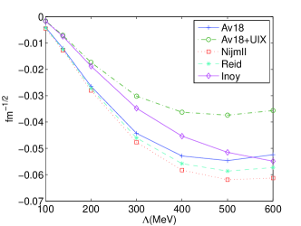
(a) $\mu^{2}\widetilde{\cal E}_{\frac{3}{2}(+)}$ for operator 1

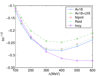
(b) $\mu^{2}\widetilde{\cal E}_{\frac{3}{2}(+)}$ for operator 9

Figure 1: Cutoff and strong model dependencies of $\mu^{2}\widetilde{\cal E}$ in $fm^{-\frac{1}{2}}$ for $\not{\pi}$EFT-I calculated with AV18, AV18+UIX, Nijmegen-II, INOY, and Reid strong potentials. The multiplier $\mu^{2}$ is used to absorb artificial cutoff dependence of $c_{n}$ coefficients.

As an example, let us consider the $\mu^{2}\widetilde{\cal E}_{\frac{3}{2}(+)}$ matrix elements as a function of a cutoff mass, which is calculated for operators 1 and 9 in the $\not{\pi}$EFT-I approach with different strong potentials (see Fig.1). The choice of these operators is related to their symmetry properties: the operator 1 has quantum numbers corresponding to pion-exchange while the operator 9 - to $\rho$-meson exchange. It should be noted that since we use the same scalar functions both for the $\not{\pi}$EFT-I and for the DDH-II schemes of calculations, we can apply the result of this analysis also to the calculations in the DDH-II scheme. Once again one observes rather strong dependence on the choice of a strong potential and on a cutoff mass parameter.

Analyzing results of Fig.1 from the point of view of the DDH approach, where the matrix element for the operator 1 at $\mu=m_{\pi}$ corresponds to the pion-meson exchange and the matrix element for the operator 9 at $\mu=m_{\rho}$ corresponds to the rho-meson exchange, one can see a large strong potential model dependence for heavy meson exchange. This dependence indicates the importance of the inclusion of 3-body strong potentials. Unfortunately, most calculations of PV effects in nuclear physics with the DDH potential do not include strong 3-body forces, which could be a possible source for the existing discrepancy Holstein (2005b) in the analysis of PV effects.

On the other hand, from the point of view of $\not{\pi}$EFT, the reasonable cutoff mass scale cannot exceed the value of the pion mass, where the dependance on strong interaction potential is small. Since the cutoff in EFT could be considered as a measure of our knowledge of short range physics, increasing the cutoff parameter implies stronger dependence on the short distance details. Fig.1 shows that by lowering the cutoff, one can diminish the strong potential model dependence. This is because by lowering of the cutoff parameter, we are effectively switching to the regime where the theory becomes sensitive only to a long range part of the interaction. Then, one can expect a smaller model dependence when the cutoff parameter is low, because all strong potentials have a similar long range behavior. Therefore, Fig.1 is consistent with the basic principle of the EFT and shows that the hybrid method works well.

The remaining weak dependence on strong interaction model at $\mu\simeq m_{\pi}$ scale could be related both to short and to long range parts of the potentials. If they are the remainder of the short distance part of wave function, the difference should be absorbed by LECs. On contrary the difference in the long range part of the wave function can not be removed by the renormalization of LECs in the hybrid method. However, as demonstrated in Song et al. (2009), this long range part difference is governed by strong interaction observables and should be easily treated by analyzing the correlation between matrix elements and effective range parameters.

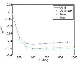
(a) $\Lambda^{2}\widetilde{\cal E}_{\frac{1}{2},(+)}$ for op1

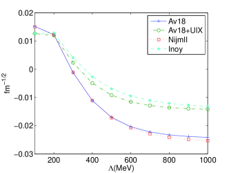
(b) $\Lambda^{2}\widetilde{\cal E}_{\frac{3}{2},(+)}$ for op1

Figure 2: Cutoff and strong model dependencies of $\Lambda^{2}\widetilde{\cal E}$ in $fm^{-\frac{1}{2}}$ for $\pi$EFT-I. The multiplier $\Lambda^{2}$ is used to absorb artificial cutoff dependence of $c_{n}$ coefficients.

To analyze the possible model dependence for the pionful EFT approach, let us consider a contribution of operator 1 to $\Lambda^{2}\widetilde{\cal E}_{\frac{1}{2},(-)}$ and to $\Lambda^{2}\widetilde{\cal E}_{\frac{3}{2},(+)}$ calculated in $\pi$EFT-I approach (see Fig. 2). In $\pi$EFT, the physical range for cutoff mass scale parameter $\Lambda$ is about $500<\Lambda<800$ MeV. One can observe a rather important dependence on strong potential model in this region. We cannot discern long range from short range model dependency unless all LECs are determined. However, a smaller range of the variation of matrix elements for different strong potentials at the pion mass scale indicates that the contribution of the long range part of strong potentials to the region of the interest ($500<\Lambda<800$ MeV) is small. This means that the large model dependence in this range ($500<\Lambda<800$ MeV) is due to short range part of the wave function, therefore this cutoff and model dependence should be absorbed by higher order contact terms.

Though the general behavior of the matrix elements are consistent with the expectations of EFT, the 3-body system is rather complicated one to see the direct relations between the 2-body PV potential and 3-body PV matrix elements. Therefore, it is useful to re-analyze the two-body n-p capture process, for which the large model dependence for a circular polarization of photons, $P^{\gamma}$, was reported in Schiavilla et al. (2004).

III.5 Two body radiative capture($n+p\to d+\gamma$)

Parity violating asymmetry of photons for polarized neutron capture on protons and and their circular polarization for the case of unpolarized neutron capture can be written as

$$a^{\gamma} = \frac{-\sqrt{2}{\rm Re}\{M_{1}^{*}(^{1}S_{0})E_{1}(^{3}S_{1})\}}{|M_{1}(^{1}S_{0})|^{2}}$$ (33)

$$P^{\gamma} = \frac{2{\rm Re}[M_{1}(^{1}S_{0})E^{*}_{1}(^{1}S_{0})]}{|M_{1}(^{1}S_{0})|^{2}}.$$ (34)

Here, we neglected $M_{1}(^{3}S_{1})$, and $E_{1}(^{1}P_{1}\leftarrow^{3}S_{1})$ amplitudes. The $E_{1}(^{3}S_{1})$ amplitude is a sum of amplitudes with contributions from parity violating bound state wave function and from parity violating scattering wave $(^{3}P_{1}\leftarrow^{3}S_{1})$. Since $M_{1}(^{3}S_{1})$ amplitude is suppressed, one can consider only $E_{1}(^{1}S_{0})$ contribution to the $P^{\gamma}$, which is dominated by $\rho$ and $\omega$ meson exchanges in the DDH formalism. (The $a_{n}^{\gamma}$ is dominated by one-pion exchange.)

The parity conserving M1 amplitude can be written as

$$M1(^{1}S_{0})=i\frac{\omega\mu_{N}}{\sqrt{6\pi}\sqrt{4\pi}}\widetilde{\cal M}=i\frac{\omega\mu_{N}}{\sqrt{6\pi}\sqrt{4\pi}}\left(\sqrt{4\pi}\sqrt{3}(393.06)\ fm^{\frac{3}{2}}\right).$$ (35)

Then, PV observables can be written as

$$a_{n}^{\gamma} = \sum_{m}\left(\frac{c_{m}}{\mu_{N}}\right)(-\sqrt{8\pi})\frac{\widetilde{\cal E}^{(m)}(^{3}S_{1})}{\widetilde{\cal M}(^{1}S_{0})},$$

$$P^{\gamma} = \sum_{m}\left(\frac{c_{m}}{\mu_{N}}\right)(-2\sqrt{4\pi})\frac{\widetilde{\cal E}^{(m)}(^{1}S_{0})}{\widetilde{\cal M}(^{1}S_{0})}.$$ (36)

Using strong AV18 and weak DDH-II potentials, one can obtain

$$a^{\gamma}_{n} = 0.15h^{1}_{\pi}+0.00137h^{1}_{\rho}-0.00405h^{1}_{\omega}-0.00137h^{\prime 1}_{\rho},$$ (37)

$$P^{\gamma} = -0.0104h^{0}_{\rho}-0.00817h^{2}_{\rho}+0.0111h^{0}_{\omega}.$$ (38)

Table 13: Two-body Parity violating observables for potential models with DDH-best parameter values and Bowman’s 4-parameter fits.

models	${a}^{\gamma}_{n}$		$P_{\gamma}$
	DDH-best	4-para. fit	DDH-best	4-para. fit
AV18 +DDH-I	$5.25\times 10^{-8}$	$-4.91\times 10^{-9}$	$6.94\times 10^{-9}$	$4.76\times 10^{-9}$
AV18 +DDH-II	$5.29\times 10^{-8}$	$-4.81\times 10^{-9}$	$1.76\times 10^{-8}$	$3.01\times 10^{-8}$
NijmII+DDH-II	$5.37\times 10^{-8}$	$-4.99\times 10^{-9}$	$2.61\times 10^{-8}$	$6.41\times 10^{-8}$
Reid+DDH-II	$5.33\times 10^{-8}$	$-4.85\times 10^{-9}$	$2.65\times 10^{-8}$	$4.68\times 10^{-8}$
INOY+DDH-II	$5.60\times 10^{-8}$	$-3.94\times 10^{-9}$	$2.55\times 10^{-7}$	$9.68\times 10^{-7}$

The calculated values of PV observables for different sets of strong potentials and different choices of DDH coupling constants are summarized in Table 13. One can see that the circular polarization $P^{\gamma}$, being dominated by heavy meson exchange, shows large model dependence in agreement with the analysis of n-d case.

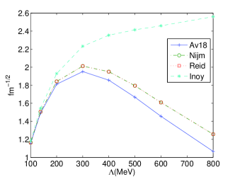
(a) $\mu^{2}\widetilde{\cal E}_{1,(+)}$ of operator 1

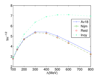
(b) $\mu^{2}\widetilde{\cal E}_{0,(-)}$ of operator 9

Figure 3: PV transition amplitudes $\mu^{2}\widetilde{\cal E}_{J,(+)}$ in $fm^{-\frac{1}{2}}$ for AV18 strong potential and PV $\not{\pi}EFT$-I potential.

The cutoff and model dependence of the transition matrix elements calculated for operators 1 and 9 using $\not{\pi}$EFT-I approach, shown in Figure 3, remind the corresponding cutoff and model dependencies for the n-d capture process. One can see that the model dependence is more pronounced at the scale of $\rho$ or $\omega$ meson masses in comparison to the pion mass region scale. This is also consistent with the statement given for the hybrid approach that one can regularize the short distance contributions by introducing a cutoff parameter and, as a consequence, reduce the uncertainty related to the short range interactions. This indicates that the possible reason for model and cutoff dependencies in 3-body (n-d capture) process has the same origin as those in 2-body case, and it can be treated regularly in the hybrid approach.

For the completeness of the analysis, we present contributions of different PV operators to PV observables calculated in $\not{\pi}$EFT and $\pi$EFT approaches with the AV18 potential (see tables 14 and 15, correspondingly). The large difference between matrix elements with pionless and pionful PV potentials could be explained by different scales of cutoff parameters, and the comparison of th e results obtained from these two approaches could be done only after the renormalization of low energy constants.

Table 14: Two body Parity violating observables for AV18 and $\not{\pi}$EFT potential at $\mu=138$ MeV.

	$\not{\pi}$EFT-I		$\not{\pi}$EFT-II
n	$\mu^{2}{a}_{n}^{(n)}$	$\mu^{2}{P}^{(n)}_{\gamma}$	$\mu^{2}{a}_{n}^{(n)}$	$\mu^{2}{P}^{(n)}_{\gamma}$
1	$6.02\times 10^{-3}$	0	$1.36\times 10^{-2}$	0
6	0	$2.48\times 10^{-2}$	0	$5.71\times 10^{-2}$
8	0	$1.99\times 10^{-2}$	0	$1.78\times 10^{-2}$
9	0	$-2.17\times 10^{-2}$	0	$-5.97\times 10^{-2}$

Table 15: Two body Parity violating observables for AV18 and ${\pi}$EFT potential at $\Lambda=600$ MeV. Only non-vanishing matrix elements are shown.

	$\pi$EFT-I	$\pi$EFT-II		$\pi$EFT-I	$\pi$EFT-II
op	$a_{n}^{\gamma(n)}$	$a_{n}^{\gamma(n)}$	op	$P_{\gamma}^{(n)}$	$P_{\gamma}^{(n)}$
1	$1.22\times 10^{-2}$	$7.14\times 10^{-3}$	6	$3.05\times 10^{-3}$	$2.01\times 10^{-3}$
13	$1.11\times 10^{-3}$	$5.59\times 10^{-4}$	8	$2.70\times 10^{-3}$	$1.80\times 10^{-3}$
14	$1.33\times 10^{-3}$	$7.41\times 10^{-4}$	9	$-4.13\times 10^{-3}$	$-2.36\times 10^{-3}$
15	$2.17\times 10^{-3}$	$1.00\times 10^{-3}$

IV Conclusion

PV effects in neutron-deuteron radiative capture are calculated for DDH-type and EFT-type, pionless and pionful, weak interaction potentials. Three-body problem was solved using Faddeev equations in configuration space, also by varying the strong interaction part of the Hamiltonian. Number of different phenomenological strong potentials has been tested, including AV18 NN interaction in conjunction with UIX 3-nucleon force. The analysis of the obtained results shows that the values of PV amplitudes depend both on the choice of the weak as well as strong interaction model. We demonstrated that this dependence has the expected behavior in the framework of the standard pionless and pionful EFT approaches. Therefore, this dependence is expected to be absorbed by LECs. Nevertheless, in order to obtain model independent EFT predictions for PV observables, one should perform all the calculations in a self-consistent way Gudkov and Song (2010). Using the “hybrid” approach we can minimize the model dependence, provided that all LECs are defined from the sufficiently large set of experimental data, which does not look practical in the nearest future.

For the case of the DDH approach, the observed model dependence indicates intrinsic difficulty in the description of nuclear PV effects and could be the reason for the observed discrepancies in the nuclear PV data analysis (see, for example Holstein (2009) and referencies therein). Thus, the DDH approach could be a reasonable approach for the parametrization and for the analysis of PV effects only if exactly the same strong and weak potentials are used in calculating all PV observables in all nuclei. However, the existing calculations of nuclear PV effects have been done using different potentials; therefore, strictly speaking, one cannot compare the existing results of these calculations among themselves. Further, most of the existing calculations do not include three body interaction which is shown to be important.

We would like to mention that the observed sensitivity of PV effects to short range parts of interactions could be used as a new method for the study of short ranges nuclear forces. Once the theory PV effects is well understood, or once we use exactly the same parametrization for weak interactions, PV effects can be used to probe short distance dynamics of different nuclear systems described by different strong potentials.

*

References

• Zhu et al. (2005) S.-L. Zhu, C. M. Maekawa, B. R. Holstein, M. J. Ramsey-Musolf, and U. van Kolck, Nucl. Phys. A748, 435 (2005).
• Holstein (2005a) B. Holstein, Neutrons and hadronic parity violation (2005a), proc. of Int. Workshop on Theoretical Problems in Fundamental Neutron Physics, October 14-15, 2005, Columbia, SC, eprint http://www.physics.sc.edu/TPFNP/Talks/Program.html.
• Desplanque (2005) B. Desplanque, Weak couplings: a few remarks (2005), proc. of Int. Workshop on Theoretical Problems in Fundamental Neutron Physics, October 14-15, 2005, Columbia, SC, eprint http://www.physics.sc.edu/TPFNP/Talks/Program.html.
• Ramsey-Musolf and Page (2006) M. J. Ramsey-Musolf and S. A. Page, Ann. Rev. Nucl. Part. Sci. 56, 1 (2006).
• Desplanques et al. (1980a) B. Desplanques, J. F. Donoghue, and B. R. Holstein, Annals of Physics 124, 449 (1980a).
• Liu (2007) C. P. Liu, Phys. Rev. C75, 065501 (2007).
• Girlanda (2008) L. Girlanda, Phys. Rev. C77, 067001 (2008), eprint 0804.0772.
• Phillips et al. (2009) D. R. Phillips, M. R. Schindler, and R. P. Springer, Nucl. Phys. A822, 1 (2009).
• Shin et al. (2010) J. W. Shin, S. Ando, and C. H. Hyun, Phys. Rev. C81, 055501 (2010).
• Schindler and Springer (2009) M. R. Schindler and R. P. Springer (2009), eprint 0907.5358.
• Sushkov and Flambaum (1982) O. P. Sushkov and V. V. Flambaum, Sov. Phys. Usp. 25, 1 (1982).
• Bunakov and Gudkov (1983) V. E. Bunakov and V. P. Gudkov, Nucl. Phys. A401, 93 (1983).
• Gudkov (1992) V. P. Gudkov, Phys. Rept. 212, 77 (1992).
• Schiavilla et al. (2008) R. Schiavilla, M. Viviani, L. Girlanda, A. Kievsky, and L. E. Marcucci, Phys. Rev. C78, 014002 (2008).
• Song et al. (2011a) Y.-H. Song, R. Lazauskas, and V. Gudkov, Phys.Rev. C83, 015501 (2011a), eprint 1011.2221.
• Moskalev (1969) A. Moskalev, Sov. J. of Nucl. Phys. 9, 99 (1969).
• E. Hadjimichael and Newton (1974) E. H. E. Hadjimichael and V. Newton, Nucl. Phys. A228, 1 (1974).
• McKellar (1974) B. H. McKellar, Phys.Rev. C9, 1790 (1974).
• Desplanques and Benayoun (1986) B. Desplanques and J. Benayoun, Nucl.Phys. A458, 689 (1986).
• Song et al. (2009) Y.-H. Song, R. Lazauskas, and T.-S. Park, Phys. Rev. C79, 064002 (2009).
• Pastore et al. (2009) S. Pastore, L. Girlanda, R. Schiavilla, M. Viviani, and R. B. Wiringa, Phys. Rev. C80, 034004 (2009).
• Song et al. (2007) Y.-H. Song, R. Lazauskas, T.-S. Park, and D.-P. Min, Phys. Lett. B656, 174 (2007).
• Lazauskas et al. (2009) R. Lazauskas, Y.-H. Song, and T.-S. Park (2009), eprint 0905.3119.
• Park et al. (2003) T. S. Park et al., Phys. Rev. C67, 055206 (2003).
• Girlanda et al. (2010) L. Girlanda et al. (2010), eprint 1008.0356.
• Song et al. (2011b) Y.-H. Song, R. Lazauskas, and V. Gudkov, Phys.Rev. C83, 065503 (2011b), eprint 1104.3051.
• Song et al. (2011c) Y.-H. Song, R. Lazauskas, and V. Gudkov, Phys.Rev. C84, 025501 (2011c), eprint 1105.1327.
• Griesshammer et al. (2012) H. W. Griesshammer, M. R. Schindler, and R. P. Springer, Eur.Phys.J. A48, 7 (2012), eprint 1109.5667.
• Desplanques et al. (1980b) B. Desplanques, J. F. Donoghue, and B. R. Holstein, Ann. Phys. 124, 449 (1980b), ISSN 0003-4916.
• Schiavilla et al. (2004) R. Schiavilla, J. Carlson, and M. W. Paris, Phys. Rev. C70, 044007 (2004).
• Hyun et al. (2007) C. Hyun, S. Ando, and B. Desplanques, Eur.Phys.J. A32, 513 (2007), eprint nucl-th/0609015.
• Faddeev (1961) L. D. Faddeev, Sov. Phys. JETP 12, 1014 (1961).
• Lazauskas (2003) R. Lazauskas (2003), universite Joseph Fourier, Grenoblex.
• Lazauskas (2009) R. Lazauskas, Few-Body Systems 46, 37 (2009), URL http://arxiv.org/abs/0808.1650.
• (35) J. D. Bowman, “Hadronic Weak Interaction”, INT Workshop on Electric Dipole Moments and CP Violations, March 19-23, 2007, eprint http://www.int.washington.edu/talks/WorkShops/$int\_07\_1$/.
• Holstein (2005b) B. R. Holstein, Fizika. B14, 165 (2005b), eprint nucl-th/0607038.
• Gudkov and Song (2010) V. Gudkov and Y.-H. Song, Phys. Rev. C82, 028502 (2010).
• Holstein (2009) B. R. Holstein, Eur. Phys. J. A41, 279 (2009).