Embedded Gaussian Unitary Ensembles with $U(\Omega)\otimes SU(r)$ Embedding generated by Random Two-body Interactions with $SU(r)$ Symmetry

Abstract

Following the earlier studies on embedded unitary ensembles generated by random two-body interactions [EGUE(2)] with spin $SU(2)$ and spin-isospin $SU(4)$ symmetries, developed is a general formulation, for deriving lower order moments of the one- and two-point correlation functions in eigenvalues, that is valid for any EGUE(2) and BEGUE(2) (’B’ stands for bosons) with $U(\Omega)\otimes SU(r)$ embedding and with two-body interactions preserving $SU(r)$ symmetry. Using this formulation with $r=1$, we recover the results derived by Asaga et al [Ann. Phys. (N.Y.) 297, 344 (2002)] for spinless boson systems. Going further, new results are obtained for $r=2$ (this corresponds to two species boson systems) and $r=3$ (this corresponds to spin 1 boson systems).

I Introduction

A long standing question for the embedded ensembles is about their analytical tractability. Amenability to mathematical treatment is one of the four conditions laid down by Dyson Dy-72 for the validity of a random matrix ensemble. Simplest of the two-body unitary ensemble is the embedded Gaussian unitary ensemble of two-body interactions [EGUE(2)] for spinless fermion systems. For $m$ fermions in $N$ sp states, the embedding is generated by the $SU(N)$ algebra and although this ensemble is known for many years, only recently Ko-05 , after the first indications implicit in Be-01b ; PlW , it is established that the $SU(N)$ Wigner-Racah algebra solves EGUE($2$) and also the more general EGUE($k$) [as well as EGOE($k)$]. These results, with $U(N)$ algebra, extended to BEGUE($k$) for spinless bosons in $N$ sp states (see Ko-05 ; Asa-02 ). For EGUE(2)-${\bf s}$ for fermions with spin and EGUE(2)-$SU(4)$ for fermions with Wigner’s spin-isospin $SU(4)$ symmetry, the embedding algebras, with $\Omega$ number of spatial degrees of freedom for a single fermion, are $U(\Omega)\otimes SU(2)$ and $U(\Omega)\otimes SU(4)$ respectively. It was shown in Ko-07 ; Ma-su4 that the Wigner-Racah algebra of these embedding algebras will allow one to obtain analytical results for the lower order moments of the one- and two-point correlation functions in eigenvalues. Similarly, following the recent work Ma-12 ; Ckmp-arx on BEGOEs, it is easy to recognize that the embedding algebras for BEGUE(2)-$F$ for two-species boson systems with $F$-spin and BEGUE(2)-$SU(3)$ for spin one boson systems are $U(\Omega)\otimes SU(2)$ and $U(\Omega)\otimes SU(3)$ respectively. The purpose of the present paper is to establish on one hand that the Wigner-Racah algebra of these embedding algebras solve the corresponding embedded unitary ensembles and on the other to generalize the formalism to any EGUE(2) with $U(\Omega)\otimes SU(r)$ embedding and generated by random two-body interaction with $SU(r)$ symmetry. Hereafter we call these ensembles EGUE(2)-$SU(r)$ and they apply to both fermion and boson systems.

In Section 2, given is the general formulation based on Wigner-Racah algebra for lower order moments of the one- and two-point functions in eigenvalues generated by EGUE(2)-$SU(r)$ ($r$ is any positive integer, $r\geq 1$). Sections 3, 4 and 5 give analytical results for boson systems with $r=1$, $r=2$ and $r=3$ respectively. In addition, some numerical results for lower order correlations generated by these ensembles are also given in Section 5. Finally, Section 6 gives concluding remarks.

II EGUE(2)-$SU(r)$ ensembles: General formulation

Consider a system of $m$ fermions or bosons in $\Omega$ number of sp levels each $r$-fold degenerate. Then the SGA is $U(r\Omega)$ and it is possible to consider $U(r\Omega)\supset U(\Omega)\otimes SU(r)$ algebra. Now, for random two-body Hamiltonians preserving $SU(r)$ symmetry, one can introduce embedded GUE with $U(\Omega)\otimes SU(r)$ embedding and this ensemble is called EGUE(2)-$SU(r)$. Ensembles with $r=2,4$ for fermions correspond to fermions with spin and spin-isospin $SU(4)$ symmetry. Similarly, for bosons $r=2,3$ are of interest. Also $r=1$ gives back EGUE(2) and BEGUE(2) both. It is important to note that the distinction between fermions and bosons is in the $U(\Omega)$ irreps that need to be considered. Now we will give a formulation in terms of $SU(\Omega)$ Wigner-Racah algebra (the $SU(r)$ algebra involved will be simple as $H$ has $SU(r)$ symmetry) that is valid for any $r$. The discussion in the remaining part of this Section is essentially from Ma-su4 but it is repeated briefly not only for completeness but also to generalize it to any $r$ and also to bosons systems (in Ma-su4 , fermions with $r=4$ is used).

Let us begin with normalized two-particle states $\left.\left|f_{2}F_{2};v_{2}\beta_{2}\right.\right\rangle$ where the $U(r)$ irreps $F_{2}=\{1^{2}\}$ and $\{2\}$ and the corresponding $U(\Omega)$ irreps $f_{2}$ are $\{2\}$ (symmetric) and $\{1^{2}\}$ (antisymmetric) respectively for fermions and $\{1^{2}\}$ (antisymmetric) and $\{2\}$ (symmetric) respectively for bosons. Similarly $v_{2}$ are additional quantum numbers that belong to $f_{2}$ and $\beta_{2}$ belong to $F_{2}$. As $f_{2}$ uniquely defines $F_{2}$, from now on we will drop $F_{2}$ unless it is explicitly needed and also we will use the $f_{2}\leftrightarrow F_{2}$ equivalence whenever needed. With $A^{\dagger}(f_{2}v_{2}\beta_{2})$ and $A(f_{2}v_{2}\beta_{2})$ denoting creation and annihilation operators for the normalized two particle states, a general two-body Hamiltonian operator ${\widehat{H}}$ preserving $SU(r)$ symmetry can be written as

$${\widehat{H}}={\widehat{H}}_{\{2\}}+{\widehat{H}}_{\{1^{2}\}}=\displaystyle\sum_{f_{2},v_{2}^{i},v_{2}^{f},\beta_{2};f_{2}=\{2\},\{1^{2}\}}\;H_{f_{2}v_{2}^{i}v_{2}^{f}}(2)\;A^{\dagger}(f_{2}v^{f}_{2}\beta_{2})\,A(f_{2}v^{i}_{2}\beta_{2})\;.$$ (1)

In Eq. (1), $H_{f_{2}v_{2}^{i}v_{2}^{f}}(2)=\left\langle f_{2}v^{f}_{2}\beta_{2}\mid H\mid f_{2}v^{i}_{2}\beta_{2}\right\rangle$ independent of the $\beta_{2}$’s. The uniform summation over $\beta_{2}$ in Eq. (1) ensures that ${\widehat{H}}$ is $SU(r)$ scalar and therefore it will not connect states with different $f_{2}$’s. However, ${\widehat{H}}$ is not a $SU(r)$ invariant operator. Just as the two particle states, we can denote the $m$ particle states by $\left|f_{m}v_{m}^{f}\beta_{m}^{F}\right\rangle$; $F_{m}=\widetilde{f}_{m}$ for fermions and $F_{m}=f_{m}$ for bosons. Action of ${\widehat{H}}$ on these states generates states that are degenerate with respect to $\beta_{m}^{F}$ but not $v_{m}^{f}$. Therefore for a given $f_{m}$, there will be $d_{\Omega}(f_{m})$ number of levels each with $d_{r}(\tilde{f}_{m})$ number of degenerate states. Formula for the dimension $d_{\Omega}(f_{m})$ is Wy-70 ,

$$d_{\Omega}(f_{m})=\displaystyle\prod_{i<j=1}^{\Omega}\displaystyle\frac{f_{i}-f_{j}+j-i}{j-i}\;,$$ (2)

where, $f_{m}=\{f_{1},f_{2},\ldots\}$. Equation (2) also gives $d_{r}(F_{m})$ with the product ranging from $i=1$ to $r$ and replacing $f_{i}$ by $F_{i}$. As ${\widehat{H}}$ is a $SU(r)$ scalar, the $m$ particle $H$ matrix will be a direct sum of matrices with each of them labeled by the $f_{m}$’s with dimension $d_{\Omega}(f_{m})$. Thus

$$H(m)=\displaystyle\sum_{f_{m}}\;H_{f_{m}}(m)\oplus\;.$$ (3)

It should be noted that the matrix elements of $H_{f_{m}}(m)$ matrices receive contributions from both $H_{\{2\}}(2)$ and $H_{\{1^{2}\}}(2)$.

Embedded random matrix ensemble EGUE(2)-$SU(r)$ for a $m$ fermion or boson system with a fixed $f_{m}$, i.e. $\{H_{f_{m}}(m)\}$, is generated by the ensemble of $H$ operators given in Eq. (1) with $H_{\{2\}}(2)$ and $H_{\{1^{2}\}}(2)$ matrices replaced by independent GUE ensembles of random matrices,

$$\{H(2)\}=\{H_{\{2\}}(2)\}_{GUE}\oplus\{H_{\{1^{2}\}}(2)\}_{GUE}\;.$$ (4)

In Eq. (4), $\{--\}$ denotes ensemble. Random variables defining the real and imaginary parts of the matrix elements of $H_{f_{2}}(2)$ are independent Gaussian variables with zero center and variance given by (with bar representing ensemble average),

$$\overline{H_{f_{2}v_{2}^{1}v_{2}^{2}}(2)\;H_{f_{2}^{\prime}v_{2}^{3}v_{2}^{4}}(2)}=\delta_{f_{2}f_{2}^{\prime}}\delta_{v_{2}^{1}v_{2}^{4}}\delta_{v_{2}^{2}v_{2}^{3}}\,(\lambda_{f_{2}})^{2}\;.$$ (5)

Also, the independence of the $\{H_{\{2\}}(2)\}$ and $\{H_{\{1^{2}\}}(2)\}$ GUE ensembles imply,

$$\overline{\left[H_{\{2\}v_{2}^{1}v_{2}^{2}}(2)\right]^{P}\;\left[H_{\{1^{2}\}v_{2}^{3}v_{2}^{4}}(2)\right]^{Q}}=\left\{\;\overline{\left[H_{\{2\}v_{2}^{1}v_{2}^{2}}(2)\right]^{P}}\;\right\}\;\;\left\{\;\overline{\left[H_{\{1^{2}\}v_{2}^{3}v_{2}^{4}}(2)\right]^{Q}}\;\right\}$$ (6)

for $P$ and $Q$ even and zero otherwise. Action of ${\widehat{H}}$ defined by Eq. (1) on $m$ particle basis states with a fixed $f_{m}$, along with Eqs. (5)-(6) generates EGUE(2)-$SU(r)$ ensemble $\{H_{f_{m}}(m)\}$; it is labeled by the $U(\Omega)$ irrep $f_{m}$ with matrix dimension $d_{\Omega}(f_{m})$.

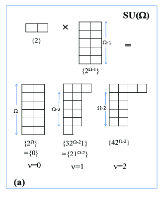
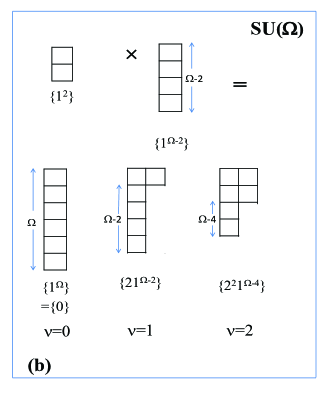
Figure 1: Young tableaux for the tensorial parts of a two-body Hamiltonian with respect to $SU(\Omega)$ algebra. Young tableaux for various (a) tensorial parts with respect to $SU(\Omega)$ for the $f_{2}=\{2\}$ part of $H$; (b) tensorial parts with respect to $SU(\Omega)$ for the $f_{2}=\{1^{2}\}$ part of $H$.

As shown in Ko-05 ; Ko-07 ; Ma-su4 , tensorial decomposition of ${\widehat{H}}$ with respect to the embedding algebra $U(\Omega)\otimes SU(r)$ plays a crucial role in generating analytical results; as before $U(\Omega)$ and $SU(\Omega)$ are used interchangeably. As ${\widehat{H}}$ preserves $SU(r)$, it transforms as the irrep $\{0\}$ with respect to the $SU(r)$ algebra. However with respect to $SU(\Omega)$, the tensorial characters, in Young tableaux notation, for $f_{2}=\{2\}$ are ${\mbox{\boldmath$F$}}_{\nu}=\{0\}$, $\{21^{\Omega-2}\}$ and $\{42^{\Omega-2}\}$ with $\nu=0,1$ and 2 respectively. Similarly for $f_{2}=\{1^{2}\}$ they are ${\mbox{\boldmath$F$}}_{\nu}=\{0\}$, $\{21^{\Omega-2}\}$ and $\{2^{2}1^{\Omega-4}\}$ with $\nu=0,1,2$ respectively. Note that ${\mbox{\boldmath$F$}}_{\nu}=f_{2}\times\overline{f_{2}}$ where $\overline{f_{2}}$ is the irrep conjugate to $f_{2}$ and the $\times$ denotes Kronecker product. Given a $U(\Omega)$ irrep $\{f\}=\{f_{1},f_{2},\ldots,f_{\Omega}\}$, we have $\overline{f}=\{f_{1}-f_{\Omega},f_{1}-f_{\Omega-1},\ldots,f_{1}-f_{2},0\}$. Young tableaux for the $F_{\nu}$’s are shown in Fig. 1. Now, we can define unitary tensors $B$’s that are scalars in $SU(r)$ space,

$$\begin{array}[]{rcl}B(f_{2}{\mbox{\boldmath$F$}}_{\nu}\omega_{\nu})&=&\displaystyle\sum_{v_{2}^{i},v_{2}^{f},\beta_{2}}\,A^{\dagger}(f_{2}v^{f}_{2}\beta_{2})\,A(f_{2}v^{i}_{2}\beta_{2})\,\left\langle f_{2}v_{2}^{f}\;\overline{f_{2}}\,\overline{v_{2}^{i}}\mid{\mbox{\boldmath$F$}}_{\nu}\omega_{\nu}\right\rangle\\ &\times&\left\langle F_{2}\beta_{2}\;\overline{F_{2}}\,\overline{\beta_{2}}\mid 00\right\rangle\;.\end{array}$$ (7)

In Eq. (7), $\left\langle f_{2}---\right\rangle$ are $SU(\Omega)$ Wigner coefficients and $\left\langle F_{2}---\right\rangle$ are $SU(r)$ Wigner coefficients. The expansion of ${\widehat{H}}$ in terms of $B$’s is,

$${\widehat{H}}=\displaystyle\sum_{f_{2},{\mbox{\boldmath$F$}}_{\nu},\;\omega_{\nu}}\;W(f_{2}{\mbox{\boldmath$F$}}_{\nu}\omega_{\nu})\,B(f_{2}{\mbox{\boldmath$F$}}_{\nu}\omega_{\nu})\;.$$ (8)

The expansion coefficients $W$’s follow from the orthogonality of the tensors $B$’s with respect to the traces over fixed $f_{2}$ spaces. Then we have the most important relation needed for all the results given ahead,

$$\overline{W(f_{2}{\mbox{\boldmath$F$}}_{\nu}\omega_{\nu})W(f^{\prime}_{2}{\mbox{\boldmath$F$}}^{\prime}_{\nu}\omega^{\prime}_{\nu})}=\delta_{f_{2}f^{\prime}_{2}}\delta_{{\mbox{\boldmath$F$}}_{\nu}{\mbox{\boldmath$F$}}^{\prime}_{\nu}}\delta_{\omega_{\nu}\omega^{\prime}_{\nu}}\,(\lambda_{f_{2}})^{2}d_{r}(F_{2})\,.$$ (9)

This is derived starting with Eq. (8) and using Eqs. (4)-(7) along with the sum rules for Wigner coefficients appearing in Eq. (7).

Turning to $m$ particle $H$ matrix elements, first we denote the $U(\Omega)$ and $U(r)$ irreps by $f_{m}$ and $F_{m}$ respectively. Correlations generated by EGUE(2)-$SU(r)$ between states with $(m,f_{m})$ and $(m^{\prime},f_{m^{\prime}})$ follow from the covariance between the $m$-particle matrix elements of $H$. Now using Eqs. (8) and (9) along with the Wigner-Eckart theorem applied using $SU(\Omega)\otimes SU(r)$ Wigner-Racah algebra (see for example He-74a ) will give

$$\begin{array}[]{l}\overline{H_{f_{m}v_{m}^{i}v_{m}^{f}}\,H_{f_{m^{\prime}}v_{m^{\prime}}^{i}v_{m^{\prime}}^{f}}}\\ \\ =\overline{\left\langle f_{m}F_{m}v_{m}^{f}\beta\mid H\mid f_{m}F_{m}v_{m}^{i}\beta\right\rangle\left\langle f_{m^{\prime}}F_{m^{\prime}}v_{m^{\prime}}^{f}\beta^{\prime}\mid H\mid f_{m^{\prime}}F_{m^{\prime}}v_{m^{\prime}}^{i}\beta^{\prime}\right\rangle}\\ \\ =\displaystyle\sum_{f_{2},{\mbox{\boldmath$F$}}_{\nu},\;\omega_{\nu}}\;\displaystyle\frac{(\lambda_{f_{2}})^{2}}{d_{\Omega}(f_{2})}\;\displaystyle\sum_{\rho,\rho^{\prime}}\;\left\langle f_{m}\mid\mid\mid B(f_{2}{\mbox{\boldmath$F$}}_{\nu})\mid\mid\mid f_{m}\right\rangle_{\rho}\;\left\langle f_{m^{\prime}}\mid\mid\mid B(f_{2}{\mbox{\boldmath$F$}}_{\nu})\mid\mid\mid f_{m^{\prime}}\right\rangle_{\rho^{\prime}}\\ \\ \times\left\langle f_{m}v_{m}^{i}\;{\mbox{\boldmath$F$}}_{\nu}\omega_{\nu}\mid f_{m}v_{m}^{f}\right\rangle_{\rho}\;\left\langle f_{m^{\prime}}v_{m^{\prime}}^{i}\;{\mbox{\boldmath$F$}}_{\nu}\omega_{\nu}\mid f_{m^{\prime}}v_{m^{\prime}}^{f}\right\rangle_{\rho^{\prime}}\,;\\ \\ \left\langle f_{m}\mid\mid\mid B(f_{2}{\mbox{\boldmath$F$}}_{\nu})\mid\mid\mid f_{m}\right\rangle_{\rho}\,=\displaystyle\sum_{f_{m-2}}\;F(m)\,\displaystyle\frac{{\cal N}_{f_{m-2}}}{{\cal N}_{f_{m}}}\;\displaystyle\frac{U(f_{m}\overline{f_{2}}f_{m}f_{2};f_{m-2}{\mbox{\boldmath$F$}}_{\nu})_{\rho}}{U(f_{m}\overline{f_{2}}f_{m}f_{2};f_{m-2}\{0\})}\;.\end{array}$$ (10)

Here the summation in the last equality is over the multiplicity index $\rho$ and this arises as $f_{m}\times{\mbox{\boldmath$F$}}_{\nu}$ gives in general more than once the irrep $f_{m}$. In Eq. (10),

$$F(m)=-m(m-1)/2\;,$$ (11)

$d_{\Omega}(f_{m})$ is given by Eq. (2) and $\left\langle\ldots\right\rangle$ and $U(\ldots)$ are $SU(\Omega)$ Wigner and Racah coefficients respectively. Similarly, ${\cal N}_{f_{m}}$ is dimension with respect to the $S_{m}$ group Wy-70 ,

$${\cal N}_{f_{m}}=\displaystyle\frac{m!\displaystyle\prod_{i<k=1}^{p}(\ell_{i}-\ell_{k})}{\ell_{1}!\;\ell_{2}!\ldots\ell_{p}!}\;;\;\;\;\;\ell_{i}=f_{i}+p-i\;.$$ (12)

Note that $p$ denotes total number of rows in the Young tableaux for $f_{m}$.

Lower order cross correlations between states with different $(m,f_{m})$ are given by the normalized bivariate moments $\Sigma_{PQ}\left(m,f_{m}:m^{\prime},f_{m^{\prime}}\right)$, $P=Q=1,2$ of the two-point function $S^{\rho}$ where, with $\rho^{m,f_{m}}(E)$ defining fixed-$(m,f_{m})$ density of states,

$$\begin{array}[]{l}S^{mf_{m}:m^{\prime}f_{m^{\prime}}}(E,E^{\prime})=\overline{\rho^{m,f_{m}}(E)\rho^{m^{\prime},f_{m^{\prime}}}(E^{\prime})}-\overline{\rho^{m,f_{m}}(E)}\;\;\overline{\rho^{m^{\prime},f_{m^{\prime}}}(E^{\prime})}\;\;;\\ \\ \Sigma_{11}\left({m,f_{m}}:{m^{\prime},f_{m^{\prime}}}\right)=\overline{\left\langle H\right\rangle^{m,f_{m}}\;\left\langle H\right\rangle^{m^{\prime},f_{m^{\prime}}}}/\displaystyle\sqrt{\,\overline{\left\langle H^{2}\right\rangle^{m,f_{m}}}\;\overline{\left\langle H^{2}\right\rangle^{m^{\prime},f_{m^{\prime}}}}}\;,\\ \\ {\Sigma}_{22}\left({m,f_{m}}:{m^{\prime},f_{m^{\prime}}}\right)=\overline{\left\langle H^{2}\right\rangle^{m,f_{m}}\;\left\langle H^{2}\right\rangle^{m^{\prime},f_{m^{\prime}}}}/\left[\,\overline{\left\langle H^{2}\right\rangle^{m,f_{m}}}\;\overline{\left\langle H^{2}\right\rangle^{m^{\prime},f_{m^{\prime}}}}\,\right]-1\;.\end{array}$$ (13)

In Eq. (13), $\overline{\left\langle H^{2}\right\rangle^{m,f_{m}}}$ is the second moment (or variance) of the eigen value density $\overline{\rho^{m,f_{m}}(E)}$ and its centroid $\overline{\left\langle H\right\rangle^{m,f_{m}}}=0$ by definition. As $\left\langle H\right\rangle^{m,f_{m}}$ is the trace of $H$ (divided by dimensionality) in $(m,f_{m})$ space, only ${\mbox{\boldmath$F$}}_{\nu}=\{0\}$ will generate $\overline{\left\langle H\right\rangle^{m,f_{m}}\;\left\langle H\right\rangle^{m^{\prime},f_{m^{\prime}}}}$. Then trivially,

$$\begin{array}[]{rcl}\overline{\left\langle H\right\rangle^{m,f_{m}}\;\left\langle H\right\rangle^{m^{\prime},f_{m^{\prime}}}}&=&\displaystyle\sum_{f_{2}}\displaystyle\frac{\left(\lambda_{f_{2}}\right)^{2}}{d_{\Omega}(f_{2})}\;P^{f_{2}}(m,f_{m})\;P^{f_{2}}(m^{\prime},f_{m^{\prime}})\;;\\ \\ P^{f_{2}}(m,f_{m})&=&F(m)\displaystyle\sum_{f_{m-2}}\;\displaystyle\frac{{\cal N}_{f_{m-2}}}{{\cal N}_{f_{m}}}\;.\end{array}$$ (14)

Writing $\overline{\left\langle H^{2}\right\rangle^{m,f_{m}}}$ explicitly in terms of $m$ particle $H$ matrix elements,

$$\overline{\left\langle H^{2}\right\rangle^{m,f_{m}}}=[d(f_{m})]^{-1}\sum_{v_{m}^{1},v_{m}^{2}}\,\overline{H_{f_{m}v_{m}^{1}v_{m}^{2}}\,H_{f_{m}v_{m}^{2}v_{m}^{1}}}\;,$$

and applying Eq. (10) and the orthonormal properties of the $SU(\Omega)$ Wigner coefficients lead to

$$\overline{\left\langle H^{2}\right\rangle^{m,f_{m}}}=\displaystyle\sum_{f_{2}}\displaystyle\frac{(\lambda_{f_{2}})^{2}}{d_{\Omega}(f_{2})}\displaystyle\sum_{\nu=0,1,2}{\cal Q}^{\nu}(f_{2}:m,f_{m})$$ (15)

where

$${\cal Q}^{\nu}(f_{2}:m,f_{m})=\left[F(m)\right]^{2}\displaystyle\sum_{f_{m-2},f^{\prime}_{m-2}}\displaystyle\frac{{\cal N}_{f_{m-2}}}{{\cal N}_{f_{m}}}\displaystyle\frac{{\cal N}_{f^{\prime}_{m-2}}}{{\cal N}_{f_{m}}}X_{UU}(f_{2};f_{m-2},f^{\prime}_{m-2};{\mbox{\boldmath$F$}}_{\nu})\;.$$ (16)

The $X_{UU}$ function involves $SU(\Omega)$ Racah coefficients,

$$\begin{array}[]{l}X_{UU}(f_{2};f_{m-2},f^{\prime}_{m-2};{\mbox{\boldmath$F$}}_{\nu})=\\ \displaystyle\sum_{\rho}\displaystyle\frac{U(f_{m},\overline{f_{2}},f_{m},f_{2};f_{m-2},{\mbox{\boldmath$F$}}_{\nu})_{\rho}U(f_{m},\overline{f_{2}},f_{m},f_{2};f^{\prime}_{m-2},{\mbox{\boldmath$F$}}_{\nu})_{\rho}}{U(f_{m},\overline{f_{2}},f_{m},f_{2};f_{m-2},\{0\})U(f_{m},\overline{f_{2}},f_{m},f_{2};f^{\prime}_{m-2},\{0\})}\;.\end{array}$$ (17)

Summation over the multiplicity index $\rho$ in Eq. (17) arises naturally in applications to physical problems as all the physically relevant results should be independent of $\rho$ which is a label for equivalent $SU(\Omega)$ irreps. It is easy to see that,

$${\cal Q}^{\nu=0}(f_{2}:m,f_{m})=\left[P^{f_{2}}(m,f_{m})\right]^{2}\;.$$ (18)

Eqs. (14)-(16) and Table 4 of Ma-su4 will allow us to calculate covariances ${\Sigma}_{11}$ in energy centroids; Table 4 of Ma-su4 is a simplified version of the tables in He-74 . For the covariances ${\Sigma}_{22}$ in spectral variances, the formula is Ma-su4

$$\begin{array}[]{l}{\Sigma}_{22}(m,f_{m};m^{\prime},f_{m^{\prime}})=\displaystyle\frac{X_{\{2\}}+X_{\{1^{2}\}}+4X_{\{1^{2}\}\{2\}}}{\overline{\left\langle H^{2}\right\rangle^{m,f_{m}}}\;\overline{\left\langle H^{2}\right\rangle^{m^{\prime},f_{m^{\prime}}}}}\;;\\ X_{f_{2}}=\displaystyle\frac{2(\lambda_{f_{2}})^{4}}{\left[d_{\Omega}(f_{2})\right]^{2}}\displaystyle\sum_{\nu=0,1,2}\left[d_{\Omega}({\mbox{\boldmath$F$}}_{\nu})\right]^{-1}{\cal Q}^{\nu}(f_{2}:m,f_{m}){\cal Q}^{\nu}(f_{2}:m^{\prime},f_{m^{\prime}})\;,\\ X_{\{1^{2}\}\{2\}}=\displaystyle\frac{\lambda^{2}_{\{2\}}\lambda^{2}_{\{1^{2}\}}}{d(\{2\})d(\{1^{2}\})}\displaystyle\sum_{\nu=0,1}\left[d_{\Omega}({\mbox{\boldmath$F$}}_{\nu})\right]^{-1}{\cal R}^{\nu}(m,f_{m})\;{\cal R}^{\nu}(m^{\prime},f_{m^{\prime}})\;.\end{array}$$ (19)

Here $d_{\Omega}({\mbox{\boldmath$F$}}_{\nu})$ is the dimension of the irrep ${\mbox{\boldmath$F$}}_{\nu}$, and we have $d_{\Omega}(\{0\})=1$, $d_{\Omega}(\{2,1^{\Omega-2}\})=\Omega^{2}-1$, $d_{\Omega}(\{4,2^{\Omega-2}\})=\Omega^{2}(\Omega+3)(\Omega-1)/4$, and $d_{\Omega}(\{2^{2},1^{\Omega-4}\})=\Omega^{2}(\Omega-3)(\Omega+1)/4$. Note that ${\cal Q}^{\nu}(f_{2}:m,f_{m})$ are defined in Eq. (16). The functions $R^{\nu}(m,f_{m})$ also involve $SU(\Omega)$ $U$-coefficients,

$$\begin{array}[]{l}R^{\nu}(m,f_{m})=\left[F(m)\right]^{2}\displaystyle\sum_{f_{m-2},f^{\prime}_{m-2}}\displaystyle\frac{{\cal N}_{f_{m-2}}}{{\cal N}_{f_{m}}}\displaystyle\frac{{\cal N}_{f_{m-2}^{\prime}}}{{\cal N}_{f_{m}}}Y_{UU}(f_{m-2},f^{\prime}_{m-2};{\mbox{\boldmath$F$}}_{\nu})\;;\\ Y_{UU}(f_{m-2},f^{\prime}_{m-2};{\mbox{\boldmath$F$}}_{\nu})=\\ \displaystyle\sum_{\rho}\displaystyle\frac{U(f_{m},\{1^{\Omega-2}\},f_{m},\{1^{2}\};f_{m-2},{\mbox{\boldmath$F$}}_{\nu})_{\rho}\,U(f_{m},\{2^{\Omega-1}\},f_{m},\{2\};f_{m-2}^{\prime},{\mbox{\boldmath$F$}}_{\nu})_{\rho}}{U(f_{m},\{1^{\Omega-2}\},f_{m},\{1^{2}\};f_{m-2},\{0\})\,U(f_{m},\{2^{\Omega-1}\},f_{m},\{2\};f_{m-2}^{\prime},\{0\})}\;.\end{array}$$ (20)

In $Y_{UU}(f_{m-2},f^{\prime}_{m-2};{\mbox{\boldmath$F$}}_{\nu})$, $f_{m-2}$ comes from $f_{m}\otimes\{1^{\Omega-2}\}$ and $f^{\prime}_{m-2}$ comes from $f_{m}\otimes\{2^{\Omega-1}\}$. Similarly, the summation is over $\nu=0$ and $1$ only as $\nu=2$ parts for $f_{2}=\{2\}$ and $\{1^{2}\}$ are different. Formulas for $Y_{UU}$ are given in Table 7 of Ma-su4 and they are simplified version of the results in He-74 . It is useful to note that,

$${\cal R}^{\nu=0}(m,f_{m})=P^{\{2\}}(m,f_{m})P^{\{1^{2}\}}(m,f_{m})\;.$$ (21)

Compact analytical results collected in Tables 4 and 7 of Ma-su4 for $X_{UU}$ and $Y_{UU}$ and Eqs. (2), (12) - ( 21) will allow one to derive analytical/numerical results for spectral variances and covariances in energy centroids and variances for any EGUE(2)-$SU(r)$ for fermion or boson systems.

Figure 2: Young tableaux denoting the $SU(\Omega)$ irreps $f_{m}=\{m\}$ and $\{1^{m}\}$ as appropriate for (i) spinless boson and (ii) spinless fermion systems. Removal of two boxes generating $m-2$ particle irreps $f_{m-2}$ for these systems are also shown in the figure. For (i) only the irrep $f_{2}=\{2\}$ will apply and similarly for (ii) only $\{1^{2}\}$ will apply.

III Results for BEGUE(2): $r=1$

Simplest of the EGUE(2)-$SU(r)$ are the EGUEs with $r=1$ and they corresponds to EGUE(2) and BEGUE(2) depending on totally antisymmetric or symmetric $f_{m}$ one considers. Also they correspond to $k=2$ in Ko-05 and Asa-02 for fermion and boson systems respectively. As detailed results for fermion systems are available in Ko-05 ; Ko-07 ; Ma-12 , in the present Section and in the next two Sections we consider only boson systems. Let us begin with BEGUE(2). For this ensemble, in order to apply the formulas given Section 2 for $\left\langle H^{2}\right\rangle$, $\Sigma_{11}$ and $\Sigma_{22}$, first we need formulas for $X_{UU}$ and $Y_{UU}$. Some of these, taken from Tables 4 and 7 of Ma-su4 , are given in Table 1 by reducing them to much small number of formulas. For applying these formulas, we need the ’axial distances’ $\tau_{ij}$ for the boxes $i$ and $j$ in a given Young tableaux. Given a $f_{m}=\{f_{1},f_{2},\ldots,f_{\Omega}\}$ we have,

$$\tau_{ij}=f_{i}-f_{j}+j-i\;.$$ (22)

In terms of $\tau_{ij}$ the functions $\Pi_{a}^{(b)}$, $\Pi_{b}^{(a)}$, $\Pi_{a}^{(bc)}$, $\Pi_{a}^{\prime}$ and $\Pi_{a}^{\prime\prime}$ are defined as,

$$\begin{array}[]{rcl}\Pi_{a}^{(b)}&=&\displaystyle\prod_{i=1,2,\ldots,\Omega;i\neq a,i\neq b}\;\left(1-1/\tau_{ai}\right)\;,\\ \\ \Pi_{b}^{(a)}&=&\displaystyle\prod_{i=1,2,\ldots,\Omega;i\neq a,i\neq b}\;\left(1-1/\tau_{bi}\right)\;,\\ \\ \Pi_{a}^{(bc)}&=&\displaystyle\prod_{i=1,2,\ldots,\Omega;i\neq a,i\neq b,i\neq c}\;\left(1-1/\tau_{ai}\right)\;;\;\;a\neq b\neq c\;,\\ \\ \Pi^{\prime}_{a}&=&\displaystyle\prod_{i=1,2,\ldots,\Omega;i\neq a}\;\left(1-1/\tau_{ai}\right)\;,\\ \\ \Pi^{\prime\prime}_{a}&=&\displaystyle\prod_{i=1,2,\ldots,\Omega;i\neq a}\;(1-2/\tau_{ai})\;.\end{array}$$ (23)

With these we can calculate $X_{UU}$ and $Y_{UU}$; see Ma-su4 for full discussion. For BEGUE(2), the algebra $U(\Omega)\otimes SU(r)$ with $r=1$ reduces to just $U(\Omega)$ or $SU(\Omega)$. Similarly, $f_{m}$ is the totally symmetric irrep $\{m\}$ and $f_{m-2}=\{m-2\}$. Therefore to generate $f_{m-2}$ only the action of removal of $\{2\}$ from $f_{m}$ is allowed. Denoting the last two boxes of $f_{m}$ by $a$ and $a$ (note that we can remove only boxes from the right end to get a proper Young Tableaux and also boxes in a given row must have the same symbol to apply the results in Table 1) as shown in Fig. 2, we have

$$\begin{array}[]{rcl}\tau_{ai}&=&m+i-1\;,\\ \Pi_{a}^{\prime}&=&\displaystyle\frac{m}{m+\Omega-1}\;,\\ \\ \Pi_{a}^{\prime\prime}&=&\displaystyle\frac{m(m-1)}{(m+\Omega-1)(m+\Omega-2)}\;.\end{array}$$ (24)

Similarly ${\cal N}_{f_{m}}=1$ and ${\cal N}_{f_{m-2}}=1$ as both are symmetric irreps. Now the formulas in Table 1 will give $X_{UU}$ and then using Eq. (16) we have,

$$\begin{array}[]{rcl}{\cal Q}^{\nu=0}(\{2\};m,\{m\})&=&\displaystyle\frac{m^{2}(m-1)^{2}}{4}\;,\\ \\ {\cal Q}^{\nu=1}(\{2\};m,\{m\})&=&\displaystyle\frac{m^{2}(m-1)^{2}}{4}\displaystyle\frac{2(\Omega+m)(\Omega^{2}-1)}{m(\Omega+2)}\;,\\ \\ {\cal Q}^{\nu=2}(\{2\};m,\{m\})&=&\displaystyle\frac{m^{2}(m-1)^{2}}{4}\displaystyle\frac{\Omega^{2}(\Omega-1)(\Omega+m)(\Omega+m+1)}{2(\Omega+2)m(m-1)}\;.\end{array}$$ (25)

These and Eq. (15) will give,

$$\begin{array}[]{rcl}\left\langle H^{2}\right\rangle^{\{m\}}&=&\lambda_{\{2\}}^{2}\;\displaystyle\binom{m}{2}\displaystyle\binom{\Omega+m-1}{2}=\lambda_{\{2\}}^{2}\;\Lambda^{\nu=0}(\Omega,m,2)\;;\\ \\ \Lambda^{\nu}(\Omega,m,k)&=&\displaystyle\binom{m-\nu}{k}\;\displaystyle\binom{\Omega+m+\nu-1}{k}\;.\end{array}$$ (26)

This agrees with the result stated in Asa-02 ; Ko-05 . As $P^{\{2\}}(m,\{m\})=-m(m-1)/2$, we have easily,

$${\hat{\Sigma}}_{11}(\{m\},\{m^{\prime}\})=\displaystyle\frac{2\displaystyle\sqrt{m(m-1)(m^{\prime})(m^{\prime}-1)}}{\Omega(\Omega+1)\displaystyle\sqrt{(\Omega+m-1)(\Omega+m-2)(\Omega+m^{\prime}-1)(\Omega+m^{\prime}-2)}}\;.$$ (27)

Again this agrees, for $m=m^{\prime}$ with the result stated in Asa-02 ; Ko-05 . Further, ${\hat{\Sigma}}_{22}$ is determined only by $X_{\{2\}}$ defined in Eq. (19) and then, using Eq. (25), we have

$$\begin{array}[]{l}{\hat{\Sigma}}_{22}(\{m\},\{m^{\prime}\})=\displaystyle\frac{2}{36\displaystyle\binom{\Omega+2}{3}^{2}(\Omega+3)\displaystyle\binom{\Omega+m-1}{2}\displaystyle\binom{\Omega+m^{\prime}-1}{2}}\\ \\ \times\left[4\Omega^{2}(\Omega-1)\displaystyle\binom{\Omega+m+1}{2}\displaystyle\binom{\Omega+m^{\prime}+1}{2}+4(\Omega+2)^{2}(\Omega+3)\displaystyle\binom{m}{2}\displaystyle\binom{m^{\prime}}{2}\right.\\ \\ \left.+4(\Omega^{2}-1)(\Omega+3)(m-1)(\Omega+m)(m^{\prime}-1)(\Omega+m^{\prime})\right]\;.\end{array}$$ (28)

For $m=m^{\prime}$, it can be verified that Eq. (28) reduces to

$${\hat{\Sigma}}_{22}(\{m\},\{m^{\prime}\})=\displaystyle\frac{2}{\left(\Omega_{m}\right)^{2}}\displaystyle\sum_{\nu=0}^{2}\;\displaystyle\frac{\left[\Lambda^{\nu}(\Omega,m,m-2)\right]^{2}d_{\Omega}({\mbox{\boldmath$F$}}_{\nu})}{\left[\Lambda^{\nu^{\prime}=0}(\Omega,m,2)\right]^{2}}\;;\;\;\;\Omega_{m}={\Omega+m-1\choose m}$$ (29)

and this agrees with the result given in Asa-02 . Note that ${\mbox{\boldmath$F$}}_{\nu}$ is $\{0\}$, $\{21^{\Omega-2}\}$ and $\{42^{\Omega-2}\}$ for $\nu=0$, $1$ and $2$ respectively. It is useful to mention that Eqs. (27) and (28) follow from the results for fermion systems given in Ko-06 with $\Omega\rightarrow-\Omega$ symmetry. Finally, it is useful to mention that in the $m\rightarrow\infty$ and $\Omega$ finite limit we have,

$$\begin{array}[]{l}{\hat{\Sigma}}_{11}(\{m\},\{m^{\prime}\})=\displaystyle\frac{2}{\Omega(\Omega+1)}\;,\\ \\ {\hat{\Sigma}}_{22}(\{m\},\{m^{\prime}\})=8\displaystyle\frac{\Omega^{2}(\Omega-1)+(\Omega+2)^{2}(\Omega+3)+4(\Omega^{2}-1)(\Omega+3)}{\Omega^{2}(\Omega+1)^{2}(\Omega+2)^{2}(\Omega+3)}\;.\end{array}$$ (30)

Non-vanishing of ${\hat{\Sigma}}_{11}$ and ${\hat{\Sigma}}_{22}$ for finite $\Omega$ in the $m\rightarrow\infty$ limit is interpreted in Asa-01 ; Asa-02 as non-ergodicity of BEGUE ensembles. See the discussion in Ch-03 for the resolution of this problem.

Table 1: Formulas for $X_{UU}(f_{2};f_{m-2},f^{\prime}_{m-2};{\mbox{\boldmath$F$}}_{\nu})$ and $Y_{UU}(f_{m-2},f^{\prime}_{m-2};{\mbox{\boldmath$F$}}_{\nu})$ with $\nu=1,2$.

$\{f_{m-2}\}\,\{f^{\prime}_{m-2}\}$	$X_{UU}(\{1^{2}\};f_{m-2},f^{\prime}_{m-2};\{2^{\nu},1^{\Omega-2\nu}\})$
$\{f(ab)\}\,\{f(ab)\}$	$\displaystyle\frac{\Omega}{(\Omega-2)}\left\{\delta_{\nu,2}+\displaystyle\frac{(\Omega-1)(\Omega-2)}{2\Pi_{a}^{(b)}\Pi_{b}^{(a)}}\,\delta_{\nu,2}+(3-2\nu)\,\displaystyle\frac{(\Omega-1)}{2}\right.$
	$\left.\times\left[\left(1+\displaystyle\frac{1}{\tau_{ab}}\right)\displaystyle\frac{1}{\Pi_{b}^{(a)}}+\left(1-\displaystyle\frac{1}{\tau_{ab}}\right)\displaystyle\frac{1}{\Pi_{a}^{(b)}}-\displaystyle\frac{4}{\Omega}\delta_{\nu,1}\right]\right\}$
$\{f(ab)\}\,\{f(ac)\}$	$\displaystyle\frac{\Omega(\Omega-1)}{2(\Omega-2)}\left\{\displaystyle\frac{2}{(\Omega-1)}\delta_{\nu,2}-\displaystyle\frac{4}{\Omega}\delta_{\nu,1}+(3-2\nu)\,\displaystyle\frac{1}{\Pi_{a}^{(bc)}}\right\}$
$\{f_{m-2}\}\,\{f^{\prime}_{m-2}\}$	$X_{UU}(\{2\};f_{m-2},f^{\prime}_{m-2};\{2\nu,\nu^{\Omega-2}\})$
$\{f(ab)\}\,\{f(ab)\}$	$\displaystyle\frac{\Omega(\Omega+1)}{2}\left\{\displaystyle\frac{1}{\Pi_{a}^{(b)}\Pi_{b}^{(a)}}\delta_{\nu,2}+\displaystyle\frac{2}{(\Omega+1)(\Omega+2)}\delta_{\nu,2}\right.$
	$\left.+(3-2\nu)\displaystyle\frac{1}{(\Omega+2)}\left[\displaystyle\frac{(\tau_{ab}-1)^{2}}{\tau_{ab}(\tau_{ab}+1)}\displaystyle\frac{1}{\Pi_{b}^{(a)}}+\displaystyle\frac{(\tau_{ab}+1)^{2}}{\tau_{ab}(\tau_{ab}-1)}\displaystyle\frac{1}{\Pi_{a}^{(b)}}-\displaystyle\frac{4}{\Omega}\delta_{\nu,1}\right]\right\}$
$\{f(aa)\}\,\{f(aa)\}$	$\displaystyle\frac{\Omega}{(\Omega+2)}\left\{\delta_{\nu,2}+(3-2\nu)\displaystyle\frac{2(\Omega+1)}{\Pi_{a}^{\prime}}+\displaystyle\frac{(\Omega+1)(\Omega+2)}{2\,\Pi_{a}^{\prime\prime}}\delta_{\nu,2}-\displaystyle\frac{2(\Omega+1)}{\Omega}\delta_{\nu,1}\right\}$
$\{f(aa)\}\,\{f(bb)\}$	$-\displaystyle\frac{2(\Omega+1)}{(\Omega+1)}\delta_{\nu,1}+\displaystyle\frac{\Omega}{(\Omega+2)}\delta_{\nu,2}$
$\{f(aa)\}\,\{f(ab)\}$	$\displaystyle\frac{\Omega}{(\Omega+2)}\left\{\delta_{\nu,2}+(3-2\nu)\displaystyle\frac{(\Omega+1)(\tau_{ab}+1)}{(\tau_{ab}-1)\Pi_{a}^{(b)}}-\displaystyle\frac{2(\Omega+1)}{\Omega}\delta_{\nu,1}\right\}$
$\{f_{m-2}\}\,\{f^{\prime}_{m-2}\}$	$Y_{UU}(f_{m-2},f^{\prime}_{m-2};\{2,1^{\Omega-2}\})$
$\{f(ab)\}\,\{f(ab)\}$	$-\displaystyle\frac{\Omega}{2}\left[\displaystyle\frac{(\Omega^{2}-1)}{(\Omega^{2}-4)}\right]^{1/2}\left\{\left(1+\displaystyle\frac{1}{\tau_{ab}}\right)\displaystyle\frac{1}{\Pi_{a}^{(b)}}+\left(1-\displaystyle\frac{1}{\tau_{ab}}\right)\displaystyle\frac{1}{\Pi_{b}^{(a)}}-\displaystyle\frac{4}{\Omega}\right\}$
$\{f(ab)\}\,\{f(ac)\}$	$-\displaystyle\frac{\Omega}{2}\left[\displaystyle\frac{(\Omega^{2}-1)}{(\Omega^{2}-4)}\right]^{1/2}\left\{\left(1+\displaystyle\frac{1}{\tau_{ac}}\right)\displaystyle\frac{1}{\Pi_{a}^{(b)}}-\displaystyle\frac{4}{\Omega}\right\}$
$\{f(ab)\}\,\{f(aa)\}$	$-\Omega\left[\displaystyle\frac{(\Omega^{2}-1)}{(\Omega^{2}-4)}\right]^{1/2}\left\{\displaystyle\frac{1}{\Pi_{a}^{(b)}}-\displaystyle\frac{2}{\Omega}\right\}$

IV Embedded Gaussian Unitary Ensemble for bosons with $F$-spin: BEGUE(2)-SU(2) with $r=2$

For two species boson systems we have BEGUE(2)-$SU(2)$ and then the formulation in Section 2 with $r=2$ will be applicable. Here the two species are assumed to be the two components of a fictitious $F$-spin as discussed recently in Ma-12 . For such a $m$ boson system, the $SU(\Omega)$ irreps will be two rowed denoted by $f_{m}=\{m-r,r\}$ with $F=\frac{m}{2}-r$. With this, there are three allowed $f_{m-2}$ irreps as shown in Fig. 3. The irreps in (i) and (iii) in the figure can be obtained by removing $f_{2}=\{2\}$ from $f_{m}$. However for (ii) in the figure both $\{2\}$ and $\{1^{2}\}$ will apply. For $f_{m-2}=\{m-r-2,r\}$ irrep [this corresponds to (i) in Fig. 3] we have

$$\begin{array}[]{rcl}\tau_{a2}&=&m-2r+1\;,\\ \tau_{ai}&=&m-r+i-1\;;\;i=3,4,\ldots,\Omega\;,\\ \Pi_{a}^{\prime}&=&\displaystyle\frac{(m-2r)(m-r+1)}{(m-2r+1)(m-r+\Omega-1)}\;,\\ \Pi_{a}^{\prime\prime}&=&\displaystyle\frac{(m-2r-1)(m-r)(m-r+1)}{(m-2r+1)(m-r+\Omega-1)(m-r+\Omega-2)}\;.\end{array}$$ (31)

Similarly for $f_{m-2}=\{m-r,r-2\}$ irrep [this corresponds to (iii) in Fig. 3] we have

$$\begin{array}[]{rcl}\tau_{b1}&=&2r-m-1\;,\\ \tau_{bi}&=&r+i-2\;,\;i=3,4,\ldots,\Omega\\ \Pi_{b}^{\prime}&=&\displaystyle\frac{(r)(2r-m-2)}{(2r-m-1)(r+\Omega-2)}\;,\\ \Pi_{b}^{\prime\prime}&=&\displaystyle\frac{(2r-m-3)(r)(r-1)}{(2r-m-1)(r+\Omega-2)(r+\Omega-3)}\;.\end{array}$$ (32)

Finally, for $f_{m-2}=\{m-r-1,r-1\}$ irrep [this corresponds to (ii) in Fig. 3] we have

$$\begin{array}[]{rcl}\tau_{ab}&=&m-2r+1=2F+1\;,\\ \tau_{ai}&=&m-r+i-1,\;\;\;\tau_{bi}=r+i-2\;;\;\;i=3,4,\ldots,\Omega,\\ \Pi_{a}^{(b)}&=&\displaystyle\frac{(m-r+1)}{(m-r+\Omega-1)}\;,\\ \Pi_{b}^{(a)}&=&\displaystyle\frac{(r)}{(r+\Omega-2)}\;.\end{array}$$ (33)

These and ${\cal N}_{f_{m-2}}/{\cal N}_{f_{m}}$ will give the formulas for the lower order moments of one and two point functions as described in Section 2. The dimension ratios needed are,

$$\begin{array}[]{rcl}\displaystyle\frac{{\cal N}_{\{m-r-2,r\}}}{{\cal N}_{\{m-r,r\}}}&=&\displaystyle\frac{(m-r)(m-r+1)(m-2r-1)}{m(m-1)(m-2r+1)}\;,\\ \\ \displaystyle\frac{{\cal N}_{\{m-r-1,r-1\}}}{{\cal N}_{\{m-r,r\}}}&=&\displaystyle\frac{r(m-r+1)}{m(m-1)}\;,\\ \\ \displaystyle\frac{{\cal N}_{\{m-r,r-2\}}}{{\cal N}_{\{m-r,r\}}}&=&\displaystyle\frac{r(r-1)(m-2r+3)}{m(m-1)(m-2r+1)}\;.\end{array}$$ (34)

Using Eqs. (31)-(34) and the expressions in Table 1, it is possible to derive analytical formulas for the $P$’s, ${\cal Q}$’s and ${\cal R}$’s that define $\left\langle H^{2}\right\rangle$, $\hat{\Sigma}_{11}$ and $\hat{\Sigma}_{22}$. The final formulas (obtained using MATHEMATICA) are, with $(m,F)$ defining $f_{m}$,

$$\begin{array}[]{l}P^{\{2\}}(m,F)=-\displaystyle\frac{1}{8}\left[3m(m-2)+4F(F+1)\right]\;,\\ P^{\{1^{2}\}}(m,F)=-\displaystyle\frac{1}{8}\left[m(m+2)-4F(F+1)\right]\;,\\ {\cal Q}^{\nu=0}(\{2\}:m,F)=\left[P^{\{2\}}(m,F)\right]^{2}\;,\\ {\cal Q}^{\nu=0}(\{1^{2}\}:m,F)=\left[P^{\{1^{2}\}}(m,F)\right]^{2}\;,\\ {\cal Q}^{\nu=1}(\{2\}:m,F)=\displaystyle\frac{(\Omega+1)}{16(\Omega+2)}\\ \times\left[2(\Omega-2)P^{\{2\}}(m,F)\left\{3(2\Omega+m)(m-2)+4F(F+1)\right\}+8\Omega(m-1)(\Omega+2m-4)F(F+1)\right]\;,\\ {\cal Q}^{\nu=1}(\{1^{2}\}:m,F)=\displaystyle\frac{(\Omega-1)P^{\{1^{2}\}}(m,F)}{8}\;\left[(2\Omega+m)(m+2)-4F(F+1)\right]\;,\\ {\cal Q}^{\nu=2}(\{2\}:m,F)=\displaystyle\frac{(\Omega)}{8(\Omega+2)}\;\left[(3\Omega^{2}+7\Omega+6)[F(F+1)]^{2}\right.\\ +\displaystyle\frac{3}{16}\;m(m-2)(2\Omega+m)(2\Omega+m+2)(\Omega-1)(\Omega-2)\\ \left.+\displaystyle\frac{F(F+1)}{2}\left\{m(2\Omega+m)(5\Omega+3)(\Omega-2)+2\Omega(\Omega^{2}-1)(\Omega-6)\right\}\right]\;,\\ {\cal Q}^{\nu=2}(\{1^{2}\}:m,F)=\displaystyle\frac{\Omega(\Omega-3)P^{\{1^{2}\}}(m,F)}{16}\;\left[(2\Omega+m)(2\Omega+m-2)-4F(F+1)\right]\;,\\ {\cal R}^{\nu=0}(m,F)=P^{\{2\}}(m,F)\,P^{\{1^{2}\}}(m,F)\;,\\ {\cal R}^{\nu=1}(m,F)=\displaystyle\sqrt{\displaystyle\frac{\Omega^{2}-1}{\Omega^{2}-4}}\;\displaystyle\frac{(2-\Omega)P^{\{1^{2}\}}(m,F)}{8}\left\{4[F(F+1)-3\Omega]+3m(2\Omega+m-2)\right\}\;.\end{array}$$ (35)

Note that Eq. (35) is related to the EGUE(2)-$SU(2)$ results given in Ko-07 by the $\Omega\rightarrow-\Omega$ transformation and they are also closely related to the results for spectral variances given in Ma-12 .

Figure 3: Young tableaux denoting the two-rowed $SU(\Omega)$ irreps $f_{m}=\{m-r,r\}$ appropriate for BEGUE(2)-$SU(2)$. Removal of two boxes generating $m-2$ particle irreps $f_{m-2}$ are also shown in the figure. For (ii) both the irreps $f_{2}=\{2\}$ and $\{1^{2}\}$ will apply while for (ii) and (iii) only $\{2\}$ will apply.

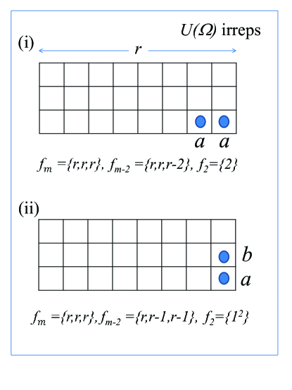
Figure 4: Young tableaux denoting the three-column $SU(\Omega)$ irreps $f_{m}=\{r,r,r\}$, $m=3r$ appropriate for BEGUE(2)-$SU(2)$. Removal of two boxes generating $m-2$ particle irreps $f_{m-2}$ are also shown in the figure. For (i) only the irrep $f_{2}=\{2\}$ will apply while for (ii) only $\{1^{2}\}$ will apply.

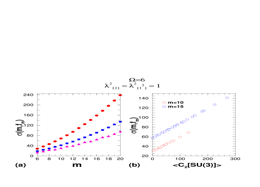
Figure 5: (a) Variation of spectral widths as a function of $m$ with fixed $f_{m}$. Shown are the results for $f_{m}$ as one-rowed $f_{m}^{(k)}$ irreps (red circles), two-rowed $f_{m}^{(k)}$ irreps (blue squares) and three-rowed $f_{m}^{(k)}$ irreps (magenta triangles). (b) Variation of spectral widths as a function of $f_{m}$ with fixed $m$. Shown are the results for $\Omega=6$ and $m=10,\;15$. Instead of showing $f_{m}$, we have used $\left\langle C_{2}[SU(3)]\right\rangle^{\tilde{f}_{m}}$.

V Embedded Gaussian Unitary Ensemble for spin one bosons: BEGUE(2)-SU(3) with $r=3$

Spin one boson systems, discussed in Ckmp-arx , possess $U(3\Omega)\supset U(\Omega)\otimes[SU(3)\supset SO(3)]$ symmetry. Instead of BEGOE(2) or BEGUE(2) generated by random two-body interactions preserving total spin $S$, it is also possible to consider interactions preserving the $SU(3)$ symmetry. Then, for the GUE version, we have BEGUE(2)-$SU(3)$ that corresponds to $r=3$ in Section 2. As $U(3)$ irreps will have, in young tableaux representation, maximum 3 rows, the $U(\Omega)$ irrep also will have maximum three rows. Given $m$ bosons in $\Omega$ number of sp levels, the allowed $U(\Omega)$ irreps are $\{f_{1},f_{2},f_{3},f_{4},\ldots,f_{\Omega}\}$ with $f_{1}+f_{2}+f_{3}=m$, $f_{1}\geq f_{2}\geq f_{3}\geq 0$ and $f_{i}=0$ for $i=4,5,\ldots,\Omega$. Because of the last condition we use simply $\{f_{1},f_{2},f_{3}\}$. For $f_{2}=0$ and $f_{3}=0$, we have totally symmetric irreps with $\{f_{1}\}=\{m\}$ and then all the results derived in Section 3 will apply directly. Similarly, for $f_{2}\neq 0$ and $f_{3}=0$, all the results of Section 4 will apply. Thus the non-trivial irreps for BEGUE(2)-$SU(3)$ are the $m$-boson irreps $f_{m}=\{f_{1},f_{2},f_{3}\}$ with $f_{3}\neq 0$. Given a $f_{m}$ in general there will be six $f_{m-2}$ and they are $\{f_{1}-2,f_{2},f_{3}\}$, $\{f_{1},f_{2}-2,f_{3}\}$, $\{f_{1},f_{2},f_{3}-2\}$, $\{f_{1}-1,f_{2}-1,f_{3}\}$, $\{f_{1}-1,f_{2},f_{3}-1\}$, $\{f_{1},f_{2}-1,f_{3}-1\}$. Therefore, as seen from Section 2, deriving analytical formulas for $P$’s, ${\cal Q}$’s and ${\cal R}$’s that determine $\left\langle H^{2}\right\rangle$, $\hat{\Sigma}_{11}$ and $\hat{\Sigma}_{22}$ will be cumbersome. One situation that is amenable to analytical treatment is for the irreps $\{r,r,r\}$, $m=3r$. For this class of irreps, the $f_{m-2}$ are simple as shown in Fig. 4. For $f_{m-2}=\{r,r,r-2\}$ we need $\Pi^{\prime}_{a}$ and $\Pi^{\prime\prime}_{a}$ and they are given by,

$$\Pi^{\prime}_{a}=\displaystyle\frac{3r}{\Omega+r-3}\;,\;\;\;\Pi^{\prime\prime}_{a}=\displaystyle\frac{6r(r-1)}{(\Omega+r-3)(\Omega+r-4)}\;.$$ (36)

Similarly, for $f_{m-2}=\{r,r-1,r-1\}$ we need $\tau_{ab}$, $\Pi^{(b)}_{a}$ and $\Pi^{(a)}_{b}$ and they are,

$$\tau_{ab}=-1\;,\;\;\;\Pi^{(b)}_{a}=\displaystyle\frac{3r}{2(\Omega+r-3)}\;,\;\;\;\Pi^{(a)}_{b}=\displaystyle\frac{2(r+1)}{(\Omega+r-2)}\;.$$ (37)

In addition, ratio of the $S_{\Omega}$ dimensions needed are,

$$\frac{{\cal N}_{r,r,r-2}}{{\cal N}_{r,r,r}}=\displaystyle\frac{2(r-1)}{(3r-1)}\;,\;\;\;\;\;\displaystyle\frac{{\cal N}_{r,r-1,r-1}}{{\cal N}_{r,r,r}}=\displaystyle\frac{r+1}{(3r-1)}\;.$$ (38)

With these, carrying out simplification of the formulas given in Table 1 will give the following results,

$$\begin{array}[]{l}P^{\{2\}}(m,\{r,r,r\})=-3r(r-1)\;,\;\;\;P^{\{1^{2}\}}(m,\{r,r,r\})=-\displaystyle\frac{3}{2}r(r+1)\;,\\ {\cal Q}^{\nu=0}(\{2\}:m,\{r,r,r\})=(3r)^{2}(r-1)^{2}\;,\\ {\cal Q}^{\nu=0}(\{1^{2}\}:m,\{r,r,r\})=\displaystyle\frac{(3r)^{2}(r+1)^{2}}{4}\;,\\ {\cal Q}^{\nu=1}(\{2\}:m,\{r,r,r\})=\displaystyle\frac{6(\Omega+1)(\Omega-3)r(r-1)^{2}(\Omega+r)}{(\Omega+2)}\;,\\ {\cal Q}^{\nu=1}(\{1^{2}\}:m,\{r,r,r\})=\displaystyle\frac{3(\Omega-1)(\Omega-3)r(r+1)^{2}(\Omega+r)}{2(\Omega-2)}\;,\\ {\cal Q}^{\nu=2}(\{2\}:m,\{r,r,r\})=\displaystyle\frac{3\Omega(\Omega-2)(\Omega-3)r(r-1)(\Omega+r)(\Omega+r+1)}{4(\Omega+2)}\;,\\ {\cal Q}^{\nu=2}(\{1^{2}\}:m,\{r,r,r\})=\displaystyle\frac{3\Omega(\Omega-3)(\Omega-4)r(r+1)(\Omega+r)(\Omega+r-1)}{8(\Omega-2)}\;,\\ {\cal R}^{\nu=0}(m,\{r,r,r\})=\displaystyle\frac{(3r)^{2}(r^{2}-1)}{2}\;,\\ {\cal R}^{\nu=1}(m,\{r,r,r\})=-\displaystyle\sqrt{\displaystyle\frac{\Omega^{2}-1}{\Omega^{2}-4}}\;3(\Omega-3)r(r^{2}-1)(\Omega+r)\;.\end{array}$$ (39)

Using these equations one can calculate the variances $\left\langle H^{2}\right\rangle$ and the covariances $\hat{\Sigma}_{11}$ and $\hat{\Sigma}_{22}$ for irreps of the type $\{r,r,r\}$. For example, Eq. (15) can be simplified using Eq. (39) to give a compact formula for spectral variances,

$$\begin{array}[]{rcl}\overline{\left\langle H^{2}\right\rangle^{m,\{r,r,r\}}}&=&\lambda^{2}_{\{2\}}\left[\displaystyle\frac{3}{2}r(r-1)(\Omega+r-3)(\Omega+r-4)\right]\\ \\ &+&\lambda^{2}_{\{1^{2}\}}\left[\displaystyle\frac{3}{4}r(r+1)(\Omega+r-2)(\Omega+r-3)\right]\;.\end{array}$$ (40)

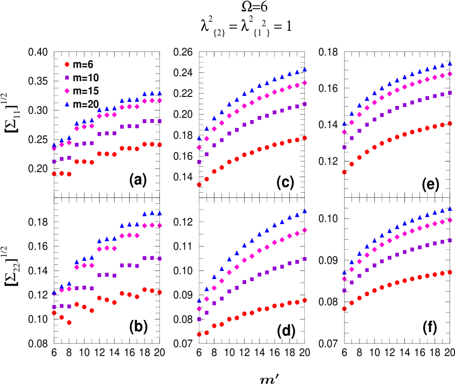
Figure 6: Self and cross correlations in energy centroids and spectral variances as a function of $m$ and $m^{\prime}$ for $\Omega=6$ (with fixed $f_{m}$ and $f_{m^{\prime}}$): (a) $[\Sigma_{11}(m,f_{m};m^{\prime},f_{m^{\prime}})]^{1/2}$ with $\{f_{m}\}=\{m/3,m/3,m/3\}$ for $m\mod 3=0$, $\{f_{m}\}=\{(m+2)/3,(m-1)/3,(m-1)/3\}$ for $m\mod 3=1$ and $\{f_{m}\}=\{(m+4)/3,(m-2)/3,(m-2)/3\}$ for $m\mod 3=2$ and similarly $f_{m^{\prime}}$ is defined; (b) $[\Sigma_{22}(m,f_{m};m^{\prime},f_{m^{\prime}})]^{1/2}$ with $\{f_{m}\}=\{m/3,m/3,m/3\}$ for $m\mod 3=0$, $\{f_{m}\}=\{(m+2)/3,(m-1)/3,(m-1)/3\}$ for $m\mod 3=1$ and $\{f_{m}\}=\{(m+4)/3,(m-2)/3,(m-2)/3\}$ for $m\mod 3=2$ and similarly $f_{m^{\prime}}$ is defined; (c) $[\Sigma_{11}(m,f_{m};m^{\prime},f_{m^{\prime}})]^{1/2}$ with $\{f_{m}\}=\{m/2,m/2\}$ for $m\mod 2=0$ and $\{f_{m}\}=\{(m+1)/2,(m-1)/2\}$ for $m\mod 2=1$ and similarly $f_{m^{\prime}}$ is defined; (d) $[\Sigma_{22}(m,f_{m};m^{\prime},f_{m^{\prime}})]^{1/2}$ with $\{f_{m}\}=\{m/2,m/2\}$ for $m\mod 2=0$ and $\{f_{m}\}=\{(m+1)/2,(m-1)/2\}$ for $m\mod 2=1$ and similarly $f_{m^{\prime}}$ is defined; (e) $[\Sigma_{11}(m,f_{m};m^{\prime},f_{m^{\prime}})]^{1/2}$ with $\{f_{m}\}=\{m\}$ and $\{f_{m^{\prime}}\}=\{m^{\prime}\}$; (f) $[\Sigma_{22}(m,f_{m};m^{\prime},f_{m^{\prime}})]^{1/2}$ with $\{f_{m}\}=\{m\}$ and $\{f_{m^{\prime}}\}=\{m^{\prime}\}$.

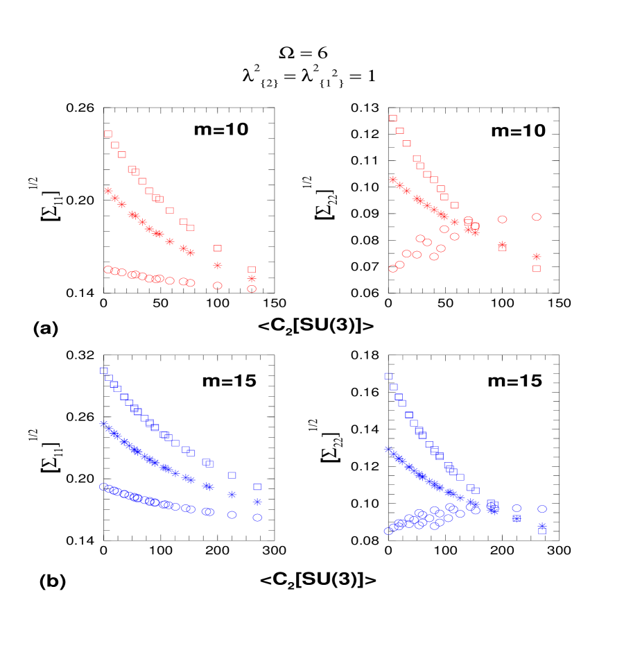
Figure 7: Self and cross correlations in energy centroids and spectral variances as a function of $f_{m}$ and $f_{m^{\prime}}$ for $\Omega=6$ (with fixed $m=m^{\prime}$). Results are shown for (a) $m=m^{\prime}=10$ with $f_{m}=\{10\}$ (red circles), $\{5,5\}$ (red stars) and $\{4,3,3\}$ (red squares) with all one, two and three rowed $f_{m^{\prime}}$ irreps; (b) $m=m^{\prime}=15$ with $f_{m}=\{15\}$ (blue circles), $\{8,7\}$ (blue stars) and $\{5,5,5\}$ (blue squares) with all one, two and three rowed $f_{m^{\prime}}$ irreps.

It is also possible to derive analytical results for the irreps $f_{m}=\{r+1,r,r\}$ and $\{r+2,r,r\}$ just as it was done for $\{4^{r},p\}$ irreps for EGUE(2)-$SU(4)$ ensemble in Ma-su4 . The results are as follows. For these irreps, the allowed $f_{m-2}$ irreps and the corresponding $\tau$ and $\Pi_{\ldots}$ functions are given in Table 2 and the dimension ratios in Table 3. Using these, for $f_{m}=\{r+1,r,r\}$ irreps, $P$, ${\cal Q}$ and ${\cal R}$ functions are,

$$\begin{array}[]{l}P^{\{2\}}(m,\{r+1,r,r\})=-r(3r-1)\;,\;\;\;P^{\{1^{2}\}}(m,\{r+1,r,r\})=-\displaystyle\frac{r}{2}(5+3r)\;,\\ {\cal Q}^{\nu=0}(\{2\}:m,\{r+1,r,r\})=r^{2}(3r-1)^{2}\;,\\ {\cal Q}^{\nu=0}(\{1^{2}\}:m,\{r+1,r,r\})=\displaystyle\frac{r^{2}}{4}(5+3r)^{2}\;,\\ {\cal Q}^{\nu=1}(\{2\}:m,\{r+1,r,r\})=\displaystyle\frac{r(1+\Omega)}{2+\Omega}\left[6r^{3}(-3+\Omega)+3(-3+\Omega)\Omega\right.\\ \left.+2r^{2}(-3+\Omega)(-2+3\Omega)+r\left\{-2+3(9-2\Omega)\Omega\right\}\right]\;,\\ {\cal Q}^{\nu=1}(\{1^{2}\}:m,\{r+1,r,r\})=\displaystyle\frac{r(-1+\Omega)}{2(-2+\Omega)}\left[-r(5+3r)^{2}\right.\\ \left.+\left\{-18+r(-18+r+3r^{2})\right\}\Omega+3(1+r)(2+r)\Omega^{2}\right]\;,\\ {\cal Q}^{\nu=2}(\{2\}:m,\{r+1,r,r\})=\displaystyle\frac{r(-3+\Omega)\Omega(1+r+\Omega)}{4(2+\Omega)}\left[8+3r^{2}(-2+\Omega)\right.\\ \left.-(-8+\Omega)\Omega+r(-2+\Omega)(1+3\Omega)\right]\;,\\ {\cal Q}^{\nu=2}(\{1^{2}\}:m,\{r+1,r,r\})=\displaystyle\frac{r(-3+\Omega)\Omega(-1+r+\Omega)}{8(-2+\Omega)}\left[-16+3r^{2}(-4+\Omega)\right.\\ \left.+r(-4+\Omega)(7+3\Omega)+\Omega(-14+5\Omega)\right]\;,\\ {\cal R}^{\nu=0}(m,\{r+1,r,r\})=\displaystyle\frac{r^{2}}{2}(-1+3r)(5+3r)\;,\\ {\cal R}^{\nu=1}(m,\{r+1,r,r\})=\displaystyle\frac{r}{24}\displaystyle\sqrt{\displaystyle\frac{\Omega^{2}-1}{\Omega^{2}-4}}\left[r^{3}(468-151\Omega)+153(-3+\Omega)\Omega\right.\\ \left.+r^{2}\left\{600+(283-151\Omega)\Omega\right\}-5r\left\{60+13\Omega(-7+2\Omega)\right\}\right]\;.\end{array}$$ (41)

Similarly, for $f_{m}=\{r+2,r,r\}$ irreps we have,

$$\begin{array}[]{l}P^{\{2\}}(m,\{r+2,r,r\})=-(3r^{2}+r+1)\;,\;\;\;P^{\{1^{2}\}}(m,\{r+2,r,r\})=-\displaystyle\frac{r}{2}(7+3r)\;,\\ {\cal Q}^{\nu=0}(\{2\}:m,\{r+2,r,r\})=(3r^{2}+r+1)^{2}\;,\\ {\cal Q}^{\nu=0}(\{1^{2}\}:m,\{r+2,r,r\})=\displaystyle\frac{r^{2}}{4}(7+3r)^{2}\;,\\ {\cal Q}^{\nu=1}(\{2\}:m,\{r+2,r,r\})=\displaystyle\frac{(1+\Omega)}{2(2+\Omega)}\left[-4(1+r+3r^{2})^{2}\right.\\ \left.+\left\{2+r\left\{3+r\left\{51+4r(-7+3r)\right\}\right\}\right\}\Omega+(2+11r+12r^{3})\Omega^{2}\right]\;,\\ {\cal Q}^{\nu=1}(\{1^{2}\}:m,\{r+2,r,r\})=\displaystyle\frac{r(-1+\Omega)}{2(-2+\Omega)}\left[-r(7+3r)^{2}\right.\\ \left.+(5+3r)(-6+r^{2})\Omega+\left\{10+3r(4+r)\right\}\Omega^{2}\right]\;,\\ {\cal Q}^{\nu=2}(\{2\}:m,\{r+2,r,r\})=\displaystyle\frac{\Omega}{4(2+\Omega)}\left[3r^{4}(-3+\Omega)(-2+\Omega)+(-1+\Omega)\Omega(2+\Omega)(3+\Omega)\right.\\ \left.+2r^{3}(-3+\Omega)(-2+\Omega)(4+3\Omega)+r^{2}(-3+\Omega)\Omega\left\{7+3\Omega(1+\Omega)\right\}\right.\\ \left.+r(-3+\Omega)\left\{22+\Omega\left\{42+\Omega(19+\Omega)\right\}\right\}\right]\;,\end{array}$$ (42)

$$\begin{array}[]{l}{\cal Q}^{\nu=2}(\{1^{2}\}:m,\{r+2,r,r\})=\displaystyle\frac{r(-3+\Omega)\Omega(-1+r+\Omega)}{8(-2+\Omega)}\left[-44+3r^{2}(-4+\Omega)\right.\\ \left.+r(-4+\Omega)(11+3\Omega)+\Omega(-12+7\Omega)\right]\;,\\ {\cal R}^{\nu=0}(m,\{r+2,r,r\})=\displaystyle\frac{r}{2}(7+3r)(1+r+3r^{2})\;,\\ {\cal R}^{\nu=1}(m,\{r+2,r,r\})=\displaystyle\frac{r}{48}\displaystyle\sqrt{\displaystyle\frac{\Omega^{2}-1}{\Omega^{2}-4}}\left[8(7+3r)(12+r+37r^{2})\right.\\ \left.+\left\{-1008+r\left\{1106+(241-289r)r\right\}\right\}\Omega+\left\{208-r(489+289r)\right\}\Omega^{2}\right]\;.\end{array}$$

Table 2: Formulas for the functions $\Pi_{--}^{(--)}$’s defined in Eq. (23) as required for $\{f_{m}\}$ irreps $\{r+1,r,r\}$ and $\{r+2,r,r\}$. Given also are the values of axial distances ($\tau_{--}$’s). Also, $\Pi_{a}^{(bc)}={r}/{(\Omega+r-3)}$ for both $\{f_{m}\}$ examples shown in the Table.

$\{f_{m}\}$	$\{f_{m-2}\}$	Required functions
$\{r+1,r,r\}$	$\{r+1,r,r-2\}$	$\Pi_{a}^{\prime}=\displaystyle\frac{8r}{3(\Omega+r-3)}$, $\Pi_{a}^{\prime\prime}=\displaystyle\frac{5r(r-1)}{(\Omega+r-3)(\Omega+r-4)}$
	$f(aa)$
	$\{r+1,r-1,r-1\}$	$\tau_{ab}=-1$, $\Pi_{a}^{(b)}=\displaystyle\frac{4r}{3(\Omega+r-3)}$, $\Pi_{b}^{(a)}=\displaystyle\frac{3(r+1)}{2(\Omega+r-2)}$
	$f(ab)$
	$\{r,r,r-1\}$	$\tau_{ac}=-3$, $\Pi_{a}^{(c)}=\displaystyle\frac{2r}{\Omega+r-3}$, $\Pi_{c}^{(a)}=\displaystyle\frac{r+3}{2(\Omega+r)}$
	$f(ac)$
$\{r+2,r,r\}$	$\{r+2,r,r-2\}$	$\Pi_{a}^{\prime}=\displaystyle\frac{5r}{2(\Omega+r-3)}$, $\Pi_{a}^{\prime\prime}=\displaystyle\frac{9r(r-1)}{2(\Omega+r-3)(\Omega+r-4)}$
	$f(aa)$
	$\{r+2,r-1,r-1\}$	$\tau_{ab}=-1$, $\Pi_{a}^{(b)}=\displaystyle\frac{5r}{4(\Omega+r-3)}$, $\Pi_{b}^{(a)}=\displaystyle\frac{4(r+1)}{3(\Omega+r-2)}$
	$f(ab)$
	$\{r+1,r,r-1\}$	$\tau_{ac}=-4$, $\Pi_{a}^{(c)}=\displaystyle\frac{2r}{\Omega+r-3}$, $\Pi_{c}^{(a)}=\displaystyle\frac{2(r+4)}{3(\Omega+r+1)}$
	$f(ac)$
	$\{r,r,r\}$	$\Pi_{c}^{\prime}=\displaystyle\frac{r+4}{2(\Omega+r+1)}$, $\Pi_{c}^{\prime\prime}=\displaystyle\frac{(r+3)(r+4)}{6(\Omega+r)(\Omega+r+1)}$
	$f(cc)$

Table 3: Dimension ratios with respect to the $S_{m}$ group for the examples in Table 2.

$\{f_{m}\}$	$\{f_{m-2}\}$	$\displaystyle\frac{{\cal N}_{\{f_{m-2}\}}}{{\cal N}_{\{f_{m}\}}}$
$\{r+1,r,r\}$	$\{r+1,r,r-2\}$	$\displaystyle\frac{5(r-1)}{3(3r+1)}$
	$\{r+1,r-1,r-1\}$	$\displaystyle\frac{2(r+1)}{3(3r+1)}$
	$\{r,r,r-1\}$	$\displaystyle\frac{(r+3)}{3(3r+1)}$
$\{r+2,r,r\}$	$\{r+2,r,r-2\}$	$\displaystyle\frac{9r(r-1)}{2(3r+2)(3r+1)}$
	$\{r+2,r-1,r-1\}$	$\displaystyle\frac{5r(r+1)}{3(3r+2)(3r+1)}$
	$\{r+1,r,r-1\}$	$\displaystyle\frac{4r(r+4)}{3(3r+2)(3r+1)}$
	$\{r,r,r\}$	$\displaystyle\frac{(r+3)(r+4)}{6(3r+2)(3r+1)}$

In addition to analytical results, as stated in Section 2, one can use the tables in Ma-su4 (also to a large extent Table 1) and obtain numerical results for the variation of spectral variances with the eigenvalues of the quadratic Casimir invariant of $U(\Omega)$ or equivalently $C_{2}[SU(3)]$, for various $(\Omega,m)$ values and also for both self and cross correlations in energy centroids and spectral variances. Note that For a $\Omega=6$ system with $\lambda_{\{2\}}^{2}=\lambda_{\{1^{2}\}}=1$ calculations are carried out for various choices of $m$ and $f_{m}$ and the results are shown in 5, 6 and 7. Let us mention that $C_{2}[SU(3)]$ for a irrep $\{f_{1},f_{2},f_{3}\}$ is given by the formula,

$$\left\langle C_{2}[SU(3)]\right\rangle^{\{f_{1},f_{2},f_{3}\}}=\lambda^{2}+\mu^{2}+\lambda\mu+3(\lambda+\mu)\;;\;\;\;\lambda=f_{1}-f_{2},\;\mu=f_{2}-f_{3}\;.$$ (43)

It is seen from Fig. 5a that the spectral widths will be largest for one rowed irreps and smallest for three row irreps for a fixed $m$. Also, widths as expected increase with $m$. Similarly, Fig. 5b shows that for a fixed $m$, widths increase as the eigenvalue of $C_{2}[SU(3)]$ increases and this is consistent with the observation in Fig. 5a as the eigenvalue of $C_{2}[SU(3)]$ is largest for totally symmetric irrep. Results in Fig. 6 show that: (i) the centroid and variance fluctuations increase with $m^{\prime}$ for fixed $m$ and vice-versa; (ii) they are larger for three rowed irreps compared to those for one rowed irreps; (iii) centroid fluctuations are much larger than variance fluctuations as seen before also for EGUE(2)-${\bf s}$ and EGUE(2)-$SU(4)$ ensembles. Similar trends are also seen for $m=m^{\prime}$ but varying $f_{m^{\prime}}$ with fixed $f_{m}$ and these results are shown in Fig. 7. A different trend is seen for the covariances in spectral variances for the totally symmetric irrep $f_{m}=\{m\}$ and $f_{m^{\prime}}$ varying. More importantly, the centroid and variance fluctuations are smallest for the ground state i.e., the most symmetric irrep for bosons. It is seen from Figs. 6 and 7 that the covariances in energy centroids are $\sim 15-25$% and the covariances in spectral variances are $\sim 8-15$%.

VI Conclusions

In this paper, given first is a general formulation for deriving lower order moments of the one- and two-point correlation functions in eigenvalues that is valid for any embedded random matrix for fermions as well as for bosons with $U(\Omega)\otimes SU(r)$ embedding and with two-body interactions preserving $SU(r)$ symmetry. Results of the present paper unify all the results known before for EGUE(2)’s and BEGUE(2)’s. Presented are new results for boson systems with $SU(r)$ symmetry, $r=2,3$. These results should be useful in future studies of two species boson systems and spin one boson systems. In future, it will be useful to derive analytical forms for $SU(\Omega)$ Racah coefficients Ko-07 ; Ma-su4 or develop tractable methods for their numerical evaluation to establish Gaussian form of the eigenvalue densities generated by embedded ensembles with $SU(r)$ symmetry both for boson and fermion systems.

References

(1) F.J. Dyson, A class of matrix ensembles, J. Math. Phys. 13, 90–97 (1972).
(2) V.K.B. Kota, SU(N) Wigner-Racah algebra for the matrix of
second moments of embedded Gaussian unitary ensemble of random matrices, J.
Math. Phys. 46, 033514/1-9 (2005).
(3) L. Benet, T. Rupp, and H.A. Weidenmüller, Spectral
properties of the -body embedded Gaussian ensembles of random matrices, Ann.
Phys. 292, 67–94 (2001).
(4) Z. Pluhar̆ and H.A. Weidenmüller, Symmetry Properties of
the -Body Embedded Unitary Gaussian Ensemble of Random Matrices, Ann. Phys.
(N.Y) 297, 344–362 (2002).
(5) T. Asaga, L. Benet, T. Rupp, and H.A. Weidenmüller,
Spectral properties of the -body embedded Gaussian ensembles of random
matrices for bosons, Ann. Phys. (N.Y.), 298, pp. 229–247 (2002).
(6) V.K.B. Kota,
Wigner-Racah algebra for embedded Gaussian unitary ensemble of random matrices
with spin, J. Math. Phys. 48, 053304/1-9 (2007).
(7) Manan Vyas and V.K.B. Kota, Spectral Properties of Embedded
Gaussian Unitary Ensemble of Random Matrices with Wigner’s Symmetry,
Ann. Phys. (N.Y.) 325, 2451–2485 (2010).
(8) Manan Vyas, N.D. Chavda, V.K.B. Kota and V. Potbhare, One plus
two-body random matrix ensembles for boson systems with -spin: Analysis using
spectral variances, J. Phys. A: Math. Theor. 45, 265203/1-33 (2012).
(9) H. N. Deota, N. D. Chavda, V. K. B. Kota, V. Potbhare and Manan
Vyas, Random matrix ensemble with random two-body interactions in
presence of a mean-field for spin one boson systems, in preparation.
(10) B.G. Wybourne, Symmetry Principles and Atomic Spectroscopy
(Wiley, New York, 1970).
(11) K.T. Hecht and J.P. Draayer, Spectral distributions and the
breaking of isospin and supermultiplet symmetries in nuclei, Nucl. Phys. A223, 285–319 (1974).
(12) K.T. Hecht, Summation relation for Racah coefficients, J.
Math. Phys. 15, 2148–2156 (1974).
(13) V.K.B. Kota, Two-body ensembles with group symmetries for chaos
and regular structures, Int. J. Mod. Phys. E 15, 1869–1883 (2006).
(14) T. Agasa, L. Benet, T. Rupp and H.A. Weidenmüller,
Non-ergodic behavior of the -body embedded Gaussian random ensembles for
bosons, Eur. Phys. Lett. 56, 340–346 (2001).
(15) N.D. Chavda, V. Potbhare and V.K.B. Kota, Statistical Properties
of Dense Interacting Boson Systems with One Plus Two-Body Random Matrix
Ensembles, Phys. Lett. A 311, 331–339 (2003).