The Rossiter-McLaughlin effect for exomoons or binary planets

Abstract

In this paper we study possible signatures of binary planets or exomoons on the Rossiter-McLaughlin (R-M) effect. Our analyses show that the R-M effect for a binary planet or exomoon during its complete transit phase can be divided into two parts. The first is the conventional one similar to the R-M effect from the transit of a single planet, of which the mass and the projected area are the combinations of the binary components; and the second is caused by the orbital rotation of the binary components, which may add a sine- or linear-mode deviation to the stellar radial velocity curve. We find that the latter effect can be up to several or several ten ${\rm m\,s^{-1}}$. By doing numerical simulations as well as analytical analyses, we illustrate that the distribution and dispersion of the latter effects obtained from multiple transit events can be used to constrain the dynamical configuration of the binary planet, such as, how the inner orbit of the binary planet is inclined to its orbit rotating around the central star. We find that the signatures caused by the orbital rotation of the binary components are more likely to be revealed if the two components of binary planet have different masses and mass densities, especially if the heavy one has a high mass density and the light one has a low density. Similar signature on the R-M effect may also be revealed in a hierarchical triple star system containing a dark compact binary and a tertiary star.

1 Introduction

Planets are not alone. For example, most of the planets in the Solar System have surrounding satellites or moons; not only some asteroids, but also many of the Kuiper Belt objects (e.g., Pluto and Charon) are in binaries; and recent observations have also revealed miscellaneous exoplanetary worlds, including multi-planetary systems (e.g., Kepler-11, HD 10180, Gliese 581; Lissauer et al. 2011; Lovis et al. 2010; Vogt et al. 2011; Forveille et al. 2011). Although the existence of exomoons or binary exoplanets have not been detected, various detection methods have been proposed, such as through transit light curves, transit timing and duration variations, direct imaging, microlensing, or Doppler spectroscopy of the host planet (e.g., Kipping et al. 2009; Simon et al. 2010, 2012; Sartoretti & Schneider 1999; and references therein). In this paper, we investigate possible observational signatures that a binary exoplanet system (if any) or an exoplanet plus one moon system would have on the Rossiter-McLaughlin (R-M) effect (McLaughlin, 1924; Rossiter, 1924) and how the orbital configurations of the system could be revealed through the signatures. For simplicity, below we also call the one exoplanet plus one moon system as a binary planet, although the two components have very different masses. Existence of binary planets and statistics on their dynamical configurations should shed new light on the formation and evolution of planetary systems and the search for a habitable world.

When a planet transits in front of a rotating star, it blocks part of the light emitted from the stellar surface, and the blocked region shifts with the transiting of the planet. As different parts of the stellar surface may have different line-of-sight velocities to the observer, the shifting of the blocked region results in either blueshift or redshift of observed stellar spectral lines and further the deviation of the inferred radial velocity of the stellar motion (i.e., the R-M effect). The deviation of the stellar radial velocity provides a way to measure the misalignment between the stellar spin and the planetary orbital angular momentum, and recent measurements of the R-M effects have found that some exoplanets are on highly inclined orbits relative to the spin of the star (e.g., retrograde or polar orbits; Winn et al. 2009; Collier Cameron et al. 2010). For the similar reasons, if the transiting planet is a binary, the binary with different physical properties and orbital configurations (e.g., radii, inclination) may block the stellar surface in different ways, and hence the shift of stellar spectral lines and the deviation of its radial velocity curve may have different signatures from those expected from the transit of one single planet. The gravitation from a binary planet is also different from that from one single planet with the same total mass, but the resulted deviation in the dynamical motion of the star is generally small within each transit duration (see justification in Section 3.3 below). In this paper, we isolate and illustrate the effects on the observed stellar radial velocity due to the different light blocking ways.

Most of the modeling of the R-M effect for planetary systems were developed for a single planet rotating around a star. The R-M effect for exomoon systems was numerically modeled by Simon et al. (2010), where the exomoon has a much smaller mass and radius than its host planet and the moon effects are modeled as a small perturbation added to the effect caused by a single planet. Their modeling includes the fitting to the numerous dynamical parameters of the systems, including instantaneously and fast evolving ones. In this paper we present a comprehensive analysis and investigation on the R-M effect for a binary planet system, where the satellite mass is not limited to be small but can be comparable to the host planet mass. We include the effects from the dynamical evolution of the binary planet system during multiple transits and their different dynamical configurations. Our detailed treatments average out the effects from some instantaneously changing dynamical angles and include the evolutionary patterns of those relatively fast changing ones, so that we can focus on the effects from different inner orbital inclinations of the binary planet relative to its orbit rotating around the central star.

The paper is organized as follows. In Section 2, we describe the geometric configuration of the system to be studied in this paper (i.e., a binary planet transiting in front of a star) and related dynamical approximations. In Section 3, we investigate how the R-M effect is affected by a binary planet and how the different orbital configurations could be inferred from the deviation of the stellar radial velocity curves, together with the transit of the stellar light curves. We explore the parameter space of binary planets that are likely to be revealed in observations. We also extend the results to hierarchical triple star systems in which a binary star (e.g., a compact stellar remnant plus a brown dwarf or planet) is transiting in front of a tertiary star gravitationally bound to the system. Section 4 contains a summary and a discussion.

2 Geometric configuration and dynamical description of the system

Consider that a binary planet is rotating around a star (see Fig. 1). For convenience, we shall call the binary planet as the “inner” binary, and call the star and the center of the mass of the binary planet as the “outer” binary. We denote the mass and the radius of the star as $m_{*}$ and $R_{*}$. The projected area of the star onto the sky is $A_{*}=\pi R_{*}^{2}$, and it has a surface brightness of $I_{*}$. The angular velocity of the stellar spin is $\Omega_{*}$. We denote the component masses of the inner binary as $m_{1}$ and $m_{2}$ ($m_{1}\geq m_{2}$), and the component radii as $R_{1}$ and $R_{2}$, respectively. Here we have $m_{1}+m_{2}\ll m_{*}$. The projected areas of the two components onto the sky are $A_{1}=\pi R_{1}^{2}$ and $A_{2}=\pi R_{2}^{2}$, respectively (see the parameter list in Table 1).

Table 1: List of parameters.

Object	Property	Symbol
Central star	mass	$m_{*}$
	radius	$R_{*}$
	sky-projected area	$A_{*}$
	surface brightness	$I_{*}$
	unit vector of spin	$\vec{n}_{*}$
	inclination of spin	$i_{*}$
	spin angular velocity	$\Omega_{*}$
Binary planet	mass	$m_{1},m_{2}$
	radius	$R_{1},R_{2}$
	sky-projected area	$A_{1},A_{2}$
	mass density	$\rho_{1},\rho_{2}$
Orbit of outer binary	semimajor axis	$a$
	eccentricity	$e$
	unit vector of angular momentum	$\vec{n}$
	angular velocity	$\omega$
	sky-projected angle between $\vec{n}$ and $\vec{n}_{*}$	$\lambda$
	inclination to the line of sight	$i$
Orbit of inner binary	semimajor axis	$d$
	distance to center of mass	$d_{1},d_{2}$
	eccentricity	$e^{\prime}$
	unit vector of angular momentum	$\vec{n}^{\prime}$
	angular velocity	$\omega^{\prime}$
	sky-projected angle between $\vec{n}^{\prime}$ and $\vec{n}_{*}$	$\lambda^{\prime}$
	inclination to the line of sight	$i^{\prime}$
Precession of $\vec{n}^{\prime}$ around $\vec{n}$	angle between $\vec{n}$ and $\vec{n}^{\prime}$	$\theta$
	angular velocity	$\Omega$

Note. — See details in Section 2 and Fig. 1.

We describe the dynamical motion of the system through the two components: (i) the orbital motion of the outer binary, and (ii) the orbital motion of the inner binary. The orbital motion of the inner binary includes the precession of its orbital angular momentum around the orbital angular momentum of the outer binary, as described below.

The orbital configuration of the system is indicated in a reference frame as shown in Figure 1. In Figure 1, the center of the star is located at the origin $O$. The $y$-axis is directed toward the observer, and the $z$-axis is chosen so that the stellar spin axis lies on the $y$-$z$ plane. The inclination angle of the stellar spin relative to the $y$-axis is denoted by $i_{*}$ ($0\leq i_{*}\leq\pi$). The unit vector of the orbital angular momentum of the outer binary is denoted by $\vec{n}$, and we define $\lambda$ by the angle between the $z$-axis and the projected vector of $\vec{n}$ onto the $x$-$z$ plane ($0\leq\lambda<2\pi$). The orbital inclination angle to the observer $i$ is defined by the angle between $\vec{n}$ and the $y$-axis. Thus, we have $\vec{n}=(\sin\lambda\sin i,\cos i,\cos\lambda\sin i)$. The outer binary has a semimajor axis of $a$ and an angular velocity $\omega=[G(m_{*}+m_{1}+m_{2})/a^{3}]^{1/2}$. For simplicity, the eccentricity of the outer binary $e$ is assumed to be zero, unless otherwise specified.

Similarly, we denote the unit vector of the orbital angular momentum of the inner binary by $\vec{n}^{\prime}$, and we define $\lambda^{\prime}$ by the angle between the $z$-axis and the projected vector of $\vec{n}^{\prime}$ onto the $x$-$z$ plane, and define the orbital inclination angle $i^{\prime}$ to the observer by the angle between $\vec{n}^{\prime}$ and the $y$-axis. We have $\vec{n}^{\prime}=(\sin\lambda^{\prime}\sin i^{\prime},\cos i^{\prime},\cos\lambda^{\prime}\sin i^{\prime})$. The angle between $\vec{n}$ and $\vec{n}^{\prime}$ is denoted by

$$\theta\equiv\arccos(\vec{n}\cdot\vec{n}^{\prime}),\quad 0\leq\theta\leq\pi.$$ (1)

The semimajor axis and angular velocity of the inner binary are denoted by $d$ and $\omega^{\prime}=[G(m_{1}+m_{2})/d^{3}]^{1/2}$, respectively. The eccentricity of the inner binary $e^{\prime}$ is assumed to be zero, unless specially discussed in some cases below. Note that the semimajor axis of the inner binary is limited by the Hill radius $d_{H}$ and the Roche limit $d_{R}$, i.e.,

$$d\lesssim d_{H}\equiv a\left(\frac{m_{1}+m_{2}}{3m_{*}}\right)^{1/3}\simeq 0.07{\rm AU}\left(\frac{a}{1{\rm AU}}\right)\left(\frac{m_{1}+m_{2}}{M_{J}}\right)^{1/3}\left(\frac{{M_{\odot}}}{m_{*}}\right)^{1/3}$$ (2)

$$d\gtrsim d_{R}\equiv R_{1}\left(2\frac{\rho_{1}}{\rho_{2}}\right)^{1/3},$$ (3)

where $M_{\odot}$ is the solar mass, $M_{J}$ is the Jupiter mass, $\rho_{i}$ ($=\frac{3m_{i}}{4\pi R_{i}^{3}}$, $i=1,2$) is the mass density of each component of the inner binary. An inner binary with a larger semimajor axis will be tidally broken up by the gravitation from the star.

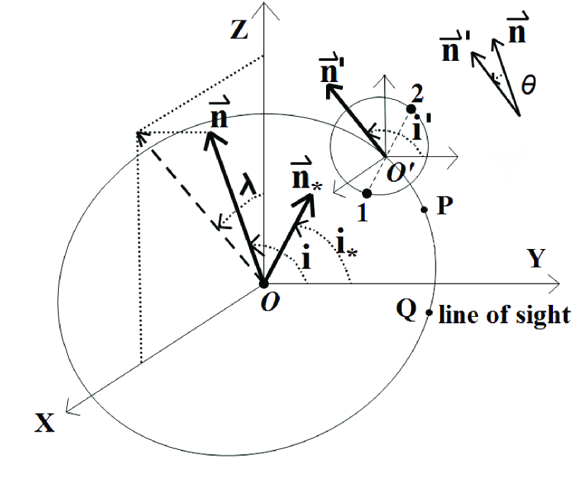
Figure 1: Schematic diagram for the orbital configuration of the system in which a binary planet is rotating around a star. The star is located at the origin $O$. The two components of the binary planet are denoted by “1” and “2”, and their center of mass is labeled by $O^{\prime}$. For brevity, the star and the binary planet are all indicated by points, without illustrating their physical radii in the figure. The observer is along the direction of the $y$-axis. The spin direction of the star $\vec{n}_{*}$ is located at the $y$-$z$ plane. The round curve centering at $O$ represents the orbit of the center of mass of the binary planet rotating around the star. The $\vec{n}$ represents the unit vector of the orbital angular momentum of the outer binary, and the $\vec{n}^{\prime}$ represents the unit vector of the orbital angular momentum of the inner binary (binary planet). The angle between $\vec{n}$ and $\vec{n}^{\prime}$ is defined by $\theta$ in Table 1. Point $P$ is the pericenter of the orbital plane of the outer binary if the orbit is eccentric, and point $Q$ is located on the intersection line of that orbital plane and the plane where both the vector $\vec{n}$ and the $y$-axis are located. The angle between $\overrightarrow{OP}$ and $\overrightarrow{OQ}$ ($\angle POQ$ not labeled in the figure for visual clarity) is used in equation (18) later. For other labeled angles, see also Table 1 and Section 2.

In general, the orbital parameters of the outer binary and the inner binary may evolve with time under the three-body interactions of the star and the binary planet. But under some conditions, their dynamical motion can be much simplified as follows.

• The orbital parameters of the outer binary ($a$, $e$, $\vec{n}$, $i$, $\lambda$) can be approximately constant, if the semimajor axis of the inner binary is much smaller than the Hill radius $d_{H}$.

• The semimajor-axis of the inner binary $d$ can also be approximately constant if it is much smaller than the Hill radius. Both the inclination $i^{\prime}$ and the projected angle $\lambda^{\prime}$ of the inner binary may change with time due to the evolution of $\vec{n}^{\prime}$. The evolution of $\vec{n}^{\prime}$ depends on the angle $\theta$ between the orbital angular momenta of the inner and the outer binaries (i.e., $\vec{n}^{\prime}$ and $\vec{n}$; e.g., Ford et al. 2000).

  1. If the angle $\theta$ or $180\arcdeg-\theta$ is small (e.g., $\lesssim 40\arcdeg$, the Kozai angle; Kozai 1962), the $\vec{n}^{\prime}$ precesses around $\vec{n}$ approximately at a constant angular velocity $\Omega\sim\omega^{2}\cos\theta/\omega^{\prime}$, and the angle $\theta$ can also be approximately constant. The angles $i^{\prime}$ and $\lambda^{\prime}$ change periodically with the precession of $\vec{n}^{\prime}$. As one transit duration $\delta t$ ($\sim\omega^{-1}R_{*}/a$) is generally much shorter than the precession timescale of $\vec{n}^{\prime}$, the $\vec{n}^{\prime}$ (and $i^{\prime}$, $\lambda^{\prime}$) can be approximated as constant during each transit duration.

  2. If the angle $\theta$ is about in the range from $40\arcdeg$ to $140\arcdeg$, the Kozai mechanism affects the evolution of the orbital parameters of the inner binary, in which the angle $\theta$ and the eccentricity $e^{\prime}$ exchange at a period $\sim 2\pi\omega^{\prime}/\omega^{2}$ due to angular momentum transfer and the conservation of the quantity $C_{K}\equiv\sqrt{1-e^{\prime 2}}\cos\theta$ (see an example shown in Fig. 4 below). During the oscillation, the eccentricity of the inner binary can be induced to high values close to 1, and thus the inner binary is likely to be destroyed by collision of its two components. If there exist other moons in the system, one component of the binary is also likely to be ejected from the system or collide with one of the moons. The Jovian system is such an example influenced by the Kozai mechanism, and almost all the inclinations of their moons are out of the angle range. Here we ignore other effects from the planet (e.g., tides, the general relativistic effect), which would limit the influence of the Kozai mechanism. The limitation would become relatively significant for a system with small $d$ but large $a$. For example, Uranus is farther from the sun and its inner moons (with $R_{*}/a\simeq 2.4\times 10^{-4}$ and $a/d\sim 5\times 10^{3}-6\times 10^{4}$) are on polar orbits relative to its orbital plane surrounding the sun (e.g., Murray & Dermott 1999).

  Below we do not focus on case (b).

3 Transit of a binary planet and its signatures on the R-M effect

3.1 Transit light curves

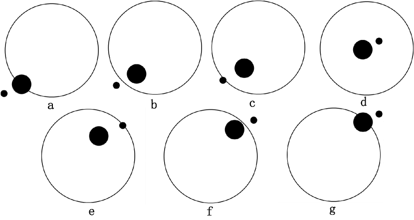
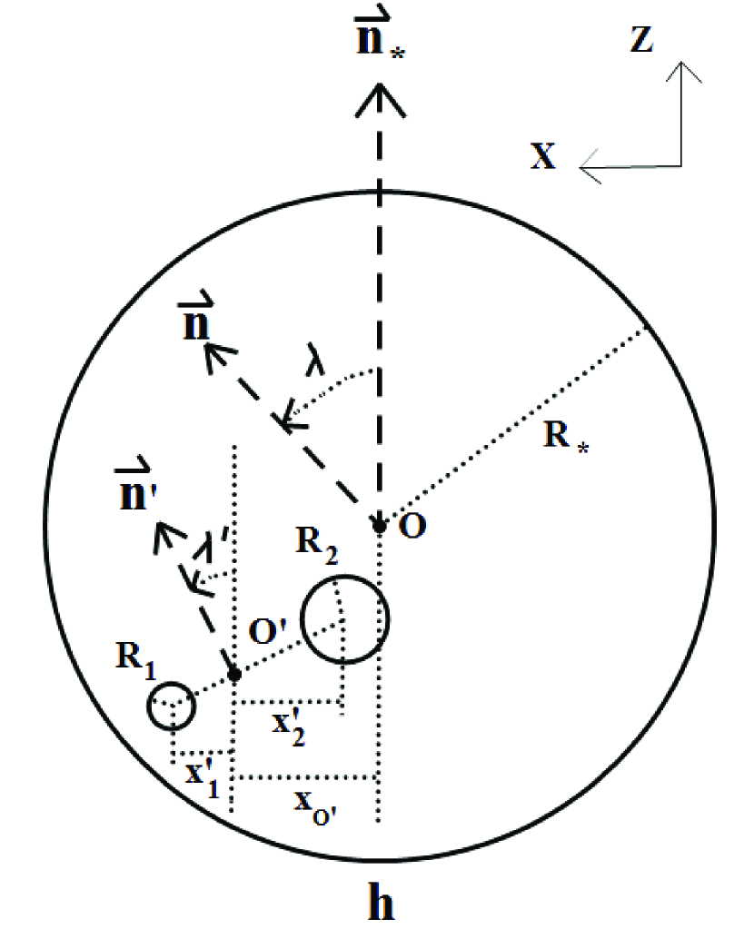
Figure 2: Panels (a)–(g): schematic diagram for transit of a binary planet (small shaded circles) in front of a star (big open circle). The observer is located in the direction of pointing out of the paper surface. The binary planet is transiting from left to right. Panels (a)–(c): ingress phase; panel (d): complete transit phase of the binary planet; panels (e)–(g): egress phase. In this example, the rotation of the binary planet is fast enough so that the small component has changed its relative position from the left side to the right side of the big one during the complete transit phase (d). See details in Section 3.1. Panel (h): schematic diagram for the geometry of the system during the complete transit phase of a binary planet. The sizes of the star and the binary planet are all illustrated in the panel. The dashed lines represent the projection of the labeled vectors onto the sky. See also Table 1 for the meaning of labeled parameters.

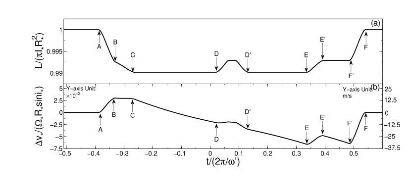
Figure 3: Example of transit light curve and stellar radial velocity anomaly for transit of a binary planet in front of a star. The reflected light from the surface of the binary planet is ignored for simplicity. Panel (a): normalized observational stellar light curve $L(t)/(\pi I_{*}R_{*}^{2})$. Panel (b): observational radial velocity anomaly of the star. The left y-axis in panel (b) represents the dimensionless velocity values, and the right y-axis represents the physical values of the $\Delta v_{*}$ by assuming $\Omega_{*}R_{*}\sin i_{*}=5{\rm km\,s^{-1}}$ (similarly for $\Delta v_{b}$ in Fig. 5 and $\Delta v_{*}$ in Fig. 9. Related parameters used for this example are as follows: $\log(\frac{m_{1}+m_{2}}{m_{*}})=-2$, $\rho_{1}/\rho_{2}=5$, $m_{1}/m_{2}=1.2$, $a/d=125$, $R_{*}/a=0.02$, $\frac{A_{1}+A_{2}}{A_{*}}=0.01$, $\lambda=35\arcdeg$, $i=89.5\arcdeg$, and $\theta=10\arcdeg$. See details in Section 3.2.

When a binary planet transits in front of a star (see a schematic diagram in Fig. 2), the stellar light curves may be imprinted with signatures of the binary planet. We illustrate one example of the normalized transit light curve in Figure 3 (see panel a). The observational transit curve is obtained by $L\equiv\int\int I(x,z)dxdz$, where $I(x,z)$ is the observational stellar surface brightness at position $(x,z)$. During the transit, part of the stellar surface is blocked by the planets, and we set

$$I(x,z)=\cases{I_{*},&unblocked region with $x^{2}+z^{2}\leq R_{*}^{2}$,\cr 0,&otherwise,}$$ (4)

For simplicity, the limb-darkening effect of the stellar surface brightness is ignored in this paper. We use a full three-body simulation to obtain the dynamical motion of the system. The dynamical motion of the binary planet relative to the star determines the shifting of the blocked region during the transit. The following phases during the transit are illustrated in Figures 2 and 3.

• Ingress phase: at the beginning of the transit, at least one component of the binary planet starts to block the stellar light, but the projected areas of the two components have not been fully enclosed by the projected stellar surface (e.g., the “AC” part in Fig. 3).

• Complete transit phase of the binary planet: both the projected areas of the two components have been fully enclosed by the projected stellar surface (e.g., the “CE” part in Fig. 3). Generally the two planets are more likely to spend most of the transit time in that phase when $i$ is close to $\pi/2$. The $d<2R_{*}$ can be roughly taken as a condition for the occurrence of this phase during the transit. If the binary planet has a sufficiently large $\omega^{\prime}$, it is likely that during the transit, their orbital evolution leads to the evolution of their projected areas from non-overlap to overlap, and to non-overlap again, for which a “bulge” (the “DD^′” part in Fig. 3) are shown in the light curve.

• Egress phase: at least one component of the binary planet has transited to the other end of the projected stellar surface and its projected area is not fully enclosed by the projected stellar surface again (e.g., the “EF” part in Fig. 3). The “E^′F^′” flat part of the light curve in Fig. 3a represents the period in which one component has fully moved out of the projected stellar surface, but the other one is still completely inside.

The transit of a binary is different from that of a single body. As illustrated above, the binary may enter or exit the transit one by one, or the projected areas of the two components may overlap, so that some special features can be shown in the transit light curve (e.g., some step changes or “bulges”). Some properties of the binary planet (e.g., radii of its two components, and its angular velocity and semimajor axis if its $\omega^{\prime}$ is sufficiently fast; Sato & Asada 2009) can be extracted from the features. In addition, the transit duration variation and the transit timing variation measured from the light curves have also been proposed to obtain the exomoon mass and the semimajor axis of the moon’s orbit (Kipping, 2009a, b). Below we illustrate that the orbital configuration of the binary planet can be further constrained by the evolution curve of the observational stellar radial velocity.

Note that the velocity in Figure 3 (similarly in Fig. 5 below) is expressed in a dimensionless quantity, where the stellar parameters involved in the normalization could be non-trivial to estimate in realistic systems and would be done through other independent methods and abundant knowledge in stellar astrophysics.

3.2 Stellar radial velocity anomaly and orbital configuration of a binary planet

As mentioned in the Introduction, a binary planet may leave signature on the observational radial velocity of the star, as well as on its light curve. The apparent stellar radial velocity anomaly due to the blocking of the stellar light is given by

$$\Delta v_{*}=-K\frac{\int\int xI(x,z)dxdz}{\int\int I(x,z)dxdz}$$ (5)

(e.g., Ohta, Taruya, & Suto 2005; Winn et al. 2005), where $K\equiv\Omega_{*}\sin i_{*}$ is the line-of-sight component of the spin angular velocity and may be observationally constrained from the stellar spectrum. Applying equation (5) to the example shown in Figure 3a, we obtain the evolution curve of its corresponding radial velocity anomaly in Figure 3b (see also Fig. 1 in Simon et al. 2009).

Below we demonstrate how the dynamical configuration of the binary planet is incorporated into the evolution curve of the stellar radial velocity anomaly. For simplicity, we consider the complete transit phase of the binary planet. And we analyze the case in which the projected areas of the two planets do not overlap, and the non-overlap is likely to be true during most of the transit time especially if $R_{1}+R_{2}\ll d$ or $|\pi/2-i^{\prime}|\gtrsim(R_{1}+R_{2})/d$. Thus, the stellar radial velocity anomaly can be simplified as follows:

$$\Delta v_{*}=K\frac{x_{1}A_{1}+x_{2}A_{2}}{A_{*}-A_{1}-A_{2}},$$ (6)

where $x_{1}=x_{O^{\prime}}+x_{1}^{\prime}$ and $x_{2}=x_{O^{\prime}}+x_{2}^{\prime}$ are the $x$-coordinates of the center of each planet, respectively (see Fig. 2h),

$$x_{O^{\prime}}=a(1-\sin^{2}\lambda\sin^{2}i)^{1/2}\sin[\omega(t-t_{0})]\quad(\mbox{if }e=0)$$ (7)

is the $x$-coordinate of the center of mass of the binary planet, $t_{0}$ is set so that $x_{O^{\prime}}=0$ at $t=t_{0}$,

$$x_{1}^{\prime}=d_{1}(1-\sin^{2}\lambda^{\prime}\sin^{2}i^{\prime})^{1/2}\sin[\omega^{\prime}(t-t_{0})+\phi]$$ (8)

and

$$x_{2}^{\prime}=-d_{2}(1-\sin^{2}\lambda^{\prime}\sin^{2}i^{\prime})^{1/2}\sin[\omega^{\prime}(t-t_{0})+\phi]$$ (9)

are the $x$-coordinates of the two planets relative to their center of mass, $d_{1}$ and $d_{2}$ are the distances of the two planets to their center of mass, and $\phi$ represents the orbital phase of the inner binary. The $y$-coordinates of the planets along the line of sight do not appear explicitly in equation (6), but they are involved in the expression through the angles $\omega^{\prime}(t-t_{0})$ and $\phi$. Applying equations (7)–(9) to equation (6), we have

$$\Delta v_{*}=\Delta v_{O^{\prime}}+\Delta v_{b},$$ (10)

where

$$\Delta v_{O^{\prime}} = K\frac{a(A_{1}+A_{2})}{A_{*}-A_{1}-A_{2}}(1-\sin^{2}\lambda\sin^{2}i)^{1/2}\sin[\omega(t-t_{0})],$$ (11)

$$\Delta v_{b} = K\frac{d_{1}A_{1}-d_{2}A_{2}}{A_{*}-A_{1}-A_{2}}(1-\sin^{2}\lambda^{\prime}\sin^{2}i^{\prime})^{1/2}\sin[\omega^{\prime}(t-t_{0})+\phi].$$ (12)

The $\Delta v_{*}$ is composed of the two terms, $\Delta v_{O^{\prime}}$ and $\Delta v_{b}$.

• The $\Delta v_{O^{\prime}}$ gives the radial velocity anomaly as if the transiting body is a single body with the values of its mass and projecting area being the total ones of the binary and contains the orbital configuration of the outer binary, i.e., the angles $\lambda$ and $i$. This R-M effect due to the transit of a single planet has been used to extract those angles of some realistic exoplanetary systems. Together with some assumption or observational evidence on the possible distribution of the inclination of the stellar spin $i_{*}$, the orbital inclination of the planet relative to the stellar spin (i.e., the angle between $\vec{n}$ and $\vec{n}_{*}$) can be further statistically constrained (e.g., Winn et al. 2009). This inclination has also been measured in a number of realistic systems through the photometric anomalies exhibited in transit light curves, which are interpreted as passages of the planet over dark starspots (e.g., Sanchis-Ojeda & Winn 2011).

• The $\Delta v_{b}$ comes from the relative motion of the inner binary, for which the sine mode of equation (12) represents its periodical orbital motion. The information on the orbital configuration of the inner binary ($\lambda^{\prime}$, $i^{\prime}$) comes from $\Delta v_{b}$, and we focus on the effects of this term in this paper.

Within one transit duration, as $\omega\delta t\sim R_{*}/a\ll 1$, the $\Delta v_{O^{\prime}}$ in equation (11) can be simplified to be linear with time as follows,

$$\Delta v_{O^{\prime}}=K\frac{a(A_{1}+A_{2})}{A_{*}-A_{1}-A_{2}}(1-\sin^{2}\lambda\sin^{2}i)^{1/2}\omega(t-t_{0}).$$ (13)

If the sine mode in $\Delta v_{b}$ can be identified in the observations, its period and amplitude can be used to constrain the value of $\omega^{\prime}$ and the geometric configuration ($\lambda^{\prime}$, $i^{\prime}$). If $\omega^{\prime}\delta t\sim\frac{\omega^{\prime}}{\omega}\frac{R_{*}}{a}\ll 1$, the $\Delta v_{b}$ in equation (12) can be reduced to be also linear with time as follows

$$\Delta v_{b} = K\frac{d_{1}A_{1}-d_{2}A_{2}}{A_{*}-A_{1}-A_{2}}(1-\sin^{2}\lambda^{\prime}\sin^{2}i^{\prime})^{1/2}[\sin\phi+\omega^{\prime}(t-t_{0})\cos\phi],$$ (14)

and the slope of the $\Delta v_{*}$–$t$ curve during the complete transit phase is given by

$$k\equiv\frac{d\Delta v_{*}}{dt}=k_{O^{\prime}}+k_{b}\cos\phi,$$ (15)

where

$$k_{O^{\prime}}=K\frac{a(A_{1}+A_{2})}{A_{*}-A_{1}-A_{2}}(1-\sin^{2}\lambda\sin^{2}i)^{1/2}\omega$$ (16)

and

$$k_{b}=K\left(\frac{d_{1}A_{1}-d_{2}A_{2}}{A_{*}-A_{1}-A_{2}}\right)(1-\sin^{2}\lambda^{\prime}\sin^{2}i^{\prime})^{1/2}\omega^{\prime}.$$ (17)

The $k_{O^{\prime}}$ is constant with time as $\lambda$ and $i$. The $k_{b}$ depends on the orbital configuration of the inner binary ($\lambda^{\prime}$, $i^{\prime}$), which is usually constant within one transit duration, as mentioned in Section 2.

Even if the eccentricity of the outer binary $e$ is non-zero, but has a low or moderate value [e.g. $e$=0.3, so that the linear approximation of $\omega(t-t_{0})$ in eq. 13 is still valid], the expressions for $\Delta v_{O^{\prime}}$ and $k_{O^{\prime}}$ can be modified simply by replacing $a$ with $ga$ in equations (13) and (16), where the factor

$$g=(1-e^{2})^{-1/2}[1+e\cos(\alpha+\angle POQ)],$$ (18)

the angle $\alpha$ is defined by $\tan\alpha=\sin\lambda\cos i/\cos\lambda$ and $\cos\alpha=-\cos\lambda/(1-\sin^{2}\lambda\sin^{2}i)^{1/2}$, and the meaning of the angle $\angle POQ$ is indicated in Figure 1.

In a longer time period $\Delta t$($>\delta t$), the evolution of $\lambda^{\prime}$ and $i^{\prime}$ is determined by the precession of $\vec{n}$ around $\vec{n}^{\prime}$ and the value of the angle $\theta$. In this case, we discuss the linear mode in the following two regimes.

• If $\Omega\Delta t\ll 1$ (i.e., $\Delta t$ is much shorter than the precession timescale, but covers multiple transit events), $k_{b}$ is still roughly constant. The distribution of the phases $\phi/2\pi$ follows the distribution of $n\omega^{\prime}/\omega$ ($n$: integer). In general, unless $\omega^{\prime}/\omega$ is an integer, $\phi$ is uniformly distributed between 0 and $2\pi$, and we can get the average of the slopes over the multiple transits as follows

  $$\overline{k}=k_{O^{\prime}},$$ (19)

  which can be used to constrain the sky-projected angle $\lambda$. The rms of the slopes is

  $$\left[\overline{(k-\overline{k})^{2}}\right]^{1/2}=\frac{1}{2}k_{b}.$$ (20)

  The value of $\theta$ is a function of $\lambda^{\prime}$ and $i^{\prime}$ (see eq. 1), and equation (20) can be used as an observational constraint for statistical determination of the probability distribution of $\theta$.

• If $\Omega\Delta t\gtrsim 1$, $k_{b}$ changes due to the precession of $\vec{n}$ and the variation of $\lambda^{\prime}$ and $i^{\prime}$. Here we only discuss the case with $0\lesssim\theta\lesssim 40\arcdeg$ or $140\arcdeg\lesssim\theta\lesssim 180\arcdeg$. As seen from Figure 4, the evolution pattern of $f\equiv(1-\sin^{2}\lambda^{\prime}\sin^{2}i^{\prime})^{1/2}$ is different with different $\theta$. Note that the evolution pattern for $\pi-\theta$ ($0\lesssim\theta\lesssim 40\arcdeg$) can be obtained by reversing the time in the pattern for $\theta$, as the precession direction for $\theta>90\arcdeg$ is along $-\vec{n}$. The slope of $k$ should distribute within the envelope of $f$, and the magnitude of the variation of $f$ increases with increasing $\theta$ (for $\theta<90\arcdeg$). Hence the distribution of the slopes can be used to constrain the value of $\theta$ (or $|90\arcdeg-\theta|$). We illustrate such an example in Figure 5(c)–(e), by doing full three-body numerical simulations on dynamical evolution of a binary planet rotating around a star and obtaining its multiple transiting events.

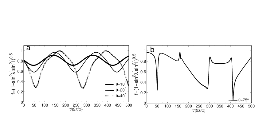
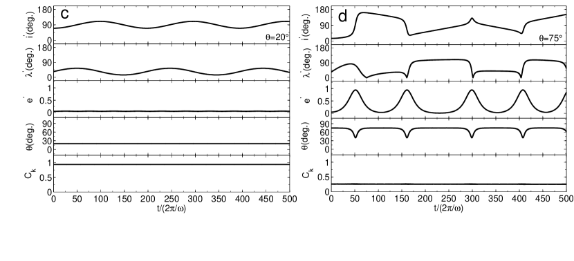
Figure 4: Examples of the orbital evolution of a binary planet rotating around a star, calculated from a full three-body numerical simulation. The related parameters used are the same as those in Fig. 3 except the value of $\theta$. The variable of $f(\theta,t)$ affects the amplitude or slope of the stellar radial velocity anomaly curve (see eqs. 12 and 17). Panel (a) is mainly for $\theta\lesssim 40\arcdeg$; and panel (b) gives an example with $\theta=75\arcdeg$, where the Kozai mechanism is effective. In panel (a), different curves of $f$ represent the evolution under different $\theta$, which produces different slope distributions of the stellar radial velocity anomaly curves, given multiple transit observations. Panels (c) and (d) show the evolution of some other parameters corresponding to the cases shown in panel (a) and (b), respectively. In panel (b) ($\theta=20\arcdeg$), the parameters $e^{\prime}$, $\theta$, and $C_{K}$ are almost constant with time, and the angles $\lambda^{\prime}$ and $i^{\prime}$ evolve periodically due to the precession of the orbital angular momentum. In panel (d), the eccentricity $e^{\prime}$ and the angle $\theta$ exchange periodically, while $C_{K}$ remains constant. See details in Sections 2 and 3.2.

Similarly, if the stellar radial velocity anomaly due to a binary planet $\Delta v_{b}$ is in a sine mode in equation (12), observations of multiple transit events within a longer time $\Delta t$ can be useful to obtain the evolution of the amplitude of the sine mode, the evolution of the orbital configuration of the inner binary ($\lambda^{\prime}$, $i^{\prime}$), and also further statistically constrain the angle $\theta$ (see the example shown in Fig. 5a–b).

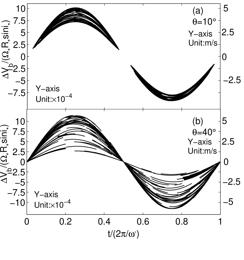
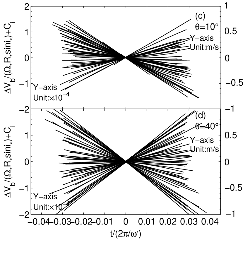
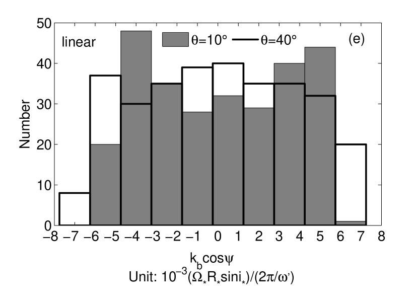
Figure 5: The $\Delta v_{b}$ of the deviation in the R-M effect due to the transit of a binary planet (see eq. 12). Panels (a)–(b) are for the sine mode of $\Delta v_{b}$, and panels (c)–(d) for the linear mode. For each mode, we show the results for different $\theta$. The figure is obtained by full three-body numerical simulations. The related parameters used in the simulations are the same as those in Fig. 3, except $\log(\frac{m_{1}+m_{2}}{m_{*}})=-4$ set for the linear mode and the different values of $\theta$. In each of panels (a)–(d), each curve represents the $\Delta v_{b}$ within one transit event of the binary planet, and multiple curves represent the results of its multiple transit events. We obtain 500 continuous transit events for each system and display only 20% of them (chosen randomly) in those panels for visual clarity. Note that the time span of the transit events is longer than the precession period $2\pi/\Omega$, and a longer time span can give a better statistical illustration in panel (e). Each curve of the transits is different due to the time evolution of the angles $\lambda^{\prime}$ and $i^{\prime}$ and/or different orbital phases $\phi$. All the curves in each panel are stacked up for comparison of either their amplitudes or their slopes. In panels (a) and (b), the curves have been shifted along the $x$-axis to have $\Delta v_{b}=0$ at $t=0$ and have their corresponding maxima/minima aligned; and in panels (c) and (d), the curves have been shifted along the $y$-axis to have their middle points at the zero point, and the constant $C_{i}$ on the $y$-axis labels indicates the shifts, which are different for different events. In each curve, only the complete transit phase is shown with the overlapping period of the two planets being removed for visual clarity, which can be done based on its corresponding transit light curve, although in reality some system information can also be extracted from the ingress, egress, and overlapping parts. The projection of a binary planet is more likely to overlap along the line of sight when $\theta$ is small. The gap in the middle of the curves shown in panel (a) is just the result of removing the overlapping phase of the two planets. As seen from panels (a) and (b), the scatter of the velocity amplitude in the sine modes is larger for the larger angle $\theta=40\arcdeg$ than that for $\theta=10\arcdeg$, which is consistent with the behavior of $f$ shown in Figure 4. Panel (e) gives the slope distributions of the $\Delta v_{b}$–$t$ curves obtained for the linear mode, which also appear different for different $\theta$.

In addition, in some cases, the binary planet are not in the complete transit phase, but only one component is in the transit. For example, this may occur in the ingress or egress phase; and if $d>2R_{*}$, it is also more likely that each component transits in front of the star one by one. In these cases, it is easy to generalize the analysis above and obtain the deviation in the R-M effect due to the transit of each component, by setting the projected area of the other component to zero in the formula above.

Note that in the modeling of most of the other exomoon detection methods, the orbit of the exomoon surrounding the planet is assumed to be co-aligned with the orbit of the planet surrounding the star. Sato & Asada (2010) consider how the special step or overlap features shown in transit light curves (cf., Fig. 3a) can be used to infer the orbital inclination of an exomoon, in which the relevant cases are for the condition that $i^{\prime}$ is close to $90\arcdeg$. The transit duration variations derived by Kipping (2009b) involve the different inclination parameters of an exomoon, but which is limited to $\omega^{\prime}\delta t\ll 1$ or the linear mode and ignores the evolution of the dynamical systems (i.e., the precession of $\vec{n}^{\prime}$).

3.3 Systems likely to be revealed by observations

To have the signatures of a binary planet detectable in observations, the change of the stellar radial velocity anomaly due to the binary planet should be significantly large during each transit. As analyzed above, the deviation $\Delta v_{*}$ is composed of two parts, $\Delta v_{O^{\prime}}$ and $\Delta v_{b}$ (see eq. 10), and both have the contributions from a second planet or exomoon.

For the first part $\Delta v_{O^{\prime}}$, the contribution from each component of the binary can be estimated by

$$\sim 5{\rm m\,s^{-1}}\left(\frac{KR_{*}}{5{\rm km\,s^{-1}}}\right)\left(\frac{10^{3}A_{i}}{A_{*}}\right)\quad i=1,2,$$ (21)

which is the same if the two components have identical projected areas; and the special features (e.g., step change EE^′) shown in Figure 3 have the same orders of magnitude as that estimate and may serve as some characteristic signals of binary planet candidates in the R-M effect.

For the second part $\Delta v_{b}$, which reveals the dynamical configuration of the inner binary, we used some individual systems with specific dynamical parameters to indicate its effect in the above section. Here to see a general parameter space of binary planet systems that are likely to be revealed in $\Delta v_{b}$ by observations, we define the following velocity change:

$$\delta v_{b} \equiv K\left|\frac{d_{1}A_{1}-d_{2}A_{2}}{A_{*}-A_{1}-A_{2}}\right|\omega^{\prime}\delta t,\quad\mbox{if }\omega^{\prime}\delta t<1,$$ (22)

$$\simeq KR_{*}\left(\frac{a}{d}\right)^{1/2}\left(\frac{m_{1}+m_{2}}{m_{*}+m_{1}+m_{2}}\right)^{1/2}\left(\frac{A_{1}+A_{2}}{A_{*}}\right)f_{\delta v_{b}}$$ (23)

and

$$\delta v_{b} \equiv K\left|\frac{d_{1}A_{1}-d_{2}A_{2}}{A_{*}-A_{1}-A_{2}}\right|,\quad\mbox{if }\omega^{\prime}\delta t\geq 1,$$ (24)

$$\simeq KR_{*}\left(\frac{d}{R_{*}}\right)\left(\frac{A_{1}+A_{2}}{A_{*}}\right)f_{\delta v_{b}},$$ (25)

where

$$f_{\delta v_{b}} = \left|\frac{\frac{d_{1}}{d}-\frac{A_{2}}{A_{1}+A_{2}}}{1-\frac{A_{1}+A_{2}}{A_{*}}}\right|,$$ (26)

$$\simeq \left|\frac{1}{1+m_{1}/m_{2}}-\frac{1}{1+\left(\frac{m_{1}/m_{2}}{\rho_{1}/\rho_{2}}\right)^{2/3}}\right|,\quad\mbox{if }\frac{A_{1}+A_{2}}{A_{*}}\ll 1.$$

Equation (22) represents the maximum change of the stellar radial velocity anomaly due to the inner binary in the linear mode of equation (14), i.e., $k_{b}\delta t$; and equation (24) represents the amplitude of the sine mode shown in equation (12). Note that the $\delta v_{b}$ in both equations (22) and (24) is a defined variable. Although the expressions are obtained through the limits at $\omega^{\prime}\delta t\ll 1$ and $\omega^{\prime}\delta t\gg 1$, their values at $\omega^{\prime}\delta t$ should be in the transition of the two limits and the equations above work for the order-of-magnitude estimates and the purpose of the paper. As seen from the equations above, not only the planet areas/sizes are involved in the R-M effect as for a single planet, but their masses or mass densities are also involved in the effect for a binary planet due to the relative motion of the two components of the binary, as the hidden areas of the stellar surface are affected by the relative positions of the binary components and the relative distance of each component from the center of mass of the binary (cf., eqs. 8 and 9) is determined by its two component masses. Given the mass ratios of the two components, the radius ratios can also be expressed through their mass density ratios. Thus, the amplitudes of the R-M effects indicated in Figures 6–8 are expressed through the extra dimensions in multiple panels. The involvement of the extra (mass density) dimension in the study is useful especially considering that recent Kepler observations have revealed the mass density of planets do span a large range. In addition, the R-M effect for the transit of a single planet is related with the orbital semimajor axis, but the semimajor axis $a$ of the outer binary is involved in the effect for a binary planet as shown in equation (23) because the transit time $\delta t$ is affected by $a$ and a longer transit time leads to a larger change of the relative position of the binary components and further a larger deviation in the stellar radial velocity.

As seen from equation (26), the value of $\delta v_{b}$ is significant only if the two components of the binary planets are different, especially if the heavy one has a high mass density and the light one has a low mass density. If the two components have the same mass and mass density, they have the same projecting area and their motion is symmetric, and thus we have $\delta v_{b}=0$ with $f_{\delta v_{b}}=0$, although in this case the contribution from $\Delta v_{O^{\prime}}$ (eq. 11) can be large due to the combination of the projected areas of the two single components. In addition, the value of $\delta v_{b}$ is significant only if the area of the binary planet $A_{1}+A_{2}$ is significantly large, as $\delta v_{b}$ is proportional to $\frac{A_{1}+A_{2}}{A_{*}}$.

By using equations (23) and (25), we show how $\delta v_{b}$ depends on other various properties of the system in Figures 6–7. We set the parameters $KR_{*}=5{\rm km\,s^{-1}}$ and $\frac{A_{1}+A_{2}}{A_{*}}=0.01$ in both of the figures. We set $R_{*}/a=0.005$ and $0.05$ in Figures 6 and 7, respectively. If $R_{*}=R_{\odot}$, $R_{*}/a=0.005$ corresponds to the distance of the earth from the sun ($a=1{\rm AU}$), and $R_{*}/a=0.05$ corresponds to some typical semimajor axis of hot Jupiters discovered in the vicinity of a star ($a=0.1{\rm AU}$). The contours of $\delta v_{b}$ as a function of $(m_{1}+m_{2})/m_{*}$ and $a/d$ are shown by black solid curves. In each figure we display how the contours change for binary planets with different mass ratios ($m_{1}/m_{2}=1.2,10,100,1000$) and different mass density ratios ($\rho_{1}/\rho_{2}=5,1,0.2$). As seen from the figures, in the region below the black dotted curve (i.e., $\omega^{\prime}\delta t<1$), $\delta v_{b}$ increases with increasing $(m_{1}+m_{2})/m_{*}$ and $a/d$, as $\omega^{\prime}\delta t$ does in the same tendency (see eq. 23); and in the region above the curve, $\delta v_{b}$ increases with decreasing $a/d$ (given $R_{*}/a$), as the difference of the line-of-sight rotation velocity of a star covered by each component is likely to be relatively large for a wide binary planet (with large $d$). By comparing the contours obtained for different mass density ratios, the figures also illustrate that the values of $\delta v_{b}$ can be significant (e.g., up to ${\rm m\,s^{-1}}$ or several ten ${\rm m\,s^{-1}}$) only if the two components of the binary planets are different, especially for high $\rho_{1}/\rho_{2}$ ratios (see panels 1a-1c), as analyzed above. Given $\rho_{1}/\rho_{2}$, the $\delta v_{b}$ at bottom panels (e.g., 1d, 2d, 3d) have relatively low values, which indicates the difficulty to detect the effect of a too small exomoon. Figure 7 has a higher $R_{*}/a$ than Figure 6. On the one hand, the curve of $\omega^{\prime}\delta t=1$ in Figure 7 (black dotted curve) shifts downwards; and thus, although the contours of $\delta v_{b}$ below the black dotted curve are the same in both of the figures, the region above the curve has relatively low $\delta v_{b}$ in Figure 7. On the other hand, a higher $R_{*}/a$ would imply a shorter period of the binary rotating around the star and thus a higher probability to do multiple transit observations to get a better statistics for the system. In addition, for different values of $KR_{*}$ and $\frac{A_{1}+A_{2}}{A_{*}}$, the contour values of $\delta v_{b}$ in the figures should be adjusted simply by multiplying them by a factor of $(\frac{KR_{*}}{5{\rm km\,s^{-1}}})\cdot(\frac{A_{1}+A_{2}}{0.01A_{*}})$.

Based on the results above, we discuss the magnitude of the $\delta v_{b}$ in the following examples of binary planet or exomoon systems. We assume that the central star is a solar-like star (with solar mass and radius).

• An earth-moon system (with $m_{1}/m_{2}\simeq 81$, $\rho_{1}/\rho_{2}\simeq 1.6$, $R_{*}/a\simeq 0.005$, $a/d\simeq 400$) may cause a $\delta v_{b}$ only up to $0.1{\rm cm\,s^{-1}}$, e.g., due to the small sizes of the earth and the moon (with $\frac{A_{1}+A_{2}}{A_{*}}\simeq 10^{-4}$), which is too small to be detected. Note that according to the estimate by equation (21), the contribution of the moon to the deviation $\Delta v_{O}^{\prime}$ can be up to $1{\rm cm\,s^{-1}}$ (consistent with the value shown in Simon et al. 2010, where the effect of $\Delta v_{b}$ is not discussed).

• The Ganymede is the biggest moon in the Solar system. A Jupiter-Ganymede system (with $m_{1}/m_{2}\simeq 1.3\times 10^{4}$, $\rho_{1}/\rho_{2}\simeq 0.7$) may lead to a $\delta v_{b}$ only up to several ${\rm cm\,s^{-1}}$ (for $R_{*}/a\simeq 0.001$, $a/d\simeq 800$).

• For a Jupiter-rocky moon system (e.g., with $\rho_{1}/\rho_{2}=0.2$): a moon or satellite with mass $m_{2}<0.1m_{1}$ has a low $\delta v_{b}$ less than ${\rm m\,s^{-1}}$ (cf., panels 3b-3d in Figs. 6–7). A Jupiter-earth system (with $m_{2}\simeq 3\times 10^{-3}m_{1}$) has a low $\delta v_{b}$ only in the range of 1–10${\rm cm\,s^{-1}}$ (see panels 3c-3d). However, if the rocky moon/satellite has a mass close to the Jupiter (see panel 3a), the $\delta v_{b}$ can be up to several to several ten ${\rm m\,s^{-1}}$, which may be detectable by the current techniques. Note that this is an exotic case, as all the rock bodies revealed by the Kepler do not exceed several ten earth mass so far.

• A binary Jupiter-like planet system (e.g., with component masses $m_{1}=10M_{J}$ and $m_{2}=1$ or $0.1M_{J}$, and with Jupiter-like mass densities $\rho_{1}=\rho_{2}$) may have a $\delta v_{b}$ ranging from ${\rm m\,s^{-1}}$ to several ten ${\rm m\,s^{-1}}$, although hot binary Jupiter systems (with relatively high $R_{*}/a$) have relatively low $\delta v_{b}$. The $\delta v_{b}$ can be even larger if $\rho_{1}>\rho_{2}$. For such a system, if any, its signatures on the R-M effect may be detected by future observations.

• The CoRoT-9 system has a solar-like central star and its orbiting exoplanet CoRoT-9b has the mass and radius close to the Jupiter’s. The CoRoT-9b is one of the longest period transiting Jupiter ($\simeq 95$ days) that has so far been confirmed and has a semimajor axis $a\simeq 0.4{\rm AU}$. Its $R_{*}/a\simeq 0.01$ is between the cases shown in Figs. 6 and 7. As inferred from the figures, if the CoRoT-9b has a satellite $m_{2}\gtrsim 10^{-3}m_{1}$, its $\delta v_{b}$ can range from several ${\rm cm\,s^{-1}}$ to several ${\rm m\,s^{-1}}$, depending on the detailed satellite properties.

By using equations (13), (16), (22), and (24), the ratio of the two parts in the deviation $\Delta v_{*}$ (see eq. 10) is about

$$\frac{\delta v_{b}}{k_{O^{\prime}}\delta t}\simeq 0.1\left(\frac{\delta v_{b}}{5{\rm m\,s^{-1}}}\right)\left(\frac{5{\rm km\,s^{-1}}}{KR_{*}}\right)\left(\frac{0.01A_{*}}{A_{1}+A_{2}}\right).$$ (27)

As mentioned above, both of the two parts have the contribution from a second planet or exomoon, and the ratio of the two contributions can be estimated by $(\frac{\delta v_{b}}{5{\rm m\,s^{-1}}})(\frac{5{\rm km\,s^{-1}}}{KR_{*}})(\frac{10^{-3}A_{*}}{A_{i}})$.

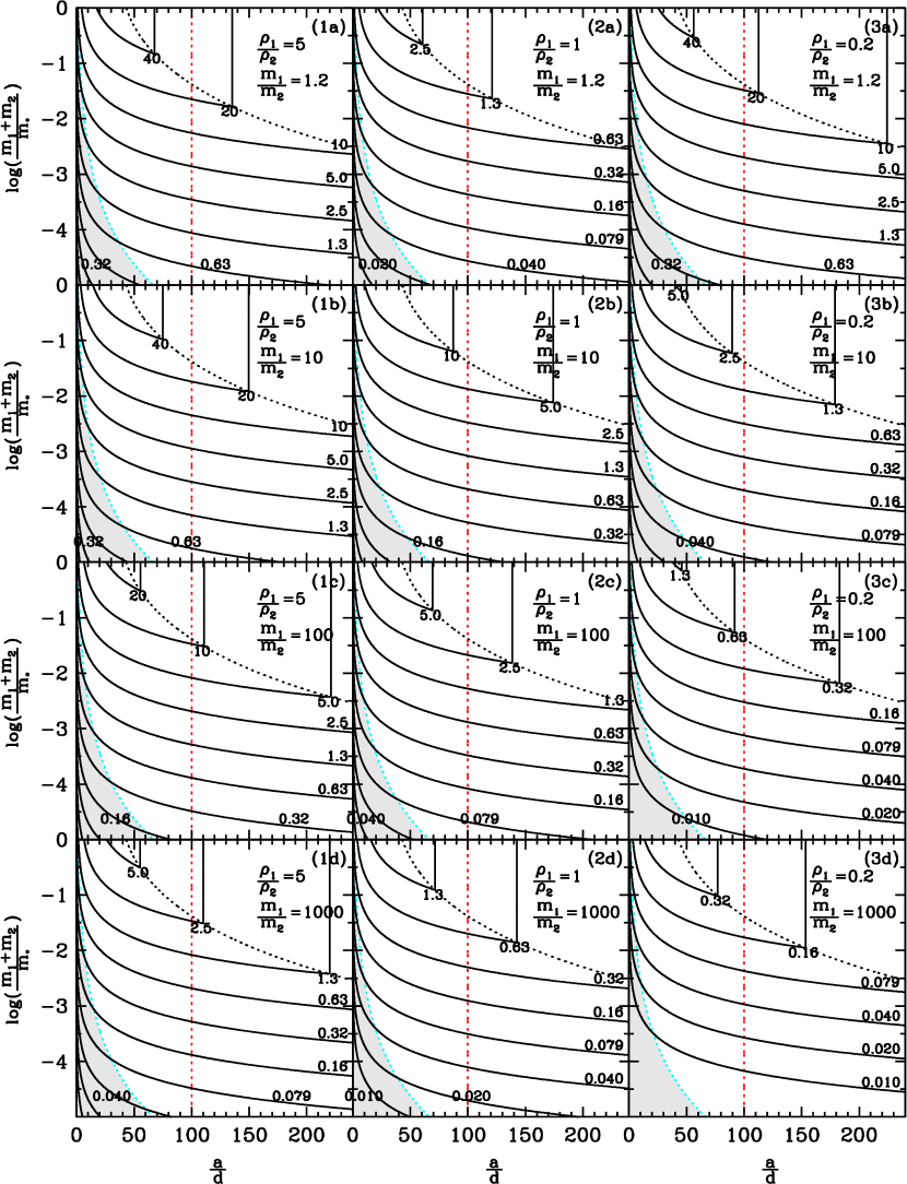
Figure 6: Equi-$\delta v_{b}$ curves for different $\frac{m_{1}+m_{2}}{m_{*}}$ and $a/d$. The contours of $\delta v_{b}$ are drawn in black solid curves and calculated from equations (23) and (25). The values of $\delta v_{b}$ labeled for each curve are in units of ${\rm m\,s^{-1}}$, and they are chosen in an interval of $\Delta\log(\delta v_{b}/{\rm m\,s^{-1}})=0.3$. The cyan dotted curve indicates the Hill radius (eq. 2), and a binary planet with parameters located below the curve cannot survive due to the tidal breakup by the star. The black dotted curve indicates $\omega^{\prime}\delta t=1$, which separates the two regimes expressed by equations (23) and (25). The region below the black dotted curve has $\omega^{\prime}\delta t<1$. The parameters are set as follows: $KR_{*}=5{\rm km\,s^{-1}}$, $\frac{A_{1}+A_{2}}{A_{*}}=0.01$, and $\frac{R_{*}}{a}=0.005$. The red line is a reference line for $d=2R_{*}$. The $\delta v_{b}$ labeled are estimated for a binary in the complete transit phase. Generally a binary located to the left of the red line is more likely not to have the complete transit phase and the transit of each component in front of the star occurs one by one; in this case, the $\delta v_{b}$ can also be easily estimated, and one component may have a larger value than the labeled one and the other component has a smaller value. As labeled in the figure, different panels give different mass and mass density ratios of a binary planet, i.e., $\rho_{1}/\rho_{2}=5$, 1, 0.2 and $m_{1}/m_{2}=1.2$, 10, 100, 1000.

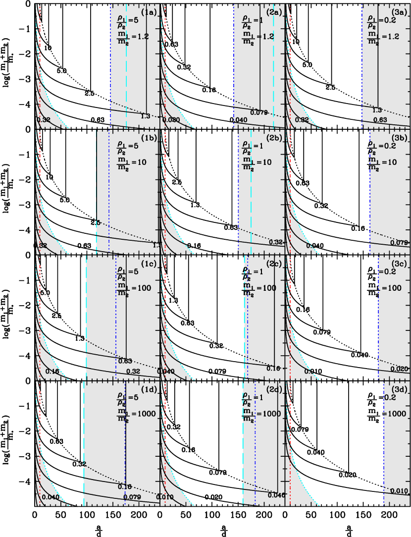
Figure 7: Same as in Figure 6, except that the parameter $\frac{R_{*}}{a}=0.05$ is set in this figure. The cyan dashed line shown in some panels represents the Roche limit, calculated from equation (3); and the parameter space of a binary planet should lie to the left of the line. The blue dotted line is a reference line for $d=R_{1}+R_{2}$, and a binary planet should also lie to the left of the line. As in Figure 6, the grey shaded areas indicate the parameter space that a binary planet cannot survive dynamically. Both the cyan dashed line and the blue dotted line are not shown in Figure 6, as they lie beyond the upper bound of the x-axis of each panel.

Note that a binary planet has a different gravitational effect on the stellar motion from a single planet. The quadrupole moment of the gravitational force from the binary planet is

$$\Delta F\sim\frac{Gm_{*}}{a^{2}}\cdot\frac{m_{1}d_{1}^{2}+m_{2}d_{2}^{2}}{a^{2}},$$ (28)

and its effect on the dynamical motion over each transit duration can be estimated by

$$\frac{\Delta F\delta t}{m_{*}}\sim 1{\rm cm\,s^{-1}}\left(\frac{v_{*}}{100{\rm m\,s^{-1}}}\right)\left(\frac{10d}{a}\right)^{2}\left(\frac{10m_{2}}{m_{1}}\right)\left(\frac{10R_{*}}{a}\right),$$ (29)

which is generally negligible. The $v_{*}$ is the velocity of the star relative to the center of mass of the system. It would be interesting to investigate the long-term dynamical effect of the binary planet on the stellar radial velocity, but which is beyond the scope of this paper.

3.4 Application to hierarchical triple star systems

Figures 6-7 can be applied to a hierarchical triple star system (e.g., for the parameter space $\frac{m_{1}+m_{2}}{m_{*}}\gtrsim 10^{-3}$, in which a dark binary star is transiting in front of a tertiary star (e.g., Carter et al. 2011). Here by “dark” we mean that the light emission from the binary is ignored as planets for simplicity. It is easy to generalize the analysis above to include the light emission from the binary. If the transiting binary is a compact object (e.g., white dwarf or neutron star) plus a planet/brown dwarf, the factor $f_{\delta v_{b}}$ is up to 1, and the $\delta v_{b}$ can be much larger than that of binary planet system. Figure 8 illustrates such a case. As seen from the figure, the $\delta v_{b}$ is high, up to $10^{2}{\rm m\,s^{-1}}$. Thus, such hierarchical triple star systems may be revealed through the R-M effects by future observations.

Figure 9 illustrates two examples of the transit light curves and the radial velocity anomaly curves for the triple star systems with dynamical parameters located in the parameter space shown in Figure 8. As seen from the figure, the radial velocity anomaly caused by the rotational motion of the planet/brown dwarf around the compact object is much more significantly displayed either through the bulge/hill/trough features during the ingress/egress phase (for panel a) or in the sine-like curve during the complete transit phase. The values of $\Delta v_{b}$ can be comparable to $\Delta v_{O^{\prime}}$. It is plausible to expect that the features of these curves are very useful to infer the dynamical configurations of the systems, as illustrated for binary planets above. A more detailed discussion on extracting the configurations is beyond the scope of the paper.

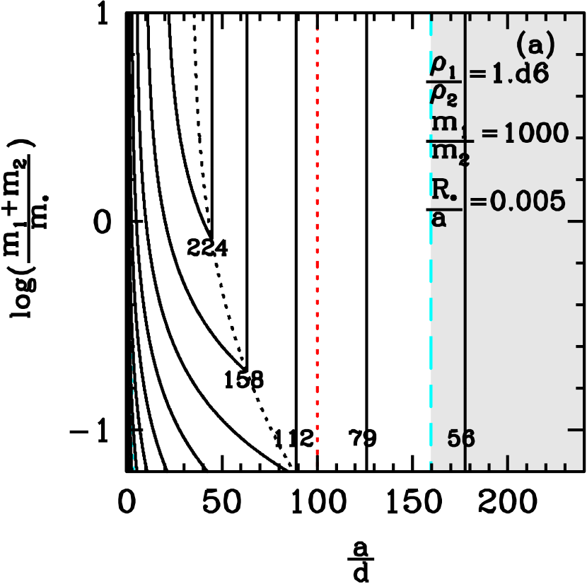
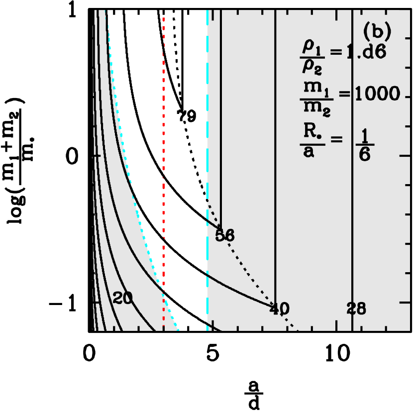
Figure 8: Equi-$\delta v_{b}$ curves for hierarchical triple star systems. The curves have the same meanings as those in Figures 6 and 7. The values of $\delta v_{b}$ labeled for each curve are in an interval of $\Delta\log(\delta v_{b}/{\rm m\,s^{-1}})=0.15$. The binary star in the hierarchical triple star system is composed of a compact object (e.g., white dwarf or neutron star) plus a planet/brown dwarf, so a very high density ratio $\rho_{1}/\rho_{2}$ is used in the figure. The parameters $KR_{*}$ and $\frac{A_{1}+A_{2}}{A_{*}}$ are the same as those in Figure 6. The $R_{*}/a$ is $0.005$ for panel (a) and $1/6$ for panel (b), respectively. As $m_{1}/m_{2}$ decreases, the cyan dashed line shifts rightwards, and the contours of $\delta v_{b}$ are affected little for $m_{1}/m_{2}\gtrsim 10$. See also Section 3.4.

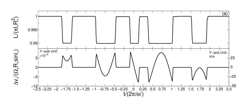
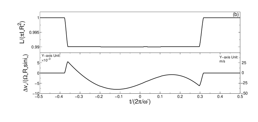
Figure 9: Examples of the simulated transit light curves and the stellar radial velocity anomaly curves for a dark binary star transiting in front of a tertiary star. The methods to obtain the simulated curves are the same as those for Figure 3. The system parameters used in panels (a) and (b) are chosen from the parameter space shown in Figure 8(a) and (b), respectively. Panel (a) has $\log(\frac{m_{1}+m_{2}}{m_{*}})=0$, $a/d=150$, $i=90\arcdeg$, and $\theta=10\arcdeg$; and panel (b) has $\log(\frac{m_{1}+m_{2}}{m_{*}})=0$, $a/d=4$, $i=89.5\arcdeg$, and $\theta=10\arcdeg$. Both of the examples indicate a significant amplitude of changes in the radial velocity anomaly caused by the relative motion between the compact object and the planet/brown dwarf. In panel (a), a number of the bulge/hill/trough features are indicated in the curves, which is because the orbital period of the dark binary is relatively short so that the planet/brown dwarf rotating around the compact star can move completely into, and then move out of, and then re-move into the projected stellar surface before the complete transit phase. The similar effect of the rotational motion also occurs during the egress phase. In panel (b), the sine mode of $\Delta v_{b}$ represented by equation (12) is significantly shown in $\Delta v_{*}$. See also Section 3.4.

4 Discussion

The properties of binary planets (e.g., mass, size, and semimajor axis) can be constrained through their signatures on the transit light curves and stellar radial velocity curves. Our analysis of the R-M effect for a binary planet during its complete transit phase show that effect is composed of two parts. The first part is the conventional one similar to the R-M effect from the transit of a single planet with the combined masses and projected areas of the binary components (eq. 11); and the second part is caused by the orbital rotation of the binary components, which may add a sine- or linear-mode deviation to the stellar radial velocity curve (eq. 12).

In this paper we focus on the discussion on the second part, and we find both the evolution of the orbital rotating phases and the precession of the binary orbital plane may lead to different amplitudes of the deviations in different transit events of the same system. The resulted distribution and dispersion of the deviations in multiple transit events can be used to extract the orbital configuration of the binary planet or even the inclination of its orbital plane relative to the plane of its center of mass rotating around the star (e.g., Fig. 5).

The second part of the R-M effect is more likely to be revealed if the binary components have different masses and mass densities, especially if the heavy one has a high mass density and the light one has a low density. For example, our calculations show that the signature can be up to several or several ten ${\rm m\,s^{-1}}$ with the mass ratio $m_{1}/m_{2}$ up to $10^{3}$, if the mass density ratio $\rho_{1}/\rho_{2}=5$. A small and rocky exomoon with $m_{2}<0.1m_{1}$ would cause a low $\delta v_{b}$ less than ${\rm m\,s^{-1}}$. A strong signature may be caused if at least one of the components of the binary planet is a giant planet. Note that stellar noises produced by oscillations, granulation phenomena, and activities could contribute to the change of stellar radial velocities with an amplitude up to ${\rm m\,s^{-1}}$ (e.g., Dumusque et al. 2011), but they have their own variation periods and patterns to be distinguished from the effect of binary planets, and some statistical methods can be developed to extract smaller signals from the noises.

A long observation time would cover multiple transits of a binary planet, and a better statistics on the distribution of the deviation in the R-M effect could be potentially obtained. To trace the evolution of the geometric configuration of the system, we need at least one period of the orbital angular momentum of the inner binary precessing around that of the outer binary. The precession period is roughly about $\omega^{\prime}/\omega$ times the orbital period of the outer binary. For the parameter space shown in Figures 6 and 7, $\omega^{\prime}/\omega$ is generally less than $200$ (cf., the $\omega^{\prime}\delta t=1$ curve, which can also be taken as a reference line for $\omega^{\prime}/\omega\simeq(R_{*}/a)^{-1}$).

The misalignment between the plane of the binary planet and its rotating plane around the star is one of fundamental parameters of the dynamical system. A large misalignment is likely to cause a large dispersion or different distribution of the deviations in the R-M effect. Recent measurements have discovered that the orbit of a planet may be highly inclined to the stellar spin. Different mechanisms have been proposed for the formation of those misaligned orbits, e.g., Kozai capture, planet-planet scattering, resonance capture by planet migration (e.g., Murray-Clay & Schlichting 2011; Nagasawa et al. 2008; Fabrycky & Tremaine 2007; Yu & Tremaine 2001). Similarly, the different configurations/inclinations of binary planets (see $\theta$ defined in Table 1), if detected in future, should be also useful in constraining formation mechanisms of binary planets or exomoons, and shed new light on our understanding the diversity of planetary systems. For example, different moon formation mechanisms may lead to their different kinematic distributions. Moons formed from the disk material surrounding a planet are predicted to have prograde orbits, while those formed from gravitational capture/impacts/exchange interactions can have either prograde or retrograde orbits (Jewitt & Haghighipour 2007; and references therein). It is also likely that the orbit of a moon could be affected by the later evolution of the system (e.g., by the later inner/outer migration of the outer/inner planets). Regarding a binary planet system with comparable component masses, the study of their formation theory is starting (e.g., Podsiadlowski et al. 2010), and one of the most exciting steps would be to discover a realistic system in observations in the near future.

To discover binary planets and exomoons becomes promising and practical with future developments in instruments, which also lay the foundation for finding the signatures discussed in this paper. For example, planned ground-based surveys such as the Large Synoptic Survey Telescope may detect thousands to tens of thousands of planetary transit candidates; and the space missions, PLAnetary Transits and Oscillations of stars and Transiting Exoplanet Survey Satellite, aim to find transiting planets around relatively bright stars, making it easier to confirm discoveries using follow-up radial velocity measurements. Hopefully follow-up observations could provide some binary planet or exomoon candidates. The astro-comb technique is aiming to achieve a precision as high as $1{\rm cm\,s^{-1}}$ in astronomical radial velocity measurements (Li et al., 2008). Kipping et al. (2012) also proposed a systematic search for exomoons around transiting exoplanet candidates observed by the Kepler mission.

We studied the basic signatures of binary planets that are likely to be revealed in the R-M effect. To understand the roles of the crucial parameters played in the signatures, we have made some approximations in our study, which could be improved or adapted to realistic systems in future work, for example, the study could be extended to a general case in which the center of mass of the binary planet is on an eccentric orbit. The study would become complicated if an exoplanet has multiple moons. In this case, the small moons would contribute little to the deviation in the R-M effect, and the one with a relatively large radius and located at a relatively far distance from the primary planet would imprint the most significant effect. The limb-darkening effect can reduce the amplitude of the R-M effect by 20-40 percent (Simon et al., 2010), and also affect the shape of the radial velocity anomaly (for both the linear and the sine cases studied in this paper). This effect could be corrected with the aid of the observational transit light curves in reality. A statistical method to map the reconstruction of relevant parameters of a binary planet system is beyond the scope of this paper, but would need to be explored in details in future.

After extending the results to a hierarchical triple star system containing a dark binary and a tertiary star, the deviation in the R-M effect would be large enough to be detected especially if the dark binary is composed of a compact object and a brown dwarf/planet, which may put further constraints on the geometrical configuration of triple star systems and provide insights on their formation and evolution.

We thank the referee for many helpful comments. This research was supported in part by the National Natural Science Foundation of China under No. 10973001.

References

- Albrecht et al. (2007) Albrecht, S., Reffert, S., Snellen, I., Quirrenbach, A., & Mitchell, D. S. 2007, A&A, 474, 565
- Carter et al. (2011) Carter, J. A. et al. 2011, Science, 331, 562
- Collier Cameron et al. (2010) Collier Cameron, A. et al. 2010, MNRAS, 407, 507
- Dumusque et al. (2011) Dumusque, X., Udry, S., Lovis, C., Santos, N. C., & Monteiro, M. J. P. F. G. 2010, A&A, 525, A140
- Fabrycky & Tremaine (2007) Fabrycky, D., & Tremaine, S. 2007, ApJ, 669, 1298
- Ford et al. (2000) Ford, E. B., Kozinsky, B., & Rasio, F. A. 2000, ApJ, 535, 385
- Forveille et al. (2011) Forveille, T. et al. 2011, arXiv:1109.2505
- Hirano et al. (2011) Hirano, T., Suto, Y., Winn, J. N., Taruya, A., Narita, N., Albrecht, S., & Sato, B. 2011, ApJ, 742, 69
- Jewitt & Haghighipour (2007) Jewitt, D.,& Haghighipour, N. 2007, ARA&A, 45, 261
- Kipping (2009a) Kipping, D. M. 2009a, MNRAS, 392, 181
- Kipping (2009b) Kipping, D. M. 2009b, MNRAS, 396, 1797
- Kipping et al. (2009) Kipping, D. M., Fossey, S. J., Campanella, G., Schneider, J., Tinetti, G. 2009, in du Foresto V. C., Gelino D. M., Ribas I. eds, ASP Conf. Ser. Vol. 430, Pathways Towards Habitable Planets. Astron. Soc. Pac., San Francisco, p. 139
- Kipping et al. (2012) Kipping, D. M., Bakos, G. Á., Buchhave L., Nesvorný, D., Schmitt, A. 2012, arXiv:1201.0752
- Kozai (1962) Kozai, Y. 1962, ApJ, 67, 591
- Li et al. (2008) Li, C.-H. et al. 2008, Nature, 452, 610
- Lissauer et al. (2011) Lissauer J. J. 2011, Nature, 470, 53
- Lovis et al. (2010) Lovis, C., Ségransan, D., & Mayor, M. et al. 2011, A&A, 528, A112
- McLaughlin (1924) McLaughlin, D. B. 1924, ApJ, 60, 22
- Murray & Dermott (1999) Murray, C. D., & Dermott, S. F. 1999, Solar System Dynamics (Cambridge: Cambridge Univ. Press)
- Murray-Clay & Schlichting (2011) Murray-Clay, R. A., & Schlichting, H. E. 2011, ApJ, 730, 132
- Nagasawa et al. (2008) Nagasawa, M., Ida, S., & Bessho, T. 2008, ApJ, 498, 508
- Ohta, Taruya, & Suto (2005) Ohta, Y., Taruya, A., & Suto, Y. 2005, ApJ, 622, 1118
- Podsiadlowski et al. (2010) Podsiadlowski, P., Rappaport, S., Fregeau, J. M. & Mardling R. A. 2010, arXiv:1007.1418
- Vogt et al. (2011) Vogt, S. S., Butler, R. P., Rivera, E. J., Haghighipour, N., Henry, G. W., Williamson, M. H. 2010, ApJ, 723, 954
- Winn (2010) Winn, J. 2010, Exoplanets, ed. S. Seager (Tucson, AZ: Univ. of Arizona Press), (arXiv:1001.2010)
- Winn et al. (2005) Winn, J. N. et al. 2005, ApJ, 631, 1215
- Winn et al. (2009) Winn, J. N. et al. 2009, ApJ, 703, 99
- Rossiter (1924) Rossiter, R. A. 1924, ApJ, 60, 15
- Sartoretti & Schneider (1999) Sartoretti, P. & Schneider, J. 1999, A&AS, 134, 553
- Sato & Asada (2009) Sato, M. & Asada, H. 2009, PASJ, 61, L29
- Sato & Asada (2010) Sato, M. & Asada, H. 2010, PASJ, 62, 1203
- Sanchis-Ojeda & Winn (2011) Sanchis-Ojeda, R. & Winn, J. N. 2011, ApJ, 743, 61
- Simon et al. (2009) Simon, A. E., Szabó, Gy. M., & Szatmáry, K. 2009, EM&P, 105, 385
- Simon et al. (2010) Simon, A. E., Szabó, Gy. M., Szatmáry, K., & Kiss, L. L. 2010, MNRAS, 406, 2038
- Simon et al. (2012) Simon, A. E., Szabó, Gy. M., Kiss, L. L., & Szatmáry, K. 2012, MNRAS, 419, 164
- Yu & Tremaine (2001) Yu, Q. & Tremaine, S. 2001, AJ, 121, 1736