Absence of Zeros and Asymptotic Error Estimates for Airy and Parabolic Cylinder Functions

Abstract.

We derive WKB approximations for a class of Airy and parabolic cylinder functions in the complex plane, including quantitative error bounds. We prove that all zeros of the Airy function lie on a ray in the complex plane, and that the parabolic cylinder functions have no zeros. We also analyze the Airy and Airy-WKB limit of the parabolic cylinder functions.

1. Introduction and Statement of Results

This paper represents an important first step in our program of proving the linearized stability of the Kerr black hole. The mathematical problem can be framed as showing that solutions of the so-called Teukolsky equation [10, 1] for spin s=2, with smooth compactly supported initial data outside the black hole, decay uniformly on compact sets. The Teukolsky equation separates into an angular and radial ODE. The angular equation involves a Sturm-Liouville operator of the form

$$-\frac{d^{2}}{du^{2}}+W(u)\>.$$

Here the potential $W$ is complex, and thus the operator is not self-adjoint. Following the procedure developed in [2], we seek a spectral representation for this angular operator. Our method for proving such a spectral representation requires detailed information on the eigensolutions. This information can be obtained by “glueing together” approximate solutions and controlling the error using the methods in [3]. One method for obtaining such approximate solutions is to solve the Sturm-Liouville equation

$$\Big{(}-\frac{d^{2}}{du^{2}}+V(u)\Big{)}\phi(u)=0\>,$$ (1.1)

where $V$ is a linear or quadratic polynomial with complex coefficients. The corresponding solutions are Airy and parabolic cylinder functions, respectively. In this paper we analyze properties of these special functions.

Both of these special functions have interesting representations as contour integrals in the complex plane. Since it is difficult to estimate these integral representations directly, we analyze them with stationary phase-like methods (for an introduction to these methods see for example [6, Section 7.7]) to obtain approximate WKB solutions

$$\frac{1}{\sqrt[4]{V}}\>\exp\Big{(}\int^{u}\sqrt{V}\Big{)}$$ (1.2)

with quantitative error bounds. In order to apply the methods in [3], we also need to control the function $y:=\phi^{\prime}/\phi$, which solves the associated Riccati equation

$$y^{\prime}=V-y^{2}\>.$$ (1.3)

For $y$ to be well-behaved, we must show that $\phi$ has no zeros. This motivates our interest in ruling out zeros of the Airy and parabolic cylinder functions.

Apart from being of independent interest, the results obtained here will be used in the forthcoming papers [4, 5].

2. Estimates for Airy Functions

In this section, we assume that $V$ is a linear function,

$$V(u)=a+bu\qquad\text{with}\qquad a,b\in\mathbb{C}\>.$$

Then the Sturm-Liouville equation (1.1) can be solved explicitly in terms of Airy functions,

$$\phi(u)=\mathfrak{A}(z)\qquad\text{where}\qquad z=b^{-\frac{2}{3}}(a+bu)$$

and $\mathfrak{A}$ is a linear combination of the Airy functions $\operatorname{Ai}$ and $\operatorname{Bi}$ (see [8])

$$\mathfrak{A}(z):=-i\sqrt{\pi}\,\big{(}\operatorname{Ai}(z)+i\,\operatorname{Bi}(z)\big{)}$$

(the reason for our specific linear combination is that it has a particularly simple WKB asymptotic form; see (2.4) below). The corresponding solution of the Riccati equation (1.3) is given by

$$y(u)=b^{\frac{1}{3}}\>\frac{\mathfrak{A}^{\prime}(z)}{\mathfrak{A}(z)}\>.$$

Using the integral representations in [8, eqns (9.5.4) and (9.5.5)]

$$\operatorname{Ai}(z) =\frac{1}{2\pi i}\int_{\infty e^{-\pi i/3}}^{\infty e^{\pi i/3}}\exp\left(\frac{t^{3}}{3}-zt\right)dt$$ (2.1)

$$\operatorname{Bi}(z) =\frac{1}{2\pi}\int_{-\infty}^{\infty e^{\pi i/3}}\exp\left(\frac{t^{3}}{3}-zt\right)dt+\frac{1}{2\pi}\int_{-\infty}^{\infty e^{-\pi i/3}}\exp\left(\frac{t^{3}}{3}-zt\right)dt$$ (2.2)

(where $\infty e^{i\varphi}$ refers to the end point of the contour $\lim_{t\rightarrow+\infty}te^{i\varphi}$, etc.), we obtain

$$\mathfrak{A}(z)=\frac{1}{\sqrt{\pi}}\int_{\Gamma}\exp\left(\frac{t^{3}}{3}-zt\right)dt\>,$$ (2.3)

where $\Gamma$ is the contour $\Gamma=-\mathbb{R}^{+}\cup e^{-i\pi/3}\,\mathbb{R}^{+}$. Note that the last integral is finite because the factor $e^{t^{3}/3}$ decays exponentially at both ends of the contour. From the computation

$$\mathfrak{A}^{\prime\prime}(z) =\frac{1}{\sqrt{\pi}}\int_{\Gamma}t^{2}\>\exp\left(\frac{t^{3}}{3}-zt\right)dt$$

$$=\frac{1}{\sqrt{\pi}}\int_{\Gamma}\left(z+\frac{d}{dt}\right)\exp\left(\frac{t^{3}}{3}-zt\right)dt=z\,\mathfrak{A}(z)$$

one immediately verifies that $\mathfrak{A}$ is a solution of the Airy equation.

In the next lemma, we show that $\mathfrak{A}$ can be obtained from $\operatorname{Ai}$ by a rotation in the complex plane.

Lemma 2.1.

For any $z\in\mathbb{C}$,

$$\mathfrak{A}\big{(}e^{-\frac{i\pi}{3}}\,z\big{)}=2\sqrt{\pi}\>e^{-\frac{i\pi}{6}}\>\operatorname{Ai}(-z)\>.$$

Proof.

We perform a change of variables in the integral (2.3),

$$\mathfrak{A}\big{(}e^{-\frac{i\pi}{3}}\,z\big{)} =\frac{1}{\sqrt{\pi}}\int_{\Gamma}\exp\left(\frac{t^{3}}{3}-e^{-\frac{i\pi}{3}}\,zt\right)dt=\left\{\tau=e^{\frac{2\pi i}{3}}\>t\right\}$$

$$=\frac{1}{\sqrt{\pi}}\>e^{-\frac{2\pi i}{3}}\int_{\infty e^{-\pi i/3}}^{\infty e^{\pi i/3}}\exp\left(e^{-2\pi i}\>\frac{\tau^{3}}{3}-e^{-i\pi}\>z\tau\right)d\tau$$

$$=\frac{1}{\sqrt{\pi}}\>e^{-\frac{2\pi i}{3}}\int_{\infty e^{-\pi i/3}}^{\infty e^{\pi i/3}}\exp\left(\frac{\tau^{3}}{3}+z\tau\right)d\tau$$

$$\!\!\overset{\eqref{Airep}}{=}2i\sqrt{\pi}\>e^{-\frac{2\pi i}{3}}\>\operatorname{Ai}(-z)=2\sqrt{\pi}\>e^{-\frac{i\pi}{6}}\>\operatorname{Ai}(-z)\>,$$

giving the result. ∎

2.1. WKB Estimates

Our first goal is to get asymptotic expansions and rigorous estimates of the functions $\mathfrak{A}^{\prime}(z)$ and $\mathfrak{A}(z)$. We expect that for large $z$, the Airy solution should go over to the WKB wave function (1.2) corresponding to the Airy potential $V(z)=z$,

$$\mathfrak{A}_{\text{\tiny{\rm{WKB}}}}(z):=z^{-\frac{1}{4}}\>e^{\frac{2}{3}\,z^{\frac{3}{2}}}\>.$$ (2.4)

Here we define the roots by $z^{\alpha}=\exp(\alpha\log(z))$, where the logarithm has a branch cut along the ray

$$e^{-\frac{i\pi}{3}}\>\mathbb{R}^{+}\>.$$ (2.5)

In the next theorem, we show that with this branch cut, the WKB wave function (2.4) approximates the Airy function $\mathfrak{A}$ for large $z$, with rigorous error bounds.

Theorem 2.2.

Assume that for given $\varepsilon\in(0,\frac{\pi}{6})$,

$$\arg z\not\in\Big{(}-\frac{i\pi}{3}-\varepsilon,-\frac{i\pi}{3}+\varepsilon\Big{)}\mod 2\pi\>.$$ (2.6)

Then

$$\left|\frac{\mathfrak{A}(z)}{\mathfrak{A}_{\text{\tiny{\rm{WKB}}}}(z)}-1\right| \leq\frac{3}{|z|^{\frac{3}{4}}}\>\frac{1}{\sin^{2}(\varepsilon/2)}\left(1+\log^{2}\big{(}1+\sin^{\frac{3}{2}}(\varepsilon/2)\,|z|^{\frac{3}{4}}\big{)}\right)$$ (2.7)

$$\left|\frac{d}{dz}\left(\frac{\mathfrak{A}(z)}{\mathfrak{A}_{\text{\tiny{\rm{WKB}}}}(z)}\right)\right| \leq\frac{2}{|z|^{\frac{7}{4}}}\>\frac{1}{\sin^{3}(\varepsilon/2)}\left(1+\log^{3}\big{(}1+\sin^{\frac{3}{2}}(\varepsilon/2)\,|z|^{\frac{3}{4}}\big{)}\right).$$ (2.8)

Proof.

The assumption (2.6) and our branch convention for the square root imply that the parameter $c$ defined by

$$c=\operatorname{Re}\left(e^{-\frac{i\pi}{3}}\,\sqrt{z}\right)$$ (2.9)

is positive and bounded by (see Figure 1)

$$c\geq|z|^{\frac{1}{2}}\,\sin(\varepsilon/2\big{)}\>.$$ (2.10)

Figure 1. Parameter regions in the complex plane.

Rewriting the argument of the exponential in (2.3) as

$$\frac{t^{3}}{3}-zt=\frac{2}{3}\>z^{\frac{3}{2}}-\sqrt{z}\>\tau^{2}+\frac{\tau^{3}}{3}\qquad\text{with}\qquad\tau:=t+\sqrt{z}\>,$$

we obtain

$$\mathfrak{A}(z) =\frac{1}{\sqrt{\pi}}\int_{e^{-i\pi/6}\,\mathbb{R}}\exp\left(\frac{2}{3}\>z^{\frac{3}{2}}-\sqrt{z}\>\tau^{2}+\frac{\tau^{3}}{3}\right)d\tau$$ (2.11)

$$=\frac{1}{\sqrt{\pi}}\>e^{-\frac{i\pi}{6}}\int_{-\infty}^{\infty}\exp\left(\frac{2}{3}\>z^{\frac{3}{2}}-e^{-\frac{i\pi}{3}}\sqrt{z}\>s^{2}-\frac{is^{3}}{3}\right)ds\>,$$ (2.12)

where in (2.11) we deformed the contour, whereas in the last line we introduced the new integration variable $s=e^{i\pi/6}\,\tau$. Note that in (2.12) the factor $e^{-is^{3}/3}$ is merely a phase, but the quadratic term in the exponent still ensures convergence of the integral in view of (2.9).

If we drop the cubic term in the exponent, the resulting Gaussian integral can be computed to give precisely the WKB wave function,

$$\mathfrak{A}_{\text{\tiny{\rm{WKB}}}}(z)=\frac{1}{\sqrt{\pi}}\>e^{-\frac{i\pi}{6}}\int_{-\infty}^{\infty}\exp\left(\frac{2}{3}\>z^{\frac{3}{2}}-e^{-\frac{i\pi}{3}}\,\sqrt{z}\,s^{2}\right)ds\>.$$

We thus obtain the error term

$$\begin{split}E(z)&:=\mathfrak{A}(z)-\mathfrak{A}_{\text{\tiny{\rm{WKB}}}}(z)\\ &\,=\frac{1}{\sqrt{\pi}}\>e^{-\frac{i\pi}{6}}\int_{-\infty}^{\infty}\exp\left(\frac{2}{3}\>z^{\frac{3}{2}}-e^{-i\pi/3}\sqrt{z}\>s^{2}\right)\left(e^{-\frac{is^{3}}{3}}-1\right)ds\>.\end{split}$$ (2.13)

After estimating the error term by

$$\left|\sqrt{\pi}\>e^{-\frac{2}{3}\,z^{\frac{3}{2}}}\>E(z)\right|\leq\int_{-\infty}^{\infty}e^{-cs^{2}}\left|e^{-\frac{is^{3}}{3}}-1\right|ds\>,$$

we decompose the integral into integrals over the regions $[-L,L]$ and $\mathbb{R}\setminus[-L,L]$. We bound these integrals as follows,

$$\int_{\mathbb{R}\setminus[-L,L]}e^{-cs^{2}}\left|e^{-\frac{is^{3}}{3}}-1\right|ds \leq 2\int_{\mathbb{R}\setminus[-L,L]}e^{-cs^{2}}\>ds$$

$$\leq 2\,e^{-\frac{cL^{2}}{2}}\int_{-\infty}^{\infty}e^{-\frac{cs^{2}}{2}}\>ds=\frac{2\sqrt{2\pi}}{\sqrt{c}}\,e^{-\frac{cL^{2}}{2}}$$ (2.14)

$$\int_{-L}^{L}e^{-cs^{2}}\left|e^{-\frac{is^{3}}{3}}-1\right|ds \leq 2\int_{0}^{L}\frac{s^{3}}{3}\>ds\leq\frac{L^{4}}{6}\>,$$ (2.15)

where in the last line we used that for all $x\in\mathbb{R}$ the inequality $|e^{ix}-1|\leq|x|$ holds. In order to make both errors of about the same size, we choose

$$L=\sqrt{\frac{2}{c}}\>\log^{\frac{1}{2}}\big{(}1+c^{\frac{3}{2}}\big{)}\>.$$ (2.16)

We thus obtain

$$\left|e^{-\frac{2}{3}\,z^{\frac{3}{2}}}\>E(z)\right|\leq\frac{2^{\frac{3}{2}}}{c^{2}}+\frac{2}{3\,\sqrt{\pi}}\>\frac{1}{c^{2}}\>\log^{2}\big{(}1+c^{3/2}\big{)}\leq\frac{3}{c^{2}}\left(1+\log^{2}\big{(}1+c^{3/2}\big{)}\right).$$

Applying (2.10) and (2.4) gives (2.7).

In order to derive (2.8), we introduce the abbreviations

$$I(z) =\int_{-\infty}^{\infty}\exp\left(-e^{-\frac{i\pi}{3}}\sqrt{z}\>s^{2}-\frac{is^{3}}{3}\right)ds$$ (2.17)

$$I_{\text{\tiny{\rm{WKB}}}}(z) =\int_{-\infty}^{\infty}\exp\left(-e^{-\frac{i\pi}{3}}\,\sqrt{z}\,s^{2}\right)ds=e^{\frac{i\pi}{6}}\>\sqrt{\pi}\>z^{-\frac{1}{4}}\>.$$ (2.18)

Then

$$\frac{d}{dz}\left(\frac{\mathfrak{A}(z)}{\mathfrak{A}_{\text{\tiny{\rm{WKB}}}}(z)}\right)=\frac{d}{dz}\left(\frac{I(z)}{I_{\text{\tiny{\rm{WKB}}}}(z)}\right)=\frac{I^{\prime}(z)-I^{\prime}_{\text{\tiny{\rm{WKB}}}}(z)}{I_{\text{\tiny{\rm{WKB}}}}(z)}+\frac{I_{\text{\tiny{\rm{WKB}}}}^{\prime}(z)}{I_{\text{\tiny{\rm{WKB}}}}(z)}\>\frac{\mathfrak{A}_{\text{\tiny{\rm{WKB}}}}(z)-\mathfrak{A}(z)}{\mathfrak{A}_{\text{\tiny{\rm{WKB}}}}(z)}\>.$$

Using (2.18) and (2.7), the second summand is estimated by

$$\left|\frac{I_{\text{\tiny{\rm{WKB}}}}^{\prime}(z)}{I_{\text{\tiny{\rm{WKB}}}}(z)}\>\frac{\mathfrak{A}_{\text{\tiny{\rm{WKB}}}}(z)-\mathfrak{A}(z)}{\mathfrak{A}_{\text{\tiny{\rm{WKB}}}}(z)}\right|\leq\frac{1}{|z|^{\frac{7}{4}}}\>\frac{1}{\sin^{2}(\varepsilon/2)}\left(1+\log^{2}\big{(}1+\sin^{\frac{3}{2}}(\varepsilon/2)|z|^{\frac{3}{4}}\big{)}\right).$$ (2.19)

In order to estimate the first summand, we differentiate (2.17) and (2.18) to obtain, similar to (2.13), the identity

$$\sqrt{z} \left(I^{\prime}(z)-I_{\text{\tiny{\rm{WKB}}}}^{\prime}(z)\right)=\int_{-\infty}^{\infty}\left(-\frac{1}{2}\>e^{-\frac{i\pi}{3}}\,s^{2}\right)\exp\left(-e^{-\frac{i\pi}{3}}\sqrt{z}\>s^{2}\right)\left(e^{-\frac{is^{3}}{3}}-1\right)ds\>.$$

It follows that

$$\left|\sqrt{z}\,\big{(}I^{\prime}(z)-I_{\text{\tiny{\rm{WKB}}}}^{\prime}(z)\big{)}\right|\leq\frac{1}{2}\int_{-\infty}^{\infty}s^{2}\>e^{-cs^{2}}\left|e^{-\frac{is^{3}}{3}}-1\right|ds\>.$$

Estimating the integral exactly as in (2.14) and (2.15), we obtain

$$\frac{1}{2}\int_{-\infty}^{\infty}s^{2}\>e^{-cs^{2}}\left|e^{-\frac{is^{3}}{3}}-1\right|ds\leq\frac{\sqrt{\pi}}{c^{\frac{3}{2}}}\,e^{-\frac{cL^{2}}{2}}+\frac{L^{6}}{18}\>.$$

Choosing $L$ again according to (2.16), we obtain

$$\left|\sqrt{z}\,\big{(}I^{\prime}(z)-I_{\text{\tiny{\rm{WKB}}}}^{\prime}(z)\big{)}\right| \leq\frac{1}{\sqrt{\pi}\>c^{3}}\left(1+\log^{3}(1+c^{\frac{3}{2}})\right)\>.$$

Applying (2.18) and (2.10), we conclude that

$$\left|\frac{I^{\prime}(z)-I^{\prime}_{\text{\tiny{\rm{WKB}}}}(z)}{I_{\text{\tiny{\rm{WKB}}}}(z)}\right|\leq\frac{1}{|z|^{\frac{7}{4}}}\>\frac{1}{\sin^{3}(\varepsilon/2)}\left(1+\log^{3}\big{(}1+\sin^{\frac{3}{2}}(\varepsilon/2)\,|z|^{\frac{3}{4}}\big{)}\right).$$

Noting that this contribution dominates (2.19), we obtain (2.8). ∎

In particular, this theorem allows us to take the limit as $z$ goes to infinity along a ray through the origin, as long as we stay away from the branch cut (2.5).

Corollary 2.3.

Let $z_{0}\in\mathbb{C}$ be off the ray $e^{-\frac{i\pi}{3}}\mathbb{R}^{+}$. Then

$$\lim_{t\rightarrow\infty}t^{-\frac{1}{2}}\,\frac{\mathfrak{A}^{\prime}(tz_{0})}{\mathfrak{A}(tz_{0})}=\sqrt{z_{0}}\>,$$

where we again used the sign convention for the square root introduced just before (2.5).

Proof.

We choose $\varepsilon$ so small that $z_{0}$ satisfies the condition (2.6). Then

$$\lim_{t\rightarrow\infty}t^{-\frac{1}{2}}\,\frac{\mathfrak{A}^{\prime}(tz_{0})}{\mathfrak{A}(tz_{0})}=\lim_{t\rightarrow\infty}t^{-\frac{1}{2}}\,\frac{\mathfrak{A}_{\text{\tiny{\rm{WKB}}}}^{\prime}(tz_{0})}{\mathfrak{A}_{\text{\tiny{\rm{WKB}}}}(tz_{0})}\>,$$

and computing $\mathfrak{A}^{\prime}_{\text{\tiny{\rm{WKB}}}}$ from (2.4) gives the result. ∎

2.2. An Estimate for the Riccati Equation for a Complex Potential

Our next goal is to show that the Airy function $\mathfrak{A}$ has no zeros except on the branch cut (2.5). In preparation for this, we now derive an estimate for solutions of the Riccati equation for a general potential $V$ with $\operatorname{Im}V\geq 0$. Thus let $y$ be a solution of the Riccati equation (1.3). Decomposing $y$ into its real and imaginary parts, $y=\alpha+i\beta$, we obtain the system

$$\alpha^{\prime} =\operatorname{Re}V-\alpha^{2}+\beta^{2}$$ (2.20)

$$\beta^{\prime} =\operatorname{Im}V-2\alpha\beta\>.$$ (2.21)

Moreover, we set

$$\sigma=\exp\left(2\int^{u}\alpha\right)\>.$$ (2.22)

Let us assume that $\operatorname{Im}V\geq 0$ on an interval $[u_{0},u_{1}]$ and that $(\alpha,\beta)$ is a solution on a closed subinterval $[u_{0},u_{2}]\subset[u_{0},u_{1}]$. If $\beta(u_{0})>0$, it follows immediately from (2.21) that $\beta>0$ on the whole interval $[u_{0},u_{2}]$. A short calculation yields

$$(\sigma\beta)^{\prime}(u)=\sigma\operatorname{Im}V\geq 0\>.$$

Hence the function $\sigma\beta$ is monotone increasing and

$$\beta(u)\geq\beta_{0}\,\sigma_{0}\>\frac{1}{\sigma(u)}\>,$$

where $\beta_{0}=\beta(u_{0})$ and similarly for all other functions. Using this inequality in (2.20), we obtain

$$\alpha^{\prime}\geq\operatorname{Re}V-\alpha^{2}+\frac{\beta_{0}^{2}\,\sigma_{0}^{2}}{\sigma(u)^{2}}\>.$$ (2.23)

Integrating this inequality gives the following estimate.

Lemma 2.4.

Assume that $\operatorname{Im}V\geq 0$ on the interval $[u_{0},u_{1}]$ and that $(\alpha,\beta)$ is a solution on a closed subinterval $[u_{0},u_{2}]\subset[u_{0},u_{1}]$ with $\beta(u_{0})>0$. Then the function $\alpha$ satisfies the upper bound

$$\alpha(u)\leq g(u)\qquad\text{on~{}$[u_{0},u_{2}]$}\>,$$

where we set

$$g(u)=\frac{\sqrt{C}\sinh(x)+\alpha(u_{2})\,\cosh(x)}{\cosh(x)+\alpha(u_{2})\,\sinh(x)/\sqrt{C}}$$

and

$$C=\inf_{[u_{0},u_{1}]}\operatorname{Re}V\in\mathbb{R}\>,\qquad x=\sqrt{C}\,(u-u_{1})\>.$$

Proof.

Dropping the last summand in (2.23), we obtain the inequality

$$\alpha^{\prime}\geq C-\alpha^{2}\>.$$

Then $\alpha\leq g$, where $g$ is the solution of the corresponding differential equation

$$g^{\prime}=C-g^{2}\>,\qquad g(u_{2})=\alpha(u_{2})\>.$$

Solving this differential equation gives the result. ∎

Using the result of this lemma in (2.22), we get

$$\sigma(u)=\sigma_{0}\,\exp\left(2\int_{u_{0}}^{u}\alpha\right)\leq\sigma_{0}\,\exp\left(2\int_{u_{0}}^{u}g\right).$$

Computing the integral, we obtain

$$\sigma(u)\leq\sigma_{0}\>\left(\frac{\sqrt{C}\cosh\big{(}\sqrt{C}(u-u_{2})\big{)}+\alpha(u_{2})\,\sinh\big{(}\sqrt{C}(u-u_{2})\big{)}}{\sqrt{C}\cosh\big{(}\sqrt{C}(u-u_{0})\big{)}+\alpha(u_{2})\,\sinh\big{(}\sqrt{C}(u-u_{0})\big{)}}\right)^{2}.$$

Using this estimate in (2.23) and setting $u=u_{2}$ gives the following result.

Proposition 2.5.

Assume that $\operatorname{Im}V\geq 0$ on $[u_{0},u_{1}]$ and that $\beta(u_{0})>0$. Assume furthermore that the solution $(\alpha,\beta)$ exists on the interval $[u_{0},u]\subset[u_{0},u_{1}]$ and that $\alpha^{\prime}(u)\leq 0$. Then

$$0\geq C-\alpha(u)^{2}+\beta_{0}^{2}\left[\cosh\big{(}\sqrt{C}(u-u_{0})\big{)}+\frac{\alpha(u)}{\sqrt{C}}\>\sinh\big{(}\sqrt{C}(u-u_{0})\big{)}\right]^{4}\>.$$

Corollary 2.6.

Assume that either $\operatorname{Im}V|_{[u_{0},u_{1}]}\geq 0$ and $\beta(u_{0})>0$ or $\operatorname{Im}V|_{[u_{0},u_{1}]}\leq 0$ and $\beta(u_{0})<0$. Then the solution $(\alpha,\beta)$ exists and is bounded on the interval $[u_{0},u_{1}]$.

Proof.

It suffices to consider the case $\operatorname{Im}V|_{[u_{0},u_{1}]}\geq 0$ and $\beta(u_{0})>0$ because the other case is obtained by taking the complex conjugate of the Riccati equation (1.3).

Let us assume conversely that the solution $(\alpha,\beta)$ blows up at a point $u_{2}\in[u_{0},u_{1}]$. We can assume that $\alpha$ blows up, because otherwise $\beta$ could be obtained by integrating (2.21),

$$\beta(u)=e^{-2\int_{u_{0}}^{u}\alpha}\,\beta(u_{0})+\int_{u_{0}}^{u}e^{-2\int_{\tau}^{u}\alpha}\operatorname{Im}V(\tau)\>d\tau\>.$$ (2.24)

Assume that $\alpha$ tends to $+\infty$. Then (2.24) shows that $\beta$ stays bounded, and thus the right hand side of (2.20) tends to $-\infty$, a contradiction. On the other hand, if $\alpha$ is unbounded from below, then there is a sequence $v_{n}\in[u_{0},u_{2})$ with $\alpha(v_{n})\rightarrow-\infty$ and $\alpha^{\prime}(v_{n})\leq 0$. This contradicts Proposition 2.5. ∎

2.3. Locating the Zeros of the Airy Function

Our method for ruling out zeros of the Airy function $\mathfrak{A}$ at a given point $z_{0}\in\mathbb{C}$ is to consider the Airy function along straight lines of the form

$$z(u)=z_{0}+\lambda u\qquad\text{with}\qquad u\in\mathbb{R}\>,$$ (2.25)

where $\lambda$ is a complex parameter. Then the function $\phi(u):=\mathfrak{A}(z(u))$ satisfies the Sturm-Liouville equation (1.1) with

$$V(u)=\lambda^{2}\;(z_{0}+\lambda u)\>.$$

Applying Corollary 2.6 to the corresponding Riccati solution $y:=\phi^{\prime}/\phi$ yields the following proposition. This proposition follows immediately from Lemma 2.1 and the fact that the function $\operatorname{Ai}$ only has zeros on the negative real axis (see [8, §9.9(i)]). Nevertheless, we present a proof in order to illustrate the methods of Section 2.2 in a simple example (these methods will be used again in Section 3.2).

Proposition 2.7.

The function $\mathfrak{A}$ has no zeros off the ray $e^{-i\pi/3}\,\mathbb{R}^{+}$.

Proof.

Let $z_{0}$ be a point off the ray $e^{-i\pi/3}\,\mathbb{R}^{+}$. We choose $\lambda$ such that $(-\lambda)$ is also off the ray $e^{-i\pi/3}\,\mathbb{R}^{+}$. Then Corollary 2.3 applies and yields

$$\lim_{u\rightarrow-\infty}|u|^{-\frac{1}{2}}\,y(u)=\lambda\lim_{u\rightarrow-\infty}|u|^{-\frac{1}{2}}\,\frac{\mathfrak{A}^{\prime}(z(u))}{\mathfrak{A}(z(u))}=\lambda\>\sqrt{-\lambda}\>.$$

Using our sign convention for the square root, we may choose $\lambda$ such that

$$\sqrt{-\lambda}=e^{i\varphi}\qquad\text{with}\qquad\varphi\in\Big{(}\frac{\pi}{6},\frac{\pi}{3}\Big{)}\cup\Big{(}\frac{\pi}{3},\frac{\pi}{2}\Big{)}\>;$$ (2.26)

then

$$\lim_{u\rightarrow-\infty}|u|^{-\frac{1}{2}}\,y(u)=-e^{3i\varphi}$$ (2.27)

(note that the parameter $-\lambda=e^{2i\varphi}$ is indeed off the ray $e^{-i\pi/3}\,\mathbb{R}^{+}$ because $\pi/3$ is excluded in (2.26)). Moreover,

$$\operatorname{Im}V(u)=\operatorname{Im}(\lambda^{2}z_{0})+u\operatorname{Im}(\lambda^{3})=\operatorname{Im}(e^{4i\varphi}z_{0})-u\operatorname{Im}(e^{6i\varphi})\>.$$ (2.28)

In the considered range of $\varphi$, the imaginary parts of $e^{3i\varphi}$ and $e^{6i\varphi}$ have opposite signs (see Figure 2).

Figure 2. Admissible phases.

As a consequence, one sees from (2.27) and (2.28) that for sufficiently large negative $u$, the functions $\operatorname{Im}y$ and $\operatorname{Im}V$ are non-zero and have the same sign. Moreover, we can choose $\varphi$ such that the imaginary parts of $e^{4i\varphi}z_{0}$ and $e^{6i\varphi}$ have the same sign (see Figure 2). We conclude from (2.28) that the imaginary part of $V$ has fixed sign on the interval $(\infty,0]$. Thus Corollary 2.6 shows that $y(u)$ is bounded on the interval $(-\infty,0]$. Hence the corresponding Sturm-Liouville solution $\phi(u)=\exp(\int^{u}y)$ has no zeros on this interval. In particular, we conclude that $0\neq\phi(0)=\mathfrak{A}(z_{0})$. ∎

3. Estimates for Parabolic Cylinder Functions

We now consider a quadratic potential

$$V(u)=\alpha+\frac{\beta}{4}\>(u-\gamma)^{2}\qquad\text{with}\qquad\alpha,\beta,\gamma\in\mathbb{C}\>.$$

The corresponding differential equation (1.1) can be solved explicitly in terms of the parabolic cylinder function, as we now recall. The parabolic cylinder function, which we denote by $U_{a}(z)$, is a solution of the differential equation

$$U_{a}^{\prime\prime}(z)=\Big{(}\frac{z^{2}}{4}\>+a\Big{)}\,U_{a}(z)\>.$$ (3.1)

Setting

$$\phi(u)=U_{a}(z)\qquad\text{with}\qquad a=\frac{\alpha}{\sqrt{\beta}}\>,\quad z=\beta^{\frac{1}{4}}\,(u-\gamma)\>,$$

a short calculation shows that $\phi$ indeed satisfies (1.1).

According to [8, §12.5(ii)], particular solutions of (3.1) can be written as contour integrals,

$$U_{a}^{\pm}(z)=e^{-\frac{z^{2}}{4}}\int_{\Gamma_{\pm}}e^{zt-\frac{t^{2}}{2}}\>t^{a-\frac{1}{2}}\>dt\>.$$ (3.2)

We consider the special solution obtained by choosing

$$\Gamma_{\pm}=\mathbb{R}\pm i$$

as the contour from $-\infty\pm i$ to $\infty\pm i$, where we take the usual convention $t^{a-\frac{1}{2}}=\exp((a-\frac{1}{2})\log t)$, and the logarithm has its branch cut along the negative real axis. Whenever we omit the indices $\pm$, our arguments apply to both cases. It is verified by a direct computation that $U_{a}$ satisfies (3.1); namely,

$$U_{a}^{\prime}(z) =\int_{\Gamma}\left(-\frac{z}{2}+t\right)e^{-\frac{z^{2}}{4}+zt-\frac{t^{2}}{2}}\>t^{a-\frac{1}{2}}\>dt$$

$$U_{a}^{\prime\prime}(z) =\int_{\Gamma}\left(\frac{z^{2}}{4}-\frac{1}{2}-t\,(z-t)\right)e^{-\frac{z^{2}}{4}+zt-\frac{t^{2}}{2}}\>t^{a-\frac{1}{2}}\>dt$$

$$=\int_{\Gamma}\>t^{a-\frac{1}{2}}\left(\frac{z^{2}}{4}-\frac{1}{2}-t\,\frac{\partial}{\partial t}\right)e^{-\frac{z^{2}}{4}+zt-\frac{t^{2}}{2}}\>dt$$

$$=\int_{\Gamma}\left(\frac{z^{2}}{4}-\frac{1}{2}+\Big{(}a+\frac{1}{2}\Big{)}\right)\>t^{a-\frac{1}{2}}e^{-\frac{z^{2}}{4}+zt-\frac{t^{2}}{2}}\>dt=\Big{(}\frac{z^{2}}{4}\>+a\Big{)}\,U_{a}(z)\>,$$

where in the last line we integrated by parts.

In the special cases

$$a=\frac{1}{2}\>,\frac{3}{2},\frac{5}{2},\ldots\>,$$ (3.3)

the integral (3.2) is Gaussian and can easily be computed in closed form (giving the well-known eigensolutions of the harmonic oscillator). Therefore, we may restrict attention to the case when (3.3) is violated. As (3.1) only involves $z^{2}$, it is obvious that $U_{a}(-z)$ is also a parabolic cylinder function. Indeed, by a change of variables we see that

$$U_{a}^{+}(-z) =e^{-\frac{z^{2}}{4}}\int_{\Gamma_{+}}e^{-zt-\frac{t^{2}}{2}}\>t^{a-\frac{1}{2}}\>dt=\left\{\tau=-t\right\}$$

$$=e^{-\frac{z^{2}}{4}}\int_{\Gamma_{-}}e^{z\tau-\frac{\tau^{2}}{2}}\>(-\tau)^{a-\frac{1}{2}}\>d\tau\>.$$

Using that $\log(-\tau)=\log(\tau)-i\pi$, we obtain the relation

$$U_{a}^{+}(-z)=e^{-i\pi(a-\frac{1}{2})}\>U_{a}^{-}(z)\>.$$ (3.4)

Moreover, an elementary computation shows that

$$\begin{split}U_{a}^{+}(0)&=2^{a-\frac{1}{2}}\>(1-ie^{i\pi a})\>\Gamma\Big{(}\frac{a}{2}+\frac{1}{4}\Big{)}\\ (U_{a}^{+})^{\prime}(0)&=2^{a+\frac{1}{2}}\>(1+ie^{i\pi a})\>\Gamma\Big{(}\frac{a}{2}+\frac{3}{4}\Big{)}\>.\end{split}$$ (3.5)

Thus the Wronskian of $U_{a}^{+}$ and $U_{a}^{-}$ is given by

$$w(U_{a}^{+},U_{a}^{-}) \overset{\eqref{Uapmrel}}{=}2e^{i\pi(a-\frac{1}{2})}(U_{a}^{+})^{\prime}(0)\>U_{a}^{+}(0)$$

$$\;=e^{i\pi(a-\frac{1}{2})}\>2^{2a+1}\>(1+e^{2i\pi a})\>\Gamma\Big{(}\frac{a}{2}+\frac{1}{4}\Big{)}\>\Gamma\Big{(}\frac{a}{2}+\frac{3}{4}\Big{)}\>.$$

From these formulas, one sees that $U_{a}^{+}$ and $U_{a}^{-}$ are linearly independent except in the trivial cases (3.3) (note that for the values $a=-\frac{1}{2},-\frac{3}{2},\ldots$, the poles of the $\Gamma$ functions in (3.5) are cancelled by the zeros of the corresponding factors $(1\pm ie^{i\pi a})$).

3.1. WKB Estimates

Integral representations for parabolic cylinder function have been used to derive asymptotic expansions (see for example [7] and [9]). The goal of this section is to derive rigorous estimates with quantitative error bounds which go beyond [7, 9] and show that in a certain parameter range, the function $U_{a}(z)$ is well-approximated by a WKB wave function. More precisely, the WKB wave function (1.2) becomes

$$\begin{split}\phi_{\text{\tiny{\rm{WKB}}}}(z)&=\left(\frac{4}{z^{2}+4a}\right)^{\frac{1}{4}}\exp\left(\frac{1}{2}\int^{z}\sqrt{\zeta^{2}+4a}\;d\zeta\right)\\ &=\frac{\big{(}z+\sqrt{z^{2}-b+2}\,\big{)}^{\frac{1}{2}-\frac{b}{4}}}{(z^{2}-b+2)^{\frac{1}{4}}}\>\exp\left({\frac{z}{4}\>\sqrt{z^{2}-b+2}}\right),\end{split}$$ (3.6)

where we introduced the abbreviation

$$b=-4\,\Big{(}a-\frac{1}{2}\Big{)}\>.$$

We write the parabolic cylinder function as

$$U_{a}(z)=e^{-\frac{z^{2}}{4}}\int_{\Gamma}e^{f(t)}\>dt\>,$$ (3.7)

where the function $f$ and its derivatives are given by

$$f(t) =zt-\frac{t^{2}}{2}-\frac{b}{4}\>\log t\>, f^{\prime}(t) =z-t-\frac{b}{4t}$$ (3.8)

$$f^{\prime\prime}(t) =-1+\frac{b}{4t^{2}}\>, f^{\prime\prime\prime}(t) =-\frac{b}{2t^{3}}\>.$$ (3.9)

The zeros of $f^{\prime}$ are computed to be

$$t_{\pm}=\frac{1}{2}\left(z\pm\sqrt{z^{2}-b}\right).$$ (3.10)

We choose $t_{0}$ equal to either $t_{+}$ or $t_{-}$. As we excluded the special cases (3.3), we know that $b\neq 0$ and thus $t_{\pm}\neq 0$.

In order to obtain a “stationary phase-type” approximation to $U_{a}$, we let $\tilde{f}$ be the quadratic Taylor approximation of $f$,

$$\tilde{f}(t)=f(t_{0})+\frac{f^{\prime\prime}(t_{0})}{2}\>(t-t_{0})^{2}\>.$$

It is convenient to introduce the parametrization

$$t=t_{0}\,(1+\tau)\>;$$ (3.11)

then

$$f(t)-f(t_{0}) =-\frac{t_{0}^{2}}{2}\>\tau^{2}+\frac{b}{4}\,\big{(}\tau-\log(1+\tau)\big{)}$$ (3.12)

$$\tilde{f}(t)-f(t_{0}) =\left(-\frac{t_{0}^{2}}{2}+\frac{b}{8}\right)\tau^{2}\>.$$ (3.13)

The coefficient of $\tau^{2}$ in (3.12) is given by

$$d:=-\frac{t_{0}^{2}}{2}=-\frac{1}{8}\left(z\pm\sqrt{z^{2}-b}\right)^{2}\>.$$ (3.14)

We now deform the contour $\Gamma$ to the the straight line

$$\tau(u)=e^{i\alpha}\,u\qquad\text{with~{}$u\in\mathbb{R}$ and~{}$\alpha\in[0,\pi)$}\>.$$ (3.15)

Then

$$g(u)\; \!\!:=\tau(u)-\log\big{(}1+\tau(u)\big{)}=e^{i\alpha}u-\log(1+e^{i\alpha}u)$$

$$=\int_{0}^{u}\frac{d}{ds}\Big{(}e^{i\alpha}s-\log(1+e^{i\alpha}s)\Big{)}\,ds=\int_{0}^{u}\Big{(}e^{i\alpha}-\frac{e^{i\alpha}}{1+e^{i\alpha}s}\Big{)}\,ds$$

$$=\int_{0}^{u}\frac{e^{2i\alpha}s}{1+e^{i\alpha}s}\>ds=\int_{0}^{u}\frac{e^{2i\alpha}s\>(1+e^{-i\alpha}s)}{|1+e^{i\alpha}s|^{2}}\>ds=\int_{0}^{u}\frac{e^{2i\alpha}s+e^{i\alpha}s^{2}}{1+s^{2}+2s\cos\alpha}\>ds$$

$$=e^{2i\alpha}I_{1}(u)+e^{i\alpha}I_{2}(u)\>,$$

where $I_{1}$ and $I_{2}$ are the real-valued functions

$$I_{\ell}(u)=\int_{0}^{u}\frac{s^{\ell}}{1+s^{2}+2s\cos\alpha}\>ds\>,\qquad\ell=1,2\>.$$ (3.16)

Choosing a polar decomposition of $b$ and $d$,

$$b=|b|\,e^{i\beta}\>,\quad d=|d|\,e^{i\delta}\qquad\text{with~{}$\beta,\delta\in[-\pi,\pi]$}\>,$$

and introducing the abbreviation

$$\rho=\left|\frac{b}{8d}\right|,$$ (3.17)

we obtain

$$\operatorname{Re}\big{(}f(t)-f(t_{0})\big{)}=|d|\>h(u)\>,$$

where

$$h(u):=\cos(2\alpha+\delta)\,u^{2}+2\rho\,\Big{(}\cos(2\alpha+\beta)\,I_{1}(u)+\cos(\alpha+\beta)\,I_{2}(u)\Big{)}\>.$$ (3.18)

Lemma 3.1.

The function $h$ satisfies the inequality

$$\left|\frac{h(u)}{u^{2}}-\cos(2\alpha+\delta)+\rho\>\frac{\sin(\alpha+\beta)}{2\sin\alpha}\right|\leq\frac{\rho}{2\sin\alpha}\>.$$

Proof.

It is obvious from (3.18) and (3.16) that $h(0)=0=h^{\prime}(0)$, and that $h^{\prime\prime}(0)$ exists and is finite. Suppose that $u>0$. Then

$$h^{\prime}(u)\leq u\sup_{s\in\mathbb{R}\setminus\{0\}}\frac{h^{\prime}(s)}{s}\>,$$

and integrating from $0$ to $u$ yields

$$\frac{h(u)}{u^{2}}\leq\sup_{s\in\mathbb{R}\setminus\{0\}}\frac{h^{\prime}(s)}{2s}\>.$$

Similarly, one can estimate $h(u)/u^{2}$ from below by $\inf h^{\prime}(s)/(2s)$. Proceeding analogously in the case $u<0$ gives

$$\inf_{s\in\mathbb{R}\setminus\{0\}}\frac{h^{\prime}(s)}{2s}\leq\frac{h(u)}{u^{2}}\leq\sup_{s\in\mathbb{R}\setminus\{0\}}\frac{h^{\prime}(s)}{2s}\>.$$

By differentiating (3.16), we readily obtain

$$\frac{h^{\prime}(s)}{2s}=\cos(2\alpha+\delta)+\rho\;\frac{\cos(2\alpha+\beta)+s\>\cos(\alpha+\beta)}{1+s^{2}+2s\cos\alpha}\>,$$ (3.19)

which implies that

$$\lim_{s\rightarrow\pm\infty}\frac{h^{\prime}(s)}{2s}=\cos(2\alpha+\delta)\>.$$

As a consequence, the function $h^{\prime}(s)/(2s)$ is bounded from above and below by its inner maximum and minimum, respectively. Differentiating (3.19) and computing the zeros, a straightforward computation gives the result. ∎

Lemma 3.2.

By appropriately choosing $\alpha$ in (3.15), one can arrange that

$$\sin\alpha\geq\frac{1}{2}$$ (3.20)

and

$$\operatorname{Re}(f(t)-f(t_{0}))\leq-\kappa\,|d|\>|\tau|^{2}\>,$$ (3.21)

where

$$\kappa=\left\{\begin{array}[]{cl}\displaystyle 1-\rho\>\frac{\sin^{2}\left(\frac{\beta}{2}-\frac{\delta}{4}\right)}{\cos\frac{\delta}{2}}&\text{if~{}$\displaystyle\delta\in\Big{(}\!-\frac{2\pi}{3},\frac{2\pi}{3}\Big{)}$}\\[10.00002pt] \displaystyle-\cos\left(\delta\pm\frac{\pi}{3}\right)-2\rho\left(1-\sin\left(\beta\pm\frac{\pi}{6}\right)\right)&\text{if~{}$\displaystyle\delta\not\in\Big{(}\!-\frac{2\pi}{3},\frac{2\pi}{3}\Big{)}$}\end{array}\right.$$ (3.22)

(and one can choose the cases $\pm$ as desired). If $\rho<1/8$, we can choose $\kappa=1/4$.

Proof.

In the case $\delta\in(-\frac{2\pi}{3},\frac{2\pi}{3})$, we choose

$$\alpha=\frac{\pi-\delta}{2}\>,$$

which gives $\cos(2\alpha-\delta)=-1$. Applying Lemma 3.1 and using the identities

$$\sin\left(\frac{\pi-\delta}{2}\right) =\cos\left(\frac{\delta}{2}\right)$$

$$1-\sin(\alpha+\beta) =2\sin^{2}\left(\frac{\alpha+\beta}{2}-\frac{\pi}{4}\right)=2\sin^{2}\left(\frac{\beta}{2}-\frac{\delta}{4}\right)$$

gives (3.21).

In the second case, we apply Lemma 3.1 choosing

$$\alpha=\frac{\pi}{6}\qquad\text{or}\qquad\alpha=\frac{5\pi}{6}\>.$$

A short calculation again gives (3.21).

If $\rho<1/8$, another short calculation shows that $\kappa$ as given by (3.22) is always larger than $1/4$. Therefore, we can choose $\kappa=1/4$. ∎

Theorem 3.3.

Suppose that the phases $\beta$ and $\delta$ are such that the parameter $\kappa$ in Lemma 3.2 is positive. We consider the parabolic cylinder function

$$U_{a}(z)=\left\{\begin{array}[]{cl}U_{a}^{+}(z)&\text{if~{}$\operatorname{Re}(t_{0}e^{i\alpha})<0$}\\[1.99997pt] U_{a}^{-}(z)&\text{if~{}$\operatorname{Re}(t_{0}e^{i\alpha})\geq 0$}\>.\end{array}\right.$$

Then this parabolic cylinder function can be approximated by the function

$$\tilde{U}_{a}(z)=e^{-\frac{z^{2}}{4}+f(t_{0})}\>t_{0}\>\frac{2\sqrt{2\pi}}{\sqrt{-8d-b}}\>,$$ (3.23)

with the relative error bounded by

$$\left|\frac{U_{a}(z)}{\tilde{U}_{a}(z)}-1\right|\leq\frac{\sqrt{|8d+b|}\,|b|}{\kappa^{2}\>|d|^{2}}\left(1+\log^{2}\bigg{(}1+\frac{(\kappa\,|d|)^{\frac{3}{2}}}{|b|}\bigg{)}\right).$$

Proof.

We first consider the contour deformations in more detail. It is guaranteed by Lemma 3.2 that $\operatorname{Re}(t^{2})$ is positive at both ends of the contour. In view of (3.11) and (3.15), this implies that

$$\arg\big{(}e^{i\alpha}\,t_{0}\big{)}\in\Big{(}-\frac{\pi}{4},\frac{\pi}{4}\Big{)}\cup\Big{(}\frac{3\pi}{4},\frac{5\pi}{4}\Big{)}\mod 2\pi\>.$$

In the case $\arg(e^{i\alpha}\,t_{0})\in(-\frac{\pi}{4},\frac{\pi}{4})$, the contour can be continuously deformed to $\Gamma_{-}$ (see Figure 3).

Figure 3. Contour deformations of $\Gamma_{+}$ and $\Gamma_{-}$.

Likewise, in the case $\arg(e^{i\alpha}t_{0})\in(\frac{3\pi}{4},\frac{5\pi}{4})$, a contour deformation gives the contour $\Gamma_{+}$, but with the opposite orientation (see again Figure 3). Hence from (3.7), (3.11) and (3.15), we obtain

$$U_{a}(z)=\pm e^{-\frac{z^{2}}{4}+i\alpha+f(t_{0})}\>t_{0}\int_{-\infty}^{\infty}e^{f(t)-f(t_{0})}\>du\>.$$ (3.24)

Replacing $f$ by $\tilde{f}$, we obtain a Gaussian integral, which can easily be computed to obtain (3.23), with an appropriate choice of the sign of the square root $\sqrt{-8d-b}$.

In order to estimate the integral for large $|u|$, we fix a parameter $L>0$. Then

$$\bigg{|}\int_{\mathbb{R}\setminus[-L,L]} e^{f(t)-f(t_{0})}\>du\bigg{|}=\int_{\mathbb{R}\setminus[-L,L]}e^{\operatorname{Re}(f(t)-f(t_{0}))}\>du\overset{\eqref{refes}}{\leq}\int_{\mathbb{R}\setminus[-L,L]}e^{-\kappa\,|d|\,u^{2}}\>du$$

$$\leq e^{-\frac{1}{2}\,\kappa\,|d|\,u^{2}}\int_{-\infty}^{\infty}e^{-\frac{1}{2}\,\kappa\,|d|\,u^{2}}\>du=\sqrt{\frac{2\pi}{\kappa\,|d|}}\>e^{-\frac{1}{2}\,\kappa\,|d|\,L^{2}}\>.$$

Since $\tilde{f}$ is the quadratic approximation to $f$ at $\tau=0$, the inequality (3.21) also holds for $\tilde{f}$. Hence the last estimate is also true for $\tilde{f}$,

$$\bigg{|}\int_{\mathbb{R}\setminus[-L,L]}e^{\tilde{f}(t)-f(t_{0})}\>du\bigg{|}\leq\sqrt{\frac{2\pi}{\kappa\,|d|}}\>e^{-\frac{1}{2}\,\kappa\,|d|\,L^{2}}\>.$$

Next, on the interval $[-L,L]$ we use the estimates

$$\begin{split}\Big{|}e^{f(t)-f(t_{0})}&-e^{\tilde{f}(t)-f(t_{0})}\Big{|}=\bigg{|}\int_{0}^{1}\frac{d}{ds}e^{sf(t)+(1-s)\tilde{f}(t)-f(t_{0})}\>ds\bigg{|}\\ &=\int_{0}^{1}\left|(f(t)-\tilde{f}(t))\>e^{sf(t)+(1-s)\tilde{f}(t)-f(t_{0})}\right|ds\\ &\leq|f(t)-\tilde{f}(t)|\>\sup_{s\in[0,1]}e^{\operatorname{Re}\big{(}sf(t)+(1-s)\tilde{f}(t)-f(t_{0})\big{)}}\leq|f(t)-\tilde{f}(t)|\>,\end{split}$$ (3.25)

where in the last step we used that the real parts of $f(t)-f(t_{0})$ and $\tilde{f}(t)-\tilde{f}(t_{0})$ are both negative in view of (3.21) and the fact that $\tilde{f}$ is the quadratic Taylor polynomial of $f$ about $t_{0}$.

Moreover, as $\tilde{f}$ is the quadratic approximation to $f$, we know that

$$|f(t)-\tilde{f}(t)|\leq\frac{|\tau|^{3}}{3!}\>\sup_{\tau}|f^{(3)}(\tau)|\overset{\eqref{ft0rel}}{\leq}\frac{|\tau|^{3}}{3!}\>\frac{|b|}{4}\sup_{\tau}\frac{2}{|1+\tau|^{3}}\>.$$ (3.26)

Since the distance from our contour (3.15) to the point $-1$ is equal to $\sin\alpha$, we can apply (3.20) to obtain

$$|f(t)-\tilde{f}(t)|\leq\frac{2}{3}\>|b|\,|\tau|^{3}\>.$$

We conclude that

$$\bigg{|}\int_{-L}^{L}\left(e^{f(t)-f(t_{0})}-e^{\tilde{f}(t)-f(t_{0})}\right)du\bigg{|}\leq\frac{2}{3}\>|b|\int_{-L}^{L}|u|^{3}\>du=\frac{1}{3}\>|b|\,L^{4}$$

Combining the above estimates, we conclude that for any $L>0$, the following inequality holds,

$$\bigg{|}\int_{-\infty}^{\infty}\left(e^{f(t)-f(t_{0})}-e^{\tilde{f}(t)-f(t_{0})}\right)du\bigg{|}\leq 2\>\sqrt{\frac{2\pi}{\kappa\,|d|}}\>e^{-\frac{1}{2}\,\kappa\,|d|\,L^{2}}+\frac{1}{3}\>|b|\,L^{4}\>.$$ (3.27)

We want to choose $L$ in such a way that the two error terms are of comparable size. To this end, we set

$$L=\sqrt{\frac{2}{\kappa\,|d|}}\,\log^{\frac{1}{2}}\bigg{(}1+\frac{(\kappa\,|d|)^{\frac{3}{2}}}{|b|}\bigg{)}$$ (3.28)

to obtain

$$\bigg{|}\int_{-\infty}^{\infty} \left(e^{f(t)-f(t_{0})}-e^{\tilde{f}(t)-f(t_{0})}\right)du\bigg{|}$$

$$\leq 2\>\sqrt{\frac{2\pi}{\kappa\,|d|}}\>\frac{|b|}{(\kappa\,|d|)^{\frac{3}{2}}}+\frac{|b|}{3}\>\frac{4}{\kappa^{2}\,|d|^{2}}\log^{2}\bigg{(}1+\frac{(\kappa\,|d|)^{\frac{3}{2}}}{|b|}\bigg{)}$$

$$=\frac{|b|}{\kappa^{2}\,|d|^{2}}\left(2\>\sqrt{2\pi}+\frac{4}{3}\log^{2}\bigg{(}1+\frac{(\kappa\,|d|)^{\frac{3}{2}}}{|b|}\bigg{)}\right).$$ (3.29)

Computing the numerical constants and using (3.24) and (3.23) gives the result. ∎

Theorem 3.4.

Under the assumptions of Theorem 3.3,

$$\left|\frac{d}{dz}\bigg{(}\frac{U_{a}(z)}{\tilde{U}_{a}(z)}\bigg{)}\right| \leq\frac{|b|\,|d^{\prime}(z)|}{\kappa^{2}|d|^{2}\sqrt{|8d+b|}}\left(1+\log^{2}\bigg{(}1+\frac{(\kappa\,|d|)^{\frac{3}{2}}}{|b|}\bigg{)}\right)$$

$$\quad+\frac{|b||d^{\prime}(z)|}{\kappa^{3}|d|^{3}}\>\sqrt{|8d+b|}\left(1+\log^{3}\bigg{(}1+\frac{(\kappa\,|d|)^{\frac{3}{2}}}{|b|}\bigg{)}\right).$$

Proof.

Introducing the abbreviations

$$I(z)=\int_{-\infty}^{\infty}e^{f(t)-f(t_{0})}\>du\>,\qquad\tilde{I}(z)=\int_{-\infty}^{\infty}e^{\tilde{f}(t)-f(t_{0})}\>du\>,$$

we have

$$\frac{d}{dz}\left(\frac{U_{a}(z)}{\tilde{U}_{a}(z)}\right)=\frac{d}{dz}\left(\frac{I(z)}{\tilde{I}(z)}\right)=\frac{I^{\prime}(z)-\tilde{I}^{\prime}(z)}{\tilde{I}(z)}+\frac{\tilde{I}^{\prime}(z)}{\tilde{I}(z)}\>\frac{\tilde{I}(z)-I(z)}{\tilde{I}(z)}\>.$$

Computing the Gaussian integral gives

$$\tilde{I}(z)=\left(\frac{8\pi}{-8d-b}\right)^{\frac{1}{2}}\>,$$

and a straightforward calculation using (3.29) yields

$$\left|\frac{\tilde{I}^{\prime}(z)}{\tilde{I}(z)}\>\frac{\tilde{I}(z)-I(z)}{\tilde{I}(z)}\right|\leq\frac{\sqrt{2}}{3\>\sqrt{\pi}}\>\frac{|b|}{\kappa^{2}|d|^{2}\,\sqrt{|8d+b|}}\>|d^{\prime}(z)|\left(1+\log^{2}\bigg{(}1+\frac{(\kappa\,|d|)^{\frac{3}{2}}}{|b|}\bigg{)}\right).$$

Moreover,

$$I^{\prime}(z)-\tilde{I}^{\prime}(z)=\int_{-\infty}^{\infty}d^{\prime}(z)\>\tau(u)^{2}\left(e^{f(t)-f(t_{0})}-e^{\tilde{f}(t)-f(t_{0})}\right)du$$

and thus

$$|I^{\prime}(z)-\tilde{I}^{\prime}(z)|\leq|d^{\prime}(z)|\bigg{|}\int_{-\infty}^{\infty}u^{2}\left(e^{f(t)-f(t_{0})}-e^{\tilde{f}(t)-f(t_{0})}\right)du\bigg{|}$$

Proceeding as in the proof of Theorem 3.3, we obtain similar to (3.27)

$$\bigg{|}\int_{-\infty}^{\infty}u^{2}\left(e^{f(t)-f(t_{0})}-e^{\tilde{f}(t)-f(t_{0})}\right)du\bigg{|}\leq\frac{2\>\sqrt{2\pi}}{(\kappa\,|d|)^{\frac{3}{2}}}\>e^{-\frac{1}{2}\,\kappa\,|d|\,L^{2}}+\frac{2}{9}\>|b|\,L^{6}\>.$$

Again choosing $L$ according to (3.28), we obtain

$$\bigg{|}\int_{-\infty}^{\infty}u^{2}\left(e^{f(t)-f(t_{0})}-e^{\tilde{f}(t)-f(t_{0})}\right)du\bigg{|}\leq\frac{|b|}{\kappa^{3}\,|d|^{3}}\left(2\sqrt{2\pi}+\frac{16}{9}\>\log^{3}\bigg{(}1+\frac{(\kappa\,|d|)^{\frac{3}{2}}}{|b|}\bigg{)}\right).$$

Computing the numerical constants and combining all the terms gives the result. ∎

We finally explain how the parabolic cylinder function is related to the WKB wave function (3.6).

Remark 3.5.

Assume that $|z|^{2}>4\,|b|$. Choosing $t_{0}=t_{+}$, we know from (3.14) that

$$\left|\sqrt{z^{2}-b}-z\right| \leq|b|\sup_{4|\zeta|<|z|^{2}}\left|\partial_{\zeta}\big{(}\sqrt{z^{2}-\zeta}\big{)}\right|\leq|b|\sup_{4|\zeta|<|z|^{2}}\;\frac{1}{2\left|\sqrt{z^{2}-\zeta}\right|}\leq\frac{|b|}{|z|}$$

$$|d| \geq\frac{1}{8}\left(|2z|-\left|\sqrt{z^{2}-b}-z\right|\right)^{2}\geq\frac{|z|^{2}}{2}\left(1-\frac{|b|}{2|z|^{2}}\right)^{2}>\frac{|z|^{2}}{4}$$

$$\rho\; \!\!\!\overset{\eqref{rhodef}}{<}\frac{|b|}{2|z|^{2}}<\frac{1}{8}\>.$$

Hence choosing $\kappa=1/4$, Theorems 3.3 and 3.4 apply, showing that $U_{a}(z)$ is well-approximated by $\tilde{U}_{a}(z)$ with a small error. Next, a straightforward calculation yields

$$\tilde{U}_{a}=2^{\frac{b}{4}}\,e^{\frac{b}{8}+i\alpha}\>\sqrt{\pi}\;\frac{\big{(}z+\sqrt{z^{2}-b}\,\big{)}^{\frac{1}{2}-\frac{b}{4}}}{(z^{2}-b)^{\frac{1}{4}}}\>\exp\left({\frac{z}{4}\>\sqrt{z^{2}-b}}\right)\>.$$ (3.30)

Thus we see that replacing $z^{2}-b$ by $z^{2}-b+2$, we obtain up to a constant, the WKB wave function (3.6). Assuming furthermore that $|z|$ is sufficiently large, we conclude that $U_{a}(z)$ is indeed well-approximated by $\phi_{\text{\tiny{\rm{WKB}}}}(z)$.   $\Diamond$

In particular, this last remark together with the identity (3.30) enables us to compute the following limit.

Corollary 3.6.

For any $z_{0}\in\mathbb{C}$,

$$\lim_{t\rightarrow\infty}\frac{1}{t}\>\frac{U_{a}^{\prime}(tz_{0})}{U_{a}(tz_{0})}=\frac{z_{0}}{2}\>.$$

3.2. Ruling out Zeros of the Parabolic Cylinder Functions

In analogy to Section 2.3, we now analyze the solution $U_{a}(z)$ along the straight line (2.25). Thus setting $\phi(u)=U_{a}(z(u))$, this function is a solution of the Sturm-Liouville equation (1.1) with

$$V(u)=\lambda^{2}\left(\frac{(z_{0}+\lambda u)^{2}}{4}+a\right).$$

After suitably choosing $\lambda$, one can apply Corollary 2.6 to obtain the following result.

Theorem 3.7.

The function $U_{a}$ has no zeros in the complex plane.

Proof.

We always choose $\lambda$ such that $\lambda^{4}$ is real. We then obtain

$$\operatorname{Im}V(u)=\frac{1}{4}\,\operatorname{Im}\Big{(}2\lambda^{3}z_{0}\,u+\lambda^{2}\left(z_{0}^{2}+4a\right)\Big{)}.$$

Moreover, according to Corollary 3.6, we know that the function $y(u):=\phi^{\prime}(u)/\phi(u)$ behaves asymptotically for large negative $u$ as

$$y(u)=\lambda\>\frac{U_{a}^{\prime}(z(u))}{U_{a}(z(u))}\sim\lambda\>\frac{z_{0}+\lambda u}{2}\>.$$

We first consider the case $\operatorname{Re}z_{0}\neq 0$. Choosing $\lambda=\pm i$, we get

$$\operatorname{Im}y(u) \sim\pm\frac{1}{2}\,\operatorname{Re}z_{0}$$

$$\operatorname{Im}V(u) =\frac{1}{4}\>\operatorname{Im}\Big{(}\mp 2iz_{0}\,u-\left(z_{0}^{2}+4a\right)\Big{)}=\mp\frac{u}{2}\,\operatorname{Re}z_{0}-\operatorname{Im}\left(\frac{z_{0}^{2}}{4}+a\right).$$

Thus in the limit $u\rightarrow-\infty$, the imaginary parts of the functions $y$ and $V$ are non-zero and have the same sign. Moreover, by choosing the sign $\pm$ appropriately, we can arrange that the imaginary part of $V$ does not change sign on the interval $(-\infty,0]$. Exactly as in the proof of Proposition 2.7 it follows that $U_{a}(z_{0})\neq 0$.

In the remaining case $\operatorname{Re}z_{0}=0$, we choose $\lambda=\sigma(1+i\tau)$ with $\sigma,\tau\in\{\pm 1\}$. Then $\lambda^{2}=2i\tau$ and $\lambda^{4}$ is indeed real. It follows that

$$\operatorname{Im}y(u) \sim\frac{u}{2}\>\operatorname{Im}(\lambda^{2})=\tau u$$

$$4\operatorname{Im}V(u) =\operatorname{Im}\Big{(}2\lambda^{3}z_{0}\,u+\lambda^{2}\left(z_{0}^{2}+4a\right)\Big{)}$$

$$=2\tau\operatorname{Re}\Big{(}2\lambda z_{0}\,u+\left(z_{0}^{2}+4a\right)\Big{)}$$

$$=-4\sigma u\operatorname{Im}(z_{0})+2\tau\operatorname{Re}\big{(}z_{0}^{2}+4a\big{)}\>.$$

Thus in the limit $u\rightarrow-\infty$, the imaginary part of $y$ is non-zero, and by choosing $\sigma$ appropriately we can arrange that it has the same sign as the imaginary part of $V$. Moreover, by adjusting $\tau$ we can arrange that $\operatorname{Im}V$ does not change sign on the interval $(-\infty,0]$. Again proceeding exactly as in the proof of Proposition 2.7, we obtain that $U_{a}(z_{0})\neq 0$. ∎

3.3. The Airy Limit of Parabolic Cylinder Functions

In this section, we identify the parameter range where the parabolic cylinder function is well-approximated by the Airy function. The idea is to expand the function $f$ in (3.7) around a point $t_{0}$ where the second derivative vanishes. Then the Taylor polynomial of $f$ around $t_{0}$ involves a linear and a cubic term, just like the exponent in the integral representation (2.3) of the Airy function. The zeros of $f^{\prime\prime}(t)$ are computed to be $\pm\sqrt{b}/2$. In order to fix the sign, we let $c$ be a solution of the equation

$$c^{6}=\frac{b}{4}$$

and set

$$t_{0}=c^{3}\>.$$

Then the function $f$ has the Taylor expansion

$$f(t)=f(t_{0})+\big{(}z-2c^{3}\big{)}(t-t_{0})-\frac{1}{3c^{3}}\>(t-t_{0})^{3}+\mathscr{O}\big{(}(t-t_{0})^{4}\big{)}.$$

Defining $\tilde{f}$ as the corresponding Taylor polynomial and introducing the parametrization

$$t=t_{0}-c\tau\>,$$ (3.31)

we obtain

$$f(t)-f(t_{0}) =\left(c^{4}-cz\right)\tau-\frac{c^{2}}{2}\>\tau^{2}-c^{6}\>\log\Big{(}1-\frac{\tau}{c^{2}}\Big{)}$$

$$\tilde{f}(t)-f(t_{0}) =\left(2c^{4}-cz\right)\tau+\frac{\tau^{3}}{3}\>.$$

Then writing (3.7) as

$$U_{a}(z)=e^{-\frac{z^{2}}{4}}\int_{\Gamma}e^{\tilde{f}(t)}\>dt+e^{-\frac{z^{2}}{4}}\int_{\Gamma}\big{(}e^{\tilde{f}(t)}-e^{f(t)}\big{)}\>dt\>,$$ (3.32)

the first integral is just of the form of the Airy function (2.3), whereas the second integral is the error term. In order to show that the parabolic cylinder function goes over to the Airy function, we must make sure that the contour $\Gamma$ is compatible with that in (2.3), and that the functions $e^{\tilde{f}(t)}$ and $e^{f(t)}$ both decay exponentially on both ends of the contour.

We now demonstrate how to continuously deform the original integration contour $t\in\mathbb{R}+i$ in such a way that the real parts of both $f$ and $\tilde{f}$ are both negative at both ends of the new contour. In our parametrization (3.31), we need to specify the contour in the variable $\tau$. As only the product $c\tau$ enters in (3.31), we can assume without loss of generality that

$$\frac{3\pi}{4}\leq\arg c<\frac{13\pi}{12}\mod 2\pi\>.$$

Then we can deform the contour such that in Figure 4 the integration begins in region B and ends in region C (we could also end in region A, but our choice fits well with the contour chosen for the Airy function in (2.3)).

Figure 4. Admissible regions for the integration contour.

For the real part of $-c^{2}\tau^{2}$ to be negative at both ends of the contour, we need to assume that (see Figure 4)

$$-\frac{5\pi}{12}<2\arg c<\frac{\pi}{12}\mod 2\pi\>.$$

Provided that this inequality holds, there is indeed a contour such that the real parts of both $f$ and $\tilde{f}$ are negative at both ends of the contour (see Figure 4). Then the error term in (3.32) decays exponentially on both ends of the contour.

Having accomplished this exponential decay, rigorous error estimates could be obtained using methods similar to those in Sections 2.1 and 3.1. Giving the details would go beyond the scope of this paper.

3.4. The Airy-WKB Limit of Parabolic Cylinder Functions

We now consider an asymptotics which includes both the WKB and Airy asymptotics of Sections 3.1 and 3.3. Our main result is to obtain approximate solutions in terms of Airy functions and to derive rigorous error bounds. As in Section 3.1, we expand the function $f(t)$ in the exponent of the integral representation (3.7) in a Taylor series around $t_{0}=t_{\pm}$. But now we choose $\tilde{f}$ as the cubic Taylor approximation. Thus according to (3.9) and (3.11), we set in analogy to (3.12) and (3.13),

$$f(t)-f(t_{0}) =-\frac{t_{0}^{2}}{2}\>\tau^{2}+\frac{b}{4}\,\big{(}\tau-\log(1+\tau)\big{)}$$ (3.33)

$$\tilde{f}(t)-f(t_{0}) =\left(-\frac{t_{0}^{2}}{2}+\frac{b}{8}\right)\tau^{2}-\frac{b}{12}\>\tau^{3}\>.$$ (3.34)

We introduce the angle $\gamma$ by

$$-\frac{b}{t_{0}^{3}}=\left|\frac{b}{t_{0}^{3}}\right|e^{3i\gamma}\qquad\text{with}\qquad\gamma\in\big{(}-60^{\circ},60^{\circ}]\>.$$

Using an argument similar to that shown in Figure 4, one can verify that if

$$\gamma\in(-60^{\circ},0)\>,$$ (3.35)

then the contour $\Gamma$ can be deformed in such a way that the following conditions hold:

• The real parts of both (3.33) and (3.34) decay at both ends of the contour.

• The contour is (up to a rotation) a deformation of the Airy contour in (2.3).

We then introduce the approximate solution $\tilde{U}_{a}$ by

$$\tilde{U}_{a}(z)=e^{-\frac{z^{2}}{4}}\int_{\Gamma}e^{\tilde{f}(t)}\>dt\>.$$

As the exponent is a cubic polynomial (3.34), the approximate solution can be expressed explicitly in terms of the Airy function.

Lemma 3.8.

For the above choice of the contour,

$$\tilde{U}_{a}(z)=2^{\frac{2}{3}}\>\sqrt{\pi}\>|t_{0}|\>|b|^{-\frac{1}{3}}\>t_{0}^{-\frac{b}{4}}\>e^{-\frac{2}{3}\>h(z)^{3}-\frac{t_{0}^{2}}{2}+t_{0}z-\frac{z^{2}}{4}-i\gamma}\>\mathfrak{A}\big{(}h(z)^{2}\big{)}\>,$$ (3.36)

where

$$h(z):=\frac{e^{-2i\gamma}}{2\cdot 2^{2/3}}\>\frac{|t_{0}|^{2}}{t_{0}^{2}}\>|b|^{-\frac{2}{3}}\>(4t_{0}^{2}-b)\>.$$ (3.37)

Proof.

We parametrize the deformed contour by

$$\tau(u)=\left\{\begin{array}[]{cl}e^{i(-\arg t_{0}+\beta_{+})}\,u&\text{if~{}$u\geq 0$}\\ e^{i(-\arg t_{0}+\beta_{-})}\,u&\text{if~{}$u<0$\>.}\end{array}\right.$$

Then

$$\tilde{f}(t)-f(t_{0})=\left(-\frac{|t_{0}|^{2}}{2}+\frac{b}{8}\,\frac{|t_{0}|^{2}}{t_{0}^{2}}\right)e^{2i\beta_{\pm}}\,u^{2}+\frac{|b|}{12}\left(e^{i(\gamma+\beta_{\pm})}\>u\right)^{3}\>.$$

In order to compute the corresponding contour integral, we shift the integration variable according to

$$u\rightarrow u-\frac{|t_{0}|^{3}}{t_{0}^{3}}\>\frac{b-4t_{0}^{2}}{2\,|b|}\>e^{-i\beta_{\pm}-3i\gamma}$$

by a complex number. Then the quadratic term vanishes, so that we get an integral of the Airy form (2.3). A straightforward calculation gives the result. ∎

By applying Theorem 2.2 to (3.36), one can recover the WKB asymptotics, as we now explain. Assume that $|z|\ll|b|$. According to (3.10), we can choose $t_{0}=t_{\pm}$ such that $|t_{0}|\ll|b|$. Then the argument of $h(z)$ is given asymptotically by

$$\lim_{|t_{0}|\rightarrow\infty}\arg h(z)\overset{\eqref{hdef2}}{=}\lim_{|t_{0}|\rightarrow\infty}\arg\frac{e^{-2i\gamma}}{2\cdot 2^{2/3}}\>4\,|b|^{-\frac{2}{3}}=-2\gamma\overset{\eqref{gamrange}}{\in}(0,120^{\circ})\>.$$

Again defining the roots by $z^{\alpha}=\exp(\alpha\log(z))$ with the branch cut along the ray (2.5), one sees that for large enough $|t_{0}|$, the root of $h^{2}$ is given by $\sqrt{h^{2}}=+h$. Using this fact in the WKB wave function (2.4), we obtain the asymptotics

$$\tilde{U}_{a} \approx 2^{\frac{2}{3}}\>\sqrt{\pi}\>\frac{|t_{0}|}{\sqrt{h}\>|b|^{\frac{1}{3}}}\>\exp\left(-\frac{t_{0}^{2}}{2}+t_{0}\,z-\frac{z^{2}}{4}-\frac{b}{4}-i\gamma\right)$$

$$=2\>\sqrt{2\pi}\>\frac{t_{0}}{\sqrt{4t_{0}^{2}-b}}\exp\left(-\frac{t_{0}^{2}}{2}+t_{0}\,z-\frac{z^{2}}{4}-\frac{b}{4}\>\log t_{0}\right),$$

where in the last step we used (3.37). Keeping in mind that

$$f(t_{0})=-\frac{t^{2}}{2}+t_{0}\,z-\frac{b}{4}\>\log t_{0}\qquad\text{and}\qquad t_{0}^{2}\overset{\eqref{cdef2}}{=}-2d\>,$$

we get complete agreement with the WKB-approximation (3.23).

The remaining task is to estimate the error of the approximation (3.36). For simplicity, we work out these estimates only in the specific case needed for our applications in [4, 5], although our methods extend in a straightforward way to more general cases.

Theorem 3.9.

Assume that the parameters $b$ and $t_{0}$ satisfy the conditions

$$\arg b \in(88^{\circ},92^{\circ})$$ (3.38)

$$\frac{4t_{0}^{2}}{b} \in{\mathfrak{R}}\>,$$ (3.39)

where the wedge-shaped region ${\mathfrak{R}}\subset\mathbb{C}$ is defined by (see Figure 5)

Figure 5. Regions in the complex plane.

$${\mathfrak{R}}=\big{\{}x+iy\>|\>x>\max\big{(}1-y\sin 5^{\circ},1-y\sin 15^{\circ}\big{)}\big{\}}\>.$$

Then the parabolic cylinder function $U_{a}^{-}$ is approximated by the Airy function (3.36), where the following two error estimates hold,

$$\left|U_{a}^{-}(z)-\tilde{U}_{a}(z)\right| \leq 40\>|t_{0}|\>e^{-\frac{\operatorname{Re}z^{2}}{4}+f(t_{0})}\>|b|^{-\frac{2}{3}}\left(1+100\,\log^{\frac{5}{3}}\big{(}1+|b|^{\frac{1}{3}}\big{)}\right)$$ (3.40)

$$\left|U_{a}^{-}(z)-\tilde{U}_{a}(z)\right| \leq 20\,|t_{0}|\>e^{-\frac{\operatorname{Re}z^{2}}{4}+f(t_{0})}$$

$$\qquad\times\frac{|b|}{|8d+b|^{\frac{5}{2}}}\left(1+10^{5}\log^{\frac{5}{2}}\Big{(}1+\frac{|8d+b|^{2}}{|b|}\Big{)}\right).$$ (3.41)

The remainder of this section is devoted to the proof of this theorem. We choose

$$\alpha_{-}=-50^{\circ}=-\frac{5\pi}{18}\qquad\text{and}\qquad\alpha_{+}=108^{\circ}=\frac{3\pi}{5}\>.$$ (3.42)

Then the contour $\Gamma_{-}$ introduced after (3.2) can be continuously deformed to the contour

$$\tau\in e^{i\alpha_{-}}\mathbb{R}^{+}\cup e^{i\alpha_{+}}\mathbb{R}^{+}\>.$$

Moreover, this contour is a continuous deformation of the Airy contour in (2.3). Hence

$$U^{-}_{a}(z)=e^{-\frac{z^{2}}{4}}\>t_{0}\left(\int_{0}^{\infty}e^{f(t)}\>e^{i\alpha_{+}}du-\int_{0}^{\infty}e^{f(t)}\>e^{i\alpha_{-}}du\right),$$ (3.43)

and similarly for the approximate solution $\tilde{U}_{a}(z)$. We rewrite (3.33) and (3.34) as

$$f(t)-f(t_{0})=T_{1}+T_{2}\>,\qquad\tilde{f}(t)-f(t_{0})=T_{1}+T_{3}\>,$$ (3.44)

where

$$T_{1} :=\frac{1}{8}\left(8d+b\right)\tau^{2}$$ (3.45)

$$T_{2} :=\frac{b}{4}\,\Big{(}\tau-\log(1+\tau)-\frac{\tau^{2}}{2}\Big{)}$$ (3.46)

$$T_{3} :=-\frac{b}{12}\>\tau^{3}\>.$$ (3.47)

We now estimate $T_{1}$, $T_{2}$ and $T_{3}$. In order to estimate $T_{2}$, we use (3.38) to write $b$ as

$$b=i|b|\,e^{i\Delta}\qquad\text{with}\qquad|\Delta|\leq 2^{\circ}\>.$$

As in (3.43), we set $\tau=e^{i\alpha_{\pm}}u$ with $u\geq 0$. It follows that

$$T_{1}=e^{i\Delta}\>T_{1}^{\pm}\qquad\text{with}\qquad T_{1}^{\pm}:=\frac{1}{8}\>|b|\>e^{i(-90^{\circ}+2\alpha_{\pm})}\left(\frac{4t_{0}^{2}}{b}-1\right)u^{2}\>.$$ (3.48)

Using (3.39) and (3.42), one sees that the points $T_{1}^{\pm}$ lie in the regions $\mathfrak{T}^{\pm}$ shown in Figure 5. As a consequence, the points $T_{1}^{\pm}$ always lie in the left half plane, and their angle with the imaginary axis is at least $5^{\circ}$. Since the factor $e^{i\Delta}$ in (3.48) describes a rotation of at most $2^{\circ}$, elementary trigonometry shows that

$$\operatorname{Re}T_{1}\leq\frac{1}{2}\,\operatorname{Re}T_{1}^{\pm}\leq-\frac{1}{2}\,\sin 5^{\circ}\>|T_{1}^{\pm}|\leq-\frac{1}{200}\left|8d+b\right|u^{2}\>.$$ (3.49)

In order to estimate $T_{2}$, we first rewrite (3.46) as

$$T_{2}=\frac{|b|}{4}\>e^{i\Delta}\>T_{2}^{\pm}\qquad\text{with}\qquad T_{2}^{\pm}=i\Big{(}e^{i\alpha_{\pm}}\>u-\log(1+e^{i\alpha_{\pm}}u)-e^{2i\alpha_{\pm}}\>u^{2}\Big{)}\,.$$

Using the explicit values of $\alpha_{\pm}$ in (3.42), one verifies that the points $T_{2}$ lie in the left half plane, and their angle with the imaginary axis is at least $32^{\circ}$ (see Figure 6).

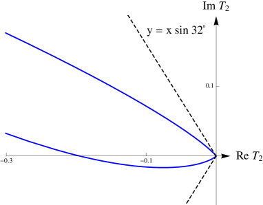
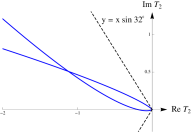
Figure 6. The functions $T_{2}^{\pm}$ in the complex plane.

Hence the angle of $T_{2}$ to the imaginary axis is at least $30^{\circ}$, and thus

$$\operatorname{Re}T_{2}\leq\frac{|b|}{8}\>\operatorname{Re}T_{2}^{\pm}\>.$$

Moreover, an explicit analysis (see the right of Figure 7) shows that

Figure 7. Lower bounds for $\operatorname{Re}T_{2}^{\pm}$.

$$\operatorname{Re}T_{2}^{\pm}\leq\left\{\begin{array}[]{cl}-u^{3}/10&\text{if~{}$0\leq u\leq 2$}\\[3.00003pt] -u^{2}/5&\text{if~{}$u>2$\>.}\end{array}\right.$$

We conclude that

$$\operatorname{Re}T_{2}\leq-\frac{|b|}{80}\times\left\{\begin{array}[]{cl}u^{3}&\text{if~{}$0\leq u\leq 2$}\\[3.00003pt] 2u^{2}&\text{if~{}$u>2$\>.}\end{array}\right.$$ (3.50)

To estimate $T_{3}$, we note that

$$T_{3}=\frac{|b|}{12}\>e^{i(-90+3\alpha_{\pm}+\Delta)}\>u^{3}=\frac{|b|}{12}\times\left\{\begin{array}[]{cl}e^{i(234^{\circ}+\Delta)}&\text{in case~{}$+$}\\ e^{i(120^{\circ}+\Delta)}&\text{in case~{}$-$\>.}\end{array}\right.$$

Thus $T_{3}$ lies in the left half plane, and its angle with the imaginary axis is at least $28^{\circ}$. Hence

$$\operatorname{Re}T_{3}\leq-\sin 28^{\circ}\>|T_{3}|\leq-\frac{|b|}{50}\>u^{3}\>.$$ (3.51)

Using (3.49), (3.50) and (3.51) in (3.44), we conclude that

$$\operatorname{Re}\big{(}f(t)-f(t_{0})\big{)} \leq-\frac{1}{200}\left|8d+b\right|u^{2}-\frac{|b|}{80}\times\left\{\begin{array}[]{cl}u^{3}&\text{if~{}$0\leq u\leq 2$}\\[3.00003pt] 2u^{2}&\text{if~{}$u>2$\>.}\end{array}\right.$$ (3.54)

$$\operatorname{Re}\big{(}\tilde{f}(t)-f(t_{0})\big{)} \leq-\frac{1}{200}\left|8d+b\right|u^{2}-\frac{|b|}{50}\>u^{3}$$ (3.55)

As the estimate (3.40) also holds in the case when $t_{0}^{2}\approx b/4$, we do not want to make use of the first summands in (3.54) and (3.55). For simplicity, we drop them,

$$\operatorname{Re}\big{(}f(t)-f(t_{0})\big{)} \leq-\frac{|b|}{80}\times\left\{\begin{array}[]{cl}u^{3}&\text{if~{}$0\leq u\leq 2$}\\[3.00003pt] 2u^{2}&\text{if~{}$u>2$\>.}\end{array}\right.$$

$$\operatorname{Re}\big{(}\tilde{f}(t)-f(t_{0})\big{)} \leq-\frac{|b|}{50}\>u^{3}.$$

Then

$$\int_{L}^{\infty}e^{\operatorname{Re}\big{(}\tilde{f}(t)-f(t_{0})\big{)}}\>du \leq\int_{L}^{\infty}e^{-\frac{|b|}{100}\>u^{3}}\>du\leq e^{-\frac{|b|\>L^{3}}{200}}\int_{0}^{\infty}e^{-\frac{|b|}{200}\>u^{3}}\>du$$

$$=e^{-\frac{|b|\,L^{3}}{200}}\>\Gamma\Big{(}\frac{4}{3}\Big{)}\>\left(\frac{200}{|b|}\right)^{\frac{1}{3}}\leq 6\>|b|^{-\frac{1}{3}}\>e^{-\frac{|b|\,L^{3}}{200}}$$

$$\int_{L}^{\infty}e^{\operatorname{Re}\big{(}\tilde{f}(t)-f(t_{0})\big{)}}\>du \leq\int_{L}^{\infty}\left(e^{-\frac{|b|}{80}\>u^{3}}+e^{-\frac{|b|}{40}\>u^{2}}\right)\>du$$

$$\leq 6\>|b|^{-\frac{1}{3}}\>e^{-\frac{|b|\,L^{3}}{200}}+e^{-\frac{|b|\,L^{2}}{80}}\int_{0}^{\infty}e^{-\frac{|b|\,L^{2}}{80}}\>du$$

$$\leq 6\>|b|^{-\frac{1}{3}}\>e^{-\frac{|b|\,L^{3}}{200}}+8\>|b|^{-\frac{1}{2}}\>e^{-\frac{|b|\,L^{2}}{80}}\>.$$

On the interval $[0,L]$, we can again follow the argument in (3.25) to obtain

$$\Big{|}e^{f(t)-f(t_{0})}-e^{\tilde{f}(t)-f(t_{0})}\Big{|}\leq|f(t)-\tilde{f}(t)|\>.$$

Using that $\tilde{f}$ is the cubic Taylor approximation to $f$, we obtain similar to (3.26) that

$$|f(t)-\tilde{f}(t)|\leq\frac{|\tau|^{4}}{4!}\>\frac{3\,|b|}{2}\sup_{\tau}\frac{1}{|1+\tau|^{4}}\leq|b|\,u^{4}\>.$$

Here in the last step we used that, according to (3.42), on the contour $\Gamma$ the inequality $|1+\tau|\geq 1/2$ holds. As a consequence,

$$\int_{0}^{L}\Big{|}e^{f(t)-f(t_{0})}-e^{\tilde{f}(t)-f(t_{0})}\Big{|}du\leq\frac{|b|}{5}\,L^{5}\>.$$ (3.56)

Adding up all error terms, in view of (3.43) we obtain for any $L>0$ the inequality

$$\left|U_{a}^{-}(z)-\tilde{U}_{a}(z)\right| \leq 2\,e^{-\frac{\operatorname{Re}z^{2}}{4}+f(t_{0})}\>|t_{0}|\left(\frac{|b|}{5}\,L^{5}+12\>|b|^{-\frac{1}{3}}\>e^{-\frac{|b|\,L^{3}}{200}}+8\>|b|^{-\frac{1}{2}}\>e^{-\frac{|b|\,L^{2}}{80}}\right)$$

Choosing

$$L=\frac{200}{|b|}\>\log\big{(}1+|b|^{\frac{1}{3}}\big{)},$$

we obtain the estimate

$$\frac{e^{\frac{\operatorname{Re}z^{2}}{4}-f(t_{0})}}{|t_{0}|}\left|U_{a}^{-}(z)-\tilde{U}_{a}(z)\right| \leq 1600\cdot 5^{\frac{1}{3}}\>|b|^{-\frac{2}{3}}\>\log^{\frac{5}{3}}\big{(}1+|b|^{\frac{1}{3}}\big{)}+24\,|b|^{-\frac{2}{3}}$$

$$\qquad+16\,|b|^{-\frac{1}{2}}\>\exp\Big{(}-\frac{1}{4}\>5^{\frac{1}{3}}\>|b|^{\frac{1}{3}}\>\log^{\frac{2}{3}}\big{(}1+|b|^{\frac{1}{3}}\big{)}\Big{)}$$

$$\leq 40\>|b|^{-\frac{2}{3}}\left(1+100\,\log^{\frac{5}{3}}\big{(}1+|b|^{\frac{1}{3}}\big{)}\right).$$

This proves (3.40).

The estimate (3.41) also applies in the case when $|b|$ is small. This motivates us to drop the last summands in (3.54) and (3.55),

$$\operatorname{Re}\big{(}f(t)-f(t_{0})\big{)},\operatorname{Re}\big{(}\tilde{f}(t)-f(t_{0})\big{)}\leq-\frac{1}{200}\left|8d+b\right|u^{2}\>.$$

Then

$$\int_{L}^{\infty} e^{\operatorname{Re}\big{(}f(t)-f(t_{0})\big{)}}\,du\leq\int_{L}^{\infty}e^{-\frac{|8d+b|}{200}\>u^{2}}du$$

$$\leq e^{-\frac{|8d+b|}{400}\,L^{2}}\int_{0}^{\infty}e^{-\frac{|8d+b|}{400}\,u^{2}}du=\sqrt{2\pi}\>5\,|8d+b|^{-\frac{1}{2}}\>e^{-\frac{|8d+b|}{400}\,L^{2}}\>,$$

and similarly for $\tilde{f}$. The integral over $[0,L]$ can be estimated again by (3.56). We thus obtain

$$\left|U_{a}^{-}(z)-\tilde{U}_{a}(z)\right|\leq 2\,e^{-\frac{\operatorname{Re}z^{2}}{4}+f(t_{0})}\>|t_{0}|\left(\sqrt{2\pi}\>10\,|8d+b|^{-\frac{1}{2}}\>e^{-\frac{|8d+b|}{400}\,L^{2}}+\frac{|b|}{5}\,L^{5}\right).$$

Choosing

$$L=20\,|8d+b|^{-\frac{1}{2}}\>\log^{\frac{1}{2}}\Big{(}1+\frac{|8d+b|^{2}}{|b|}\Big{)}\>,$$

a short calculation gives (3.41).

Acknowledgments: We would like to thank Martin Muldoon for several helpful remarks and for introducing us to the literature of special functions. We are grateful to the Vielberth Foundation, Regensburg, for generous support.

References

[1]
S. Chandrasekhar, The Mathematical Theory of Black Holes, Oxford
Classic Texts in the Physical Sciences, The Clarendon Press Oxford University
Press, New York, 1998.
[2]
F. Finster and H. Schmid, Spectral estimates and non-selfadjoint
perturbations of spheroidal wave operators, J. Reine Angew. Math.
601 (2006), 71–107.
[3]
F. Finster and J. Smoller, Error estimates for approximate solutions of
the Riccati equation with real or complex potentials, arXiv:0807.4406
[math-ph], Arch. Ration. Mech. Anal. 197 (2010), no. 3, 985–1009.
[4]
by same author, Error estimates for approximate solutions of the angular
Teukolsky equation in the Kerr geometry, in preparation (2013).
[5]
by same author, A spectral representation for spin-weighted spheroidal wave
operators with complex aspherical parameter, in preparation (2013).
[6]
L. Hörmander, The Analysis of Linear Partial Differential
Operators. I, second ed., Grundlehren der Mathematischen Wissenschaften
[Fundamental Principles of Mathematical Sciences], vol. 256, Springer-Verlag,
Berlin, 1990, Distribution theory and Fourier analysis.
[7]
F.W.J. Olver, Asymptotics and Special Functions, Academic Press [A
subsidiary of Harcourt Brace Jovanovich, Publishers], New York-London, 1974.
[8]
F.W.J. Olver, D.W. Lozier, R.F. Boisvert, and C.W. Clark (eds.), Digital
Library of Mathematical Functions, National Institute of Standards and
Technology from http://dlmf.nist.gov/ (release date 2011-07-01), Washington,
DC, 2010.
[9]
N.M. Temme and R. Vidunas, Parabolic cylinder functions: Examples of
error bounds for asymptotic expansions, arXiv:math/0205045v1 [math.CA],
Anal. Appl. (Singap.) 1 (2003), no. 3, 265–288.
[10]
S.A. Teukolsky, Perturbations of a rotating black hole I. Fundamental
equations for gravitational, electromagnetic, and neutrino-field
perturbations, Astrophys. J. 185 (1973), 635–647.