Hosotani mechanism in higher dimensional Lee-Wick theory

Abstract

Hosotani mechanism in higher-dimensional Lee-Wick theory is investigated. The symmetry breaking mechanism proposed by Hosotani is studied at one-loop level through a toy model in this theory. We find that the phase diagram of symmetry and masses of fields are modified from the original one if masses of Lee-Wick particles are in the same order of the inverse of the compactification scale.

I Introduction

Lee-Wick theory has been proposed as a candidate of finite theory for QED LW . In the theory, a massive ghost field is introduced and is expected to work as in the manner of Pauli-Villars regularization scheme. Although the existence of such a ghost field seems to be problematic for some authors prob , possible interpretations have been suggested, for example, instability of the massive particle LW ; GOW .

In spite of of the suspicion on its consistency, Lee-Wick theory has been applied to not only the standard model and unification GOW ; LWSM but also to cosmology of the bouncing universe bounce . In these days, various physical consequences have been studied eagerly, even in still higher derivative models hd , while some open questions in their basic concept is left unresolved.

In particle physics, it is interesting to apply Lee-Wick theory to solve the hierarchy problem. If the mass of the ghost particles are larger than TeV scale, some quadratic divergences and other relic effects become invisible. Such a model does not need supersymmetry, and we are ready to study the scenario à la Lee-Wick in the analysis of high-energy experiments.

In Lee-Wick unified models, however, the origin of the Higgs boson and/or the structure of symmetry breaking sector are still unexplained. In this reason, we come to consider so-called gauge-Higgs unification, or the higher-dimensional origin of the Higgs field Hosotani ; Toms ; GH in the context of Lee-Wick theory. In the present paper, a simple toy model with an $SU(2)$ gauge symmetry is examined. In the model, we take a circle as an extra dimension. For a phenomenologically viable models, we should use orbifolds for extra dimensions to obtain chiral fermions and consider selected boundary conditions on gauge and fermionic fields GH . Nevertheless, we will show some remarkable features about symmetry breaking, which may be worth applying to the phenomenological study in future work.

Another reason to examine the gauge-Higgs unified scheme is in the interest on the quantum effect. The tree-level mass of the scalar degree of freedom, which comes from an extra component of the gauge field, is protected from quantum corrections because of the gauge symmetry in the higher-dimensional theory. Then, the quantum effective potential governs the symmetry breakdown. Whereas in Lee-Wick theory, the one-loop contribution of the ghost fields modifies the effective potential in the theory as well as its divergent behavior. We expect new varieties of symmetry breaking patterns in Lee-Wick gauge-Higgs unified models.

In this paper, we consider the higher dimensional model of Lee-Wick theory and the one-loop effect on the symmetry breaking mechanism proposed by Hosotani. In Sec. II, we review the Lee-Wick gauge theory and its extension to higher dimensional theory. Then, we incorporate Hosotani mechanism into the five dimensional Lee-Wick theory and investigate mass levels of the particles obtained by compactification on $R^{4}\times S^{1}$. In Sec. III, we calculate the one-loop effective potential and study the symmetry breaking in our model. We discuss the mass of the vector and scalar bosons in our model in Sec. IV. Finally, Sec. V is devoted to discussion.

II The higher derivative gauge theory in five dimensions

The Lagrangian density for the Lee-Wick non-Abelian gauge theory is given by GOW

$${\cal L}=-\frac{1}{2}{\rm tr~{}}\hat{F}^{\mu\nu}\hat{F}_{\mu\nu}+\frac{1}{M_{A}^{2}}{\rm tr~{}}\hat{D}_{\mu}\hat{F}^{\mu\nu}\hat{D}^{\lambda}\hat{F}_{\lambda\nu}\,,$$ (1)

where $\hat{F}_{\mu\nu}\equiv\partial_{\mu}\hat{A}_{\nu}-\partial_{\nu}\hat{A}_{\mu}-ig[\hat{A}_{\mu},\hat{A}_{\nu}]$ and $g$ is the gauge coupling. By using auxiliary field $\tilde{A}_{\nu}$, the Lagrangian (1) is rewritten as

$${\cal L}=-\frac{1}{2}{\rm tr~{}}\hat{F}^{\mu\nu}\hat{F}_{\mu\nu}-2{\rm tr~{}}\tilde{A}_{\nu}\hat{D}_{\mu}\hat{F}^{\mu\nu}-{M_{A}^{2}}\,{\rm tr~{}}\tilde{A}^{\nu}\tilde{A}_{\nu}\,.$$ (2)

In this Lagrangian, the kinetic term of the fields does not take a diagonal form. If we define a linear combination of the fields $A_{\mu}\equiv\hat{A}_{\mu}-\tilde{A}_{\mu}$, we obtain the diagonalized Lagrangian GOW

$${\cal L} = -\frac{1}{2}{\rm tr~{}}{F}^{\mu\nu}{F}_{\mu\nu}+\frac{1}{2}{\rm tr~{}}(D^{\mu}\tilde{A}^{\nu}-D^{\nu}\tilde{A}^{\mu})(D_{\mu}\tilde{A}_{\nu}-D_{\nu}\tilde{A}_{\mu})-{M_{A}^{2}}\,{\rm tr~{}}\tilde{A}^{\nu}\tilde{A}_{\nu}$$ (3)

$$-ig{\rm tr~{}}([\tilde{A}_{\mu},\tilde{A}_{\mu}]F^{\mu\nu})+\cdots\,,$$

where ${F}_{\mu\nu}\equiv\partial_{\mu}{A}_{\nu}-\partial_{\nu}{A}_{\mu}-ig[{A}_{\mu},{A}_{\nu}]$ and $D_{\mu}\tilde{A}_{\nu}\equiv\partial_{\mu}\tilde{A}_{\nu}-ig[{A}_{\mu},\tilde{A}_{\nu}]$. Here, we omitted the irrelevant interaction terms for our purpose. The Lagrangian shows that the theory describes usual massless gauge bosons and vector ‘ghost’ bosons with mass $M_{A}$.

The Lee-Wick gauge theory in higher dimensions can be defined by the same Lagrangian density. Let us assume the five dimensional theory. Suppose that the spacetime topology is $R^{4}\times S^{1}$ where $R^{4}$ is a four dimensional spacetime and $S^{1}$ is a circle whose circumference is $L$. The five dimensional coordinates are represented by $(x^{i},y)=(x^{0},x^{1},x^{2},x^{3},y)$, where $0\leq y<L$. Now, the fifth component of the gauge field $A_{5}$ becomes scalar degrees of freedom in four dimensions.

Let us consider $SU(2)$ gauge theory in this spacetime, as a simple case. Then, the matrix-valued gauge field can be expressed by three component fields as $A_{\mu}=A_{\mu}^{a}\frac{\tau^{a}}{2}$, where $\tau^{a}$ is the $2\times 2$ Pauli matrix and $a=1,2,3$. Boundary conditions on $A_{\mu}$ is chosen definitely as follows:

$$A_{\mu}(x,y+L)=A_{\mu}(x,y)\,.$$ (4)

A constant vacuum gauge field is allowed on the multiply-connected space; the vacuum expectation value of the gauge field configuration plays the role of an ‘order parameter’. Hosotani and Toms have considered a simple model to show that one-loop vacuum effect determines the order parameter Hosotani ; Toms .

On the circle $S^{1}$ as an extra dimension, non zero vacuum gauge configuration is permitted. In our case, we set

$$gLA_{5}=\frac{1}{2}\left[\begin{array}[]{cc}\phi&0\\ 0&-\phi\end{array}\right]=\frac{\phi}{2}\tau_{3}\,,$$ (5)

where the vacuum gauge field has been diagonalized by using the freedom of gauge transformations. Therefore, roughly speaking, the extra-dimensional component of the gauge field behaves as the Higgs field in the adjoint representation. We should notice that $gLA_{5}$ is equivalent to $gLA_{5}+2\pi\ell\tau_{3}$ ($\ell$: integer) under non-singular gauge transformations. Thus, we can only restrict $0\leq\phi<4\pi$ by gauge transformations.

In the five dimensional Lee-Wick gauge theory, in view of the four dimensional flat space, we find that the propagator has ladders of poles at

$$p^{2}=\frac{1}{L^{2}}(2\pi\ell+\phi)^{2}\equiv m_{1}^{2}(\ell)\equiv m_{2}^{2}(\ell)\qquad(\ell{\rm:~{}integer})$$ (6)

which are for the four-dimensional descendant fields of $A^{1}_{i}$ and $A^{2}_{i}$, where $i=0,1,2,3$,

$$p^{2}=\frac{1}{L^{2}}(2\pi\ell)^{2}\equiv m_{3}^{2}(\ell)\qquad(\ell{\rm:~{}integer})$$ (7)

which are for the descendant fields of $A^{3}_{i}$. Here, $p^{2}$ denotes the four dimensional momentum squared, of course. Note that the fields $A_{5}^{1}$ and $A_{5}^{2}$ are absorbed by $A_{i}^{1}$ and $A_{i}^{2}$ and become the longitudinal components of the massive vector fields in general.

On the other hand, the Lee-Wick ghost field has poles at

$$p^{2}=\frac{1}{L^{2}}(2\pi\ell+\phi)^{2}+M_{A}^{2}\equiv\tilde{m}_{1}^{2}(\ell)\equiv\tilde{m}_{2}^{2}(\ell)\qquad(\ell{\rm:~{}integer})$$ (8)

which are for the four-dimensional descendant fields of $\tilde{A}^{1}_{\mu}$ and $\tilde{A}^{2}_{\mu}$,

$$p^{2}=\frac{1}{L^{2}}(2\pi\ell)^{2}+M^{2}_{A}\equiv\tilde{m}_{3}^{2}(\ell)\qquad(\ell{\rm:~{}integer})$$ (9)

which are for the descendant fields of $\tilde{A}^{3}_{\mu}$. Note that $\tilde{m}^{2}_{a}=m^{2}_{a}+M_{A}^{2}$. In the view of four dimensional spacetime, $\tilde{A}_{\mu}$ is decomposed to massive vector and scalar fields.

In general, non zero $\phi$ shifts the mass level; this effect reduces the number of the massless fields in four dimensions within the Kaluza-Klein point of view. We will see how the value of $\phi$ is determined by the one-loop quantum effect in the next section.

III One-Loop Quantum Effect and symmetry breaking

To calculate the one-loop effective potential, we use integration of the Euclidean momenta. The choice of calculation is subtle in the higher-derivative theory. According to Ref. AG , the Euclidean approach naturally leads to the cancellation of the leading divergence in the loop effect, as is suitable for the motivation of Lee-Wick theory.

The one-loop vacuum energy density from the $SU(2)$ gauge and Lee-Wick fields discussed in the previous section is given by

$$V_{A}=\sum_{a=1}^{3}\sum_{\ell=-\infty}^{\infty}\int\frac{d^{4}k_{E}}{(2\pi)^{4}}\left\{\frac{3}{2}\ln[k_{E}^{2}+m_{a}^{2}(\ell)]-2\ln[k_{E}^{2}+\tilde{m}_{a}^{2}(\ell)]\right\}\,.$$ (10)

Incidentally, the relative sign appearing in this expression agrees with the result for thermal free energy considered in Ref. thermo , provided that we use the Matsubara formalism.

Here, we shall briefly show the calculation of the potential treated in the text. In the space $R^{d}\times S^{1}$, the effective potential is formally expressed by the Schwinger proper-time integral Schwinger . Thus, we find

$$V_{A}=-\frac{1}{2(4\pi)^{2}}\int^{\infty}_{\Lambda^{-2}}\frac{dt}{t^{3}}\,K(t)(3-4e^{-M_{A}^{2}t})\,,$$ (11)

where the kernel function is defined as

$$K(t)=\sum_{a}\sum_{\ell}\exp[-m^{2}_{a}(\ell)t]\,,$$ (12)

and $\Lambda$ is the UV cut-off scale.

To evaluate the kernel function $K(t)$, we can use the inversion relation

$$\sum_{\ell=-\infty}^{\infty}\exp\left[-\left(\frac{2\pi}{L}\right)^{2}(\ell-\chi)^{2}\,t\right]=\frac{L}{\sqrt{4\pi\,t}}\sum_{\ell=-\infty}^{\infty}\exp\left(-\frac{L^{2}\ell^{2}}{4t}\right)\cos(2\pi\ell\chi)\,.$$ (13)

Using this formula, we can see that the UV divergent part comes from the contribution of $\ell=0$ in the sum on the right-hand side of the expression and it is independent of $\phi$. Thus, we obtain a finite one-loop effective potential for $\Lambda\rightarrow\infty$ by discarding the divergent constant. Then, the integration over the proper-time can be carried out by the help of an integral representation of the modified Bessel function of the second kind Takenaga

$$\int_{0}^{\infty}\frac{dt}{t^{\nu+1}}\exp\left(-\frac{L^{2}\ell^{2}}{4t}-M^{2}t\right)=2\left(\frac{2M}{L\ell}\right)^{\nu}K_{\nu}(ML\ell)\,.$$ (14)

Further, an explicit form of $K_{5/2}(z)$

$$K_{5/2}(z)=\sqrt{\frac{\pi}{2z}}\left(1+\frac{3}{z}+\frac{3}{z^{2}}\right)e^{-z}\,$$ (15)

leads to the following expression:

$$V_{A}=-\frac{9}{4\pi^{2}L^{4}}\sum_{\ell=1}^{\infty}\frac{w_{A}(M_{A}L\ell)}{\ell^{5}}[2\cos(\ell\phi)+1]\,,$$ (16)

where the weight factor $w_{A}(x)$ is defined as

$$w_{A}(x)=1-\frac{4}{3}e^{-x}\left(1+x+\frac{1}{3}x^{2}\right)\,.$$ (17)

We can see that $w_{A}(x)$ becomes negative for $x<1.41$. Thus, the shape of the effective potential can become ‘reversed’ if $M_{A}L$ takes a small value, and then the symmetry breaking such that $\langle\phi\rangle\neq 0$ occurs. Unfortunately, because the study on a Lee-Wick model in four dimensions GOW suggests $M_{A}>1$TeV, the mass of the vector bosons should be very large in this case.

In order to naturally realize the symmetry breaking vacuum, we can add fermionic fields into the theory. Now, the Lee-Wick Dirac fermion is introduced, which is governed by the Lagrangian

$${\cal L}_{\psi}=-i\bar{\psi}^{a}{D\!\!\!\!/}\left(1+\frac{{D\!\!\!\!/}{D\!\!\!\!/}}{M_{\psi}^{2}}\right)\psi^{a}\,,$$ (18)

where ${D\!\!\!\!/}=\gamma^{\mu}D_{\mu}$ GOW ; HK . If the spacetime is flat with an infinite extension and gauge fields vanish, the pole of the propagator of the Dirac field is located at $p^{2}=0$ and $p^{2}=M_{\psi}^{2}$, and the latter is a ghost pole.

As for the case of the Kaluza-Klein background spacetime, i.e., where an extra dimension is compactified on $S^{1}$ with the radius $L/(2\pi)$, we obtain the ladder of poles for four dimensional fields. We consider the $SU(2)$ adjoint fermion $\psi^{a}$ $(a=1,2,3)$. Further, we assume a periodic boundary condition in the extra dimension as

$$\psi^{a}(x,y+L)=\psi^{a}(x,y)\,.$$ (19)

for simplicity. Then, the same degrees of freedom with the same poles as the Yang-Mills field can be found in the fermionic field, except for the replacement $M_{A}\rightarrow M_{\psi}$. Thus, we can find that the contribution of the one-loop quantum effects of fermionic fields becomes

$$V_{\psi}=N_{\psi}\frac{3}{\pi^{2}L^{4}}\sum_{\ell=1}^{\infty}\frac{w_{\psi}(M_{\psi}L\ell)}{\ell^{5}}[2\cos(\ell\phi)+1]\,,$$ (20)

where $N_{\psi}$ is the number of the fermion fields which belong to the adjoint representation of $SU(2)$. The weight factor $w_{\psi}(x)$ is defined as

$$w_{\psi}(x)=1-e^{-x}\left(1+x+\frac{1}{3}x^{2}\right)\,.$$ (21)

Note that $w_{\psi}(x)\rightarrow 1$ for $x\rightarrow\infty$ and $w_{\psi}(x)\rightarrow\frac{1}{6}x^{2}+O(x^{4})$ for $x\rightarrow 0$.

Therefore, the total effective potential for the system under consideration is given by

$$V_{eff}(\phi)=-\frac{3}{4\pi^{2}L^{4}}\sum_{\ell=1}^{\infty}\frac{3w_{A}(M_{A}L\ell)-4N_{\psi}w_{\psi}(M_{\psi}L\ell)}{\ell^{5}}[2\cos(\ell\phi)+1]\,.$$ (22)

The emergence of symmetry breaking is indicated by instability of the symmetric vacuum, or

$$V^{\prime\prime}_{eff}(0)=\frac{3}{2\pi^{2}L^{4}}\sum_{\ell=1}^{\infty}\frac{3w_{A}(M_{A}L\ell)-4N_{\psi}w_{\psi}(M_{\psi}L\ell)}{\ell^{3}}<0\,.$$ (23)

The symmetry broken phase is indicated in Fig. 1 in the parameter space spanned by $M_{A}L$ and $M_{\psi}L$.

Figure 1: Phase structure of the model. The solid line indicates the boundary of the two phases for $N_{\psi}=1$, the broken line indicates that for $N_{\psi}=2$, and the dotted line indicates that for $N_{\psi}=3$.

In the region above the line, the gauge symmetry is broken. For a sufficiently large $M_{\psi}L$, the $SU(2)$ symmetry is broken for any value for $M_{A}L$. Conversely speaking, for a sufficiently large $M_{A}L$, there is a lower bound value of $M_{\psi}L$ for symmetry breaking, which is nearly constant. For $N_{\psi}=1$, the symmetry breaking occurs if $M_{\psi}L\geq 3.4$.

IV Mass of the vector and scalar bosons

The phase diagrams are very similar for the different numbers of the fermions, $N_{\psi}(\geq 1)$. Thus, from here, we consider only the case of $N_{\psi}=1$ in our model.

In our toy model, the order parameter takes the ‘topological’ value $\langle\phi\rangle=\pi$ or $\langle\phi\rangle=0$ in the almost region of the parameter space. We find, however, the order parameter $\langle\phi\rangle$ takes the value $0<\langle\phi\rangle<\pi$ for the narrow region of the parameter space. This region is shown in Fig. 2 as the narrow region between two lines.

Figure 2: The value of the order parameter $\langle\phi\rangle$. In the narrow parameter region between two solid lines, $\langle\phi\rangle$ takes $0<\langle\phi\rangle<\pi$.

Because the boundaries are almost parallel to the $M_{A}L$ axis for a large $M_{A}L$, we consider the case with $M_{A}L\rightarrow\infty$ hereafter.

We define the normalized potential $v(\phi)$ as $V_{eff}(\phi)=\frac{3}{2\pi^{2}L^{4}}v(\phi)+$(independent of $\phi$). Namely, the normalized potential is written by

$$v(\phi)=-\sum_{\ell=1}^{\infty}\frac{3w_{A}(M_{A}L\ell)-4w_{\psi}(M_{\psi}L\ell)}{\ell^{5}}\cos\ell\phi\,.$$ (24)

The shape of the potential $v(\phi)$ (shown in the region $0\leq\phi\leq 2\pi$) is sensitive against the variation of $M_{\psi}L$ in the range from $3.2$ to $3.8$, as seen from Fig. 3.

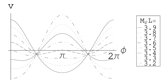
Figure 3: The profiles of the normalized potential $v(\phi)$ for $M_{A}L\rightarrow\infty$ and various values of $M_{\psi}L$, as indicated in the legend.

As seen from the graph of the potential, the infinite sum in the expression of the potential can be well approximated by taking the first two terms in this parameter region. Thus, the approximate potential is

$$v_{app}(\phi) = \left\{1-4e^{-M_{\psi}L}\left[1+M_{\psi}L+\frac{(M_{\psi}L)^{2}}{3}\right]\right\}\cos\phi$$ (25)

$$+\frac{1}{2^{5}}\left\{1-4e^{-2M_{\psi}L}\left[1+2M_{\psi}L+\frac{4(M_{\psi}L)^{2}}{3}\right]\right\}\cos 2\phi\,.$$

Figure 4: The vacuum expectation value of $\phi$ against $M_{\psi}L$.

Using this approximation, we find the value of the order parameter $\langle\phi\rangle$ and exhibited in Fig. 4. We remember that two vector bosons acquire mass of $m=\langle\phi\rangle/L$ and one of the gauge bosons remain massless, as lowest masses of the Kaluza-Klein spectra. The lowest masses of the adjoint fermions are similar to the vector bosons.

One light scalar degree of freedom is left in any phases. This is a scalar field which comes from the extra component of the gauge field, that is, $\sqrt{L}A_{5}^{a=3}$. The scalar is classically massless, however, as seen so far, the one-loop quantum effect causes its mass. The mass of this boson is obtained from the second derivative of the effective potential and we find

$$m^{2}_{S}=\frac{3g^{2}}{2\pi^{2}L^{3}}v^{\prime\prime}(\langle\phi\rangle)\,.$$ (26)

Note that the dimensionless four dimensional gauge coupling is $g/\sqrt{L}$ in our model.

The mass of the scalar boson plotted against $M_{\psi}L$ is shown in Fig. 5.

Figure 5: Mass of the scalar boson.

We find that the mass of the scalar boson is always smaller than the mass of the vector bosons in the symmetry-broken phase, as long as the four dimensional gauge coupling takes a moderate value $(g/\sqrt{L}<1)$.

V Discussion

In this paper, we have calculated the one-loop effective potential for the simple model of five dimensional Lee-Wick gauge theory with adjoint fermions and have investigated its phase space of the symmetry. It turns out that the mass of the Lee-Wick particle has much influence on the symmetry breaking through the effective potential. We have also found that the smaller mass scales than the compactification scale $1/L$ can appear if the Lee-Wick fermion mass scale is in a certain narrow parameter region.

To study a realistic gauge-Higgs unification scenario, we should incorporate non-trivial geometry such as orbifolds and Randall-Sundrum type warped space. Our toy model, however, has shown the effect of masses of Lee-Wick particles qualitatively.

In future work, we should examine more elaborated models mentioned above, their finite temperature behavior (which is interesting as four dimensional models in Ref. thermo ), and higher-loop quantum effect and non-perturbative effect on the models. We also wish to study the flux in the extra space in the Lee-Wick model. In the related thoughts, the possible modification of Nielsen-Olesen instability NO in the Lee-Wick Yang-Mills theory will also be studied with much interest.

References

- (1) T. D. Lee and G. C. Wick, Nucl. Phys. B9 (1969) 209; Phys. Rev. D2 (1970) 1033; Phys. Rev. D3 (1971) 1046. R. E. Cutkosky, P. V. Landshoff, D. I. Olive and J. C. Polkinghorne, Nucl. Phys. B12 (1969) 281.
- (2) N. Nakanishi, Phys. Rev. D3 (1971) 81; Phys. Rev. D3 (1971) 1343. D. G. Boulware and D. J. Gross, Nucl. Phys. B233 (1984) 1.
- (3) B. Grinstein, D. O’Connell and M. B. Wise, Phys. Rev. D77 (2008) 025012.
- (4) T. G. Rizzo, JHEP 0706 (2007) 070. J. R. Espinosa, B. Grinstein, D. O’Connell and M. B. Wise Phys. Rev. D77 (2008) 085002. T. R. Dulaney and M. B. Wise Phys. Lett. B658 (2008) 230. F. Krauss, T. E. J. Underwood and R. Zwicky, Phys. Rev. D77 (2008) 015012; Erratum-ibid. D83 (2011) 019902. B. Grinstein, D. O’Connell and M. B. Wise, Phys. Rev. D77 (2008) 065010. T. G. Rizzo, JHEP 0801 (2008) 042. B. Grinstein and D. O’Connell, Phys. Rev. D78 (2008) 105005. E. Alvarez, L. Da Rold, C. Schat and A. Szynkman, JHEP 0804 (2008) 026. T. E. J. Underwood and R. Zwicky, Phys. Rev. D79 (2009) 035016. C. D. Carone and R. F. Lebed, Phys. Lett. B668 (2008) 221. C. D. Carone and R. Primulando, Phys. Rev. D80 (2009) 055020. E. Alvarez, L. Da Rold, C. Schat and A. Szynkman, JHEP 0910 (2009) 023. M. B. Wise, Int. J. Mod. Phys. A25 (2010) 587. R. Sekhar Chivukula, A. Farzinnia, R. Foadi and E. H. Simmons, Phys. Rev. D81 (2010) 095015. E. Alvarez, E. C. Leskow and J. Zurita, Phys. Rev. D83 (2011) 115024. T. Figy and R. Zwicky, JHEP 1110 (2011) 145.
- (5) Y.-F. Cai, T. Qiu, R. Brandenberger and X. Zhang, Phys. Rev. D80 (2009) 023511. J. Karouby and R. Brandenberger, Phys. Rev. D82 (2010) 063532. J. Karouby, T. Qiu and R. Brandenberger, Phys. Rev. D84 (2011) 043505. I. Cho and O-K. Kwon, JCAP 1111 (2011) 043.
- (6) C. D. Carone and R. F. Lebed, JHEP 0901 (2009) 043. C. D. Carone, Phys. Lett. B677 (2009) 306. R. F. Lebed and R. H. TerBeek, arXiv:1205.3213 [hep-ph].
- (7) Y. Hosotani, Phys. Lett. B126 (1983) 309.
- (8) D. Toms, Phys. Lett. B126 (1983) 445.
- (9) Y. Kawamura, Prog. Theor. Phys. 103 (2000) 613.
- (10) I. Antoniadis, E. Dudas and D. M. Ghilencea, JHEP 0803 (2008) 045. D. M. Ghilencea, Mod. Phys. Lett. A23 (2008) 711.
- (11) B. Fornal, B. Grinstein and M. B. Wise Phys. Lett. B674 (2009) 330. K. Bhattacharya and S. Das, Phys. Rev. D84 (2011) 045023; Phys. Rev. D86 (2012) 025009; arXiv:1208.0191 [hep-ph].
- (12) J. Schwinger, Phys. Rev. 82 (1951) 664.
- (13) K. Takenaga, Phys. Lett. B570 (2003) 244.
- (14) T. Hamazaki and T. Kugo, Prog. Theor. Phys. 92 (1994) 645.
- (15) P. de Forcrand, A. Kurkela and M. Panero JHEP 1006 (2010) 050.
- (16) N. K. Nielsen and P. Olesen, Nucl. Phys. B144 (1978) 376.