Wireless Scheduling with Dominant Interferers and Applications to Femtocellular Interference Cancellation

Abstract

We consider a general class of wireless scheduling and resource allocation problems where the received rate in each link is determined by the actions of the transmitter in that link along with a single dominant interferer. Such scenarios arise in a range of scenarios, particularly in emerging femto- and picocellular networks with strong, localized interference. For these networks, a utility maximizing scheduler based on loopy belief propagation is presented that enables computationally-efficient local processing and low communication overhead. Our main theoretical result shows that the fixed points of the method are provably globally optimal for arbitrary (potentially non-convex) rate and utility functions. The methodology thus provides globally optimal solutions to a large class of inter-cellular interference coordination problems including subband scheduling, dynamic orthogonalization and beamforming whenever the dominant interferer assumption is valid. The paper focuses on applications for systems with interference cancellation (IC) and suggests a new scheme on optimal rate control, as opposed to traditional power control. Simulations are presented in industry standard femtocellular network models demonstrate significant improvements in rates over simple reuse 1 without IC, and near optimal performance of loopy belief propagation for rate selection in only one or two iterations.

I Introduction

A central challenge in next-generation cellular networks is the presence of strong interference. This feature is particularly prominent in emerging femto- and pico-cellular networks where, due to ad hoc and unplanned deployments, restricted association and mobility in small cell geometries, mobiles may be exposed to much higher levels of interference than in traditional planned macrocellular networks [1, 2, 3]. Methods for advanced intercellular interference coordination (ICIC) have thus been a key focus of 3GPP LTE-Advanced standardization efforts [4] and other cellular standards organizations [5].

This work considers a class of general resource allocation and scheduling problems where the received rate in each link is determined primarily by the actions of the transmitter in that link along with a single dominant interferer. Interference in traditional macrocellular networks, of course, generally do not follow this assumption as there are typically a large number of mobiles per cell, and interference generally arises from an aggregate of signals from many sources in the network. However, in emerging small cell networks with higher cell densities, the number of mobiles per cell is significantly reduced and strong interference is most often due to the poor placement of the mobile relative to a single victim or interfering cell to which the mobile is not connected to.

For such dominant interference networks, we propose a novel ICIC algorithm based on graphical models and message passing. Graphical models [6, 7] are a widely-used tool for high-dimensional optimization and Bayesian inference problems applicable whenever the objective function or posterior distribution factors into terms with small numbers of variables. Methods such as loopy belief propagation (BP) then reduce the global problem to a sequence of smaller local problems associated with each factor. The outputs of the local problems are combined via message passing. The loopy BP methodology is particularly well-suited to wireless scheduling problems since the resulting algorithms are inherently distributed and require only local computations. Indeed, [8] showed that many widely-used network routing, congestion control and power control algorithms can be interpreted as instances of the sum-product variant of loopy BP. More recently, [9, 10] used BP techniques for networks with contention graphs, [11] proposed BP for MIMO systems, and [12, 13] considered a general class of ICIC problems with weak interference exploiting an approximate BP technique in [14].

For dominant interferer networks considered in this paper, we apply loopy BP methods to a general network utility maximization problem where the goal is to maximize a sum of utilities across a system with $n$ links. The utility in each link is assumed to be a function of a scheduling decision on the transmitter of that link, as well as the decision of at most one interfering link. Aside from this single dominant interferer assumption, the model is completely general, and can incorporate arbitrary channel relationships as well as sophisticated transmission schemes including subband scheduling, beamforming and dynamic orthogonalization – key features of advanced cellular technologies such as 3GPP LTE [15]. In addition, computing maximum weighted matching for queue stability [16] and maximization of sum utility of average rates for fairness [17] can be incorporated into this formulation.

We show that for single dominant interferer networks, loopy BP admits a particularly simple implementation: scheduling decisions can be computed with a small number of rounds of message passing, where each round involves simple local computations at the nodes along with communication only between the transmitter, receiver and dominant interferers in each link. Our simulations in commercial cellular models indicate near optimal performance in very small, sometimes only one or two, rounds – making the algorithms extremely attractive for practical implementations.

Moreover, we establish rigorously (Theorem 1) that any fixed point of the loopy BP algorithm is guaranteed to be globally optimal. Remarkably, this result relies solely on the dominant interferer assumption and otherwise applies to arbitrary utility functions and relationships between scheduling decisions on interfering and victim links. In particular, this optimality holds even for non-convex problems. Optimality results for loopy BP are generally difficult to establish: Aside from graphs that are cycle free, loopy BP generally only provides approximate solutions that may not be globally optimal. Our proof of global optimality in this case rests on showing that graphs with single dominant interferers have at most cycle in each connected component. The result then follows from a well-known optimality property in [18].

I-A Interference Cancelation and Rate Control

A target application of our methodology is for scheduling problems with interference cancelation (IC) [19, 20]. When an interfering signal is sufficiently strong, it can be decoded and canceled prior to or jointly with the decoding of the desired signal, thus eliminating the interference entirely. IC, particularly when used in conjunction with techniques such as rate splitting [21], is known to provide significant performance gains in scenarios with strong interference, where it may even be optimal or near optimal [22]. IC may also be useful for mitigating cross-tier interference between short-range (e.g. femtocellular) links operating below larger macrocells [23]. However, while improved computational resources have recently made IC implementable in practical receiver circuits [24, 25, 26], it is an open problem of how rates should be selected in larger networks when IC is available at the link-layer.

In this paper, we consider a network where the receiver in each link can jointly detect the desired signal along with at most one interfering link. The limitation of joint detection with at most one interfering link is reasonable since the likelihood of having two very strong interferers is low in most practical scenarios. The limit is also desirable since the computationally complexity at the receiver grows significantly with each additional link to perform joint detection with. For networks with IC, we propose to perform interference coordination based on rate control rather than traditional power control that has been the dominant method in cellular systems without IC [27]. Specifically, each transmitter operates at a fixed power, and the system utility is controlled by rate: increasing the rate improves the utility to the desired user, while decreasing the rate makes the transmission more “decodable” and hence “cancelable” at the receiver in any victim link. Hence, we suggest that in networks with IC, rate control, as opposed to power control, can be viable method for interference coordination.

II System Model

We consider a system with $n$ links, each link $i$ having one transmitter, TX$i$ and one receiver, RX$i$. In a cellular system, multiple logical links may be associated with the base station, either in the downlink or uplink. Each link $i$ is to make some scheduling decision, meaning a selection of some variable $x_{i}\in{\cal X}_{i}$ for some set ${\cal X}_{i}$. The scheduling decision could include choices, for example, of power, beamforming directions, rate or vectors of these quantities in the cases of multiple subbands – the model is general. Associated with each RX$i$ is a utility function representing some value or quality of service obtained by RX$i$. We assume that the utility function has the form

$$f_{i}(x_{i},x_{\sigma(i)}),$$

where $\sigma(i)\in\{1,\ldots,n\}$ is the index of one link other than $i$, representing the index of a dominant interferer to RX$i$. Thus, the assumption is that utility on each link $i$ is a function of the scheduling decisions of the serving transmitter, TX$i$, and one dominant interfering transmitter, TX$j$ for $j=\sigma(i)$. Generally, the dominant interferer with be the transmitter, other than the serving transmitter, with the lowest path loss to the receiver. The problem is to find the optimal solution

$$\widehat{\mathbf{x}}:=\mathop{\mathrm{arg\,max}}_{\mathbf{x}}F(\mathbf{x}),$$ (1)

where the objective function is the sum utility,

$$F(\mathbf{x}):=\sum_{i=1}^{n}f_{i}(x_{i},x_{\sigma(i)}).$$ (2)

The utility function $f(x_{i},x_{\sigma(i)})$ accounts for the link-layer conditions that determine the rates and along with quality-of-service (QoS) requirements for valuation of the traffic. A general treatment of utility functions for scheduling problems can be found in [28, 29]. The optimization problem (1) can be applied to both static and dynamic problems.

For static optimization, the scheduling vectors $x_{i}$ are selected once for a long time period and the utility function is typically of the form

$$f_{i}(x_{i},x_{\sigma(i)})=U_{i}(R_{i}(x_{i},x_{\sigma(i)})),$$ (3)

where $R_{i}(x_{i},x_{\sigma(i)})$ is the long-term rate as a function of the TX scheduling decision $x_{i}$ and decision $x_{\sigma(i)}$ on the dominant interferer, while $U_{i}(R)$ is the utility as a function of the rate. The problem formulation above can incorporate any of the common utility functions including: $U_{i}(R)=R$ which results in a sum rate optimization; $U_{i}(R)=\log(R)$ which is the proportional fair metric and $U_{i}(R)=-\beta R^{-\beta}$ for some $\beta>0$ called an $\beta$-fair utility. Penalties can also be added if there is a cost associated with the selection of the TX vector $x_{i}$ such as power.

To accommodate time-varying channels and traffic loads, many cellular systems enable fast dynamic scheduling in time slots in the order of 1 to 2 ms. For these systems, the utility maximization can be re-run in each time slot. One common approach is that in each time slot $t=0,1,2\ldots$, the scheduler uses a utility of the form

$$f_{i}(t,x_{i}(t),x_{\sigma(i)}(t))=w_{i}(t)R_{i}(t,(x_{i}(t),x_{\sigma(i)}(t)),\ \ \$$ (4)

where $w_{i}(t)$ is a time-varying weight given by the marginal utility

$$w_{i}(t)=\frac{\partial U_{i}(\overline{R}_{i}(t))}{\partial R},$$ (5)

and $\overline{R}_{i}(t)$ is exponentially weighted average rate updated as

$$\overline{R}_{i}(t+1)=(1-\alpha)\overline{R}_{i}(t)+\alpha R_{i}(t,\widehat{x}_{i}(t),\widehat{x}_{\sigma(i)}(t)),$$ (6)

where $\widehat{x}_{i}(t)$ and $\widehat{x}_{\sigma(i)}$ are the TX scheduling decisions on the serving and interfering links at time $t$. Any maxima of the optimization (1) with the weighted utility (4) is called a maximal weight matching. A well-known result of stochastic approximation [17] is that if $\alpha\rightarrow 0$, and the scheduler performs the maximum weight matching with the marginal utilities (5), then for a large class of processes, the resulting average rates will maximize the total utility $\sum_{i}U_{i}(\overline{R}_{i}(t))$.

The above utilities are designed for infinite backlog queues. For delay sensitive traffic, one can take the weights $w_{i}(t)$ to be the queue length or head-of-line delay. Maximal weight matching performed with these weights generally results in so-called throughput optimal performance [16]. These results also apply to multihop networks with the so-called backpressure weights.

II-A Systems with IC

As mentioned in the Introduction, a particularly valuable application of the methodology in this paper is for rate selection in systems with interference cancelation (IC). To simplify the exposition, we consider the following simple model of a system with IC: Assume the power of each transmitter, TX$j$, is fixed to some level $P_{j}$, and let $G_{ij}$ denote the gain from TX$j$ to RX$i$ as let $N_{i}$ denote the thermal noise at RX$i$. Without IC, the receiver RX$i$ would experience a signal-to-interference-and-noise ratio (SINR) given by

$$\rho_{i}:=\frac{G_{ii}P_{i}}{\sum_{k\neq i}G_{ik}P_{k}+N_{i}}.$$ (7)

If the interference is treated as Gaussian noise, and the system were to operate at the Shannon capacity, the set of rates $R_{i}$ attainable at RX$i$ would be limited to

$$R_{i}\leq\log_{2}(1+\rho_{i}).$$ (8)

We call this set of achievable rates the reuse 1 region, since this set is precisely the rates achievable in a cellular system operating with frequency reuse 1 (i.e. all transmitters transmitting across the entire bandwidth) and treating interference as noise. We denote the reuse 1 region by ${\mathcal{C}}_{\rm reuse1}(i)$.

The addition of IC can be seen as a method to expand this rate region. Specifically, suppose each RX$i$ can potentially jointly detect and cancel the signals from at most one interfering transmitter TX$j$ for some index $j=\sigma(i)\neq i$. The limitation to a single interferer will enable the system to fit within the dominant interferer model described above. However, this limitation has minimal practical impact since jointly detecting more than one interferer is both computationally intensive and seldom of much value anyway since the presence of strong interference from more than one source is rare.

Now, to compute the region achievable with joint detection and IC consider Fig. 1 which shows the receiver RX$i$ being served by the transmitter TX$i$ while receiving interference from TX$j$ for $j=\sigma(i)$. In this model, assuming again that RX$i$ can operate at the Shannon capacity, it can jointly detect the signals from both the serving transmitter TX$i$ and interferer TX$j$, if and only if the rates $R_{i}$ and $R_{j}$ satisfy the multiple access channel (MAC) conditions [20]:

$$R_{i} \leq \log_{2}(1+\tilde{\rho}_{i,i})$$ (9a)

$$R_{\sigma(i)} \leq \log_{2}(1+\tilde{\rho}_{i,\sigma(i)})$$ (9b)

$$R_{i}+R_{\sigma(i)} \leq \log_{2}(1+\tilde{\rho}_{i,i}+\tilde{\rho}_{i,\sigma(i)}),$$ (9c)

where, for $\ell=i$ or $\ell=\sigma(i)$, $\tilde{\rho}_{i,\ell}$ is the SINR,

$$\tilde{\rho}_{i,\ell}=\frac{G_{i\ell}P_{\ell}}{\sum_{k\neq i,\sigma(i)}G_{ik}P_{k}+N_{i}}.$$ (10)

We denote this region by ${\mathcal{C}}_{\rm IC}(i)$ which is plotted in the bottom panel of Fig. 1 along with reuse 1 region ${\mathcal{C}}_{\rm reuse1}(i)$. We can see that the addition of IC expands the set of achievable in the region where the interfering rate is low. In particular, when the interfering rate $R_{\sigma(i)}$ is sufficiently low (to the left of point A in the figure), the achievable rate $R_{i}$ on the serving link is identical to the case without any interference. In this sense, reducing the rate makes it more “decodable” or “cancelable”. We let ${\mathcal{C}}(i)$ denote the total set of feasible rates, which is the union of the reuse 1 and IC regions:

$${\mathcal{C}}(i)={\mathcal{C}}_{\rm IC}(i)\cup{\mathcal{C}}_{\rm reuse1}(i).$$

Note that this region is not convex.

With these observations, we can now pose the IC problem in the dominant interferer model as follows: The decision variable at each transmitter TX$i$ is an attempted rate, denoted $x_{i}$. The achieved rate at the receiver RX$i$ is then simply

$$R_{i}=R_{i}(x_{i},x_{\sigma(i)}):=\left\{\begin{array}[]{ll}x_{i},&\mbox{if }(x_{i},x_{\sigma(i)})\in{\mathcal{C}}(i)\\ 0,&\mbox{if }(x_{i},x_{\sigma(i)})\not\in{\mathcal{C}}(i)\end{array}\right.$$

That is, the rate is achieved rate is equal to the attempted rate on the serving link if and only if the serving and interfering rates are feasible; otherwise, the achieved rate is zero. Then, the optimization can be formulated as (3) for any utility function $U_{i}(R_{i})$.

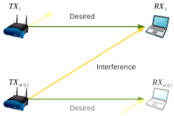
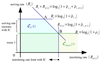
Figure 1: Rate region with IC: When a receiver RX$i$ is capable of IC, its achievable rate depends on both the serving rate rate $R_{i}$ as well as the rate $R_{\sigma(i)}$ on the interfering link. The total rate region, which includes the options of both reuse 1 and treating interference as noise as well as joint detection, is non-convex.

More sophisticated methods, such as power control and rate splitting as used in the well-known Han-Kobayashi (HK) method [21], can also be incorporated into this methodology. For example, to incorporate the HK technique, the transmitter TX$i$ would splits its transmissions into “private” and “public” parts and the decision variable $x_{i}$ for that link would be a vector including the private and public rates and their power allocations. However, for simplicity, we do not simulate this scenario.

III Message Passing Algorithms

III-A Graphical Model Formulation

As mentioned in the Introduction, graphical models provide a general and systematic approach for distributed optimization problems where the objective function admits a factorization into terms each with small numbers of variables [6, 7]. The optimization (1) with objective function (2) is ideally suited for this methodology.

To place the optimization problem into the graphical model formalism, we define a factor graph $G=(V,E)$, which is an undirected bipartite graph whose vertices consists of $n$ variable nodes associated with the decision variables $x_{i}$, $i=1,\ldots,n$, and $n$ factor nodes associated with factors $f_{i}$, $i=1,\ldots,n$. There is an edge between $x_{\ell}$ and $f_{i}$ if and only $x_{\ell}$ appears as an argument in $f_{i}$ – namely if $\ell=i$ or $\ell=\sigma(i)$.

As an example of the factor graph consider the network in the top panel of Fig. 2 with $n=6$ links. Each link has a transmitter and receiver and the diagram indicates both the serving and interfering links. The factor graph representation is shown in the bottom panel where there is one variable, $x_{i}$, and one factor, $f_{i}$, for each link $i=1,\ldots,n$.

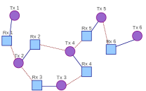
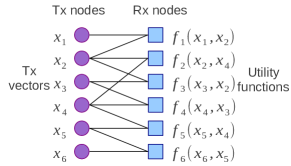
Figure 2: Example factor graph representation of a network: The top panel shows an example network with $n=6$ links, each with a transmitter and receiver. Solid lines indicate serving links and dotted lines indicate interfering links. The bottom panel shows its factor graph representation.

III-B Max-Sum Loopy BP

Once the optimization problem has been formulated as a graphical model, we can apply the standard max-sum loopy BP algorithm. A general description of the max-sum algorithm can be found in any standard graphical models text such as [6, 7]. For the dominant interferer optimization problem, the max-sum algorithm can be implemented as shown in Algorithm 1.

Loopy BP is based on iteratively passing “messages” between the variables and factor nodes. For the interferer problem, the messages are passed between the receivers RX$i$ and transmitters TX$j$ where TX$j$ is either the serving transmitter or dominant interferer of RX$i$.

Each message is a function of the scheduling decision $x_{j}$. The message function from TX$j$ to RX$i$ is denoted $\mu_{j\rightarrow i}(x_{j})$ and represents an estimate of the value of TX$j$ selecting the scheduling decision $x_{j}$. This message can thus be interpreted as a sort of “soft” request-to-send. We use the term “soft” since the message ascribes a value to each possible scheduling decision. Similarly, the messages from RX$i$ to TX$j$ is denoted $\mu_{j\leftarrow i}(x_{j})$ and has a role has both a “soft” clear-to-send and channel quality indicator (CQI).

Algorithm 1 Max-sum loopy BP for scheduling

{Initialization at the RX }

for all RX$i$ do

     $\mu_{i\rightarrow i}(x_{i})\leftarrow 0$

     $\mu_{j\rightarrow i}(x_{j})\leftarrow 0$ for $j=\sigma(i)$

end for

repeat

     { Receiver half round }

     for all RX$i$ do

         $j\leftarrow\sigma(i)$

         $\mu_{i\leftarrow i}(x_{i})\leftarrow\max_{x_{j}}f_{i}(x_{i},x_{j})+\mu_{j\rightarrow i}(x_{j})$

         $\mu_{j\leftarrow i}(x_{j})\leftarrow\max_{x_{i}}f_{i}(x_{i},x_{j})+\mu_{i\rightarrow i}(x_{i})$

     end for

     

     { Transmitter half round }

     for all TX$j$ do

         $H_{j}(x_{j})\leftarrow\mu_{j\leftarrow j}(x_{j})+\sum_{i:j=\sigma(i)}\mu_{j\leftarrow i}(x_{j})$

         $\mu_{j\rightarrow j}(x_{j})\leftarrow H_{j}(x_{j})-\mu_{j\leftarrow j}(x_{j})$

         for all $i$ s.t. $j=\sigma(i)$ do

              $\mu_{j\rightarrow i}(x_{j})\leftarrow H_{j}(x_{j})-\mu_{j\leftarrow i}(x_{j})$

         end for

     end for

until max number of iterations

{ Final scheduling decision }

for all TX$j$ do

     $H_{j}(x_{j})\leftarrow\mu_{j\leftarrow j}(x_{j})+\sum_{i:j=\sigma(i)}\mu_{j\leftarrow i}(x_{j})$

     $\widehat{x}_{j}\leftarrow\mathop{\mathrm{arg\,max}}_{x_{j}}H_{j}(x_{j})$

end for

As shown in Algorithm 1, the messages at the receiver are initialized at zero and then iteratively updated in a set of rounds. Each round consists of two halves: In the first half, the receivers send messages to the transmitters and, in the second half, the transmitters send messages back to the receivers. The process is a repeated for a fixed number of iterations, and the final messages are used to compute the scheduling decision at the transmitters.

III-C Optimality under the Dominant Interferer Assumption

We will discuss more detailed issues in implementing the algorithm momentarily. But, we first establish an important optimality, which is the main justification for the algorithm.

Theorem 1

Consider the message passing max-sum algorithm, Algorithm 1, applied to the optimization (1) with the objective function (2) for any utility functions $f_{i}(x_{i},x_{\sigma(i)})$ and dominant interferer selection function $\sigma(i)$. Then, if all messages $\mu_{i\rightarrow j}(x_{i})$ and $\mu_{i\leftarrow j}(x_{i})$ are fixed-points of the algorithm, the resulting scheduling decisions $\widehat{x}_{j}$ are globally optimal solutions to (1) in that

$$F(\widehat{\mathbf{x}})\geq F(\mathbf{x}),$$

for all other scheduling decision vectors $\mathbf{x}$.

Proof:

See Appendix A. $\Box$

The theorem shows that if the max-sum algorithm converges to a fixed point, the solution will be optimal. Remarkably, this result applies to arbitrary utility functions as long as the dominant interferer assumption is valid. In particular, the result applies to even non-convex utilities such as the ones arising in the IC problem. The result is unexpected since loopy BP is generally only guaranteed to be optimal in graphs with no cycles, and the factor graph we are considering may not be acyclic.

Of course, the theorem does not imply the convergence of the algorithm. Indeed, since the graph has cycles, the algorithm may not converge. However, the iterations of loopy can be “slowed down” using fractional updates with the same fixed points to improve convergence at the expense of increased number of iterations. However, as we will see in the simulations, convergence does not appear to be an issue in the cases we examine.

III-D Implementation Considerations

We conclude with a brief discussion of some of the practical considerations in implementing the message-passing algorithm in commercial cellular systems.

• Communication overhead: Most important, it is necessary to recognize that the message-passing needed for the proposed algorithm would require additional control channels not present in current cellular standards such as LTE or UMTS. New control channels would be needed to communicate the rounds of messaging prior to each scheduling decision. However, similar messages have been proposed in Qualcomm’s peer-to-peer system, FlashLinQ [30], and also appear in some optimized CSMA algorithms such as [31]. Under the dominant interferer assumption, the communication overhead may particularly small since each receiver must send and receive messages to and from at most two transmitters in each round (the serving transmitter and the dominant interferer). However, each message is an entire function, so the message must in principle contain a value for each possible $x_{i}$. However, if the number of values $x_{i}$ is small, or the function can be well-approximated in some simple parametric form, the overall communication per round overhead will be low. Moreover, as we will see in the simulations, very small numbers of rounds are typically needed; sometimes as small as one or two.

• Computational requirements: The computational requirements are low. The transmitter must simply sum functions, and the receivers must perform one-dimensional optimizations. Thus, as long as the sets of possibilities for each $x_{i}$ is small, the computation will be minimal.

• Channel and queue state information: The utility $f_{i}(x_{i},x_{j})$ is generally based on the rate achievable at RX$i$ as a function of the scheduling decisions at both the serving transmitter TX$i$ and the dominant interferer TX$j$. Thus, for the receiver to perform the optimization in the message passing algorithm, the receiver must generally know the channel state from the both the serving and interfering channels along with noise from all other sources. This channel state can be estimated from pilot or reference signals which are already transmitted in most cellular systems. However, the utility function will also generally depend on the queue state at the transmitter, particularly, the priorities and size of packets in the transmit buffer. This information must thus be passed, somehow, to the receiver. Cellular systems such as LTE already pass such information in the uplink through buffer status reports [15], however a similar channel would need to be placed in the downlink for this message passing algorithm to work.

• Synchronization: Since the message passing loopy BP algorithm is based on coordinated scheduling, there is an implicit assumption of synchronization. In a system such as LTE, this would require synchronization at the subframe level, where the subframes are 1ms. Since the intended use case for such coordinated scheduling applications is for small cell systems (e.g. 100 to 200m cell radii), such synchronization accuracy is reasonable.

IV Simulation Results

We validate the max-sum loopy BP algorithm for interference cancellation in two simulations. In both cases, we consider static optimizations of log utility, $U(R_{i})=\log R_{i}$, which is the proportion fair metric [28]. For the link-layer model, we assume that the rate region is described by the Shannon capacity with a loss of 3dB and there is a maximum spectral efficiency of 5 bps/Hz. The maximum spectral efficiency in practice is determined by the maximum constellation, which itself is usually limited by the receiver dynamic range. In the implementation of loopy BP, we assume a discretization of the rates using logarithmic spacing of the 25 rate points from zero to the maximum spectral efficiency. In practice, one should use the discrete modulation and coding scheme (MCS) values that are available at the link layer. In LTE, there are approximately 30 such MCS values [32].

Note that the final rates $\widehat{x}_{j}$ from Algorithm 1 may not be feasible, unless the algorithm has been run to convergence. To evaluate the algorithm prior to convergence, we obtain a feasible point from the values $\widehat{x}_{j}$ at the end of the algorithm as follows: At each receiver RX$i$, if $(\widehat{x}_{i},\widehat{x}_{\sigma(i)})\in{\mathcal{C}}(i)$ (that is, the rate pair is feasible), we take the rate $R_{i}=\widehat{x}_{i}$. Otherwise we take $R_{i}$ to be the largest value with $R_{i}\leq\widehat{x}_{i}$ and $(R_{i},\widehat{x}_{\sigma(i)})\in{\mathcal{C}}(i)$. It is simple to show that the resulting set of rates, $(R_{i},R_{\sigma(i)})$, is feasible for all $i$. This final projection step can be performed with local information only.

IV-A 3GPP Femtocellular Apartment Model

In our first simulation, we use a simplified version of an industry standard model [5] for validating ICIC algorithms of femtocells in densely packed apartments. The apartments are assumed to be laid out in a 4x4 grid, each apartment being 10x10m. In 10 of the 16 apartments, we assume there is an active link with a femto base station and mobile (user equipment or UE in 3GPP terminology). The femtos are assumed to operate in closed access mode so that a femto UE can only connect to the femto base station in its apartment. This restricted association is a major source of strong interference in femtocellular networks and thus a good test case for IC. The complete list of simulation parameters are given on the Table II.

Parameter	Value
Network topology	$4\times 4$ apartment model,with active links in 10 of the 16 apartments.
Bandwidth	5 MHz
Wall loss	10 dB
Lognormal shadowing	10 dB std. dev.
Path loss	$38.46+20\log_{10}(R)+0.7R$ dB, $R$ distance in meters.
Femto BS TX power	0 dBm
Femto UE noise figure	4 dB

TABLE I: Simulation parameters for apartment model.

Fig. 5 shows the cumulative probability distribution of resulting spectral efficiencies (bits/sec/Hz) based on 100 random drops of the network. In this figure, IC is compared against reuse 1 where no IC is used and all links transmit on the same bandwidth, treating interference as noise. We see that for cell edge users (defined as users in the lowest 10% of rates), there is a gain of almost 4 times in the rate by employing IC. Hence, IC has the potential for significant value for improving rates in such femtocellular scenarios, particularly for mobiles in strong interference.

Also shown in Fig. 5 is a comparison of the optimal rate selection against the selection from max-sum loopy BP run for 4 iterations. We see there is an exact match. In fact, even after only 1 iteration there is a minimal difference. The optimal rate selection is found as follows: For each RX$i$, the rate pair $(R_{i},R_{\sigma(i)})$ must be either in the reuse 1 region ${\mathcal{C}}_{\rm reuse1}(i)$ or the joint detection region ${\mathcal{C}}_{\rm IC}(i)$. Since there are two choices for each link, there are a total of $2^{n}$ choices in the network. For each of the $2^{n}$ choices, the total rate region is convex and we can maximize the utility over that region. For the optimal rate selection, we repeat the convex optimization for every one of $2^{n}$ choices and select the one with the maximum total utility. Obviously, the max-sum loopy BP algorithm is much simpler.

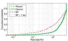
Figure 3: Simulation with 3GPP apartment model: Plotted are the distribution of rates (bps/Hz) over 100 drops. We see that IC provides significant gains particularly at the cell edge. Moreover, even one iteration of max-sum loopy BP finds near-optimal rates for the non-convex optimization problem.

IV-B Road Network with Mobility

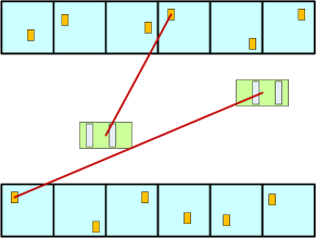
Figure 4: Road network model: Using open-access femtocells within apartments may enable low-cost wide-area cellular coverage. However, mobility within small cells can result in significant interference as handover delays cause mobile users to drag into neighboring cells.

A second case of strong interference in femto- or picocellular networks is handover delays. When cells are small, handovers are frequent. Also, since femtocells are not be directly into the operator’s core network [33], the handovers between femtocells or from the femtocells to the macrocell may be significantly delayed [3]. Due to the delays, the mobile may drag significantly into cells other than the serving cell, exposing the mobile to strong interference.

To evaluate the ability of IC to mitigate this strong interference, we considered a road network model shown in Fig. 4. A similar model was considered in [34]. In this model, the transmitters are femtocells placed in apartments at two sides of the road. The receivers are mobile on the road with a random velocity between 15 and 25 m/s. Each mobile is initially connected to the strongest serving cell. After the connection, we let mobiles to move for a time uniformly distributed between 0 and 1 second to model the effect of delayed handover. We then perform a static simulation taken at this snapshot in time. The complete list of simulation parameters are given on the Table I, which are loosely based on the path loss models in [5].

Parameter	Value
Network topology	10 Tx’s in/on apartments by the road, 10 mobile Rx’s on the road in periodic
Road width	10 m
Road length	50 m periodicity
Apartment dim.	10 m width and 20 m length
Bandwidth	5 MHz
Wall loss	0 dB
Lognormal shadowing	10 dB std. dev.
Path loss	$10+37\log_{10}(R)$ dB, $R$ distance in meters.
Rx velocity	15 - 25 m/s
Femto BS TX power	0 dBm
Femto UE noise figure	4 dB

TABLE II: Simulation parameters for road model.

Fig. 5 shows the distribution of rates based on 100 random drops. Again, we see that IC provides significant improvement in cell edge rate: the 10% rate is increased by more than a factor of 3. In fact, even the median rate is increased almost twofold. In addition, max-sum loopy BP finds near optimal rates.

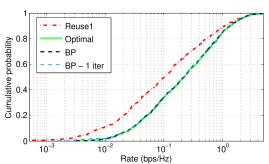
Figure 5: Simulation for the road network model: Plotted are the distribution of rates (bps/Hz) over 100 drops. Again, we see that IC provides significant gains in rates throughout the rates, but particularly at the cell edge. Moreover, max-sum loopy BP finds near-optimal selections after only 1 iteration.

V Conclusions

A general methodology based on max-sum loopy BP is presented for wireless scheduling and resource allocation problems in networks where each link has at most one dominant interferer. The algorithm is extremely general and can incorporate advanced link-layer mechanisms available in modern cellular systems. Moreover, the method is completely distributed, requires low communication overhead and minimal computation. In addition, although we did not establish the convergence of the algorithm, we have shown that if it converges, the result is guaranteed to be globally optimal. Remarkably, this result holds for arbitrary problems, even when the problems are non-convex, the only requirement being the dominant interferer assumption.

The method was applied to systems with IC. We propose that when IC is available at the link-layer, rate control as opposed to power control can provide an effective mechanism for interference coordination. Moreover, the optimal rate selection is performed extremely well by max-sum loopy BP. Simulations of the algorithm in femtocellular networks demonstrate considerable improvement in capacity from the addition of IC for handling both restricted association and mobility. In addition, loopy BP appears to provide near optimal performance with only one or two rounds of messaging, thus making the methodology extremely attractive for practical networks.

Appendix A Proof of Theorem 1

We begin by reviewing the following well-known result from [35, 18]: Let $G_{U}=(V,E_{U})$ be an undirected graph with vertices $V=\{1,\ldots,n\}$, and suppose that a function $F(\mathbf{x})$ admits a pairwise factorization of the form

$$F(\mathbf{x})=\sum_{(i,j)\in E_{U}}f_{ij}(x_{i},x_{j}),$$ (11)

for some set of functions $f_{ij}(x_{i},x_{j})$. Note that the graph $G_{U}$ is not the factor graph. One can then apply max-sum loopy BP to attempt to perform the optimization

$$\widehat{\mathbf{x}}=\mathop{\mathrm{arg\,max}}_{\mathbf{x}}F(\mathbf{x}).$$ (12)

It is well-known that max-sum loopy BP will provide the optimal solution when $G_{U}$ has no cycles. However, our analysis requires the following.

Theorem 2 (​[18])

Consider max-sum loopy BP applied to the optimization (12) to an arbitrary pairwise objective function of the form (11). Suppose that each connected component of the undirected graph $G_{U}$ has at most one cycle. Then, if the belief messages are fixed points of max-sum loopy BP, the corresponding solution $\widehat{\mathbf{x}}$ is optimal in that $F(\widehat{\mathbf{x}})\geq F(\mathbf{x})$ for all vectors $\mathbf{x}$.

Now, the function (2) we are interested in is a special case of the form (11), so we need to show that the corresponding undirected graph, $G_{U}$, has the same single cycle property. The undirected graph for the objective function (2) is simple to describe: First let $G_{D}=(V,E_{D})$ be the directed graph with vertices $V=\{1,\ldots,n\}$ and directed edges

$$E_{D}=\{(\sigma(i),i),~{}i=1,\ldots,n\}.$$

Then, if $G_{U}=(V,E_{U})$ is the corresponding undirected graph to $G_{D}$, then it is also the undirected graph for the objective function (2). For illustration, Fig. 6 shows the directed graph $G_{D}$ for the example network mentioned earlier in Fig. 2. Note that there is a directed edge from $j$ to $i$ if and only if TX$j$ is the dominant interferer of RX$i$. Since each receiver has at most one dominant interferer, each node in $G_{D}$ has at most one incoming edge. That is, the in-degree is at most one for all nodes. This property will be key.

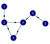
Figure 6: Directed graph for the example network in Fig. 2. There is a directed edge from $j$ to $i$ if and only if $j=\sigma(i)$, namely TX$j$ is the dominant interferer of RX$i$.

To apply Theorem 2, we need to show that each connected component of $G_{U}$ has at most one cycle. We begin with the following lemma.

Lemma 1

Consider any path $P_{M}=(i_{1},i_{2},...,i_{M})$, in the undirected graph $G_{U}$. Then either $(i_{2},i_{1})\in E_{D}$ or $(i_{M-1},i_{M})\in E_{D}$. That is, either the first or last segments of the path are pointing “outwards”.

Proof:

The proof follows by induction. For $M=2$, either $(i_{2},i_{1})$ or $(i_{1},i_{2})$ must be a directed edge. Now suppose the the lemma is true for all paths of length $M-1$, and consider a path of length $M$. If $(i_{2},i_{1})\in E_{D}$ we are done, so suppose $(i_{2},i_{1})\not\in E_{D}$. Then, applying the induction hypothesis to $P_{M-1}$ shows that $(i_{M-2},i_{M-1})$ must be a directed edge. But, since the node $i_{M-1}$ can have at most one incoming edge, $(i_{M-1},i_{M})$ must be outgoing and hence in $E_{D}$. So, we have shown that either $(i_{2},i_{1})\in E_{D}$ or $(i_{M-1},i_{M})\in E_{D}$. $\Box$

We wow return to the graph $G_{U}$ and show that each connected component can have at most one cycle. We prove the property by contradiction. Assume there are two loops in the same connected component of $G_{U}$:

$$L = (i_{1},i_{2},...,i_{K},i_{1})$$

$$J = (j_{1},j_{2},...,j_{M},j_{1}),$$

with no repetitions of points within each loop, aside from the first and last points. Now there are three possibilities as shown in Fig. 7: (a) The two loops have no common point, (b) one common point and (c) two or more common points. We show each of these possibilities leads to a contradiction.

Figure 7: Possible positions of two loops in the same connected component.

Case (a) No common points

By assumption, $L$ and $J$ are in the same connected component, so there must be a path in the undirected graph between between one point in $L$ and a second point in $J$. Without loss of generality (WLOG), we can assume the path goes from $i_{1}$ to $j_{1}$ and we will write the path as

$$P=(i_{1}=k_{1},k_{2},\ldots,k_{N}=j_{1}).$$

We can construct this path such that, aside from $i_{1}$ and $j_{1}$, this path has no common points with the loops $L$ or $J$. Now, by Lemma 1, either $(k_{2},k_{1})$ or $(k_{N-1},k_{N})$ is a directed edge (i.e. in $E_{D}$). WLOG suppose $(k_{2},k_{1})\in E_{D}$; the other case is similar. The point $k_{1}$ would correspond to point B in Fig. 7 with the loop on the right being loop $L$. Thus $k_{1}=i_{1}$ has an incoming edge from $k_{2}$. But Lemma 1 applied to the path $L$ implies that there must be an incoming edge from either $i_{2}$ or $i_{K}$. When combined with the incoming edge from $k_{2}$, $i_{1}$ has more than one incoming edge, which is impossible.

Case (b) One common point

WLOG we can assume that the point $i_{1}=j_{1}$ is the common point in loops $L$ and $J$. The point is shown as A in Fig. 7. Applying Lemma 1 to both loops $L$ and $J$ show that there must be at least one incoming edge into point A from each loop. Thus, A has more than one incoming edge, which again is a contradiction.

Case (c) Two or more common points

Taking a minimal common path, and possibly rearranging the indexing, we can assume that the first $N$ points of the loops $L$ and $J$ are common so that

$$i_{1}=j_{1},\ldots,i_{N}=j_{N},$$

but $i_{N+1}\neq j_{N+1}$, and $i_{K}\neq j_{M}$. The situation is depicted in Fig. 7, where point A corresponds to $i_{1}$ ($=j_{1}$) and B corresponds to $i_{N}$ ($=j_{N}$). Applying Lemma 1 to the path along the common segment from A to B,

$$P=(i_{1},\ldots,i_{N})=(j_{1},\ldots,j_{N}),$$

implies that either $(i_{2},i_{1})$ or $(i_{N-1},i_{N})$ is a directed edge. WLOG assume $(i_{N-1},i_{N})$ is a directed edge, creating an incoming edge into point B (the point with index $i_{N}=j_{N}$). Since any node can have at most one incoming edge, both the edges $(i_{N},i_{N+1})$ in loop $L$ and $(j_{N},j_{N+1})$ in loop $J$ must be directed edges outgoing from $i_{N}=j_{N}$. Now consider the two paths from $i_{N}=j_{N}$ back to $i_{1}=j_{1}$ along loops $L$ and $J$. From Lemma 1, since the initial segments, $(i_{N},i_{N+1})$ in loop $L$ and $(j_{N},j_{N+1})$ in loop $J$, are directed edges, the final segments $(i_{K},i_{1})$ and $(j_{M},j_{1})$ must also be directed edges. Thus, there are two incoming edges into point A (the point with index $i_{1}=j_{1}$). This is a contradiction.

Thus, all three cases are impossible, and we have proven by contradiction that any connected component of $G_{U}$ can have at most one cycle. We can therefore apply Theorem 2 and the proof of Theorem 1 is complete.

References

- [1] V. Chandrasekhar, J. G. Andrews, and A. Gatherer, “Femtocell networks: A survey,” IEEE Comm. Mag., vol. 46, no. 9, pp. 59–67, Sep. 2009.
- [2] D. López-Pérez, A. Valcarce, G. de la Roche, and J. Zhang, “OFDMA femtocells: A roadmap on interference avoidance,” IEEE Comm. Mag., vol. 47, no. 9, pp. 41–48, Sep. 2009.
- [3] J. G. Andrews, H. Claussen, M. Dohler, S. Rangan, and M. C. Reed, “Femtocells: Past, present, and future,” IEEE J. Sel. Areas Comm., vol. 30, no. 3, Apr. 2012.
- [4] 3GPP, “New Work Item Proposal: Enhanced ICIC for non-CA based deployments of heterogeneous networks for LTE,” RP-100372, 2010.
- [5] Femto Forum, “Interference management in OFDMA femtocells,” Whitepaper available at www.femtoforum.org, Mar. 2010.
- [6] M. J. Wainwright and M. I. Jordan, Graphical Models, Exponential Families, and Variational Inference, ser. Foundations and Trends in Machine Learning. Hanover, MA: NOW Publishers, 2008, vol. 1.
- [7] B. J. Frey, Graphical Models for Machine Learning and Digital Communication. MIT Press, 1998.
- [8] M. Chiang, “Distributed network control through sum product algorithm on graphs,” in Proc. IEEE Globecom, vol. 3, Nov. 2002, pp. 2395 – 2399.
- [9] S. Sanghavi, D. Malioutov, and A. Willsky, “Belief propagation and LP relaxation for weighted matching in general graphs,” in Proc. NIPS, December 2007.
- [10] M. Bayati, D. Shah, and M. Sharma, “Max-product for maximum weight matching: convergence, correctness and LP duality,” IEEE Trans. Inform. Theory, vol. 54, no. 3, pp. 1241–1251, March 2008.
- [11] I. Sohn, S. H. Lee, and J. G. Andrews, “A graphical model approach to downlink cooperative MIMO systems,” IEEE Globecom, 2010.
- [12] S. Rangan and R. Madan, “Belief propagation methods for intercell interference coordination,” in Proc. IEEE Infocom, Shanghai, China, Apr. 2011.
- [13] ——, “Belief propagation methods for intercell interference coordination in femtocell networks,” IEEE J. Sel. Areas Comm., vol. 30, no. 3, pp. 631–640, Apr. 2012.
- [14] S. Rangan, A. K. Fletcher, V. K. Goyal, and P. Schniter, “Hybrid generalized approximation message passing with applications to structured sparsity,” in Proc. IEEE Int. Symp. Inform. Theory, Cambridge, MA, Jul. 2012, pp. 1241–1245.
- [15] E. Dahlman, S. Parkvall, J. Sköld, and P. Beming, 3G Evolution: HSPA and LTE for Mobile Broadband. Oxford, UK: Academic Press, 2007.
- [16] L. Tassiulas and A. Ephremides, “Stability properties of constrained queueing systems and scheduling policies for maximum throughput in multihop radio networks,” IEEE Trans. Automat. Control, vol. 37, pp. 1936–1948, 1992.
- [17] A. Stolyar, “On the asymptotic optimality of the gradient scheduling algorithm for multi-user throughput allocation,” Oper. Res., 2005.
- [18] Y. Weiss and W.T.Freeman, “On the optimality of solutions of the max-product belief-propagation algorithm in arbitrary graphs,” IEEE Trans. Inform. Theory, vol. 47, no. 2, pp. 736–744, Feb. 2001.
- [19] R. Ahlswede, “Multi-way communication channels,” in Proc. IEEE Int. Symp. Inform. Theory, Armenian S.S.R., Sep. 1971, pp. 23–52.
- [20] T. M. Cover and J. A. Thomas, Elements of Information Theory. New York: John Wiley & Sons, 1991.
- [21] T. Han and K. Kobayashi, “A new achievable rate region for the interference channel,” IEEE Trans. Inform. Theory, vol. 27, no. 1, pp. 49–60, Jan. 1981.
- [22] R. Etkin, D. Tse, and H. Wang, “Gaussian interference channel capacity to within one bit,” IEEE Trans. Inform. Theory, vol. 54, no. 12, pp. 5534 –5562, Dec. 2008.
- [23] S. Rangan, “Femto-macro cellular interference control with subband scheduling and interference cancelation,” in Proc. IEEE Globecom, Miami, FL, Dec. 2010, pp. 695–700.
- [24] J. G. Andrews, “Interference cancellation for cellular systems: A contemporary overview,” IEEE Wireless Comm., vol. 12, no. 2, pp. 19–29, Apr. 2005.
- [25] G. Boudreau, J. Panicker, N. Guo, R. Chang, N. Wang, and S. Vrzic, “Interference coordination and cancellation for 4G networks,” IEEE Comm. Mag., vol. 47, no. 4, pp. 74–81, Apr. 2009.
- [26] Z. Shi and M. C. Reed, “Iterative maximal ratio combining channel estimation for multiuser detection on a time frequency selective wireless CDMA channel,” in Proc. IEEE Wireless Communications and Networking Conference, Hong Kong, Mar. 2007.
- [27] M. Chiang, P. Hande, T. Lan, and C. W. Tan, “Power control in wireless cellular networks,” Foundation and Trends in Networking, vol. 2, no. 4, pp. 381–533, Jul. 2008.
- [28] F. P. Kelly, A. K. Maulloo, and D. K. H. Tan, “Rate control for communication networks: shadow prices, proportional fairness and stability,” Journal of the Operational Research Society, vol. 49, no. 3, pp. 237–252, Mar. 1998.
- [29] S. Shakkottai and R. Srikant, Network Optimization and Control, ser. Foundations and Trends in Networking. NOW Publishers, 2007.
- [30] S. Tavildar, S. Shakkottai, T. Richardson, J. Li, R. Laroia, and A. Jovicic, “FlashLinQ: A synchronous distributed scheduler for peer-to-peer ad hoc networks,” in Proc. Allerton Conf. Comm. Control & Comp., Allerton, IL, Oct. 2010.
- [31] J. Ni and R. Srikant, “Distributed CSMA/CA algorithms for achieving maximum throughput in wireless networks,” in Proc. Information Theory and Applications Workshop, San Diego, CA, Jan. 2009.
- [32] 3GPP, “Evolved Universal Terrestrial Radio Access (e-utra); Physical Channels and Modulation,” TS 36.211 (release 10), 2012.
- [33] ——, “UTRAN architecture for 3G Home Node B (HNB); stage 2,” TS 25.467 (release 9), 2010.
- [34] S. Rangan and E. Erkip, “Hierarchical Mobility in Dense Cellular Networks via Relaying,” in Proc. Globecomm, Houston, TX, Dec. 2011.
- [35] Y. Weiss, “Correctness of Local Probability Propagation in Graphical Models with Loops,” Neural Comp., vol. 12, no. 1, pp. 1–41, Jan. 2000.