Symmetric excitation and de-excitation of a cavity QED system

Abstract

We calculate the time evolution of a cavity-QED system subject to a time dependent sinusoidal drive. The drive is modulated by an envelope function with the shape of a pulse. The system consists of electrons embedded in a semiconductor nanostructure which is coupled to a single mode quantized electromagnetic field. The electron-electron as well as photon-electron interaction is treated exactly using “exact numerical diagonalization” and the time evolution is calculated by numerically solving the equation of motion for the system’s density matrix. We find that the drive causes symmetric excitation and de-excitation where the system climbs up the Jaynes-Cummings ladder and descends back down symmetrically into its original state. This effect persists even in the ultra-strong coupling regime where the Jaynes-Cummings model is invalid. We investigate the robustness of this symmetric behavior with respect to the drive de-tuning and pulse duration.

I Introduction

A quantum two level system (TLS) interacting with a single mode of a quantized electromagnetic field is a central topic within the scope of circuit quantum electrodynamics (QED). Typically, the light-matter interaction is weak enough to warrant the use of some version of the Jaynes-Cummings (JC) model Jaynes and Cummings (1963) to describe both static Wallraff et al. (2004); Fink et al. (2008); Kasprzak et al. (2010) and time dependent systems Alsing et al. (1992); Bishop et al. (2008); De Liberato et al. (2009); Schmidt et al. (2010). However, recent progress in the field of circuit QED has enabled the fabrication of ultra-small mode-volume cavities where the light-matter interaction strength can be a considerable fraction of a cavity photon energy. In this regime, evidence of the breakdown of the JC-model (with the rotating wave approximation) has been observed in superconducting Niemczyk et al. (2010) and semiconductor systems Günter et al. (2009); Anappara et al. (2009).

In previous work, we have gone beyond the TLS approximation and solved the many-body Schrödinger equation exactly for electrons embedded in a semiconductor nanostructure, subject to a single mode quantized EM field and an external classical magnetic field Jonasson et al. (2012a). The electron-electron and photon-electron interactions were treated exactly using exact numerical diagonalization (for details see Ref. Jonasson et al. (2012b)). We predicted the failure of the JC-model (including anti-resonance terms) at high coupling strengths for a static and closed system. Here, we expand on that work by adding an explicit time dependence to the total Hamiltonian and investigate its dynamical properties.

We investigate the effects of time dependent addition to the total Hamiltonian which does not depend on the cavity photon creation or annihilation operators. In the language of the JC-model, this means that we are perturbing the atomic term of the total Hamiltonian as opposed to the cavity field or interaction term. The time dependent term is a sinusoidal drive which is modulated by an envelope function which varies slowly compared with other characteristic time scales of the system.

The paper is organized as follows. In Sec. II we describe the static part of the Hamiltonian which contains the geometry of the semiconductor nanostructure as well as the electron-electron and photon-electron interaction. In Sec. III we add a time dependent drive to the total Hamiltonian and introduce the time dependent observables we are interested in and how we calculate them. Results and concluding remarks are presented in Secs. IV and V respectively.

II Description of the static system

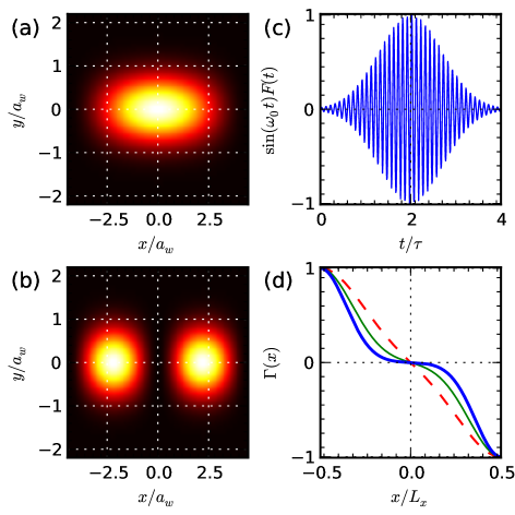
Figure 1: (Color online) Charge densities for the SES’s $|1\rangle$ (a) and $|2\rangle$ (b) in arbitrary units for zero magnetic field. Dark is low density and bright is high. (c), sinusoidal pulse with a Gaussian envelope function with $\alpha=10$ which gives $10$ complete oscillations in the time interval $\tau$. (d), spatial variation of the drive potential $\Gamma(x)$ for $\beta_{x}L_{x}=3$ (dashed red line), $\beta_{x}L_{x}=4$ (thin green line) and $\beta_{x}L_{x}=5$ (thick blue line). $\Gamma$ is homogeneous in the $y$-direction so a 3D plot is not needed.

We split the static part of the system’s Hamiltonian $\mathcal{H}_{0}$ into four terms,

$$\mathcal{H}_{0}=\mathcal{H}_{e}+\mathcal{H}_{\textrm{EM}}+\mathcal{H}_{p}+\mathcal{H}_{d}\ .$$ (1)

They are the electronic part of the Hamiltonian ($\mathcal{H}_{e}$), the cavity field Hamiltonian ($\mathcal{H}_{\textrm{EM}}$), the paramagnetic ($\mathcal{H}_{p}$) and diamagnetic ($\mathcal{H}_{d}$) electron-photon interaction terms. The electronic part can be written as

$$\mathcal{H}_{e} =\mathcal{H}_{w}+\mathcal{H}_{\textrm{Coul}}$$ (2)

$$=\sum_{i}E_{i}d^{\dagger}_{i}d_{i}+\frac{1}{2}\sum_{ijrs}\langle ij|V_{\textrm{Coul}}|rs\rangle d_{i}^{\dagger}d_{j}^{\dagger}d_{s}d_{r}\ ,$$ (3)

where $\mathcal{H}_{w}$ is the Hamiltonian of a finite quasi-one-dimensional (Q1D) quantum wire with hard walls at $x=\pm L_{x}/2$ and a parabolic confinement in the $y$-direction with characteristic energy $\hbar\Omega_{0}$, containing several non-interacting electrons. The wire is subject to an external classical magnetic field $\mathbf{B}=\nabla\times\mathbf{A}_{\textrm{ext}}=B\mathbf{\hat{z}}$. With the magnetic field, the characteristic energy in the $y$-direction is modified to $\hbar\Omega_{w}=\hbar\sqrt{\Omega_{0}^{2}+\omega_{c}^{2}}$, where $\omega_{c}$ is the cyclotron frequency $\omega_{c}=qB/m^{*}$, with $q$ the positive elementary charge and $m^{*}$ the electron effective mass. A natural length scale is $a_{w}=\sqrt{\hbar/(m^{*}\Omega_{w})}$. $d^{\dagger}_{i}$ and $d_{i}$ are fermionic creation and annihilation operators of the single electron eigenstates (SES) $|i\rangle$, with energies $E_{i}$, which include the effect of the external magnetic field. Figs. 1(a) and 1(b) show the charge density of the two lowest SES for zero magnetic field.

$\mathcal{H}_{\textrm{Coul}}$ contains the effect of the Coulomb interaction with the kernel

$$V_{\mathrm{Coul}}(\mathbf{r},\mathbf{r}^{\prime})=\frac{q^{2}/(4\pi\varepsilon)}{\sqrt{(x-x^{\prime})^{2}+(y-y^{\prime})^{2}+\eta^{2}}}\ ,$$ (4)

where $\eta$ is a small convergence parameter to regulate the singularity at $\mathbf{r}=\mathbf{r}^{\prime}$. We denote the many electron eigenstates of $\mathcal{H}_{w}$ as $|\mu\rangle$ (we use Latin indices for single-electron states and Greek ones for the many-electron states) with the energy $E_{\mu}$. These states are simply Slater determinants in the SES’s $|i\rangle$. We denote eigenstates of $\mathcal{H}_{e}$ as $|\mu)$ (denoted now with a rounded right bracket) with energy $\tilde{E}_{\mu}$. The states $|\mu\rangle$ and $|\mu)$ are connected via a unitary transformation $|\mu)=\mathcal{V}|\mu\rangle$. We calculate $\mathcal{V}$ by diagonalizing $\mathcal{H}_{e}$ in the basis of the eigenstates of $\mathcal{H}_{w}$. Where needed, we use the notation $|\mu)_{N}$ to denote the $\mu$-th electronic state containing $N$ electrons. For example, $|4)_{2}$ is the fourth lowest two electron state. Note that we have a closed system so the number of electrons is a conserved quantity.

The cavity field EM Hamiltonian can be written as $\mathcal{H}_{\textrm{EM}}=\hbar\omega_{p}a^{\dagger}a$ where $a^{\dagger}$ and $a$ are bosonic creation and annihilation operators of a cavity photon with energy $\hbar\omega_{p}$. The photon energy is typically chosen such that it matches a transition energy in the quantum wire (i.e. the photon field is near a resonance).

By taking the long wavelength approximation for the quantized EM field, its vector potential can be written as $\mathbf{A}_{\mathrm{E}M}=A_{\mathrm{EM}}\mathbf{\hat{e}}(a+a^{\dagger})$ with $\mathbf{\hat{e}}$ a unit vector pointing in the field’s direction of polarization. The paramagnetic interaction term can then be written as

$$\mathcal{H}_{p}=\mathcal{E}_{c}\sum_{ij}d^{\dagger}_{i}d_{j}g_{ij}(a+a^{\dagger})$$ (5)

where we have defined the electron-photon coupling strength $\mathcal{E}_{c}=qA_{\textrm{EM}}\Omega_{w}a_{w}$, which is the characteristic energy scale for the photon-electron interaction. We have also introduced an effective dimensionless coupling tensor (DCT)

$$g_{ij}=\frac{a_{w}}{\hbar}\mathbf{\hat{e}}\cdot\langle i|\bm{\pi}|j\rangle\ ,$$ (6)

defining the coupling of individual single-electron states $|i\rangle$ and $|j\rangle$ by the photonic mode where $\bm{\pi}=\mathbf{p}+q\mathbf{A}_{\textrm{ext}}$ is the mechanical momentum. It is useful to generalize $g_{ij}$ to

$$\mathcal{G}_{\mu\nu}=\sum_{i,j}g_{ij}(\mu|d_{i}^{\dagger}d_{j}|\nu)$$ (7)

so that $\mathcal{G}_{\mu\nu}$ is the DCT which defines the coupling of many-electron states $|\mu)$ and $|\nu)$ by the photon field. From Eq. (7) we see that $\mathcal{G}_{\mu\nu}$ depends on the geometry of the quantum wire and on the magnetic field. Note that the action of $d_{i}$ and $d_{i}^{\dagger}$ is only known in the $\left\{|\mu\rangle\right\}$ basis (of non-interacting Fock states). To calculate for example $d_{i}|\mu)$ we have to use $d_{i}|\mu)=d_{i}\mathcal{V}|\mu\rangle$. This definition of $\mathcal{G}_{\mu\nu}$ makes comparison with the JC-model easy, since the coupling energy $\mathcal{E}_{\textrm{JC}}$ in the JC model (in the $\mathcal{E}_{\textrm{JC}}\sigma_{x}(a+a^{\dagger})$ term) is related to the DCT via $\mathcal{E}_{\textrm{JC}}=|\mathcal{G}_{\kappa\lambda}|\mathcal{E}_{c}$ where $|\kappa)$ and $|\lambda)$ are the two states chosen for the TLS approximation (active states) Jonasson et al. (2012a). We will refer to $\mathcal{E}_{c}$ as the electron-photon coupling strength (or simply the coupling strength) and $\mathcal{E}_{\textrm{JC}}$ as the effective coupling strength.

The diamagnetic interaction term can be written as

$$\mathcal{H}_{d}=\frac{\mathcal{E}_{c}^{2}}{\hbar\Omega_{w}}\mathcal{N}_{e}\left[\left(a^{\dagger}a+\frac{1}{2}\right)+\frac{1}{2}\left(a^{\dagger}a^{\dagger}+aa\right)\right]\ ,$$ (8)

where $\mathcal{N}_{e}$ is the electron number operator.

Now that we have defined all the terms in (1), we can put the results together and expand $\mathcal{H}_{0}$ in the $\left\{|\mu)\right\}$ basis,

$$\mathcal{H}_{0}=\sum_{\mu}\tilde{E}_{\mu}|\mu)(\mu|+\hbar\omega_{p}a^{\dagger}a+\sum_{\mu\nu}\mathcal{E}_{c}\mathcal{G}_{\mu\nu}|\mu)(\nu|(a+a^{\dagger})$$

$$+\frac{\mathcal{E}_{c}^{2}}{\hbar\Omega_{w}}N_{e}\left\{\left(a^{\dagger}a+\frac{1}{2}\right)+\frac{1}{2}\left(a^{\dagger}a^{\dagger}+aa\right)\right\}$$ (9)

where $N_{e}$ is the number of electrons in the system.

Next we proceed to expand $\mathcal{H}_{0}$ in a basis containing a preset number of photons $\left\{|M\rangle\right\}$ (eigenstates of $a^{\dagger}a$ with eigenvalue $M$). We have then expanded $\mathcal{H}_{0}$ in the complete orthonormal basis $\left\{|\breve{\alpha}\rangle\right\}=\left\{|\mu)\otimes|M\rangle\right\}$. From the diagonalization process we obtain a unitary transformation $\mathcal{U}$ which satisfies $\mathcal{U}|\breve{\alpha}\rangle=|\breve{\alpha})$ where $|\breve{\alpha})$ are eigenstates of $\mathcal{H}_{0}$ satisfying $\mathcal{H}_{0}|\breve{\alpha})=\breve{E}_{\alpha}|\breve{\alpha})$. The states $|\breve{\alpha})$ are then used as a basis in time dependent calculations which are covered in section III.

III Time dependent Hamiltonian

Now we add a time dependent drive to the Hamiltonian in the form (in first quantization)

$$W(t)=W_{0}\Gamma(x,y)\sin(\omega_{0}t)F(t)\ ,$$ (10)

where $W_{0}$ is the drive amplitude which has units of energy, $\Gamma(x,y)$ contains the spatial dependence of $W(t)$ and $F(t)$ is an envelope function for the sinusoidal term $\sin(\omega_{0}t)$. We choose $\omega_{0}$ such that $\hbar\omega_{0}$ matches some transition energy in the quantum wire (i.e. the drive is near a resonance). We will refer to $\hbar\omega_{0}$ ($\omega_{0}$) as the drive energy (frequency). In this work we will choose $F(t)$ to be a pulse which varies slowly on the timescale $2\pi/\omega_{0}$ and satisfies $F(\pm\infty)=0$ and $F(t)\leq 1$. An example of such an envelope function is a Gaussian

$$F(t)=e^{-(t-t_{0})^{2}/\tau^{2}}\ ,$$ (11)

where $\tau\gg 2\pi/\omega_{0}$. It is useful to define the quantity $\alpha=\omega_{0}\tau/(2\pi)$ which gives the number of oscillations within the time interval $\tau$ (see Fig. 1(c)). Note that a larger value of $\alpha$ translates into a longer pulse (not a faster oscillating pulse). As for the geometric part we will use

$$\Gamma(x,y)=-e^{-\beta_{x}^{2}(x-L_{x}/2)^{2}}+e^{-\beta_{x}^{2}(x+L_{x}/2)^{2}}\ ,$$ (12)

so $\Gamma(x,y)=\Gamma(x)$ is a sum of two Gaussians of opposite sign that are centered on the opposite end of the quantum wire (see Fig. 1(d)). The reasons for this choice of $\Gamma$ is that it couples the time dependent part of the Hamiltonian strongly to a cavity field that is polarized in the $x$-direction.

To add $W(t)$ to $\mathcal{H}_{0}$, we need to calculate the second quantization generalization of $W(t)$ in the $\left\{|\mu)\right\}$ basis using

$$\mathcal{W}(t)= \sum_{ij\mu\nu}\langle i|W|j\rangle(\mu|d_{i}^{\dagger}d_{j}|\nu)|\mu)(\nu|$$

$$= W_{0}\sin(\omega_{0}t)F(t)\sum_{\mu\nu}\Gamma_{\mu\nu}|\mu)(\nu|$$ (13)

where the matrix element $\Gamma_{\mu\nu}$ characterizes the coupling of individual Coulomb interacting many-electron states $|\mu)$ and $|\nu)$ by $\mathcal{W}(t)$. In (13), $\mathcal{W}(t)$ is simply a unit operator in the photon Fock space since it does not depend on $a$ or $a^{\dagger}$.

Now that we have the matrix representation of the total Hamiltonian $\mathcal{H}=\mathcal{H}_{0}+\mathcal{W}(t)$, we can calculate the time evolution of the system by integrating the equation of motion

$$i\hbar\frac{\partial\rho}{\partial t}=\left[\mathcal{H},\rho\right]\ .$$ (14)

where $\rho$ is the density matrix of the system. This is done numerically using a Crank-Nicolson method. We let the system start out in the ground state and investigate its excitation by $\mathcal{W}(t)$.

The observables we are interested in are the mean number of photons $\langle N\rangle(t)$ and energy $E(t)=\langle\mathcal{H}\rangle(t)$ which can be calculated using $\langle\mathcal{A}\rangle(t)=\textrm{Tr}\left[\rho(t)\mathcal{A}(t)\right]$ where $\mathcal{A}$ is some observable.

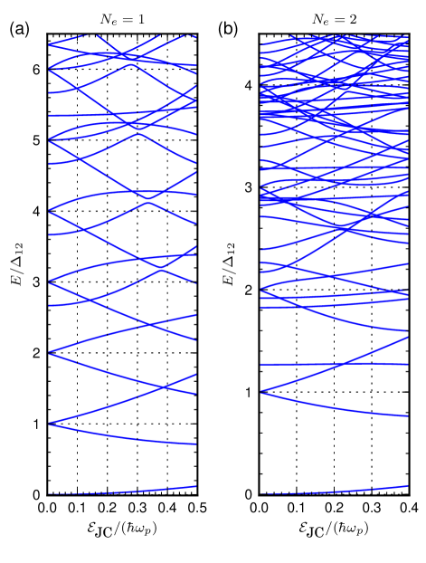
Figure 2: (Color online) (a), Energy spectra for one electron at zero external magnetic field as a functions of the effective coupling strength $\mathcal{E}_{\textrm{JC}}=|\mathcal{G}_{12}|\mathcal{E}_{c}$ where $|\mathcal{G}_{12}|=0.300$ and $\Delta_{12}=0.197$ meV. (b), same as in (a), but for two electrons with $|\mathcal{G}_{12}|=0.676$ and $\Delta_{12}=0.521$ meV. Note that the energy spectrum has been shifted so that the ground state has zero energy at zero coupling strength.

IV Results

Throughout this section, we use $L_{x}=300$ nm, $\hbar\Omega_{0}=1.0$ meV, $\beta_{x}L_{x}=4$, $\alpha=90$, $m^{*}=0.067m_{e}$ and $\varepsilon=12.4\varepsilon_{0}$ (GaAs parameters). Unless otherwise stated, both the cavity photon energy $\hbar\omega_{p}$ as well as the drive energy $\hbar\omega_{0}$ are on resonance between the electronic states $|1)$ and $|2)$ with de-tuning $\delta=10^{-4}\Delta_{12}$, where $\Delta_{12}=\tilde{E}_{2}-\tilde{E}_{1}$ is the energy difference between the two lowest electronic eigenstates. We let the system start out in its ground state and always use an envelope function of the form in (11). Where needed, we will differentiate the de-tuning of the cavity field and the drive energy as $\delta_{p}$ and $\delta_{d}$ respectively. We will only consider $x$-polarization for two reasons. First, it couples the states $|1)$ and $|2)$ strongly (large $\left|\mathcal{G}_{12}\right|$). Second, the quantum wire is approximately (for small magnetic field) harmonic in the $y$-direction. We want to compare our results to simpler TLS models and for a TLS approximation to be applicable, there needs to be some anharmonicity present to minimize excitation to states outside of the TLS Hilbert space.

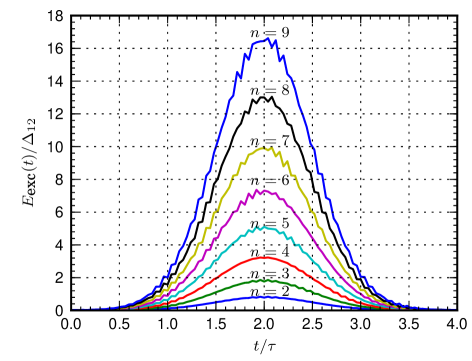
Figure 3: (Color online) Excitation energy vs time for a system containing one electron at zero magnetic field. The envelope function $F(t)$ is a Gaussian of the form in (11) with $t_{0}=2\tau$ and $\alpha=90$, giving $90$ oscillations in the time interval $\tau$. The effective coupling strength is $\mathcal{E}_{\textrm{JC}}/(\hbar\omega_{p})\simeq 0.13$. The system starts out in the ground state at $t=0$. The different curves are for different $W_{0}$ (see Eq. (13)) where $W_{0}/\Delta_{12}=n\times 0.428$.

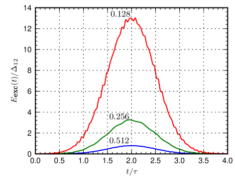
Figure 4: (Color online) Excitation energy vs time for a system containing one electron at zero magnetic field. All parameters are the same as in Fig. 3 except $\mathcal{E}_{\textrm{JC}}$ is varied instead of $W_{0}$. Note that changing the electron-photon coupling shifts the ground state energy as can be seen in Fig. 2. That is why the above energy is shifted by the ground state energy $\breve{E}_{0}$. The three different numerical values $0.128$, $0.256$ and $0.512$ are the value of $\mathcal{E}_{\textrm{JC}}/(\hbar\omega_{p})$ used for for the corresponding curve.

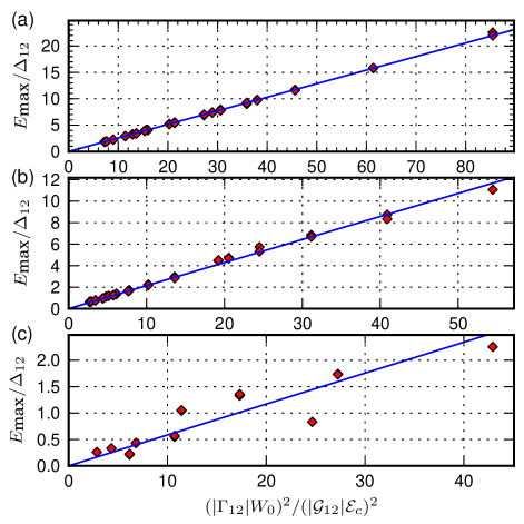
Figure 5: (Color online) Maximum excitation energy for many values of $\mathcal{E}_{c}$, $W_{0}$ and $B$ with $\mathcal{E}_{c}$ and $W_{0}$ in the range of that of Figs. 3 and 4 and $B$ in the range $0.0$-$0.5$ T. Results are shown for one (a), two (b) and three (c) electrons with $52$, $47$ and $18$ data points respectively (some data-points overlap and are not distinguishable on the graphs). The blue lines are least square fit with (15) giving $A(1)=0.26$, $A(2)=0.21$ and $A(3)=0.058$. The results are very robust for one and two electrons but start to show significant deviations for three electrons.

Fig. 2 shows energy spectra for $\mathcal{H}_{0}$ with one and two electrons. From the figure we can see $4$-$6$ of the lowest polariton pairs in the JC-ladder, along with other states that are not a part of the TLS approximation. Note how much denser the two electron spectrum is. The range of coupling strength is similar to what we use for time dependent calculations later on.

Fig. 3 shows the excitation energy $E_{\textrm{exc}}(t)=E(t)-E(t=0)$ of the system as a function of time for various driving field amplitudes ($W_{0}$). The most interesting aspect of the figure is the symmetric excitation and de-excitation of the system. What is happening is that the system is climbing up the Jaynes-Cummings ladder and descending back down symmetrically. This would not be surprising for a low coupling strength where both the anti-resonant and diamagnetic terms of the electron-photon interaction Hamiltonian can be ignored. In that case, when both the drive and photon energy are on resonance, it is possible to find quasi stationary states which are periodic in time (see Ref. Alsing et al. (1992)). The effect of the envelope function is then to adiabatically tune the system’s quasi ground state. The adiabatic nature of the envelope function prevents transitions beyond this slowly shifting quasi ground state. When the envelope function goes to zero again the system is adiabatically shifted to its original state. Like mentioned earlier, this behavior is expected at low coupling strength, however, for the plots in Fig. 3, the electron-photon coupling is rather large ($\mathcal{E}_{\textrm{JC}}/(\hbar\omega_{p})\simeq 0.13$). In fact, for this coupling strength, a visible deviation from the JC-model is apparent in Fig. 2(a) where the polariton splittings don’t show the characteristic linear $\pm\sqrt{n}\mathcal{E}_{\textrm{JC}}$ splittings which we expect from the JC-model (for further comparison with the JC-model, see Ref. Jonasson et al. (2012a) or Jonasson (2012)). Another interesting aspect of Fig. 3 is that the value of the maximum energy $E_{\textrm{max}}$ at $t\simeq 2\tau$ scales quadratically with $W_{0}$. This will be addressed later in this work.

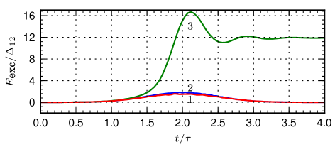
Figure 6: (Color online) Excitation energy vs time. All three plots are for one electron, $B=0$, $W_{0}=0.24$ meV, $\mathcal{E}_{c}=0.08$ meV and $\left|\mathcal{G}_{12}\right|=0.3$, giving $\mathcal{E}_{\textrm{JC}}/(\hbar\omega_{p})\simeq 0.13$. Curve $1$ shows the exact results using our full model. Curve $2$ shows results obtained using a TLS approximation using only two states for the electron Hilbert space basis where the diamagnetic interaction term is ignored. Curve $3$ shows results using a TLS approximation including the diamagnetic interaction term. Note how the TLS approximation with diamagnetic term drastically overestimates the excitation energy and how the system is not symmetrically de-excited.

Fig. 4 shows the excitation energy of the system as a function of time for various effective coupling strengths ($\mathcal{E}_{\textrm{JC}}$), keeping the drive amplitude ($W_{0}$) constant at $W_{0}/\Delta_{12}\simeq 3.4$. Note that in $\mathcal{E}_{\textrm{JC}}=\left|\mathcal{G}_{12}\right|\mathcal{E}_{c}$, only $\mathcal{E}_{c}$ can be varied since $\mathcal{G}_{\mu\nu}$ depends only on geometry. The same excitation and de-excitation pattern is apparent, even for the ultrastrong coupling $\mathcal{E}_{\textrm{JC}}/(\hbar\omega_{p})=0.512$. We did not perform calculations for higher coupling because of issues with numerical convergence at higher coupling strengths (see Ref. Jonasson et al. (2012b) for detailed convergence calculations). Counter-intuitively, the maximum excitation energies at $t\simeq 2\tau$ in Fig. 4 is proportional to the inverse square of the coupling strength $\mathcal{E}_{c}$. We can therefore see that the maximum excitation energy follows the relationship $E_{\textrm{max}}\propto(W_{0}/\mathcal{E}_{c})^{2}$.

By doing calculations for many different values of $W_{0}$, $\mathcal{E}_{c}$ and magnetic field strength, we were able to deduce the relationship

$$\frac{E_{\textrm{max}}}{\Delta_{12}}=A(N_{e})\left(\frac{\left|\Gamma_{12}\right|W_{0}}{\left|\mathcal{G}_{12}\right|\mathcal{E}_{c}}\right)^{2}\ .$$ (15)

Where $A(N_{e})$ is a dimensionless constant that depends only on the number of electrons but not on the geometry of the system. Deducing the $(W_{0}/\mathcal{E}_{c})^{2}$ relationship was straightforward since $W_{0}$ and $\mathcal{E}_{c}$ are both parameters we can freely change. However, to show the $|\Gamma_{12}/\mathcal{G}_{12}|^{2}$ relationship we had to vary the matrix elements $\Gamma_{12}$ and $\mathcal{G}_{12}$. We did this by doing calculations for different magnetic field strengths (see Fig. 5). Varying the magnetic field changes the geometry of the system and thereby changes both $\Gamma_{12}$ and $\mathcal{G}_{12}$. By doing this we eliminate the possibility of the symmetric excitation de-excitation behavior being a special case of the geometry we have chosen or due to the time reversal symmetry (which the magnetic field breaks). Note that changing the magnetic field and electron number alters the energy spectrum so $\Delta_{12}$ is not always the same. From Fig. 5 we see that the agreement with Eq. (15) is very good for one and two electrons while large deviation is apparent for three electrons. The reason for this is that for more electrons, the energy spectrum is much denser and previously inactive states start to have bigger influence. Least square fit with (15) gives $A(1)=0.26$, $A(2)=0.21$ and $A(3)=0.058$ which shows that a larger electron number translates into a weaker response to the drive.

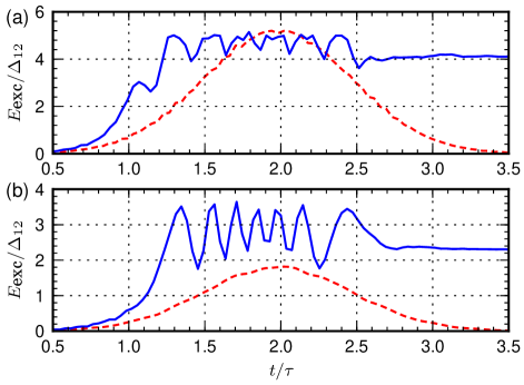
Figure 7: (Color online) (a), excitation energy vs time for two values of drive de-tuning for one electron with $\mathcal{E}_{\textrm{JC}}/(\hbar\omega_{p})\simeq 0.13$, $W_{0}/\mathcal{E}_{c}=5$ and $B=0$. The two curves are for a de-tuning $\delta_{d}/\Delta_{12}=0.02$ (red-dashed) and $\delta_{d}/\Delta_{12}=0.05$ (solid blue), giving $\lambda\simeq 5.0$ and $\lambda=1.0$ respectively. The symmetric behavior is lost in the latter case. (b), Same as in (a) except $\mathcal{E}_{\textrm{JC}}/(\hbar\omega_{p})\simeq 0.26$ and $W_{0}/\mathcal{E}_{c}=3$. The two curves are for a de-tuning $\delta_{d}/\Delta_{12}=0.01$ (green-dashed) and $\delta_{d}/\Delta_{12}=0.1$ (solid black), giving $\lambda\simeq 14$ and $\lambda\simeq 1.4$ respectively. The symmetric behavior is lost in the latter case. Note that in both (a) and (b), the cavity photon de-tuning is held constant at $\delta_{p}=10^{-4}\Delta_{12}$

We find that the mean number of photons follows the same relationship as the energy

$$N_{\textrm{max}}=A(N_{e})\left(\frac{\left|\Gamma_{12}\right|W_{0}}{\left|\mathcal{G}_{12}\right|\mathcal{E}_{c}}\right)^{2}\ ,$$ (16)

where $N_{\textrm{max}}$ is the peak value of $\langle N\rangle(t)$. The constant of proportionality $A(N_{e})$ is the same as for (15).

Because the geometric dependence of Eqs. (15) and (16) is encoded in the two matrix elements $\Gamma_{12}$ and $\mathcal{G}_{12}$ it is tempting to say that a TLS description is applicable and we can ignore the inactive electronic states (all electronic states except $|1)$ and $|2)$). This is true for small coupling strength where the JC-model can be used and the diamagnetic interaction term is small. However, as can be seen from Fig. 6, a TLS description starts to fail at coupling strengths of $\mathcal{E}_{\textrm{JC}}/(\hbar\omega_{p})\sim 0.1$. What is surprising in Fig. 6 is that for coupling strength $\mathcal{E}_{\textrm{JC}}/(\hbar\omega_{p})\sim 0.1$, including the diamagnetic interaction term in a TLS model gives much less accurate results than if it is ignored. This behavior is observed when $\mathcal{E}_{\textrm{JC}}/(\hbar\omega_{p})\gtrsim 0.10$. It seems that the effects of the diamagnetic interaction term are canceling the effects of the inactive states. However, for even higher coupling strengths, the TLS model (with or without the diamagnetic interaction term) will fail because it can’t account for the complicated effect of inactive states in an energy spectrum such as the ones in Fig. 2.

We will end this section by investigating the robustness of the results. Fig. 7 shows results with different values of the drive de-tuning. We find that symmetric excitation de-excitation behavior persists as long as

$$\lambda\equiv\frac{\Delta_{12}}{\delta_{d}}\left(\frac{\left|\mathcal{G}_{12}\right|\mathcal{E}_{c}}{\left|\Gamma_{12}\right|W_{0}}\right)^{2}\gg 1\ .$$ (17)

We also investigated what is the minimum pulse length needed to observe the symmetric behavior (see Fig. 8). We find that the minimum value $\alpha\simeq 10$ is needed. This means that we need at least $10$ complete oscillations within the time period $\tau$. This is the same value of $\alpha$ which is used for illustrative purposes in Fig. 1(c).

Throughout this work we used a Gaussian shaped envelope function. It is worth noting that the above mentioned symmetric behaviour is not a special case for this choice. We tested this by varying the envelope function such that $F(t)=\exp{\left\{-|t-t_{0}|^{n}/\tau^{n}\right\}}$, with $n$ in the range $1$-$5$. This change does affect the shape of the excitation energy curves such as those in Figs. 3 and 4 but the excitation and de-excition is still symmetric and has the same maximum value as with a Gaussian shaped envelope function.

Finally, we note that so far we have only used envelope functions that are symmetric around $t=t_{0}$. We found that relaxing this restriction does change the symmetric exciation and de-excitation behavior such as not being symmetric about $t\simeq t_{0}$ anymore, but as long as the envelope function is slowly varying, the system still ends up in the same state as it started in (the ground state).

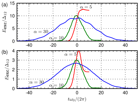
Figure 8: (Color online) Excitation energy vs time for different values of $\alpha$. (a), one electron, $B=0.2$ T, $\mathcal{E}_{c}=0.16$ meV, $W_{0}=0.48$ meV, $\Delta_{12}=0.172$ meV and $\mathcal{E}_{\textrm{JC}}/(\hbar\omega_{p})=0.245$. (b), two electrons, $B=0.1$ T, $\mathcal{E}_{c}=0.08$ meV, $W_{0}=0.32$ meV, $\Delta_{12}=0.511$ meV and $\mathcal{E}_{\textrm{JC}}/(\hbar\omega_{p})=0.101$. In both (a) and (b), we see that in order observe the symmetric behavior, we need to have $\alpha\gtrsim 10$. Note that the time axis has been shifted in both (a) and (b) such that the pulse maximum is at $t=0$.

V Concluding remarks

We have described a method to compute the time evolution of a many-body, multi level, Coulomb interacting electronic system which is coupled to a single-mode quantized EM field. The Hamiltonian contains explicit time dependence on the form of a sinusoidal drive which is modulated by an envelope function. The envelope function is a Gaussian shaped pulse that varies slowly compared to characteristic time scales of the system. Both the drive frequency and the cavity photon frequency are on resonance with a transition in the electronic system. The only approximations which are made are the finite size of single- and many-body bases as well as the finite precision of the numerical integration. The convergence with respect to these parameters is carefully controlled.

We observed a symmetric excitation and de-excitation of the system where the drive causes the system to climb up the Jaynes-Cummings ladder. When the pulse dies out, the system descends down the ladder back to its original (ground) state. This is not a simple adiabatic effect because even though the envelope function varies slowly, the drive frequency matches that of the cavity photons as well as a transition in the electronic nanostructure.

We found that when the system exhibits symmetric excitation and de-excitation, the maximum expectation values of the energy and photon number follow a simple relationship which is independent of the specific geometry, but does depend on the number of electrons in the system. The effect is very robust for one electron, slightly less so for two electrons and considerable deviation is observed for three electrons. This is due to the much denser many electron energy spectra, where states which are not a part of the Jaynes-Cummings ladder start to have greater influence.

We compared the results of our full model to that of a TLS model. We did this by doing calculations where only two states are used as a basis for the electronic part of the Hamiltonian. We found that for the relatively weak coupling strength $\mathcal{E}_{\textrm{JC}}\simeq 0.13$, including the diamagnetic interaction term gives much worse results than if it is ignored. The results of the TLS model without the diamagnetic term is in agreement with the results of the full model.

We tested robustness of the above mentioned symmetric behavior with respect to the magnitude of the drive de-tuning. We found that the maximum allowed value of the relative de-tuning was $1$-$2$%. Note that this value depends strongly on geometry, coupling- and drive amplitude (see Eq. (17)). Finally, we investigated how long the pulse needs to be to see the symmetric effect. We found that approximately $10$ complete oscillations are needed within the time period $\tau$, where $\tau$ characterizes the duration of the pulse via Eq. (11).