Formation of proto-clusters and star formation within clusters: apparent universality of the initial mass function ?

Abstract

Context. It is believed that the majority of stars form in clusters. Therefore it is likely that the gas physical conditions that prevail in forming clusters largely determine the properties of stars that form in particular, the initial mass function.

Aims. We develop an analytical model to account for the formation of low-mass clusters and the formation of stars within clusters.

Methods. The formation of clusters is determined by an accretion rate, the virial equilibrium as well as energy and thermal balance. For this latter, both molecular and dust cooling are considered using published rates. The star distribution is computed within the cluster using the physical conditions inferred from this model and the Hennebelle & Chabrier theory.

Results. Our model reproduces well the mass-size relation of low mass clusters (up to few $\simeq 10^{3}$ M_⊙ of stars corresponding to about five times more gas) and an initial mass function that is $i)$ very close to the Chabrier IMF, $ii)$ weakly dependent on the mass of the clusters, $iii)$ relatively robust to (i.e. not too steeply dependent on) variations of physical quantities such as accretion rate, radiation, and cosmic ray abundances.

Conclusions. The weak dependence of the mass distribution of stars on the cluster mass results from the compensation between varying clusters densities, velocity dispersions, and temperatures that are all inferred from first physical principles. This constitutes a possible explanation for the apparent universality of the IMF within the Galaxy although variations with the local conditions may certainly be observed.

1 Introduction

Since the pioneering work of Salpeter (1955), the origin of the initial mass function (IMF; e.g. Kroupa 2002, Chabrier 2003) remains one of the most fundamental questions in astrophysics. More particularly, its apparent universality, Bastian et al. (2010), remains debated and challenging. Indeed, as described by these authors, the IMF has now been determined in many environments, and although some of the results may be interpreted as evidence of variations, neither systematic, nor undisputable evidence for such variations of the IMF are unambiguously reported. Therefore even if, as it will probably eventually turn out, some variations are finally clearly established, in many environments, the variations of the IMF remains limited.

Various theories have been proposed to explain the apparent constancy of the IMF. These theories often rely on the independence of the Jeans mass on the density. For example, Elmegreen et al. (2008) computed the gas temperature in various environments and found a very weak dependence of the Jeans mass on the density since the latter increases with temperature. Bate (2009) and Krumholz (2011) estimated the temperature in a massive collapsing clump in which the gas is heated by the radiative feedback due to accretion onto the protostars. Bate (2009) found that in the vicinity of the protostars, the Jeans mass is typically proportional to $\rho^{1/5}$. While this later idea is interesting, it raises a few questions. First, the first generation of stars is, at least at the beginning of the process, not influenced by the radiative feedback. Second, even when the stars start forming, the regions in which heating is important remain limited to the neighborhood of the protostars. Thus it is not yet demonstrated that most stars will be affected by this effect and that it is sufficient to make the IMF universal. Moreover the recent simulations by Krumholz et al. (2012) suggest that indeed the gas temperature is much too high when radiative feedback is included, leading to an IMF that is inconsistently shifted toward high masses. On the contrary when outflows are included, the radiation can escape along the outflow cavities and they obtain IMF which are close to the observed one.

Another type of arguments invokes the variation of the effective polytropic index, $\gamma$, which in particular presents a local minimum at about $10^{5}$ cm^-3 (e.g. Larson 1985) due to the transition between cooling dominated lines and dust. This in particular has been proposed by Bonnell et al.(2006) and Jappsen et al. (2005). However, it remains unclear that it is actually the case because the various simulations did not clearly establish that changing the cloud initial conditions while keeping a fixed equation of state would lead to a CMF peaking at the same mass. Moreover Hennebelle & Chabrier (2009) compare their predictions with the peak position found in numerical simulations of Jappsen et al. (2005) and find a good agreement. Yet in the Hennebelle & Chabrier theory, a local minimum of $\gamma$ does not determine the peak of the CMF which still depends on the Mach number for example.

More generally, these theoretical arguments assume that the Jeans mass is the only parameter that determines the IMF. This sounds rather unlikely because a distribution like the IMF is not entirely determined by a single parameter (peak position, width, and slope at high masses), moreover, analytical theories like the one proposed by Hennebelle & Chabrier (2008, HC2008) and Hopkins (2012) explicitly depend on the Mach number. Although no systematic exploration of the Mach number influence on the core mass function has been performed in numerical simulations, Schmidt et al. (2010) have explored the role of the forcing of the turbulence. They showed in particular that the core mass function (CMF) is quite different when the forcing is applied in pure compressible or pure solenoidal modes. This clearly suggests that the CMF is affected by the velocity field. Even more quantitatively, Schmidt et al. (2010) found a good agreement between the CMF they measure and the analytical model of HC2008 which seemingly confirms the Mach number dependence of this model. From a physical point of view, it is well established that the density probability distribution function (PDF) is strongly related to the Mach number (Vázquez-Semadeni 1994, Padoan et al. 1997, Passot & Vázquez-Semadeni 1998, Kim & Ryu 2005, Kritsuk et al. 2007, Federrath et al. 2008, Audit & Hennebelle 2010). Accordingly, because the density PDF is clearly important with regard to the Jeans mass distribution within the cloud, it would be quite surprising if the Mach number had no influence on the CMF.

Another line of explanation regarding the universality of the IMF has been proposed by HC2008, who argue that because the peak position of the IMF is proportional to the mean Jeans mass and inversely proportional to the Mach number, there is a compensation because from Larson relations, the density decreases when the velocity dispersion increases and thus the mean Jeans mass and the Mach number increase at the same time (see Eq. 47 of HC2008 and figure 8 of HC2009). One problem of this explanation is, however, that Larson relations present a high dispersion and that there are clouds for example, with the same density but different Mach numbers that may therefore lead to different IMF in particular at low masses.

Generally speaking, all approaches that attempt to understand the universality of the IMF suffer from the variability of the star-forming cloud conditions. This clearly emphasizes the need for a better understanding of the physical conditions under which stars form. In this respect, an important key is that most stars (say 50-70%) seem to form in clusters (Lada & Lada 2003, Allen et al. 2007), which is a strong motivation to study the formation of clusters. Note, however, that Bressert et al. (2010) moderate this picture to some extent.

A word of caution is nonetheless necessary here. The constancy of the IMF is debated and some observations even in the Galaxy may indicate that some variability has already been observed (see e.g. Cappellari et al. 2011 for early types galaxies). For a discussion and good summary on this problem we refer the reader to Dib et al. (2010). Moreover, these authors have developed an analytical model of the core formation within proto-clusters that takes into account the turbulent formation of dense cores as well as their accretion of gas that could modify the CMF and lead to IMF variability. Along a similar line, Dib et al. (2007) showed how the coalescence of cores can explain the development of a top-heavy IMF.

In this paper, we first develop an analytical model for the formation of clusters, more precisely, the formation of proto-clusters, i.e. the gas dominated phase that eventually leads to star-dominated clusters. Our model relies on the gas accretion onto the proto-clusters from parent clumps that feed them in mass and in energy. This allows us to predict the physical quantities such as radius, mean density, and velocity dispersion within the proto-clusters as a function of the accretion rate. By comparing with the data of embedded clusters from Lada & Lada (2003), we can estimate the accretion rate onto these proto-clusters and verify that our model fits the observational data well. In a second step, we calculate the gas temperature within the proto-clusters by computing the various heating and cooling, and we apply a time-dependent version of the model of HC2008 to predict the mass spectrum of the self-gravitating condensations and in particular to study their variability with proto-cluster masses and accretion rates.

The second part of the paper presents the analytical model of the proto-clusters and the comparison with the observational data. The third part is devoted to the calculation of the thermal balance as well as to the description of the HC2008 theory. In the fourth part, we calculate the mass spectra within the proto-clusters. The fifth section concludes the paper.

2 Analytical model for low mass cluster formation

Clusters are likely to play an important role for the formation of stars in the Milky Way (e.g. Lada & Lada 2003) and probably for most galaxies. It seems therefore a necessity, in order to understand how star forms to obtain a good description of the gas physical conditions within proto-clusters. For that purpose, we develop here an analytical model that is based on the following general ideas. First, proto-clusters are initially likely to be gravitationally bound entities. However, proto-clusters are not collapsing, which means that a support is actually compensating gravity, which we assume is the turbulent dispersion. This will be expressed by applying the virial theorem to the proto-cluster. Because turbulence is continuously decaying with a characteristic time on the order of the crossing time, it must be continuously sustained. We assume that the continuous accretion of gas into the proto-cluster from the parent clump is the source of energy. Indeed, accretion-driven turbulence has been recently proposed to be at play in various contexts (Klessen & Hennebelle 2010, Goldbaum et al. 2011). Our first step is therefore to discuss the parent clumps and the resulting accretion rate onto the proto-cluster. Once an accretion rate is inferred, an energy balance can be written and together with the relation obtained from the virial theorem lead to a link between the mass, the radius, and the velocity dispersion within the cluster.

2.1 Parent cloud, protocluster and accretion rate

2.1.1 Definitions and assumptions

Let us consider a clump of mass $M_{c}\simeq 10^{3}-10^{6}M_{\odot}$ and radius $R_{c}$ that follows Larson relations (Larson 1981, Falgarone et al. 2004, Falgarone et al. 2009):

$$n_{c}=n_{0}\left({R_{c}\over 1{\rm pc}}\right)^{-\eta_{d}},\,\,\sigma_{\rm rms}=\sigma_{0}\left({R_{c}\over 1{\rm pc}}\right)^{\eta},$$ (1)

where $n_{c}$ is the clump gas density and $\sigma_{rms}$ the internal rms velocity. The exact values of the various coefficients remain somewhat uncertain. Originally, Larson (1981) estimate $\eta_{d}\simeq 1.1$ and $\eta\simeq 0.38$, but more recent estimates (Falgarone et al. 2004, 2009) using larger sets of data suggest that $\eta_{d}\simeq 0.7$ and $\eta\simeq 0.5$. These later values agree well with the estimate from numerical simulations of supersonic turbulence (e.g. Kritsuk et al. 2007) and we therefore use them throughout the paper although we will compare the accretion rates obtained for both sets of values.

As explained above, we consider the formation of a cluster within the parent clump. Because we are essentially considering the early phase during which the gas still dominates over the stars, we refer to it as the proto-cluster. Let $M_{*}$ be its mass and $\alpha_{*,c}=M_{c}/M_{*}$ be the ratio between the parent clump and proto-cluster masses. Let us stress that $M_{*}$ is the mass of gas within the proto-clusters and not the mass of stars. Throughout this work the star component is not considered.

Obviously, the proto-cluster is accreting from the parent clump, which is therefore regulating the rate at which matter is delivered onto the proto-cluster. The immediate question concerns then the value of the accretion rate ? To answer this we consider two different approaches. First we assume that the proto-cluster clump is undergoing Bondi-type accretion, i.e. accretion regulated by its own gravity. However because this process can be sustained only if sufficient matter is available for accretion, we also explore the possibility that the accretion onto the proto-cluster is regulated by the accretion onto the parent clumps. In this case, the accretion is due to the mechanism that is at the origin of the clump formation and that also sets the Larson relations. Both assumptions lead to similar, although not identical values and dependence.

2.1.2 Bondi-type accretion rate

The Bondi-Hoyle accretion rate that an object of mass $M_{*}$ is experiencing in a medium of density $\rho$ and sound speed $c_{s}$ is given by $\dot{M}=4\pi\rho G^{2}M_{*}^{2}/c_{s}^{3}$ (Bondi 1941). In a turbulent medium the accretion rate is not well established. While a simple expression is given by $\dot{M}=4\pi\rho G^{2}M_{*}^{2}/(c_{s}^{2}+\sigma^{2})^{3/2}$, where $\sigma$ is the velocity dispersion, Krumholz et al. (2005) obtain and discuss more refined estimates. We stress that these estimates assume that the accreting reservoir is infinite, which, as already mentioned may not be true in the present context. Moreover, these accretion rates are valid only for point masses and it is unclear whether they apply to more extended objects such as proto-clusters.

To estimate an accretion rate, here we used the modified Bondi expression. The density $\rho$ and the velocity dispersion $\sigma$ are those from the parent clump stated in Eqs. (1). Because these quantities depend on the parent clump mass, $M_{c}$, and because $M_{*}$ likely increases with $M_{c}$, it is clear that the dependence of the accretion rate is not proportional to $M_{*}^{2}$ but rather has a more shallow dependence essentially because $\rho$ and $\sigma$ decreases and increases respectively when $M_{c}$ increases. To arrive at a more quantitative estimate, we assume that $\alpha_{*,c}$ does not depend on $M_{c}$ and is therefore constant. We obtain

$$\dot{M} = {4\pi\rho G^{2}M_{*}^{2}\over\sigma^{3}}={4\pi M_{p}n_{0}G^{2}M_{c}^{2}\over\alpha_{*,c}^{2}\sigma_{0}^{3}(R/1{\rm pc})^{\eta_{d}+3\eta}}$$ (2)

$$\propto \alpha_{*,c}^{-2}M_{c}^{3(2-(\eta_{d}+\eta))\over(3-\eta_{d})}.$$

For $\eta_{d}=0.7$, $\eta=0.45$, we get $\dot{M}\propto M^{-1.1}$ while for $\eta_{d}=1.1$, $\eta=0.4$, we obtain $\dot{M}\propto M^{-0.8}$. Figure 1 shows the resulting accretion rate, BL1 and BL2 referring to the first and second sets of parameters respectively, the values $\alpha_{*,c}=3$ (upper curves) and $\alpha_{*,c}=5$ (lower curves) were used. This likely corresponds to upper values of the accretion rate because higher values of $\alpha_{*,c}$ lead to lower values of $\dot{M}$, while for lower values of $\alpha_{*,c}$, the mass within the parent clumps is equal to or even smaller than, the mass within the protocluster and it is therefore extremely unlikely that Bondi-type accretion is relevant at all.

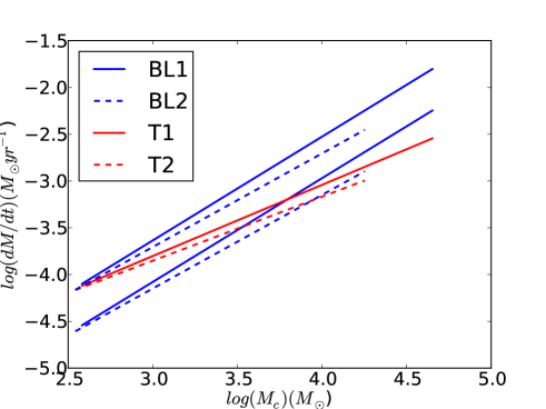
Figure 1: Accretion rate onto the proto-cluster against clump mass. BL1 and BL2 represent Bondi-Lyttleton accretion for $\eta_{d}=1.1$, $\eta=0.4$ and $\eta_{d}=0.7$, $\eta=0.45$, respectively. T1 and T2 represent the turbulent accretion rate with the same values. Upper (lower) BL curves are for parent clump over proto-cluster mass of 3 (5).

2.1.3 Turbulent accretion rate

The second type of accretion we consider is the one that is responsible for the clump formation. The exact nature of these clumps is still a matter of debate but simulations have been reasonably successful to explain at least the low-mass part of the distribution (e.g. Hennebelle & Audit 2007, Banerjee et al. 2009, Klessen & Hennebelle 2010) in which they can essentially be seen as turbulent fluctuations. In this view, as the properties of the clumps stated by Eqs. (1) are the result of the turbulent cascade, that is to say, the material within the clumps is delivered by the compressive motions of the surrounding diffuse gas, it seems reasonable to construct an accretion rate out of the Larson relations.

The clump crossing time, $\tau_{c}$ is about $2R/(\sigma/\sqrt{3})$ where the factor $\sqrt{3}$ accounts for the fact that it is the one-dimensional velocity dispersion that is relevant for estimating the crossing time.

The accretion rate of diffuse gas onto the clump is expected to be

$$\dot{M} \simeq {M_{c}\over\tau_{c}}\simeq{M_{c}\over 2R_{c}/(\sigma_{rms}/\sqrt{3})},$$

$$\simeq M_{c}^{{2-\eta_{d}+\eta\over 3-\eta_{d}}}{\sigma_{0}\over 2\sqrt{3}}\left({4\pi\over 3}n_{0}m_{p}\right)^{1-\eta\over 3-\eta_{d}}(1\,{\rm pc})^{\eta_{d}-3\eta\over 3-\eta_{d}},$$

$$= \dot{m}_{4}\left({M_{c}\over 10^{4}M_{\odot}}\right)^{\eta_{acc}},$$

$$\simeq 9\times 10^{-4}M_{\odot}\,{\rm yr}^{-1}\,\left({M_{c}\over 10^{4}M_{\odot}}\right)^{2-\eta_{d}+\eta\over 3-\eta_{d}}$$

$$\times{\sigma_{0}\over 0.8\,{\rm km\,s^{-1}}}\left({n_{0}\over 1000\,{\rm cm}^{-3}}\right)^{1-\eta\over 3-\eta_{d}},$$

where $m_{p}$ is the mass per particle. Note that to estimate $\dot{m}_{4}$ we used $\eta_{d}=0.7$ and $\eta=0.45$.

The Larson relations that describe the mean properties of the clump in which the cluster forms are likely a direct consequence of the interstellar turbulence. Thus, the accretion is likely to last a few clump crossing times, which is typically the correlation time in turbulence.

If the clump is sufficiently dense, it undergoes gravitational collapse and forms a cluster of mass $M_{*}$. Here we attempt to understand the cluster formation phase. For that purpose, we assume that:

-

as already explained it starts with a gas-dominated phase, i.e. the mass of the cluster is dominated by the mass of its gas and not its stars

-

this phase is quasi-stationary, i.e. the cluster properties evolve slowly with respect to its crossing time.

-

the accretion rate onto the cluster is comparable to the accretion rate of diffuse gas onto the clump and is therefore close to the value given by Eq. (2.1.3).

Of these three assumptions, the second one is certainly the least obvious. Indeed, initially no star will have formed by definition, while what we assume in practice regarding the accretion rate is simply that it scales as $\dot{M}\propto M^{\eta_{acc}}$ and we fit the coefficient using observed proto-clusters. Taking time-dependence into account would certainly be highly desirable at some stage but will probably not modify the results very significantly.

It is useful to express the accretion rate as a function of the proto-cluster mass and we write

$$\dot{M}=\dot{m}_{4}\left({\alpha_{*,c}\over 10^{4}M_{\odot}}\right)^{\eta_{acc}}M_{*}^{\eta_{acc}}=Q_{0}M_{*}^{\eta_{acc}}.$$ (4)

Assuming that the parameter $\dot{m}_{4}$ stays constant, this implies that the accretion rate onto the proto-clusters is controlled by $M_{c}$, the mass of their parent clumps, and thus by $\alpha_{*,c}=M_{c}/M_{*}$, which effectively quantifies the strength of the accretion onto the proto-cluster. In practice, $\dot{m}_{4}$ could vary while $\alpha_{*,c}$ would be constant, it is equivalent, however, and does not make any difference if one uses one or the other. Below we use $\alpha_{*,c}$ to quantify the accretion onto the proto-cluster.

2.2 Virial equilibrium

Because a cluster initially is a bound system, which unlike a protostellar core is not globally collapsing, it seems clear that on large scale some sort of mechanical equilibrium is established, to describe which we use the virial theorem. When applying the virial theorem to the cluster, it must be taken into account that it is gaining mass by accretion and is therefore not a close system. In Appendix A, we show that when applied to an accreting system, the expression of the virial theorem becomes

$$\dot{M}^{2}{dR_{*}^{2}\over dM_{*}}+M_{*}\sigma_{*}^{2}-3P_{\rm ram}V_{*}+E_{g}=0.$$ (5)

In this expression, $M_{*}$ is the cluster mass, $\sigma_{*}$ is the rms velocity of the gas within the cluster, $V_{*}=4\pi/3R_{*}^{3}$ is its volume, and $P_{\rm ram}$ is the external pressure exerted by the infalling clump gas onto the cluster which dominates over the thermal pressure. Assuming that the gas within the parent clumps is gravitionally attracted by the proto-cluster, the infall velocity is simply the gravitational freefall, and we obtain

$$v_{\rm inf}=\sqrt{2GM_{*}\over R_{*}}.$$ (6)

The ram pressure is given by $P_{\rm ram}=\rho_{\rm inf}v_{\rm inf}^{2}$ while the accretion rate $\dot{M}$ leads to the relation $\dot{M}=4\pi R_{*}^{2}\rho_{\rm inf}v_{\rm inf}$, therefore leading to

$$P_{\rm ram}={\dot{M}\over 4\pi R_{*}^{2}}v_{\rm inf}={G^{1/2}\dot{M}M_{*}^{1/2}\over 2\sqrt{2}\pi R_{*}^{5/2}}.$$ (7)

The gravitational energy of a uniform density sphere is well-known to be $-(3/5)GM_{*}^{2}/R_{*}$, and thus we obtain

$$\dot{M}^{2}{dR_{*}^{2}\over dM_{*}}+M_{*}\sigma_{*}^{2}-3P_{\rm ram}V_{*}-{3\over 5}{GM_{*}^{2}\over R_{*}}=0.$$ (8)

2.3 Energy balance

As stated in Eq. (8), the proto-cluster is confined by its own gravity and by the ram pressure of the incoming flow. The velocity dispersion of the gas it contains resists these two confining agents. To estimate its magnitude, we assume an equilibrium between energy injection and turbulent dissipation

$${M_{*}\sigma_{*}^{2}\over 2\tau_{\rm cct}}\simeq\dot{E}_{\rm ext}+\dot{E}_{\rm int},$$ (9)

where $\tau_{\rm cct}$ is the cluster crossing time and is about $\tau_{\rm cct}\simeq 2R_{*}/{\sigma_{*}/\sqrt{3}}$. $\dot{E}_{\rm int}$ and $\dot{E}_{\rm ext}$ are the external and internal source of energy injection which compensate the energy dissipation stated by the left side. Note that in principle a complete energy equation could be written that would entail thermal energy but also terms taking into account the expansion or contraction of the proto-cluster (see e.g. Goldbaum et al. 2011). However, the exact amount of energy dissipated by turbulence is not known to better than a factor of a few and the same is true regarding the efficiency with which the accreting gas can sustain turbulence (giving that a certain fraction can quickly dissipate in shocks). Since these two contributions are dominant, we consider a simple balance at this stage from which physical insight can be gained.

From Eq. (9), we obtain

$$\sigma_{*}^{2}\simeq\left(2\sqrt{3}R_{*}{\dot{E}_{\rm ext}+\dot{E}_{\rm int}\over M_{*}}\right)^{2/3}.$$ (10)

Note that in this work we do not consider any internal energy source such as supernova explosions, jets, winds, and ionizing radiation from massive stars, accordingly $\dot{E}_{\rm int}=0$ is assumed in this paper.

The external source of energy is generated by the accretion process itself because the kinetic energy of the infalling material triggers motion within the cluster. This energy flux is on the order of $(1/2)\dot{M}v_{\rm inf}^{2}\simeq G\dot{M}M_{*}/R_{*}$. It is slightly larger than this value, however, because this expression corresponds to the kinetic energy of the gas when it reaches the cluster boundary. In practice the gas accreted onto the cluster continues to fall inside the cluster and gain additional energy. In appendix B, we infer the corresponding value, whose expression is

$$\dot{E}_{\rm ext}={6\over 5}{G\dot{M}M_{*}\over R_{*}}\simeq{G\dot{M}M_{*}\over R_{*}}.$$ (11)

Thus with Eq. (8), (10) and (11) we get

$${3\over 5}{GM_{*}\over R_{*}}+\sqrt{2}G^{1/2}\dot{M}{R_{*}^{1/2}\over M_{*}^{1/2}} = \left(KG\dot{M}\right)^{2/3}$$ (12)

$$+{1\over 2}{\dot{M}^{2}\over M_{*}}{dR_{*}^{2}\over dM_{*}},$$

where $K=12\sqrt{3}/5$ although as discussed above it suffers from large uncertainties.

Figure 2: Upper panel: Mass of the cluster as a function of its radius as predicted by Eq. (12), i.e. for a turbulent type accretion for which $\dot{M}\propto M^{0.75}$. Three values of $\alpha_{*,c}$ are displayed. The stars correspond to the embedded clusters listed in table 1 of Lada & Lada (2003) for which the mass has been multiplied by 5 to account for a star formation efficiency of about 20$\%$. Lower panel: same as lower panel for $\dot{M}\propto M$. The thick solid line corresponds to the solid line of the upper panel for comparison.

2.4 Result: Mass vs radius of clusters

2.4.1 Simplified expression

Before deriving exact solutions of Eq. (12) and to obtain some physical hint, we start by discussing the simplified case where the terms proportional to $P_{\rm ext}$ and $\dot{M}^{2}$ are ignored. In this case we simply have

$${GM_{*}\over R_{*}}\simeq 4.3\left(G\dot{M}\right)^{2/3}.$$ (13)

Using Eq. (2.1.3), we obtain

$$M_{*} \simeq 4.3^{1\over 1-2\eta_{acc}/3}\left(G^{-1}(\dot{m}_{4})^{2}\left({\alpha_{*,c}\over 10^{4}M_{\odot}}\right)^{2\eta_{acc}}\right)^{1\over 3-2\eta_{acc}}$$ (14)

$$\times (R_{*})^{1/(1-2\eta_{acc}/3)},$$

where we recall that $\alpha_{*,c}=M_{c}/M_{*}$ is the ratio of cluster over clump masses. As seen from Eq. (2.1.3), $\eta_{acc}\simeq 0.75$ ($\eta=0.4-0.5$), therefore ${1/(1-2\eta_{acc}/3)}\simeq 2$, which is the value that we adopt to perform this simplified calculation. We obtain

$$M_{*}\simeq 4.3^{2}G^{-2/3}(\dot{m}_{4})^{4/3}(\alpha_{*,c}/10^{4}M_{\odot})R_{*}^{2},$$ (15)

which implies

$$M_{*}\simeq 730\;M_{\odot}\times\alpha_{*,c}\left({\dot{m}_{4}\over 10^{-3}M_{\odot}{\rm yr}^{-1}}\right)^{4/3}\left({R_{*}\over 1{\rm pc}}\right)^{2}.$$ (16)

As suggested by Eq. (2.1.3), the value of $\dot{m}_{4}$ is expected to be about a few $10^{-3}M_{\odot}{\rm yr}^{-1}$ while assuming that the mass of proto-cluster is comparable but smaller than the mass of its parent clump, $\alpha_{*,c}$ which is likely to be about 1-4. Accordingly, for a 1 pc cluster, one typically expects a mass of about 700-2000 $M_{\odot}$ of gas.

2.4.2 Complete expression for turbulent-type accretion

We now solve Eq. (12) in the general case, i.e. without neglecting some of the terms. It can be shown that assuming $\eta_{acc}=0.75$, the solution of this equation can still be written as $M_{*}=M_{*}^{0}(R_{*}/1{\rm pc})^{2}$., where $M_{*}^{0}$ satisfies

$${3\over 5}GM_{*}^{0} + \sqrt{2}G^{1/2}Q_{0}^{\prime}(M_{*}^{0})^{1/4}=$$

$$\left(12\sqrt{3}/5GQ_{0}^{\prime}\right)^{2/3}\sqrt{M_{*}^{0}}+{1\over 2}(Q_{0}^{\prime})^{2}{1\over\sqrt{M_{*}^{0}}},$$

$$Q_{0}^{\prime} = \dot{m}_{4}\left({\alpha_{*,c}\over 10^{4}M_{\odot}}\right)^{0.75}\times(1{\rm pc})^{3/2}.$$ (17)

Solving this equation numerically for $\alpha_{*,c}$=1, 2 and 4, we infer $M_{*}^{0}\simeq 4144,\,1381$ and 414 M_⊙, respectively, which is about 1.8 times lower than the value estimated in Eq. (16).

We note that with $M_{*}\propto R_{*}^{2}$, we derive that the gas density and the column density follow $n_{*}\propto R_{*}^{-1}$, respectively, while $\Sigma$ is constant. Quantitatively, we have the three relations

$$M_{*} = M_{*}^{0}\left({R_{*}\over 1{\rm pc}}\right)^{2},$$

$$n_{*} \simeq 4600\,{\rm cm}^{-3}{M_{*}^{0}\over 10^{3}M_{\odot}}\left({R_{*}\over 1{\rm pc}}\right)^{-1},$$ (18)

$$\Sigma_{*,c} = 2.8\times 10^{22}{\rm cm}^{-2}{M_{*}^{0}\over 10^{3}M_{\odot}},$$

where $M_{*}^{0}$ is defined by Eq. (20), $n_{*}=M_{*}/(4\pi/3m_{p}R_{*}^{3})$ and $\Sigma_{*,c}=2n_{*}R_{*}$.

Finally, from Eqs. (2.1.3), (10) and (11), we obtain the internal gas velocity dispersion within the proto-clusters

$$\sigma_{*} = (2\sqrt{3}GQ_{0}(M_{*}^{0})^{0.75})^{1/3}\left({R_{*}\over 1{\rm pc}}\right)^{1/2},$$ (19)

$$= (2\sqrt{3}G)^{1/3}\dot{m}_{4}^{1/3}\left({\alpha_{*,c}M_{*}^{0}\over 10^{4}M_{\odot}}\right)^{1/4}\left({R_{*}\over 1{\rm pc}}\right)^{1/2},$$

$$= 1.4\;{\rm km\,s}^{-1}\alpha_{*,c}^{1/4}\left({M_{*}^{0}\over 10^{3}M_{\odot}}\right)^{1/4}\left({R_{*}\over 1{\rm pc}}\right)^{1/2}.$$

2.4.3 Bondi-type accretion

As discussed above, combining Bondi-type accretion and Larson’s relations, we infer accretion rates whose mass dependence follows $dM/dt\propto M^{\eta_{acc}}$ with $\eta_{acc}\simeq 1$. Using this canonical value, it is easy to see that the solution of Eq. (12) is $M_{*}=M_{*}^{0}(R/(1{\rm pc}))^{3}$, where $M_{*}^{0}$ satisfies the following equation:

$${3\over 5}GM_{*}^{0} + \sqrt{2}G^{1/2}Q_{0}^{\prime}(M_{*}^{0})^{1/2}=$$

$$\left(12\sqrt{3}/5GQ_{0}^{\prime}\right)^{2/3}(M_{*}^{0})^{2/3}+{1\over 3}(Q_{0}^{\prime})^{2},$$

$$Q_{0}^{\prime} = \dot{m}_{4}\left({\alpha_{*,c}\over 10^{4}M_{\odot}}\right)^{0.75}\times(1{\rm pc})^{3/2}.$$ (20)

That is to say, a dependence of the accretion rate ${\dot{M}}\propto M$ leads for the protoclusters to a mass-size relation $M\propto R^{3}$, i.e. density is independent of the mass.

2.4.4 Comparison with observations of embedded clusters

For canonical values of $\alpha_{*,c}=2$ and $\dot{m}_{4}=10^{-3}$ M_⊙ s^-1, the relation $M_{*}\simeq 1380\;{\rm M}_{\odot}\;(R_{*}/1{\rm pc})^{2}$ holds. To test our model, we compare it with the data of embedded clusters reported in table 1 of Lada & Lada (2003). Because the mass quoted in this table is the mass of the stars, one must apply a correction factor to obtain the mass of the gas. In table 2, Lada & Lada give an estimate of this ratio for seven clusters. The star mass over gas mass ratio is typically between 0.1 and 0.3 with an average value that is about 0.2. Thus to perform our comparison, we simply multiply the star masses of table 1 by a factor of 5. By considering a unique star formation efficiency, we certainly increase the dispersion in the data. However since a few values for the star formation efficiency are available, this is unavoidable.

The upper panel of Fig. 2 shows the results for three values of $\alpha_{*,c}$, the clump over proto-cluster mass ratio, namely 1, 2 and 4. Evidently, a good agreement is obtained with $\alpha_{*,c}\simeq 2$ over almost 2 orders of magnitude in mass, although the dispersion of the observed values is not negligible (factor 2). This may suggest that the relation stated by Eq. (2.1.3) is relatively uniform throughout the Milky Way. Because this is likely a consequence of interstellar turbulence, it may reflect the universality of its properties. Note that as emphasized in Murray (2009), high-mass clusters ($>10^{4}$ M_⊙) present a different mass-size relation. This may indicate that for more massive clusters other energy sources than stellar feedback should be considered. It is also likely that the feedback strongly affects the proto-clusters when enough stars have formed. In particular, gas expulsion is likely to occur and feedback probably sets at least in part, the star formation efficiency (e.g. Dib et al. 2011). This late phase of evolution is not addressed here, however.

The lower panel of Fig. 2 shows the results for the Bondi-type accretion, i.e. $\dot{M}\propto M$ as emphasized in section 2.4.3. The thick solid line reproduces the solid line of the upper panel to facilitate comparison. Clearly the agreement is not as good as for the turbulent-type accretion for which $\dot{M}\propto M^{0.75}$, which is clearly in favor of this latter case. Therefore we restrict ourselves to this latter case in the following. Physically, it suggests that indeed large scale turbulent fluctuations may be regulating the accretion onto the proto-stellar clusters.

To summarize, the good agreement we obtain between our theory of proto-cluster formation and the data of embedded clusters suggests that $i)$ accretion-driven turbulence (Klessen & Hennebelle 2010, Goldbaum et al. 2011) is at play in low-mass proto-clusters, $ii)$ the accretion rate onto proto-clusters is reasonably described by Eq. (2.1.3) with a value of $\alpha_{*,c}\simeq 2$ and $\dot{M}\propto M^{0.75}$. Therefore we adopt these values as fiducial parameters for the remainder of the paper.

3 Thermal balance and mass distribution

In this section we compute the temperature of the gas within the cluster and we also recall the principle and the expression of the Hennebelle & Chabrier theory considering a general equation of state.

3.1 Heating rate

3.1.1 Heating by turbulent dissipation

As discussed in section 2.3, the turbulent energy within the cluster is continuously maintained by the accretion energy. The turbulent energy eventually dissipates, being converted into thermal energy, which is then radiated away. The gas within the cluster is thus subject to a mechanical heating equal to the expression stated by Eq. (11). The mechanical heating per particle in the cluster is given by

$${\Gamma}_{\rm turb}={6\over 5}{G\dot{M}m_{p}\over R_{*}}{\rm erg\,s}^{-1}.$$ (21)

Note that as for the turbulent energy balance, a complete heat equation could be written, but as discussed above, large uncertainties hampered energy dissipation. Moreover, this heating represents an average quantity but may greatly vary through space and time in particular because turbulence is intermittent. Indeed, one may wonder whether the amount of energy dissipated per unit of time could not depend on the gas density. Various authors (Kritsuk et al. 2007, Federrath et al. 2010) found a weak dependence of the Mach number on the density, the former decreasing as the latter increases. However, the dependence is extremely weak, ${\cal M}\propto\rho^{-0.05}$. It seems therefore a reasonable assumption to treat the mechanical heating as being uniform throughout the cluster.

With the help of the results of the preceding section, we can estimate this heating. For a cluster of radius $\simeq 1$ pc, the mass is about $10^{3}$ M_⊙ and the accretion rate $(2\times 10^{3}/10^{4})^{0.75}\times 10^{-3}$ M_⊙ yr^-1 where $\alpha_{*,c}=2$ has been assumed. Thus ${\Gamma}_{\rm turb}\simeq 1.6\times 10^{-27}$ erg s^-1.

3.1.2 Cosmic ray heating

In this work, we assume that the proto-cluster is embedded in its parent clump, whose mass is a few times larger. Since the total gas mass of the proto-cluster is 100 to 10⁴ M_⊙, the mass of the parent clump is typically a few times this value, as discussed above. Hence the column density of the parent clump is about

$$R_{c} = \left({\alpha_{*,c}M_{*}\over(4\pi/3)n_{0}m_{p}(1{\rm pc})^{0.7}}\right)^{1/2.3},$$

$$\Sigma_{c} = 2R_{c}n_{c}=2n_{0}(1{\rm pc})^{0.7}R_{c}^{0.3}\simeq 5-10\times 10^{21}\,{\rm cm}^{-2}.$$ (22)

This implies that the visual extinction of the gas surrounding the proto-cluster is typically a few $A_{v}$. In the same way, it is typically about 10 or more throughout the cluster, as stated by Eq. (18). This means that it is fair to consider that proto-clusters are sufficiently embedded and optically thick to neglect the external UV heating. On the other-hand, cosmic rays are able to penetrate even into well shielded clouds, providing a heating rate of

$${\Gamma}_{\rm cosmic}=10^{-27}\left({\zeta\over 3\times 10^{-17}{\rm s^{-1}}}\right){\rm erg\,s^{-1}},$$ (23)

where $\zeta$ is the mean cosmic ray ionization (e.g. Goldsmith 2001). Note that our notation here differs from the choice that is often made because $\Gamma$ is the heating per gas particle and not a volumetric heating.

Comparison between this value and ${\Gamma}_{\rm turb}$ reveals that they are indeed comparable, with the higher dominating the former in massive proto-clusters.

3.2 Cooling rate

In the proto-cluster, the mean density is typically a few 1000 cm^-3 and the visual extinction is about 10. In these conditions, the gas is entirely molecular and well screened from the UV, as already discussed. Two types of cooling processes must be considered, the molecular line cooling and the cooling by dust.

3.2.1 Molecular cooling

For the molecular cooling we use the tabulated values calculated and kindly provided by Neufeld et al. (1995). These calculations assume that the gas is entirely screened from the UV background, which is the case here. It is also assumed that the linewidth is the same for all species and is dominated by microturbulence. The corresponding values of the resulting cooling are displayed in Figure 3a-3d of Neufeld et al. (1995). The table provided has temperatures between 10 and 3000 K, densities between 1000 and $10^{10}$ cm^-3 with logarithmic increments. The column density per km s^-1 is equal to $10^{20}$, $10^{21}$ or $10^{22}$ cm^-2. The cooling per particles can typically be written as

$${\Lambda_{\rm mol}\over n}=\Lambda_{0}n^{c}T^{d}\,{\rm erg\,s^{-1}},$$ (24)

where $c$ is small and $d$ about $2-2.5$ (see also Goldsmith 2001 and Juvela et al. 2001). Note that $\Lambda/n$ represents the cooling per particle.

3.2.2 Dust cooling

The dust must also be taken into account in the thermal balance of the gas. The amount of energy exchanged per unit of time between a gas particle and the dust is (e.g. Burke & Hollenbach 1983, Goldsmith 2001)

$${\Lambda_{\rm dust}\over n}=2\times 10^{-33}n(T-T_{d})\sqrt{{T\over 10K}}\,{\rm erg\,s^{-1}},$$ (25)

where $T_{d}$ is the dust temperature.

3.2.3 Dust temperature

As shown by Eq. (25), it is necessary to know the dust temperature to compute $\Lambda_{\rm dust}$. For this purpose we closely follow the work of Zucconi et al. (2001). The dust temperature is the result of a balance between the dust emission and the absorption by the dust of the external infrared radiation, leading to

$$\int_{0}^{\infty}Q_{\nu}B_{\nu}(T_{d}(r))d\nu=\int_{0}^{\infty}Q_{\nu}J_{\nu}(r)d\nu,$$ (26)

where $Q_{\nu}$ is the grain absorption coefficient, $B_{\nu}$ is the Planck function and $J_{\nu}(r)$ is the incident radiation field given by

$$J_{\nu}(r)={J_{\nu}^{is}\over 4\pi}\int\exp(-\tau_{\nu}(r,\theta,\phi))d\Omega,$$ (27)

where $J_{\nu}^{is}$ is the interstellar radiation and $\tau_{\nu}$ the optical depth. Equation (27) represents the interstellar radiation attenuated by the dust distribution within the proto-cluster and the parent clump.

The values of $Q_{\nu}$ and $J_{\nu}^{is}$ are given in Appendix B of Zucconi et al. (2001) and are used here. To calculate $J_{\nu}(r)$ it is necessary to specify the spatial distribution of the dust. We assume that the proto-cluster is embedded into a spherical clump of mass $M_{c}=\alpha_{*,c}M_{*}$, the column density $\Sigma_{c}=2R_{c}n_{c}$, can be estimated as in Eq. (22). We make the simplifying assumption that the external radiation that reaches the edge of the proto-cluster is $J_{\nu}(0)=J_{\nu}^{is}\exp(-\Sigma_{c}/2\times Q_{v})$. Hence because the cluster is assumed to be on average uniform in density, the radiation field within the cluster can be estimated as described in Appendix A of Zucconi et al. (2001), that is

$$J_{\nu}(r)={J_{\nu}(0)\over 4\pi}\int_{0}^{\pi}\exp(-\tau_{\nu}(r,\theta))2\pi\sin(\theta)d\theta,$$

$$\tau_{\nu}(r,\theta)=Q_{\nu}\Sigma_{*}^{c}(\sqrt{1-(r/R_{*})^{2}\sin^{2}(\theta)}-(r/R_{*})\cos(\theta)),$$ (28)

where $\Sigma_{*}^{c}$ is the proto-cluster column density toward the center. Equation (28) represents the integration of the radiative transfer equation in all directions through a cloud of radius $R_{*}$ that has a uniform density.

To find the dust temperature at a given position within the proto-cluster, we solve Eq. (26) using the wavelength dependence of $J_{\nu}^{is}$ and $Q_{\nu}$ given in Appendix B of Zucconi et al. These values represent a fit from the interstellar radiation field given by Black (1994) and grain opacities from Ossenkopf & Henning (1994), respectively. For the latter, standard grain abundances are assumed. In practice this entails the calculations of integrals of the type indicated in Eq. (9) of Zucconi et al. Because we do not only calculate the dust temperature at the proto-cluster centre, Eq. (10) of Zucconi et al. must be replaced by $\int_{\lambda_{min}}^{\lambda_{max}}t^{q}/(\exp(t/\beta_{i})-1)J_{t}(r)dt$. Since $J_{t}$ needs itself the calculation of an integral (that we express as Eq. (A.3) of Zucconi et al.) as shown by Eq. (28), the calculations require some integration time. We verify that our results compare well to the results shown in Fig. 2 of Zucconi et al. and we obtain temperatures of about $\simeq 8$ K in the proto-cluster center and 9.5 K at the edge.

Finally, because we ought to determine a single dust temperature within the proto-cluster, we compute the mean dust temperature as $\bar{T}_{d}=\int_{0}^{R_{*}}T_{d}(r)4\pi r^{2}dr/(4\pi/3R_{*}^{3})$, which is typically equal to about 9 K.

3.3 Temperature distributions

To find the temperature of a proto-cluster whose density and column density per km s^-1 are known, we must solve for the thermal equilibrium

$$n({\Gamma}_{\rm turb}+{\Gamma}_{\rm cosmic})=\Lambda_{\rm mol}+\Lambda_{\rm dust}.$$ (29)

We start by computing $T_{dust}$ as described above. To solve Eq. (29), we use an iterative method, performing a first order interpolation in logarithmic density, column density per km s^-1 and temperature to derive the tabulated molecular cooling. Note in passing that the column density per km s^-1, which is equal to $\Sigma_{*}/(\sigma_{*}/\sqrt{3})$ is decreasing with the proto-cluster mass since $\Sigma_{*}$ is constant but $\sigma\propto R_{*}^{1/2}$. Thus the more massive clusters can cool more efficiently. On the other hand their heating is also more intense because it is proportional to $\dot{M}$, which scales as $M_{*}^{0.75}$.

3.3.1 Mean temperature and Jeans mass

Figure 3 portrays the mean gas temperature as a function of proto-cluster mass for $\alpha_{*,c}=1$, 2 and 4. Evidently, the temperature increases from about 10 K to almost 20 K for the biggest mass considered. Since the gas density is decreasing as the proto-cluster mass is increasing, this implies that the Jeans mass is unavoidably increasing with the proto-cluster mass as displayed in Fig. 4. Indeed, it shows that as expected the Jeans mass within the proto-clusters increases from about 5 to $\simeq$25 $M_{\odot}$ as $M_{*}$ evolves from 10² to 10⁴ $M_{\odot}$. This could suggest that, indeed, the IMF could vary within clusters. However, as we will see below this is not the case. The primary reason is that the peak of the IMF also depends $i)$ on the Mach number and $ii)$ on the equation of state, i.e. the temperature dependence on the density.

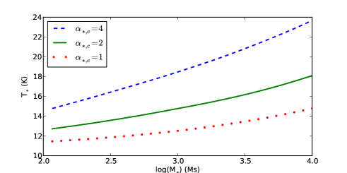
Figure 3: Mean gas temperature for various proto-cluster masses.

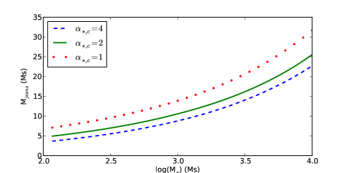
Figure 4: Jeans mass vs proto-cluster masses.

3.3.2 Temperature distribution within proto-clusters

As discussed in Hennebelle & Chabrier (2009, HC2009), the equation of state has a significant influence on the core mass function. Knowing the mean temperature only, does not appear to be sufficient, therefore. Instead one needs to know the complete equation of state, that is to say, how the temperature varies with the density within the proto-clusters. For that purpose, we compute the temperature at various densities, assuming that the turbulent heating $\Gamma_{\rm turb}$ and the gradient per km s^-1 used for the molecular cooling correspond to the mean conditions within proto-clusters of mass $M_{*}$. This means that we are assuming that both the heating and the cooling, only depend on the large scale conditions and do not vary locally.

Figure 5 shows the gas temperature as a function of density for various proto-cluster masses. For densities between $10^{3}$ and $\simeq 10^{6}$ cm^-3, the temperature decreases from about 20 to $\simeq 8$K, leading to an effective adiabatic exponent of about $\simeq 0.85-0.9$. At higher densities, the temperature increases slightly due to the influence of the dust. The minimum temperature is reached for $n\simeq 5-8\times 10^{5}$ cm^-3. This compares reasonably well with the temperature distributions displayed in Fig. 2 of Larson (1985). The proto-cluster mass does not have a drastic influence on the temperature distribution with variations of a few degrees only.

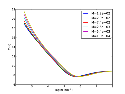
Figure 5: Temperature vs density for various proto-cluster masses.

3.4 Mass distribution: Hennebelle-Chabrier theory

In this section, we briefly describe the ideas and the formalism of the Hennebelle-Chabrier theory of star formation (HC2008, HC2009, HC2011) that is used in this manuscript to infer the IMF within clusters. In this theory the prestellar cores that eventually lead to protostars and then stars correspond to the turbulent density fluctuations that arise in a supersonic medium, which become sufficiently dense to be self-gravitating. These fluctuations are counted by using the formalism developed in cosmology by Press & Schechter (1974) although with a formulation close to the approach of Jedamzik (1995). Recently, Hopkins (2012) formulates the problem using the excursion set theory (e.g. Bond et al. 1991) formalism. He also extends the calculation by considering the whole galactic disk. His results regarding the small scale self-gravitating fluctuations (the last crossing barrier) are undistinguishable from the HC2008 result at small masses and only slightly different at high mass.

According to various simulations of hydrodynamic or MHD supersonic turbulence, the density PDF is well represented in both cases by a lognormal form,

$${\cal P}(\delta) = {1\over\sqrt{2\pi\sigma_{0}^{2}}}\exp\left(-{(\delta-\bar{\delta})^{2}\over 2\sigma_{0}^{2}}\right),\;\delta=\ln(\rho/\rho_{0}),$$ (30)

$$\bar{\delta} = -\sigma_{0}^{2}/2\;,\;\sigma_{0}^{2}=\ln(1+b^{2}{\cal M}^{2}),$$

where ${\cal M}$ is the Mach number, $b\simeq 0.5-1$ (Kritsuk et al. 2007, Audit & Hennebelle 2010, Federrath et al. 2010) and $\rho_{0}$ is the mean density.

The self-gravitating fluctuations are determined by identifying the structures of mass $M$ in the cloud’s random field of density fluctuations. These are gravitationally unstable at scale $R$, according to the virial theorem. This condition defines a scale-dependent (log)-density threshold, $\delta_{R}^{c}=\ln(\rho_{c}(R)/{\rho_{0}})$, or equivalently, a scale-dependent Jeans mass, $M_{R}^{c}$

$$M_{R}^{c}=a_{J}^{2/3}\left({(C_{s})^{2}\over G}R+{V_{0}^{2}\over 3\,G}\left({R\over 1{\rm pc}}\right)^{2\eta}R\right),$$ (31)

where $C_{s}$ is the sound speed, G the gravitational constant, $a_{J}$ a constant on order of unity while $V_{0}$ and $\eta$ determine the rms velocity,

$$\langle V_{\rm rms}^{2}\rangle=V_{0}^{2}\times\left({R\over 1{\rm pc}}\right)^{2\eta}.$$ (32)

Because a fluctuation of scale $R$ is replenished within a typical crossing time $\tau_{R}$, and is therefore replenished a number of time equal to $\tau^{0}_{ff}/(\phi_{t}\tau_{R,ff})$, where $\tau_{R,ff}=\tau_{R}/\phi_{t}$ is the freefall time at scale $R$ (see Appendix of HC2011), i.e. at density $\rho_{R}\sim M_{R}/(4\pi/3R^{3})$, HC2011 includes this condition into the formalism originally developed in HC2008. This yields for the number-density mass spectrum of gravitationally bound structures, ${\cal N}(M)=d(N/V)/dM$

$${\cal N}(M_{R})\simeq{{\rho_{0}}\over M_{R}}{dR\over dM_{R}}\times\left(-{d\delta_{R}\over dR}e^{\delta_{R}}({\tau^{0}_{ff}\over\tau_{R}}){\cal P}(\delta_{R})\right),$$ (33)

which is Eq. (6) of HC2011 and except for the time ratio ${\tau^{0}_{ff}\over\tau_{R}}$, is similar to Eq. (33) of HC2008. Note that we have dropped the second term which appears in Eq. (33) and which entails the derivative of the density PDF. For the strongly self-gravitating regimes that we are considering here, this approximation is well satisfied.

Equation (33) gives the mass spectrum that we are computing in the following. It depends on $M_{R}$ and $dM_{R}/dR$, which can be obtained from Eq. (31). To proceed, it is more convenient to normalize the expressions. After normalisation, Eq. (31) becomes

$$\widetilde{M}_{R}^{c}=M/M_{J}^{0}=\widetilde{R}\,\left(f(\rho)+{\cal M}^{2}_{*}\widetilde{R}^{2\eta}\right),$$

$$f(\rho)=f({\tilde{M_{R}^{c}}\over\tilde{R}^{3}})={C_{s}^{2}\over(C_{s}^{0})^{2}},$$ (34)

where $C_{s}^{0}=C_{s}(\rho_{0})$, $M_{J}^{0}$, $\lambda_{J}^{0}$ and ${\cal M}_{*}$ are given by

$$M_{J}^{0} = a_{J}\,{(C_{s}^{0})^{3}\over\sqrt{G^{3}\rho_{0}}}\approx 1.0\,\,a_{J}\,({T\over 10\,{\rm K}})^{3/2}\,({\mu\over 2.33})^{-1/2}\,$$ (35)

$$\times ({n_{0}\over 10^{4}\,{\rm cm}^{-3}})^{-1/2}\,{\rm M}_{\odot},$$

$$\lambda_{J}^{0} = \left({a_{J}\over C_{m}}\right)^{1/3}{(C_{s}^{0})\over\sqrt{G\rho_{0}}}\approx 0.1\,a_{J}^{1/3}\,({T\over 10\,{\rm K}})^{1/2}\,({\mu\over 2.33})^{-1/2}\,$$ (36)

$$\times ({n_{0}\over 10^{4}\,{\rm cm}^{-3}})^{-1/2}\,\,{\rm pc},$$

$${\cal M}_{*} = {1\over\sqrt{3}}{V_{0}\over C_{s}}\left({\lambda_{J}^{0}\over 1{\rm pc}}\right)^{\eta}$$ (37)

$$\simeq (0.8-1.0)\,\left({\lambda_{J}^{0}\over 0.1\,{\rm pc}}\right)^{\eta}\,\left({C_{s}\over 0.2\,{\rm km\,s}^{-1}}\right)^{-1},$$

$a_{J}$ and $C_{m}$ being dimensionless geometrical factors on the order of unity. Taking for example the standard definition of the Jeans mass, as the mass enclosed in a sphere of diameter equal to the Jeans length, we get $a_{J}=\pi^{5/2}/6$ while $C_{m}=4\pi/3$ (e.g. HC2009).

With Eqs. (30) and (33), we obtain

$${\cal N}(\widetilde{M}) = -{1\over\phi_{t}}{\rho_{0}\over M_{J}^{0}\widetilde{M}}\left({\widetilde{M}_{R}^{c}\over\widetilde{R}^{3}}\right)^{1/2}{d\widetilde{R}\over d\widetilde{M}_{R}^{c}}{d\delta_{R}^{c}\over d\widetilde{R}}$$ (38)

$$\times {1\over\sqrt{2\pi\sigma^{2}}}\exp\left(-{(\delta_{R}^{c})^{2}\over 2\sigma^{2}}+{\delta_{R}^{c}\over 2}-{\sigma^{2}\over 8}\right).$$

An important difference to the work of HC2009 is that the equation of state shown in Fig. 5 is not polytropic, but fully general. To obtain $d\tilde{M}_{R}^{c}/d\tilde{R}$, we must differentiate Eq. (34), which leads to (see Appendix of HC2009)

$${d\tilde{M}_{R}^{c}\over d\tilde{R}}={f({\tilde{M_{R}^{c}}\over\tilde{R}^{3}})-3{\tilde{M_{R}^{c}}\over\tilde{R}^{3}}f^{\prime}({\tilde{M_{R}^{c}}\over\tilde{R}^{3}})+(2\eta+1){\cal M}_{*}^{2}\tilde{R}^{2\eta}\over 1-{1\over\tilde{R}^{2}}f^{\prime}({\tilde{M_{R}^{c}}\over\tilde{R}^{3}})}.$$ (39)

With this last equation, all quantities appearing in Eq. (38) are known and the mass spectrum of the condensations can be computed. Note that $M_{R}$ must be computed numerically from Eq. (34).

4 Results: mass distribution of self-gravitating condensations in clusters

In this section we calculate the mass spectrum of the self-gravitating fluctuations and discuss its dependence on the various parameters.

4.1 Preliminary considerations

Before presenting the complete distribution, we start by discussing the position dependence of the distribution peak. For that purpose we make various simplifying assumptions.

4.1.1 Peak position: dependence on the Jeans mass and Mach number

Unlike what is often assumed in the literature, it is unlikely that the peak of the CMF/IMF solely depends on the Jeans mass. In particular, it likely depends on the Mach number because compressible turbulence creates high density regions where the Jeans mass is smaller. Indeed, in any turbulent medium, there is a distribution of Jeans masses rather than a single well-defined value. The peak position has been calculated by HC2008 who show (their Eq. 46 ) that $M_{\rm peak}=M_{J}^{0}/(1+b^{2}{\cal M}^{2})^{3/4}$ (note that in HC2008 $b$ stands for $b^{2}$ as different notations were used). However, as discussed above, time-dependence is not considered in HC2008 while it is taken into account in Eq. (38) through the term $1/\tau_{R}$. To calculate the peak position in this case, we proceed as in HC2008, that is to say we neglect the turbulent support (i.e. we set ${\cal M_{*}}=0$), which has little influence on the peak position. We also assume strict isothermality within the cluster, that is to say, we set $f=1$. As discussed in HC2009, the equation of state indeed has an influence on the peak position. However, as portrayed in Fig. 5, the deviation from the isothermal case is not very important with an effective adiabatic index of 0.85-0.9. Moreover, our goal here is more to discuss the dependence qualitatively rather than getting an accurate estimate, which is calulated later in the manuscript.

Assuming ${\cal M_{*}}=0$ and $f=1$, it is easy to take the derivative of Eq. (38) and to show that the maximum of ${\cal N}(\tilde{M})$ is reached for $\tilde{M}=1/(1+b^{2}{\cal M}^{2})$, which implies that the distribution peak is reached at

$$M_{\rm peak}={M_{J}^{0}\over 1+b^{2}{\cal M}^{2}}.$$ (40)

The difference to the expression presented in HC2008 comes from the fact that more small structures form when time dependence is taken into account since the small scale fluctuations are rejuvenated many times while the larger ones are still evolving.

Note that as already stressed, the peak position does not depend on the Jeans mass only, but also on the Mach number. For a typical $b^{2}$ of the order of $\simeq$0.5 (see Federrath et al. 2010) and a Mach number of about 5, we derive that the peak position is typically shifted by a factor of about 10 with respect to the mean Jeans mass.

4.1.2 Dependence of the peak position on the cluster mass

To estimate the peak position, we must therefore estimate the Jeans mass and the Mach number as a function of the cluster parameters. Since the Jeans mass is equal to $(\pi^{5/2}/6)C_{s}^{3}/\sqrt{\rho_{0}G}$, we obtain that

$$M_{\rm peak}\simeq{\pi^{5/2}\over 6}{C_{s}^{5}\over b^{2}G^{1/2}(\rho_{*})^{1/2}\sigma_{*}^{2}}.$$ (41)

To estimate the sound speed we must compute the mean temperature within the proto-cluster. For the sake of simplicity, we consider in this analytical estimate the turbulent heating $\Gamma_{turb}$ and the molecular cooling $\Lambda_{mol}$ given by Eqs. (21) and (24), respectively. Writing $\Gamma_{turb}=\Lambda_{mol}/n$, we obtain the temperature and thus the sound speed

$$C_{s}^{5} = \left({k\over m_{p}}\right)^{5/2}\left({6\over 5}{Gm_{p}\over 1\,{\rm pc}}\right)^{5/(2d)}\left({Q_{0}(M_{*}^{0})^{0.75}\over\Lambda_{0}n^{c}}\right)^{5/(2d)}$$ (42)

$$\times \left({R_{*}\over 1\,{\rm pc}}\right)^{5/(4d)}.$$

On the other hand, with Eqs. (18)-(19), we derive

$${1\over\sqrt{\rho_{*}}\sigma^{2}}={\sqrt{4\pi/3(1\,{\rm pc})^{3}}\over(2\sqrt{3}G)^{2/3}}{1\over Q_{0}^{2/3}(M_{*}^{0})^{1/2}}\left({R_{*}\over 1{\rm pc}}\right)^{-1/2}.$$ (43)

This leads to

$$M_{\rm peak} \simeq K{Q_{0}^{5/(2d)-2/3}(M_{*}^{0})^{15/(8d)-1/2}\over\Lambda_{0}^{5/(2d)}n_{c}^{5c/(2d)}}\left({R_{*}\over 1\,pc}\right)^{5/(4d)-1/2},$$

$$K = {\pi^{5/2}\over 6}{1\over G^{1/2}b^{2}}\left({k\over m_{p}}\right)^{5/2}\left({6\over 5}{Gm_{p}\over 1\,{\rm pc}}\right)^{5/(2d)}$$ (44)

$$\times {\sqrt{4\pi/3(1\,{\rm pc})^{3}}\over(2\sqrt{3}G)^{2/3}}.$$

As already mentioned, typical values of $d$ are 2-2.5 while $c$ is typically low and close to zero. Ignoring the dependence on $n^{c}$, the peak position consequently has a weak dependence on the cluster radius, which typically depends on $R$ as $R_{*}^{1/8-0}$. This is the result of partial compensation of the sound speed, the density and the velocity dispersion. Thus we can conclude that in the regime where turbulent heating dominates over the cosmic ray heating, the initial mass function is expected to weakly depend on the cluster masses. According to our estimate, this is the case for large mass clusters, i.e. with masses above $\simeq 10^{3}M_{\odot}$. Note that it should be kept in mind that in this analysis, isothermality is assumed, which is also a simplification.

Before solving for the whole mass spectrum obtained with a complete equation of state, it is worth computing the dependence of $M_{\rm peak}\simeq M_{J}^{0}/(1+b^{2}{\cal M}^{2})$ on the proto-cluster mass and on $Q_{0}\propto\alpha_{*,c}^{0.75}$, the parent clump over proto-cluster mass ratio using the complete thermal balance stated by Eq. (29) rather than the simplified approach used above. Figure (6) portrays the value of $M_{peak}=M_{J}^{0}/(1+b^{2}{\cal M}^{2})$ as a function of the proto-cluster mass for three values of $\alpha_{*,c}$ and $b=0.6$. This last value corresponds to a mixture of solenoidal and compressive modes (Federrath et al. 2008). The trends are similar to what has been inferred from Eq. (29), that is to say, the peak position weakly depends on the proto-cluster mass and more strongly on the accretion rate controlled by $\alpha_{*,c}$. However, it is remarkable that for proto-clusters whose masses are between $10^{2}$ and $10^{4}$ M_⊙, and within the ranges $\alpha_{*,c}=[1,4]$, which encompasses most of the data points reported in Fig. 2, the peak position varies by a factor of only 3 and only 2 for $M_{c}$ between 10³ and 10⁴ M_⊙.

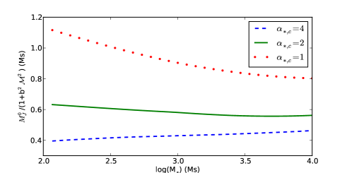
Figure 6: Expected position of the CMF peak as a function of the proto-cluster mass for 3 values of the ratio of parent clump over proto-cluster mass ratio, $\alpha_{*,c}$.

4.2 Fiducial parameters

We now present the complete mass spectrum obtained by iteratively solving Eq. (34) and computing Eqs. (38) and (39) using the temperature distribution obtained in section 3.3.2 and portrayed in Fig. 5. Because the latter is not analytical, it is difficult to take its derivative as required by Eq. (39). Thus for this purpose we first obtain a fit of the temperature using a high order polynomial.

Figure 7: Mass spectra for various cluster masses and the fiducial value $\alpha_{*,c}=2$. The dots represents the Chabrier IMF. The two lines represents the distribution $M^{-2}$ and $M^{-2.3}$. The upper panel displays the mass distribution obtained with Eq. (38) while the lower panel shows this mass distribution convolved by a Gaussian of dispersion $\sigma=M/2$.

Upper panel of Fig. 7 portrays the resulting mass spectra for various cluster masses as labeled in the figure. The dots represent the Chabrier IMF (Chabrier 2003) shifted by a factor of about 2. Indeed, since we compute the mass function of self-gravitating condensations, this shift is necessary to account for the observed shift between the CMF and the IMF (e.g. Alves et al. 2007, André et al. 2010) and for the theoretical estimate for the core-to-star efficiency (Matzner & McKee 2000, Ciardi & Hennebelle 2010). Because we do not consider any cluster mass distribution and efficacity problem here, we set the distribution maximum to 1. This allows us to compare the shape of the various distributions more easily.

Various points are worth discussing. First of all, the distributions all agree with the Salpeter and Chabrier IMF at high masses. As discussed in HC2008, this is because the high mass part is essentially due to the turbulent support, which does not change much in this regime. Moreover, the high mass part of the distribution tends to slowly depend on the parameters that control the turbulence, namely ${\cal M}$ and ${\cal M}_{*}$. Second, the peak position varies by about a factor 2 as the proto-cluster mass changes from $\simeq 10^{2}M_{\odot}$ to about $10^{4}M_{\odot}$ while the distributions corresponding to $M_{*}=10^{3}$ and $10^{4}$ $M_{\odot}$ are nearly indistinguishable. This weak variation is, as discussed in the previous section, a consequence of various quantities compensating each other. Third, the position of the peak itself is close to the peak of the Chabrier IMF shifted by a factor of 2.

4.3 Link between the CMF and the IMF

An important question regarding the mass distribution is the link between the IMF and the CMF, which is not expected to be as simple as a unique efficiency (e.g. Alves et al. 2007, Goodwin et al. 2008) on the order of 2-3. It is instead expected that the two distributions are correlated with some dispersion because the initial mass and velocity distributions within the cores vary from one core to another, therefore leading to different evolutions. In other words, the virial theorem is not representing the problem in its full complexity and the initial conditions and the boundary conditions (which enter through the surface terms, see e.g. Dib et al. 2007) influence the mass of the objects that form within the collapsing cores. Indeed, Smith et al. (2008) have shown that in hydrodynamical simulations, the correlation between the mass of the sink particles and the cores in which they are embedded is very good during the first freefall times and becomes less tight after $\simeq 5$ freefall times. This is because initially the sink particles are accreting the mass of the parent core. As time evolves, the material that falls onto the sinks comes for further away and is less and less correlated to the initial mass reservoir. More quantitatively, Chabrier & Hennebelle (2010) have shown that in the simulations of Smith et al. (2008), the correlation between the CMF and the sink particles mass function, which is likely representing the IMF, can reasonably be reproduced at intermediate time (say 3-5 freefall time) by a Gaussian distribution with a width, $\sigma$, on the order of $M/3-M/2$. To take this into account, we have convolved the mass distribution portrayed in the upper panel of Fig. 7 with a Gaussian distribution of width $\sigma_{conv}=M/2$.

$${dN\over dM}_{conv}(M)={\int_{0}^{\infty}{dN\over dM}(M^{\prime})\exp\left({-(M-M^{\prime})^{2}\over 2\sigma_{conv}^{2}}\right)dM^{\prime}\over\int_{0}^{\infty}\exp\left({-(M-M^{\prime})^{2}\over 2\sigma_{conv}^{2}}\right)dM^{\prime}}.$$ (45)

Note that in principle, since the efficiency of the accretion is lower than one, the distribution should be shifted toward smaller masses (e.g. Alves et al. 2007, André et al. 2010). In practice, to facilitate the comparison with $dN/dM$, we have not shifted it here.

As expected, the distribution $dN/dM_{conv}$ is slightly broader than the distribution $dN/dM$ in particular at low masses whereas, the high mass part and the peak position are almost unchanged. This effect could therefore in particular contribute to the formation of low mass brown dwarfs. To clarify, because some cores are marginally bound, for example because their velocity field is initially globally diverging, few objects significantly less massive than the parent core mass form, most of the envelope being then dispersed in the surrounding ISM.

To summarize, for an accretion rate that allows one to reproduce the mass-size relation of clusters, we self-consistently predict a distribution of self-gravitating structures that $i)$ is very close to the field IMF inferred by Chabrier (2003), $ii)$ is almost independent on the cluster mass for gas masses larger than $10^{3}M_{\odot}$. We stress that if more variability is expected for low mass clusters, it is very difficult to infer any reliable statistics and thus no data are available in this regime.

4.4 Dependence on the accretion rate

Because the accretion rate onto the proto-clusters of a given mass is likely varying, as suggested by Fig. 2, we explore the effect of this parameter on the whole mass spectrum. As anticipated in Fig. 6, it has some influence on the peak position. As discussed in section 2.1, we use the parent clump mass over proto-cluster mass ratio to quantify the accretion rate following Eqs. (2.1.3)-(4) and we select the two values $\alpha_{*,c}=1$ and 4, which as shown by Fig. 2 encompass almost all points of the observational distribution.

The mass distributions obtained for $\alpha_{*,c}=1$ and 4 are displayed in upper and lower panels of Fig. 8, respectively, which shows that the trends inferred in Fig. 6 are well confirmed. The mass distribution is shifted toward larger masses for a lower accretion rate ($\alpha_{*,c}=1$) and toward smaller masses for a higher accretion rate ($\alpha_{*,c}=4$). Apart from this, the general behaviour is almost identical to the fiducial case $\alpha_{*,c}=2$, that is to say, the distributions weakly depend on the proto-cluster gas masses for $M_{*}\simeq 10^{3}-10^{4}$ M_⊙ and the high mass part is always close to the Salpeter IMF.

Importantly enough, we note that within the range $1<\alpha_{*,c}<4$ the variation of the mass spectrum with the accretion rate remains limited to a factor of about 2 almost everywhere, especially for the proto-clusters, whose mass of gas is between 10³ and $10^{4}$ M_⊙.

Figure 8: Mass spectra for various cluster masses, upper panel $\alpha_{*,c}=1$, lower panel $\alpha_{*,c}=4$. As in Fig. 7 the dots represents the Chabrier IMF. The two lines represents the distribution $M^{-2}$ and $M^{-2.3}$.

4.5 Dependence on cosmic rays and radiation

Another source of possible variability are the heating sources, namely cosmic rays and interstellar radiation field, which heat the gas and the dust respectively. In this section, we investigate the dependence of the CMF on these parameters. Indeed, both are likely varying as one approaches a supernova remnant or a massive star for example.

4.5.1 Dependence on cosmic rays

Figure 9: Same as Fig. 7 for the fiducial value $\alpha_{*,c}=2$ but for two values of cosmic rays. The upper panel shows cosmic ray heating twice lower than the fiducial value while the lower panel shows cosmic ray heating three times higher.

Figure 9 shows the mass distribution for two values of cosmic rays heating, namely half (upper panel) and three times the fiducial value stated by Eq. (23). As can be seen from a comparison with the upper panel of Fig. 7, cosmic ray heating has an impact on the mass distribution that is only moderate. For most of the distribution, the variations are typically less than a factor two.

4.5.2 Dependence on radiation

Figure 10: Same as Fig. 7 for the fiducial value $\alpha_{*,c}=2$ but for two values of the radiation field. The upper panel shows an interstellar radiation field equal to half the canonical values while the lower panel shows a radiation field twice as high.

When increasing the interstellar radiative fields, the various components must be distinguished since they have a different physical origin. For simplicity we multiply all components by the same factor except for the cmb component, which is kept constant. Figure 10 shows the mass distribution for two values of interstellar radiation field, namely half (upper panel) and twice the fiducial value. The departure from the mass distribution displayed in Fig. 7 is even smaller than for the cosmic rays. This is because the radiation field is modifying the dust temperature, which has only a weak impact on the mass distribution because, as discussed above, the effective $\gamma$ at low and high density are about 0.85-9 and 1, respectively (see Fig. 5).

4.6 Discussion

One of the central questions regarding the IMF is that of its apparent universality, that is to say, its apparent lack of variations in the different determinations that have been made so far (e.g. Moraux et al. 2007, Bastian et al. 2010). The various estimates in open clusters and young clusters lead to some variability on the IMF parameters, in particular on the characteristic mass, or peak position, but as pointed out by de Marci et al. (2010) dynamical evolution is a plausible explanation to account for the strongest variations. There is a possible variation independent of the cluster dynamical evolution, however, as can be seen for example in Fig. 3 (left panel) of Bastian et al. (2010) and in Fig. 2 of de Marci et al. (2010), which shows that at a given dynamical age, the value of $m_{c}$ typically varies over a factor of about 2. It is worth stressing that a possible deficiency of brown dwarfs is observed in Taurus (e.g. Guieu et al. 2006, Luhman et al. 2009, Bastian et al. 2010) while a possible excess (factor of about 2) may have been observed in $\sigma$ Ori and Upper Sco (e.g. Caballero et al. 2007). These variations need to be confirmed, however. It is clearly difficult, at this stage, to give a definite conclusion.

On the other hand, the results obtained in this paper can be broadly summarized as follows: $i)$ the high mass part of the IMF is robust to all variations explored in this paper (higher accretion rate could lead to some flattening and shift the peak toward smaller masses), $ii)$ the low mass part varies with the mass of the cluster and the accretion rate by a factor of about 2 in the range we explored. The variation with the cluster mass in the range 500-10⁴ $M_{\odot}$ is very limited, typically less than a factor 2 (see the four more massive cases displayed in Fig. 7) and thus account well for the lack of variability since as displayed in table 1 of de Marci et al. (2010), most of the clusters that we studied have a mass of stars that is comparable to or greater than, $10^{2}$ $M_{\odot}$. This in turn corresponds to a mass of gas about five times larger, assuming an efficiency of 20%. The variation of the mass function with the accretion rate, i.e. with $\alpha_{*,c}$, is more significant but remains compatible with the range of values that we inferred from the comparison with the data from Lada & Lada (2003), that is to say a factor of about 2 for the accretion rate (at fixed mass) and a factor of about 2-3 on the low mass part of the distribution (with much stronger variations for the very low mass objects).

5 Conclusion

We have developed an analytical model that successfully reproduces the mass-size relation of embedded clusters. It is based on the continuous accretion of gas that drives the turbulence which in turn resists the gravitational contraction and determines the cluster radius. Comparing the mass-size relation with the available data of embedded clusters, we showed that they can be well fitted by employing an accretion rate that is entirely reasonable and close to the rate that can be inferred using Larson relations. Moreover, the variation of this parameter needed to reproduce the dispersion of observational data is moderate being equal to a factor of about 2. Eventually, the turbulent energy dissipates and heats the gas. Performing a thermal balance, we calculated the temperature distribution within the cluster and applied a time-dependent version of the HC2008 theory to obtain the mass spectrum of self-gravitating condensations. The peak position and more generally the whole mass spectrum is inferred from a large domain of proto-cluster masses. We found that for gas masses between 500 to $10^{4}$ $M_{\odot}$ corresponding to a mass of stars roughly 5 times smaller, the mass spectrum of self-gravitating condensations does not vary significantly. The mass spectrum varies more significantly with the accretion rate, but given the range of accretion rate deduced from the observational comparison, they remain compatible with the available determination of the IMF in the Galaxy.

6 Acknowledgments

We thank the anonymous referee for comments that have significantly improved the original manuscript. PH warmly thanks Gilles Chabrier, Jérôme Bouvier and Ralf Klessen for many related stimulating discussions. He also thanks Eugene Chiang and Chris Matzner for stimulating discussions on cluster formation during the ISIMA summer school hosted by the KIAA in Beijing.

Appendix A Virial theorem for an accreting system

The virial theorem is derived in many textbooks (e.g. Shu 1992, Kulsrud 2005, Lequeux 2005) and does not need to be presented. However, it is most of the time assumed that the system has a constant mass, i.e. is not accreting. Here we derive its expression for a system accreting at a rate $\dot{M}$ (see also Goldbaum et al. 2011). That is to say, at radius $R(t)$, gas at density $\rho_{inf}$ is falling into the cluster with a velocity $v_{inf}$.

We start as usual by multiplying the momentum conservation equation by the vector position ${\bf r}$ and integrating over the volume. The right-hand side of the momentum conservation equation is equal to the sum of the forces, namely thermal pressure and gravity (and Lorentz force when the magnetic field is considered). It can be rewritten in the unmagnetized case as $2E_{therm}-3P_{therm}V+E_{g}$, where $E_{therm}$ is the thermal energy, $P_{therm}$ is the thermal pressure, $V$ is the volume and $E_{g}$ the gravitational energy. The left-hand side is given by $\int\rho d_{t}v_{i}r_{i}dV$. Integrating this expression by part, we have

$$\int\rho d_{t}v_{i}r_{i}dV = \int\rho d_{t}(v_{i}r_{i})dV-\int\rho v_{i}^{2}dV,$$

$$= \int\rho\partial_{t}(v_{i}r_{i})dV+\int\rho{\bf v.grad}(v_{i}r_{i})dV$$

$$-\int\rho v_{i}^{2}dV,$$

$$= \partial_{t}(\int\rho v_{i}r_{i}dV)+\int{\rm div}(\rho v_{i}r_{i}{\bf v})dV$$

$$-\int\rho v_{i}^{2}dV,$$

$$= \partial_{t}(\int\rho d_{t}(r_{i}^{2})/2dV)+\int\rho v_{i}r_{i}{\bf v}{\bf dS}$$

$$-\int\rho v_{i}^{2}dV,$$

where we used the continuity equation $\partial_{t}\rho+{\rm div}(\rho{\bf v})=0$ to cancel some of the terms.

Let us consider now the first term which appear in the right-hand side. We can write

$$\int\rho v_{i}r_{i}dV = \int\rho d_{t}(r_{i}^{2})/2dV=\int\rho\partial_{t}(r_{i}^{2})/2dV$$

$$+\int\rho{\bf v.grad}(r_{i}^{2}/2)dV,$$

$$= \int\partial_{t}(\rho r_{i}^{2}/2)dV+\int{\rm div}(\rho r_{i}^{2}{\bf v})/2dV,$$

$$= \partial_{t}(\int\rho r_{i}^{2}/2dV)+\int\rho r_{i}^{2}/2{\bf v.dS}.$$

Thus Eqs. (A) and (A) lead to

$$\int\rho d_{t}v_{i}r_{i}dV = \partial_{t}^{2}(\int\rho r_{i}^{2}/2dV)+\partial_{t}(\int\rho r_{i}^{2}/2{\bf v.dS})$$

$$+\int\rho v_{i}r_{i}{\bf v}{\bf dS}-\int\rho v_{i}^{2}dV,$$

$$= {1/2}\partial^{2}_{t^{2}}I-\partial_{t}(\rho v_{inf}R^{2}S)$$

$$+\rho_{inf}v_{inf}^{2}RS-2E_{c},$$

$$= {1/2}\partial^{2}_{t^{2}}I-{1\over 2}\partial_{t}(\dot{M})R^{2}-{1\over 2}\dot{M}^{2}\partial_{M}R^{2}$$

$$+3P_{ram}V-2E_{c},$$

where $I=\int\rho r_{i}^{2}dV$, $\dot{M}=\rho_{inf}v_{inf}S$ and $P_{ram}=\rho_{inf}v_{inf}^{2}$. Note that the minus sign in the second and third terms of the right-hand side, are due to the fact that as the gas is infalling, $v_{inf}<0$ and thus ${\bf v.dS}<0$.

The complete expression for the virial theorem is thus

$${1/2}\partial^{2}_{t^{2}}I = {1\over 2}\partial_{t}(\dot{M})R^{2}+{1\over 2}\dot{M}^{2}\partial_{M}R^{2}-3(P_{ram}+P_{therm})V$$ (49)

$$+2E_{c}+2E_{therm}+E_{g}.$$

Assuming stationarity and neglecting thermal support and thermal pressure, we derive

$${1\over 2}\dot{M}^{2}\partial_{M}R^{2}-3P_{ram}V+2E_{c}+E_{g}=0,$$ (50)

which is the equation used in this paper.

Appendix B Gravitational energy released by accretion

We calculate here the gravitational energy that is released when a particle of gas is accreted onto the proto-cluster. For that purpose, we assume the following. First, the accreted particles that enter the proto-cluster, will on average be distributed uniformly within the cluster, second, we assume that the gravitational energy inside the cluster is produced by a uniform distribution of matter, i.e. we neglect the influence of any local density fluctuations.

Under these assumptions the gravitational force inside the proto-cluster is $-G4\pi/3\rho_{*}r$ and the gravitational potential is thus $G2\pi/3(r^{2}-3R_{*}^{2})$. Since the gravitational potential outside the cluster is $-GM_{*}/r$, it can easily be checked that the gravitational potential is continuous throughout the cluster boundary, i.e. at $r=R_{*}$. Therefore we get that the mean specific gravitational energy, $e_{g}$, of a particle that falls into the proto-cluster is

$$e_{g}=-\int_{0}^{R_{*}}{G2\pi\rho_{*}\over 3}(3R_{*}^{2}-r^{2})f(r)dr=-{6\over 5}{GM_{*}\over R_{*}},$$ (51)

where $f(r)dr=3r^{2}dr/R_{*}^{3}$ is the fraction of particles located between $r$ and $r+dr$.

Thus the total accretion energy rate is

$$\dot{E}_{\rm ext}={6\over 5}{GM_{*}\dot{M}\over R_{*}}.$$ (52)

References

- (1) Allen, L., Megeath, S., Gutermuth, R. et al. 2007, prpl.conf, 361
- (2) André, P., Men’shchikov, A., Bontemps, S. et al. 2010, A&A, 518L, 102
- (3) Audit, E., Hennebelle, P., 2010, A&A, 511, 76
- (4) Banerjee, R., Vázquez-Semadeni, E., Hennebelle, P., Klessen, R., 2009, MNRAS, 398, 1082
- (5) Bastian, N., Covey, K., Meyer, M., 2010, ARA&A, 48, 339
- (6) Bate, M., 2009, MNRAS, 392, 1363
- (7) Black, J., 1994, ASPC, 58, 355
- (8) Bonnell, I., Bate, M., Clarke, C., 2006, MNRAS, 368, 1296
- Bond (1991) Bond, J., Cole, S., Efstathiou, G., Kaiser, N., 1991, ApJ, 379, 440
- (10) Bondi, H., 1952, MNRAS, 112, 195
- (11) Bressert, E., Bastian, N., Gutermuth, R., Megeath, S., Allen, L., et al. 2010, MNRAS, 409L, 54
- (12) Burke, J., Hollenbach, D., 1983, ApJ, 265, 223
- (13) Caballero, J., et al. 2007, A&A, 470, 903
- (14) Capellari, M., McDermid, R., Alatalo, K., et al., 2012 Natur, 484, 485
- (15) Chabrier, G., 2003, PASP, 115, 763
- CH (2010) Chabrier, G., Hennebelle, P., 2010, ApJ, 725L, 79
- ciardi hennebelle (2010) Ciardi, A., Hennebelle, P., 2010, MNRAS, 409L, 39
- (18) de Marchi, G., Paresce, F., Portegies Zwart, S., 2010, ApJ, 718, 105
- dib (2007) Dib, S., Kim, D., Vázquez-Semadeni, E., Burkert, A., Shadmehri, M., 2007, ApJ, 661, 262
- dib (2007) Dib, S., Kim, D., Shadmehri, M., 2007, MNRAS, 381L, 40
- dib (2010) Dib, S., Shadmehri, M., Padoan, P., Maheswar, G., Ohja, D., Khajenabi, F., 2010, MNRAS, 398, 401
- (22) Dib, S., Piau, L., Mohanty, S., Braine, J., 2011, MNRAS, 415, 3439
- elmegreen (2008) Elmegreen, B., Klessen, R., Wilson, C., 2008, ApJ, 681, 365
- (24) Falgarone, E.; Hily-Blant, P.; Levrier, F.; 2004, Ap&SS, 292, 285
- (25) Falgarone, E., Hily-Blant, P., Pety, J., 2009, A&A, 417, 243
- (26) Federrath, C., Klessen, R., Schmidt, W., 2008, ApJ, 688L, 79
- (27) Federrath, C., Roman-Duval, J., Klessen, R., Schmidt, W., MacLow, M.-M., 2010, A&A, 512, 81
- (28) Goldbaum, N., Krumholz, M., Matzner, C., McKee, C., 2011, ApJ, 738, 101
- (29) Guieu, S., Dougados, C., Monin, J.-L., Magnier, E., Martin, E., 2006, A&A, 446, 485
- (30) Goldsmith, P., 2001, ApJ, 557, 736
- (31) Goodwin, S., Nutter, D., Kroupa, P., Ward-Thompso, D., Whitworth, A., 2008, A&A, 477, 823
- Hennebelle & Audit (2007) Hennebelle, P., Audit, E., 2007, A&A, 465, 431
- Hennebelle & Chabrier (2008) Hennebelle, P., Chabrier, G., 2008, ApJ, 684, 395 (HC2008)
- Hennebelle & Chabrier (2009) Hennebelle, P., Chabrier, G., 2009, ApJ, 702, 1428(HC2009)
- Hennebelle & Chabrier (2011) Hennebelle, P., Chabrier, G., 2011, ApJ, 743L, 29 (HC2011)
- (36) Hopkins, P., 2012, MNRAS, 423, 2037
- jappsen (2005) Jappsen, A., Klessen, R., Larson, R., Li, Y., Mac Low,M.-M., 2005, A&A, 435, 611
- Jedamzik (1995) Jedamzik, K., 1995, ApJ, 448, 1
- (39) Juvela, M., Padoan, P., Nordlund, A., 2001, ApJ, 563, 853
- Kim & Ryu (2005) Kim, J., Ryu, D., 2005, ApJ, 630, L45
- (41) Klessen, R., Hennebelle, P., 2010, A&A, 520, 17
- Kritsuk (2007) Kritsuk, A., Norman, M., Padoan, P., Wagner, R., 2007, ApJ, 665, 416
- Kroupa (2002) Kroupa, P., 2002, Science, 295, 82
- krumholz (05) Krumholz, M., McKee, C., Klein, R., 2005, ApJ, 618, 757
- krumholz (11) Krumholz, M., 2011, ApJ, 745, 69
- krumholz (12) Krumholz, M., Klein, R., McKee, C., 2012, ApJ, 754, 71
- (47) Kulsrud, R., 2005, ppfa.book
- (48) Lada, C., Lada, E., 2003, ARA&A, 41, 57
- Larson (1981) Larson, R., 1981, MNRAS, 194, 809
- Larson (1985) Larson, R., 1985, MNRAS, 214, 379
- (51) Lequeux, J. 2005, in The interstellar medium, J. Lequeux (ed), EDP Sciences (Berlin: Springer)
- (52) Luhman, K., Mamajek, E., Allen, P., Cruz, K., 2009, ApJ, 703, 399
- (53) Matzner, C.D. & McKee, C., 2000, ApJ, 545, 364
- (54) Moreau, E., Bouvier, J., Stauffer, J., Barrado y Navascués, D., Cuillandre, J.-C., 2007, A&A, 471, 499
- (55) Murray, N., 2009, ApJ, 691, 946
- (56) Neufeld, D., Lepp, S., Melnick, G., 1995, ApJS, 100, 132
- (57) Ossenkopf, V., Henning, T., 1994, A&A, 291, 943
- Padoan & Nordlund (1997) Padoan, P., Nordlund, A., Jones, B., 1997, MNRAS, 288, 145
- (59) Passot, T., Vázquez-Semadeni, E., 1998, Phys. Rev. E, 58, 4501
- Press & Schechter (1974) Press, W., Schechter, P., 1974, ApJ, 187, 425
- Salpeter (1955) Salpeter, E., 1955,ApJ, 121, 161
- (62) Schmidt, W., Federrath, C., Hupp, M., Kern, S., Niemeyer, J., 2009, A&A, 494, 127
- (63) Schmidt, W., Kern, S., Federrath C., Klessen, R., 2010, A&A, 516, 25
- (64) Shu, F., 1992, pavi.book
- (65) Smith, R., Clark, P., Bonnell, I, 2008, MNRAS, 391, 1091
- Vazquez-Semadeni (94) Vázquez-Semadeni, E., 1994, ApJ, 423, 681
- Zucconi (2001) Zucconi, A., Walmsley, C., Galli, D., A&A, 376, 650