Ferrimagnetism of the Heisenberg Models on the Quasi-One-Dimensional Kagome Strip Lattices

Abstract

We study the ground-state properties of the $S=1/2$ Heisenberg models on the quasi-one-dimensional kagome strip lattices by the exact diagonalization and density matrix renormalization group methods. The models with two different strip widths share the same lattice structure in their inner part with the spatially anisotropic two-dimensional kagome lattice. When there is no magnetic frustration, the well-known Lieb-Mattis ferrimagnetic state is realized in both models. When the strength of magnetic frustration is increased, on the other hand, the Lieb-Mattis-type ferrimagnetism is collapsed. We find that there exists a non-Lieb-Mattis ferrimagnetic state between the Lieb-Mattis ferrimagnetic state and the nonmagnetic ground state. The local magnetization clearly shows an incommensurate modulation with long-distance periodicity in the non-Lieb-Mattis ferrimagnetic state. The intermediate non-Lieb-Mattis ferrimagnetic state occurs irrespective of strip width, which suggests that the intermediate phase of the two-dimensional kagome lattice is also the non-Lieb-Mattis-type ferrimagnetism.

I Introduction

Ferrimagnetism is a fundamental phenomenon in the field of magnetism. The simplest case of the conventional ferrimagnetism is the ground state of the mixed spin chain. For example, there is an ($s$, $S$)=(1/2, 1) mixed spin chain with a nearest-neighbor antiferromagnetic (AF) isotropic interaction. In this system, the so-called Lieb-Mattis (LM)-type ferrimagnetismLieb ; Marshall ; Takano ; Okamoto ; Tonegawa ; Sakai is realized in the ground state because two different spins are arranged alternately in a line owing to the AF interaction. Since this type of ferrimagnetism has been studied extensively, the magnetic properties and the occurrence mechanism of the LM ferrimagnetism are well known. In particular, the ferrimagnetism in the quantum Heisenberg spin model on the bipartite lattice without frustration is well understood within the Marshall-Lieb-Mattis (MLM) theoremLieb ; Marshall . In the LM ferrimagnetic ground state, the spontaneous magnetization occurs and the magnitude is fixed to a simple fraction of the saturated magnetization.

In recent years, a new type of ferrimagnetism, which is clearly different from LM ferrimagnetism, has been found in the ground state of several one-dimensional frustrated Heisenberg spin systemsPF1 ; PF2 ; PF3 ; PF4 ; PF5 ; Shimokawa ; Shimokawa2 . The spontaneous magnetization in this new type of ferrimagnetism changes gradually with respect to the strength of frustration. The incommensurate modulation with long-distance periodicity in local magnetizations is also a characteristic behavior of the new type of ferrimagnetism. Hereafter, we call the new type of ferrimagnetism the non-Lieb-Mattis (NLM) type. The mechanism of the occurrence of the NLM ferrimagnetism has not yet been clarified.

On the other hand, some candidates of the NLM ferrimagnetism among the two-dimensional (2D) systems, for example, the mixed-spin $J_{1}$-$J_{2}$ Heisenberg model on the square lattice2D-candidate1 and the $S=1/2$ Heisenberg model on the Union Jack lattice2D-candidate2 , were reported. These 2D frustrated systems have the intermediate ground state, namely, the “canted state”, in which the spontaneous magnetization is changed when the inner interaction of the system is varied. It has not been, however, determined whether the incommensurate modulation with long-distance periodicity exists in the local magnetization of the canted state owing to the difficulty of treating these 2D frustrated systems numerically and theoretically. Therefore, the relationships between the canted states of these 2D frustrated systems and the NLM ferrimagnetic state are still unclear.

Under these circumstances, recently, another candidate of the NLM ferrimagnetism among the 2D systems was reported in ref. References in which the $S=1/2$ Heisenberg model on the spatially anisotropic kagome lattice depicted in Fig. 1(a) was studied. A region of the intermediate-magnetization states is observed between the LM ferrimagnetism that is rigorously proved by the MLM theoremLieb ; Marshall and the nonmagnetic state of the spatially isotropic kagome-lattice antiferromagnet in the absence of magnetic fieldLecheminant ; Waldtmann ; Hida_kagome ; Cabra ; Honecker0 ; Honecker1 ; Cepas ; Spin_gap_Sindzingre ; HN_Sakai2010 ; Sakai_HN_PRBR ; HN_Sakai2011 . The local magnetization in the intermediate state of the kagome lattice was investigated by the exact diagonalization method, and it was reported that the local magnetization greatly depends on the position of the sites, although it is difficult to determine clearly whether the incommensurate modulation with long-distance periodicity is present. This result leads to the high expectation that the intermediate state of the spatially anisotropic kagome lattice is the NLM ferrimagnetic state. Additional research is desirable to conclude that the intermediate state of this 2D system is the NLM ferrimagnetism.

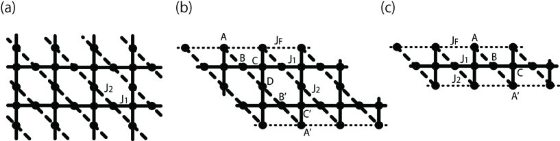
Figure 1: Structures of the lattices: the spatially anisotropic kagome lattice (a) and the quasi-one-dimensional kagome strip lattices (b) and (c) with different widths. An $S=1/2$ spin is located at each site denoted by a black circle. Antiferromagnetic bonds $J_{1}$ (bold straight line) and $J_{2}$ (dashed line), and ferromagnetic bond $J_{\rm F}$ (dotted line). The sublattices in a unit cell of lattice (b) are represented by A, ${\rm A}^{\prime}$, B, ${\rm B}^{\prime}$, C, ${\rm C}^{\prime}$, and D. The sublattices in a unit cell of lattice (c) are represented by A, ${\rm A}^{\prime}$, B, and C.

In this paper, we study the ground-state properties of the $S=1/2$ Heisenberg models on the quasi-one-dimensional (Q1D) kagome strip lattices depicted in Figs. 1(b) and 1(c) instead of the 2D lattice depicted in Fig. 1(a). Note that the inner parts of the lattices in Figs. 1(b) and 1(c) are common to a part of the 2D lattice in Fig. 1(a). We also note that the lattice shapes of strips in the present study are different from some kagome strips (chains) studied in refs. References-References, where the nontrivial properties of kagome antiferromagnets were reported.

According to the study in ref. References, it was already known that the NLM ferrimagnetism is realized in the ground state of the kagome strip lattice in Fig. 1(c). In the present study, we show that both the lattice in Fig. 1(c) and the lattice in Fig. 1(b) reveal the NLM ferrimagnetism in the ground state. Note also that the lattice shape at the edge under the open boundary condition depicted in Fig. 1(c) is different from that in ref. References [see Fig. 1(b) in ref. References]. Thus, one can recognize that the results of the strip lattice with small width are irrespective of boundary conditions. We also present clearly the existence of the incommensurate modulation with long-distance periodicity in the local magnetizations of both models in Figs. 1(b) and 1(c). Our numerical calculations suggest that the intermediate state of the 2D lattice in Fig. 1(a) is the NLM ferrimagnetism.

This paper is organized as follows. In §2, we first present our numerical calculation methods. In §3, we show the ground-state properties of the lattice depicted in Fig. 1(c) in finite-size clusters. In §4, we show the ground-state properties of the lattice depicted in Fig. 1(b). Sections 5 and 6 are devoted to discussion and summary, respectively.

II Numerical Methods

We employ two reliable numerical methods: the exact diagonalization (ED) method and the density matrix renormalization group (DMRG) methodDMRG1 ; DMRG2 .

The ED method is used to obtain precise physical quantities of finite-size clusters. This method does not suffer from the limitation of the cluster shape. It is applicable even to systems with frustration, in contrast to the quantum Monte Carlo (QMC) method coming across the so-called negative-sign problem for systems with frustration. The disadvantage of the ED method is the limitation that available system sizes are very small. Thus, we should pay careful attention to finite-size effects in quantities obtained by this method.

On the other hand, the DMRG method is very powerful when a system is (quasi-)one-dimensional under the open boundary condition. The method can treat much larger systems than the ED method. Note that the applicability of the DMRG method is irrespective of whether or not the systems include frustrations. In the present research, we use the “finite-system” DMRG method.

III Kagome Strip Lattice with Small Width

In this section, we study the magnetic properties in the ground state of the $S=1/2$ Heisenberg model on the kagome strip lattice depicted in Fig. 1(c). The Hamiltonian of this model is given by

$$\mathcal{H} = J_{1}\sum_{i}[{\bf S}_{i,{\rm B}}\cdot{\bf S}_{i,{\rm C}}+{\bf S}_{i,{\rm C}}\cdot{\bf S}_{i,{\rm A}^{\prime}}+{\bf S}_{i,{\rm C}}\cdot{\bf S}_{i+1,{\rm A}}+{\bf S}_{i,{\rm C}}\cdot{\bf S}_{i+1,{\rm B}}]$$ (1)

$$+ J_{2}\sum_{i}[{\bf S}_{i,{\rm A}}\cdot{\bf S}_{i,{\rm B}}+{\bf S}_{i,{\rm B}}\cdot{\bf S}_{i,{\rm A}^{\prime}}]+J_{\rm F}\sum_{i}[{\bf S}_{i,{\rm A}}\cdot{\bf S}_{i+1,{\rm A}}+{\bf S}_{i,{\rm A}^{\prime}}\cdot{\bf S}_{i+1,{\rm A}^{\prime}}],$$

where ${\bf S}_{i,\xi}$ is the $S=1/2$ spin operator at the $\xi$-sublattice site in the $i$-th unit cell. The positions of the four sublattices in a unit cell are denoted by A, ${\rm A}^{\prime}$, B, and C in Fig. 1(c). Energies are measured in units of $J_{1}$; we fixed $J_{1}=1$ hereafter. In what follows, we examine the region of $0<J_{2}/J_{1}<\infty$ in the case of $J_{\rm F}=-1$. Note that the number of total spin sites is denoted by $N$; thus, the number of unit cells is $N/4$.

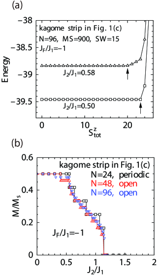
Figure 2: (Color)(a) Dependence of the lowest energy on $S_{\rm tot}^{z}$. The results of $J_{2}/J_{1}=0.5$ and $0.58$ for the system size of $N=96$ are presented. Arrows indicate the values of the spontaneous magnetization $M$ in each $J_{2}/J_{1}$. The position of an arrow is given by the highest $S_{\rm tot}^{z}$ value among those that give the common lowest energy. (b) $J_{2}/J_{1}$ dependence of $M/M_{\rm s}$ obtained from ED calculations for $N=24$ (black square) under the periodic boundary condition and DMRG calculation for $N=48$ (red triangle) and $96$ (blue inverted triangle) under the open boundary condition. Note that for $N=96$ in (a) and (b), we use $MS=900$ and $SW=15$ and, that for $N=48$ in (b), we use $MS=400$ and $SW=15$.

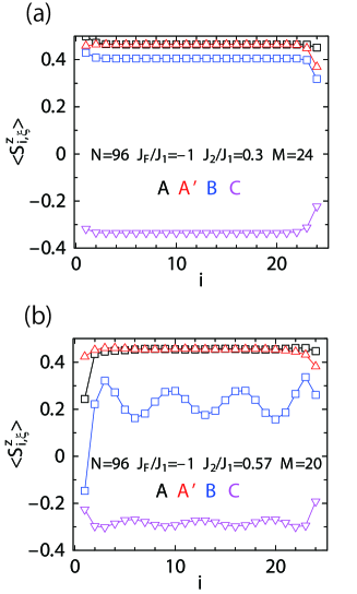
Figure 3: (Color) Local magnetization $\langle S_{i,\xi}^{z}\rangle$ at each sublattice $\xi$; A (black square), ${\rm A}^{\prime}$ (red triangle), B (blue square), and C (purple inverted triangle). Panels (a) and (b) show results for $J_{2}/J_{1}=0.3$ and $0.57$, respectively. These results are obtained from our DMRG calculations for $N=96$ ($i=1,2,\cdots,24$).

We examine the $J_{2}/J_{1}$ dependence of the ratio $M/M_{\rm s}$, where $M$ and $M_{\rm s}$ are the spontaneous and saturation magnetizations, respectively. Let us explain the method used to determine $M$ as a function of $N$ and $J_{2}/J_{1}$. First, we calculate the lowest energy $E(J_{2}/J_{1}$, $S_{\rm tot}^{z}$, $N)$, where $S_{\rm tot}^{z}$ value is the $z$-component of the total spin. For example, the energies for various $S_{\rm tot}^{z}$ in the two cases of $J_{2}/J_{1}$ are presented in Fig. 2(a); the results are obtained by our DMRG calculations of the system of $N=96$ with the maximum number of retained states ($MS$) of 600 and the number of sweeps ($SW$) of 15. The spontaneous magnetization $M(J_{2}/J_{1}$, $N$) is determined as the highest $S_{\rm tot}^{z}$ among those at the lowest common energy [see arrows in Fig. 2(a)]. Our results of the $J_{2}/J_{1}$ dependence of $M/M_{\rm s}$ are depicted in Fig. 2(b). We find the existence of the intermediate magnetic phase of $0<M/M_{\rm s}<1/2$ between the LM ferrimagnetic phase of $M/M_{\rm s}=1/2$ and the nonmagnetic phase. In order to determine the spin state of this intermediate phase, we calculate the local magnetization $\langle S_{i,\xi}^{z}\rangle$, where $\langle A\rangle$ denotes the expectation value of the physical quantity $A$ and $S_{i,\xi}^{z}$ is the $z$-component of ${\bf S}_{i,\xi}$. Figure 3 depicts our results for a system size $N=96$ on the lattice depicted in Fig. 1(c) under the open boundary condition; Figs. 3(a) and 3(b) correspond to the case of the LM ferrimagnetic phase and that of the intermediate phase, respectively.

The results clearly indicate the existence of the incommensurate modulation with long-distance periodicity in the intermediate phase. We also confirm that the periodicities of the local magnetizations in the NLM ferrimagnetism in the present model depend on the $J_{2}/J_{1}$ value but not on the length of the system, as reported in the case of ref. References.

It is worth emphasizing the point that the intermediate phase commonly exists irrespective of the shape at the edge of the strip lattice when one compares the result of the present lattice depicted in Fig. 1(c) and that in ref. References. Therefore, we can conclude that the intermediate phase exists and that it is NLM ferrimagnetic.

Although there exists an intermediate NLM ferrimagnetic phase in the case of the kagome strip lattice depicted in Fig. 1(c), we should note that there is a large discrepancy in dimensionality between the kagome strip lattice depicted in Fig. 1(c) and the 2D kagome lattice depicted in Fig. 1(a). In the next section, we treat the kagome strip lattice depicted in Fig. 1(b) whose width is larger than that of the kagome strip lattice depicted in Fig. 1(c).

IV Kagome Strip Lattice with Large Width

IV.1 Hamiltonian

In this section, we study the ground-state properties of the $S=1/2$ Heisenberg model on the kagome strip lattice depicted in Fig. 1(b). The Hamiltonian of this model is given by

$$\mathcal{H} = J_{1}\sum_{i}[{\bf S}_{i,{\rm B}}\cdot{\bf S}_{i,{\rm C}}+{\bf S}_{i,{\rm C}}\cdot{\bf S}_{i,{\rm D}}+{\bf S}_{i,{\rm C}}\cdot{\bf S}_{i+1,{\rm A}}+{\bf S}_{i,{\rm C}}\cdot{\bf S}_{i+1,{\rm B}}$$ (2)

$$+ {\bf S}_{i,{\rm C}^{\prime}}\cdot{\bf S}_{i,{\rm B}^{\prime}}+{\bf S}_{i,{\rm C}^{\prime}}\cdot{\bf S}_{i,{\rm A}^{\prime}}+{\bf S}_{i,{\rm C}^{\prime}}\cdot{\bf S}_{i+1,{\rm D}}+{\bf S}_{i,{\rm C}^{\prime}}\cdot{\bf S}_{i+1,{\rm B}^{\prime}}]$$

$$+ J_{2}\sum_{i}[{\bf S}_{i,{\rm A}}\cdot{\bf S}_{i,{\rm B}}+{\bf S}_{i,{\rm B}}\cdot{\bf S}_{i,{\rm D}}+{\bf S}_{i,{\rm D}}\cdot{\bf S}_{i,{\rm B}^{\prime}}+{\bf S}_{i,{\rm B}^{\prime}}\cdot{\bf S}_{i,{\rm A}^{\prime}}]$$

$$+ J_{\rm F}\sum_{i}[{\bf S}_{i,{\rm A}}\cdot{\bf S}_{i+1,{\rm A}}+{\bf S}_{i,{\rm A}^{\prime}}\cdot{\bf S}_{i+1,{\rm A}^{\prime}}]$$

$$- h\sum_{i}[S^{z}_{i,{\rm A}}+S^{z}_{i,{\rm A}^{\prime}}+S^{z}_{i,{\rm B}}+S^{z}_{i,{\rm B}^{\prime}}+S^{z}_{i,{\rm C}}+S^{z}_{i,{\rm C}^{\prime}}+S^{z}_{i,{\rm D}}].$$

Here, the positions of seven sublattices are denoted by A, ${\rm A}^{\prime}$, B, ${\rm B}^{\prime}$, C, ${\rm C}^{\prime}$, and D in Fig. 1(b). Note that the last term of eq. 2 is the Zeeman term. The number of spin sites is denoted by $N$. The number of unit cells is $N/7$; we consider $N/14$ as an integer. We mainly use the DMRG method for investigating the magnetic properties in the ground state of this Q1D system under the open boundary condition. We also investigate the properties under the periodic boundary condition by the ED method, although the size treated by this method is only in the case of $N=28$. Hereafter, we consider $J_{1}=1$ as an energy scale and we investigate the region of $0<J_{2}/J_{1}<\infty$ in the case of $J_{\rm F}=-1$.

IV.2 Phase diagram

First, let us examine the $J_{2}/J_{1}$ dependence of the ratio $M/M_{\rm s}$ in the absence of the external magnetic field $h$. The procedure for determining $M$ is the same as that mentioned in §3 [see also Fig. 4(a)]. We present our results of the spontaneous magnetization in Fig. 4(b). We successfully observe the intermediate-magnetization region irrespective of the boundary conditions. A careful observation of Fig. 4(b) enables us to observe the eight regions at least in the finite-size system. As a matter of convenience, hereafter, we call these regions ${\rm R}_{1}$, ${\rm R}_{2}$, $\cdots$, ${\rm R}_{7}$, and ${\rm R}_{8}$. In the case of $N=112$ under the open boundary condition, for example, Fig. 5(a) illustrates the regions ${\rm R}_{1}$ to ${\rm R}_{8}$: ${\rm R}_{1}$ is the region of $M/M_{\rm s}=3/7$, ${\rm R}_{2}$ is the region of $11/28\leq M/M_{\rm s}<3/7$, ${\rm R}_{3}$ is the region of $1/8<M/M_{\rm s}<11/28$, ${\rm R}_{4}$ is the region of $M/M_{\rm s}=1/8$, ${\rm R}_{5}$ is the region of $0<M/M_{\rm s}<1/8$, ${\rm R}_{6}$ is the region of $M/M_{\rm s}=0$, ${\rm R}_{7}$ is the region of $0<M/M_{\rm s}<1/7$, and ${\rm R}_{8}$ is the region of $M/M_{\rm s}=1/7$. Here, the dashed lines in Fig. 5(a) indicate the boundaries of these regions.

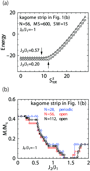
Figure 4: (Color)(a) Lowest energy in each subspace divided by $S_{\rm tot}^{z}$. The results of the DMRG calculations obtained when the system size is $N=56$ for $J_{2}/J_{1}=0.20$ and 0.57 are presented. Arrows indicate the spontaneous magnetization $M$ for a given $J_{2}/J_{1}$. (b) $J_{2}/J_{1}$ dependence of $M/M_{\rm s}$ obtained from the ED calculations for $N=$28 (blue triangle) under the periodic boundary condition and the DMRG calculations for $N=$56 (red square) and 112 (black pentagon) under the open boundary condition. Note that for $N=$ 56 in (a) and (b), we use $MS=$ 600 and $SW=$15, and that for $N=112$ in (b), we use $MS\geq$ 900 and $SW=$15. Here, $MS$ denotes the maximum number of retained states and $SW$ the number of sweeps used in DMRG calculations.

It should be noted that the values of $M/M_{\rm s}$ in the ${\rm R}_{4}$ region and that at the lower edge of the ${\rm R}_{2}$ region change with increasing $N$, as shown in Fig. 4(b); the former value is $M/M_{\rm s}=(N-14)/7N$ and the latter value is $M/M_{\rm s}=(3N-28)/7N$. These changes due to the increase in system size come from the finite-size effect. We find that the value of $M/M_{\rm s}$ in the ${\rm R}_{4}$ region under the open boundary condition increases and approaches the value of $M/M_{\rm s}=1/7$ when $N$ increases. Furthermore, the magnetization value in the ${\rm R}_{4}$ region is $M/M_{\rm s}=1/7$ in the case of $N=28$ under the periodic boundary condition. Therefore, it is expected that the value of $M/M_{\rm s}$ in the ${\rm R}_{4}$ region is $1/7$ in the thermodynamic limit. We also confirm that the value of $M/M_{\rm s}$ at the lower edge of the ${\rm R}_{2}$ region gradually increases and approaches the value of $M/M_{\rm s}=3/7$ with increasing $N$. In addition, we cannot confirm the ${\rm R}_{2}$ region in the case of $N=28$ under the periodic boundary condition. These circumstances indicate a possibility that the ${\rm R}_{2}$ region merges with the ${\rm R}_{1}$ region of $M/M_{\rm s}=3/7$ in the thermodynamic limit.

Next, to determine whether each region survives in the thermodynamic limit, we study the size dependences of the boundaries between the regions under the open boundary condition. Figure 5(b) shows the results of $N=$42, 56, 84, and 112 from DMRG calculations. Note here that we define ${\rm R}_{2}$ as the region of $(3N-28)/7N<M/M_{\rm s}<3/7$ and ${\rm R}_{4}$ as the region of $M/M_{\rm s}=(N-14)/7N$ in the finite-size system. One can find immediately from Fig. 5(b) that all regions, except the ${\rm R}_{7}$ region, survive in the limit $N\rightarrow\infty$. To determine whether the ${\rm R}_{7}$ region survives in the thermodynamic limit, we investigate the size dependence of the width of the ${\rm R}_{7}$ region in Fig. 6. This plot shows us that the width of the ${\rm R}_{7}$ region decreases with increasing $N$. It is difficult to determine whether the ${\rm R}_{7}$ region survives in the thermodynamic limit. The convex downward behavior is observed for large sizes so that the region might survive; however, the observed behavior may be one of the serious finite-size effects. The issue of establishing the presence or absence of the ${\rm R}_{7}$ region should be clarified in future studies.

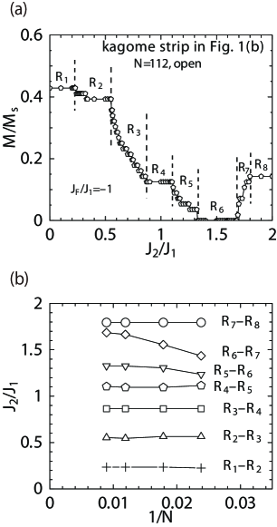
Figure 5: (a) Definitions of the ${\rm R}_{1}$-${\rm R}_{8}$ regions in the case of $N=112$ under the open boundary condition: ${\rm R}_{1}$ is the region of $M/M_{\rm s}=3/7$, ${\rm R}_{2}$ is the region of $11/28\leq M/M_{\rm s}<3/7$, ${\rm R}_{3}$ is the region of $1/8<M/M_{\rm s}<11/28$, ${\rm R}_{4}$ is the region of $M/M_{\rm s}=1/8$, ${\rm R}_{5}$ is the region of $0<M/M_{\rm s}<1/8$, ${\rm R}_{6}$ is the region of $M/M_{\rm s}=0$, ${\rm R}_{7}$ is the region of $0<M/M_{\rm s}<1/7$, and ${\rm R}_{8}$ is the region of $M/M_{\rm s}=1/7$. Dashed lines indicate the boundaries of these regions. (b) Size dependences of boundaries under the open boundary condition. The results presented are those of $N=$42, 56, 84, and 112 from DMRG calculations. The curve line named ${\rm R}_{l}$-${\rm R}_{l+1}$ indicates the boundary line between the ${\rm R}_{l}$ and ${\rm R}_{l+1}$ regions, where $l$ is integer.

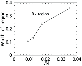
Figure 6: Size dependence of the width of the ${\rm R}_{7}$ region. It is difficult to determine whether the ${\rm R}_{7}$ region survives in the thermodynamic limit.

IV.3 Magnetic properties in each region

In this subsection, we investigate the local magnetization $\langle S_{i,\xi}^{z}\rangle$ to study the magnetic structures in various regions except the ${\rm R}_{2}$ and ${\rm R}_{6}$ regions. Note that we calculate $\langle S_{i,\xi}^{z}\rangle$ within the subspace of the highest $S_{\rm tot}^{z}$ corresponding to the spontaneous magnetization $M$ when $J_{2}/J_{1}$ is given. Considering the fact that the present lattice depicted in Fig. 1(b) has seven sublattices in the system, we will use different colors or symbols for each sublattice $\xi$ for presenting our results of $\langle S_{i,\xi}^{z}\rangle$, as depicted in the inset of Fig. 7(a); we use a black square for $\xi=$A, a red triangle for $\xi={\rm A}^{\prime}$, a blue cross for $\xi={\rm B}$, a green pentagon for $\xi={\rm B}^{\prime}$, a purple inverted triangle for $\xi=$C, an aqua diamond for $\xi={\rm C}^{\prime}$, and a black circle for $\xi=$D.

First, we examine the ${\rm R}_{1}$ and ${\rm R}_{8}$ regions. We present our DMRG results of $\langle S_{i,\xi}^{z}\rangle$ of the system of $N=112$ in Figs. 7(a) and 7(b) for $J_{2}/J_{1}=0.2$ and 1.9, respectively. In Fig. 7(a), we observe the uniform behavior of upward-direction spins at the sublattice sites A, ${\rm A}^{\prime}$, B, ${\rm B}^{\prime}$, and D, and downward-direction spins at the sublattice sites C and ${\rm C}^{\prime}$. In Fig. 7(b), we also observe the uniform behavior of upward-direction spins at the sublattice sites B, ${\rm B}^{\prime}$, C, and ${\rm C}^{\prime}$, and downward-direction spins at the sublattice sites A, ${\rm A}^{\prime}$, and D. Therefore, we conclude that the LM ferrimagnetic states are realized in the regions of ${\rm R}_{1}$ and ${\rm R}_{8}$.

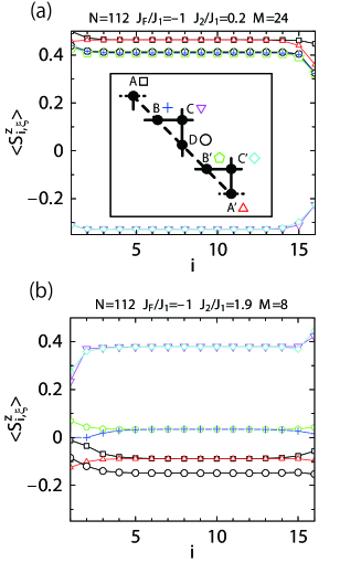
Figure 7: (Color) Local magnetization $\langle S_{i,\xi}^{z}\rangle$ at each sublattice $\xi$. Panels (a) and (b) show results for $J_{2}/J_{1}=$0.2 and 1.9, respectively. These results are obtained from our DMRG calculations for $N=112$ ($i=$1, 2, $\cdots$, 16). The inset in the panel (a) presents the correspondence relationship between each colored symbol and each sublattice $\xi$ used in Figs. 7, 9, and 10.

Our understanding of the origins of these LM ferrimagnetic phases is based on the Marshall-Lieb-Mattis (MLM) theorem. In the case of $J_{2}/J_{1}=0$, no frustration occurs; thus, the spin state depicted in Fig. 8(a) is realized. This state shows the LM ferrimagnetism with $M/M_{\rm s}=3/7$. The ${\rm R}_{1}$ region is directly connected to the LM ferrimagnetic state of $J_{2}/J_{1}=0$. Therefore, the ${\rm R}_{1}$ region of $M/M_{\rm s}=3/7$ is regarded as the LM ferrimagnetic phase. In the limit $J_{2}\rightarrow\infty$, on the other hand, the present model becomes equal to a model of an $S=1/2$ diamond chain depicted in Fig. 8(b). The value of magnetization takes $M/M_{\rm s}=1/7$ in the ground state of this diamond chain according to the MLM theorem. Therefore, the ${\rm R}_{8}$ region of $M/M_{\rm s}=1/7$ is regarded as the LM ferrimagnetic phase.

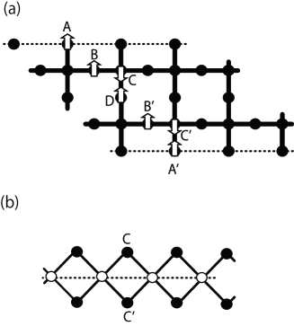
Figure 8: (a) Kagome strip lattice depicted in Fig. 1(b) in the limit of $J_{2}/J_{1}=0$. White arrowheads denote the classical spin configuration in the LM ferrimagnetic state of $M/M_{\rm s}=3/7$. (b) Kagome strip lattice depicted in Fig. 1(b) in the limit of $J_{2}\rightarrow\infty$. White circles represent the effective $S=1/2$ spins formed by five $S=1/2$ spins at the sublattices $\xi=$A, ${\rm A}^{\prime}$, B, ${\rm B}^{\prime}$, and D. The black bold and black dotted lines show the antiferromagnetic and ferromagnetic interactions, respectively.

Next, we investigate the ${\rm R}_{3}$, ${\rm R}_{5}$, and ${\rm R}_{7}$ regions. Our results obtained from the DMRG calculations of $N=168$ are depicted in Figs. 9(a)-9(c) for $J_{2}/J_{1}=0.57$, 1.14, and 1.69, respectively. We clearly observe incommensurate modulations with long-distance periodicities in every case in Fig. 9. In addition, we confirm from Fig. 4(b) that the ratio $M/M_{\rm s}$ changes gradually with the variation in $J_{2}/J_{1}$ in the R₃, R₅, and R₇ regions. Since the widths of the R₃ and R₅ regions survive in the thermodynamic limit as was clarified in the previous subsection, we conclude that the ${\rm R}_{3}$ and ${\rm R}_{5}$ regions are NLM ferrimagnetic phases. Although it is unclear whether the ${\rm R}_{7}$ region survives in the thermodynamic limit, this region is an NLM ferrimagnetic phase if it survives.

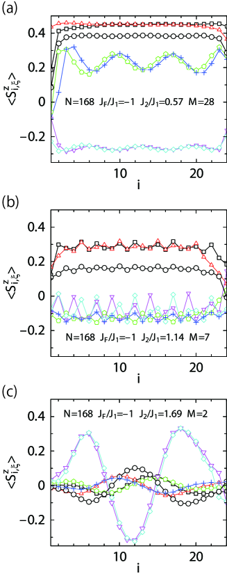
Figure 9: (Color) Local magnetization $\langle S_{i,\xi}^{z}\rangle$ at each sublattice $\xi$. The correspondence relationship between each colored symbol and each sublattice $\xi$ is described in the inset in Fig. 7(a). Panels (a), (b), and (c) show results for $J_{2}/J_{1}=$0.57, 1.14, and 1.69, respectively. These results are obtained from our DMRG calculations for $N=168$ ($i=$1, 2, $\cdots$, 24).

Finally, in this subsection, we examine the ${\rm R}_{4}$ region. Our result of $\langle S_{i,\xi}^{z}\rangle$ for $J_{2}/J_{1}=1$ in the system of $N=168$ is depicted in Fig. 10. We do not detect the incommensurate modulation in this ${\rm R}_{4}$ region. In addition, we confirm from Fig. 4(b) that the ratio $M/M_{\rm s}$ in the ${\rm R}_{4}$ region does not change with the variation in $J_{2}/J_{1}$ in contrast to the cases in the R₃ and R₅ regions. These circumstances suggest that the ${\rm R}_{4}$ region is the LM ferrimagnetic phase.

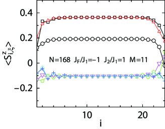
Figure 10: (Color) Local magnetization $\langle S_{i,\xi}^{z}\rangle$ at each sublattice $\xi$. This result is obtained from our DMRG calculations for $J_{2}/J_{1}=1$ in the system of $N=168$ ($i=$1, 2, $\cdots$, 24). The correspondence relationship between each colored symbol and each sublattice $\xi$ is described in the inset in Fig. 7(a).

However, one cannot speculate the spin state from the result of $\langle S_{i,\xi}^{z}\rangle$ because it is difficult to clarify the spin state on the basis of the results of determining whether the spins are up or down, as was successfully observed in the ${\rm R}_{8}$ region. We further investigate the magnetization curve in this region to know whether the ${\rm R}_{4}$ region is the LM ferrimagnetic phase. The magnetization curves of $J_{2}/J_{1}=1$ for $N=56$ and $N=112$ calculated by the DMRG method are presented in Fig. 11(a)comment . Figure 11(b) is obtained by zooming the region of $h$ near $h=0$. One can observe the existence of the magnetization plateaus at the height of the spontaneous magnetization for both system sizes. We also confirm that the difference in the width of the plateau between $N=112$ and 56 is very small. These features indicate that the spin gap exists in the ${\rm R}_{4}$ region in the thermodynamic limit. If the ${\rm R}_{4}$ region is the NLM ferrimagnetic phase, no spin gap is present in this region. (It was reported in ref. References that the NLM ferrimagnetism is gapless as a response to a uniform magnetic field.) Therefore, we conclude that the ${\rm R}_{4}$ region is the LM ferrimagnetic phase.

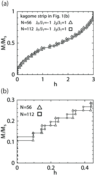
Figure 11: Magnetization curve in the ${\rm R}_{4}$ region. Panel (a) is obtained from the DMRG calculations of $J_{2}/J_{1}=1$ for $N=56$ (triangle) and $N=112$ (square). Panel (b) is obtained by zooming the region near $h=0$ in panel (a).

V Discussion

We discuss the relationships between the interval $0<J_{2}/J_{1}\leq 1$ of the kagome strip lattice depicted in Fig. 1(b) and those of the spatially anisotropic kagome lattice studied in ref. References, while we consider the case of another new lattice, with a larger but finite width along the direction perpendicular to the bonds of interaction $J_{\rm F}$ in Fig. 1(b), namely, the strip width.

The ratio $M/M_{\rm s}$ of the ${\rm R}_{1}$ and ${\rm R}_{2}$ regions is commonly $M/M_{\rm s}=3/7$ in the thermodynamic limit of the lattice depicted in Fig. 1(b). The difference of $M/M_{\rm s}=3/7$ from $M/M_{\rm s}=1/3$ in the case of the LM ferrimagnetic phase of the spatially anisotropic kagome lattice in ref. References is attributed to the finiteness of the strip width. Thus, the ratio $M/M_{\rm s}$ approaches $M/M_{\rm s}=1/3$ when the strip width increases; the ${\rm R}_{1}$ and ${\rm R}_{2}$ regions of the present model depicted in Fig. 1(b) correspond to the LM ferrimagnetic phase of the spatially anisotropic kagome lattice studied in ref. References.

The ratio $M/M_{\rm s}=1/7$ at $J_{2}/J_{1}=1$ in the present model depicted in Fig. 1(b) may be related to the fact that the model includes seven sublattices, namely, the strip width is finite. At least at $J_{2}/J_{1}=1$, on the other hand, it is widely believed that the spontaneous magnetization disappears in the limit of infinite widthLecheminant ; Waldtmann ; Hida_kagome ; Cabra ; Honecker0 ; Honecker1 ; Cepas ; Spin_gap_Sindzingre ; HN_Sakai2010 ; Sakai_HN_PRBR ; HN_Sakai2011 . Although the relationship should be clarified in the examination of the case of the lattice with an even larger strip width, there are two possibilities of the behavior near the case of $J_{2}/J_{1}=1$. One is the case when the ratio $M/M_{\rm s}$ decreases with increasing strip width and finally vanishes, while the LM ferrimagnetic phase, such as ${\rm R}_{4}$, survives in systems with larger strip widths. In this case, the ${\rm R}_{3}$ region corresponds to the NLM phase of the two-dimensional model on the spatially anisotropic kagome lattice. In the other case, the LM ferrimagnetic phase, such as ${\rm R}_{4}$, becomes narrower with increasing strip width, while the ratio $M/M_{\rm s}$ does not vanish; finally, the ${\rm R}_{3}$ and ${\rm R}_{5}$ regions merge with each other. In this case, the value of $J_{2}/J_{1}$ at the boundary between the ${\rm R}_{5}$ and ${\rm R}_{6}$ regions decreases across $J_{2}/J_{1}=1$. In any cases, it is important to note that from our finding of an intermediate phase in all the three cases in Fig. 1 between the ferrimagnetic phase and the nonmagnetic phase, the phase is considered to exist irrespective of the strip width.

Finally, one should note that the intermediate phase between the Lieb-Mattis ferrimagnetic and nonmagnetic states is observed in other cases. However, this phase is not always ferrimagnetic. One of the cases observed is the case of the three-leg ladder system forming a strip lattice obtained by cutting off from the spatially anisotropic triangular lattice in ref. References, in which the properties of the intermediate phase were unclear. Sakai’s unpublished study suggests that the intermediate phase is nematicSakai_private_com . Careful examinations are required to investigate such an intermediate phase if it is found.

VI Summary

We have studied the ground-state properties of the $S=1/2$ Heisenberg models on the kagome strip lattices depicted in Figs. 1(b) and 1(c) by the ED and DMRG methods. As a common phenomenon in the ground state of both cases, we have confirmed the existence of the non-Lieb-Mattis ferrimagnetism between the Lieb-Mattis ferrimagnetic phase and the nonmagnetic phase. We have clearly found incommensurate modulations with long-distance periodicity in the non-Lieb-Mattis ferrimagnetic state. The occurrence of the non-Lieb-Mattis ferrimagnetism irrespective of strip width strongly suggests that the intermediate state found in the case of the spatially anisotropic kagome lattice in two dimensions is the non-Lieb-Mattis ferrimagnetism.

References

- (1) E. Lieb and D. Mattis: J. Math. Phys. 3 (1962) 749.
- (2) W. Marshall: Proc. Roy. Soc. A 232 (1955) 48.
- (3) K. Takano, K. Kubo, and H. Sakamoto: J. Phys.: Condens. Matter 8 (1996) 6405.
- (4) K. Okamoto, T. Tonegawa, Y. Takahashi, and M. Kaburagi: J. Phys.: Condens. Matter 11 (1999) 10485.
- (5) T. Tonegawa, K. Okamoto, T. Hikihara, Y. Takahashi, and M. Kaburagi: J. Phys. Soc. Jpn. 69 (2000) Suppl. A, 332.
- (6) T. Sakai and K. Okamoto: Phys. Rev. B 65 (2002) 214403.
- (7) N. B. Ivanov and J. Richter: Phys. Rev. B 69 (2004) 214420.
- (8) S. Yoshikawa and S. Miyashita: Stastical Physics of Quantum Systems:novel orders and dynamics, J. Phys. Soc. Jpn. 74 (2005) Suppl., p. 71.
- (9) K. Hida: J. Phys.: Condens. Matter 19 (2007) 145225.
- (10) K. Hida and K. Takano: Phys. Rev. B 78 (2008) 064407.
- (11) R. R. Montenegro-Filho and M. D. Coutinho-Filho: Phys. Rev. B 78 (2008) 014418.
- (12) T. Shimokawa and H. Nakano: J. Phys. Soc. Jpn. 80 (2011) 043703.
- (13) T. Shimokawa and H. Nakano: J. Phys. Soc. Jpn. 80 (2011) 125003.
- (14) N. B. Ivanov, J. Richter, and D. J. J. Farnell: Phys. Rev. B 66 (2002) 014421.
- (15) R. F. Bishop, P. H. Y. Li, D. J. J. Farnell, and C. E. Campbell: Phys. Rev. B 82 (2010) 024416.
- (16) H. Nakano, T. Shimokawa, and T. Sakai: J. Phys. Soc. Jpn. 80 (2011) 033709.
- (17) P. Lecheminant, B. Bernu, C. Lhuillier, L. Pierre, and P. Sindzingre: Phys. Rev. B 56 (1997) 2521.
- (18) Ch. Waldtmann, H.-U. Everts, B. Bernu, C. Lhuillier, P. Sindzingre, P. Lecheminant, and L. Pierre: Eur. Phys. J. B 2 (1998) 501.
- (19) K. Hida: J. Phys. Soc. Jpn. 70 (2001) 3673.
- (20) D. C. Cabra, M. D. Grynberg, P. C. W. Holdsworth, and P. Pujol: Phys. Rev. B 65 (2002) 094418.
- (21) J. Schulenberg, A. Honecker, J. Schnack, J. Richter, and H.-J. Schmidt: Phys. Rev. Lett. 88 (2002) 0167207.
- (22) A. Honecker, J. Schulenberg, and J. Richter: J. Phys.: Condens. Matter 16 (2004) S749.
- (23) O. Cepas, C. M. Fong, P. W. Leung, and C. Lhuillier: Phys. Rev. B 78 (2008) 140405(R).
- (24) P. Sindzingre and C. Lhuillier: Europhys. Lett. 88 (2009) 27009.
- (25) H. Nakano and T. Sakai: J. Phys. Soc. Jpn. 79 (2010) 053707.
- (26) T. Sakai and H. Nakano: Phys. Rev. B 83 (2011) 100405(R).
- (27) H. Nakano and T. Sakai: J. Phys. Soc. Jpn. 80 (2011) 053704.
- (28) P. Azaria, C. Hooley, P. Lecheminant, C. Lhuillier, and A. M. Tsvelik: Phys. Rev. Lett. 81 (1998) 1694.
- (29) Ch. Waldtmann, H. Kreutzmann, U. Schollwock, K. Maisinger, and H.-U. Everts: Phys. Rev. B 62 (2000) 9472.
- (30) J. Schulenburg, A. Honecker, J. Schnack, J. Richter, and H.-J. Schmidt: Phys. Rev. Lett. 88 (2002) 167207.
- (31) T. Shimokawa and H. Nakano: J. Phys.: Conf. Ser. 320 (2011) 012007.
- (32) S. R. White: Phys. Rev. Lett. 69 (1992) 2863.
- (33) S. R. White: Phys. Rev. B 48 (1993) 10345.
- (34) One can find the macroscopic jump in this magnetization curve near the saturation field as well as in the case of some frustrated systemskagome-strip3 ; localized-magnon . It is known that the occurrence mechanism of the magnetization jump can be understood from the viewpoint of the localized-magnon picture (see refs. References, References, and References).
- (35) J. Schnack, H.-J. Schmidt, A. Honecker, J. Schulenburg, and J. Richter: J. Phys.: Conf. Ser. 51 (2006) 43.
- (36) M. E. Zhitomirsky and H. Tsunetsugu: Phys. Rev. B 70 (2004) 100403.
- (37) S. Abe, T. Sakai, K. Okamoto, and K. Tutsui: J. Phys.: Conf. Ser. 320 (2011) 012015.
- (38) T. Sakai: private communications.
- (39) A. F. Albuquerque, F. Alet, P. Corboz, P. Dayal, A. Feiguin, L. Gamper, E. Gull, S. Gurtler, A. Honecker, R. Igarashi, M. Korner, A. Kozhevnikov, A. Lauchli, S. R. Manmana, M. Matsumoto, I. P. McCulloch, F. Michel, R. M. Noack, G. Pawlowski, L. Pollet, T. Pruschke, U. Schollwock, S. Todo, S. Trebst, M. Troyer, P. Werner, and S. Wessel: J. Magn. Magn. Mater. 310 (2007) 1187 (see also http://alps.comp-phys.org).