Group Iterative Spectrum Thresholding for Super-Resolution Sparse Spectral Selection

Abstract

Recently, sparsity-based algorithms are proposed for super-resolution spectrum estimation. However, to achieve adequately high resolution in real-world signal analysis, the dictionary atoms have to be close to each other in frequency, thereby resulting in a coherent design. The popular convex compressed sensing methods break down in presence of high coherence and large noise. We propose a new regularization approach to handle model collinearity and obtain parsimonious frequency selection simultaneously. It takes advantage of the pairing structure of sine and cosine atoms in the frequency dictionary. A probabilistic spectrum screening is also developed for fast computation in high dimensions. A data-resampling version of high-dimensional Bayesian Information Criterion is used to determine the regularization parameters. Experiments show the efficacy and efficiency of the proposed algorithms in challenging situations with small sample size, high frequency resolution, and low signal-to-noise ratio.

Keywords: spectral estimation, sparsity, super-resolution, nonconvex optimization, iterative thresholding, model selection, spectra screening.

I Introduction

The problem of spectral estimation studies how signal power is distributed over frequencies, and has rich applications in speech coding, radar & sonar signal processing and many other areas. Suppose a discrete-time real-valued signal is observed at finite time points contaminated with i.i.d. Gaussian noise. In common with all spectral models, we assume the signal can be represented as a linear combination of sinusoids, and aim to recover the spectrum of the signal at a desired resolution. However, the problem becomes very challenging when the required frequency resolution is high. In particular, the number of the frequency levels at the desired resolution can be (much) greater than the sample size, referred to as super-resolution spectral estimation. For such discrete-time signals of finite length, the classical methods based on fourier analysis [1] or least-squares periodogram (LSP) [2, 3] suffer from power leakage and have very limited spectral resolution [1]. Some more recent algorithms, such as Burg [1], MUSIC [4] and RELAX [5] only alleviate the issue to some extent.

We assume that the signal is sparse in the frequency-domain, i.e., the number of its sinusoidal components is small relative to the sample size, referred to as the spectral sparsity. It is a realistic assumption in many applications (e.g., astronomy [6] and radar signal processing [7]), and makes it possible to apply the revolutionary compressed sensing (CS) technique. In [6], Chen and Donoho proposed the basis pursuit (BP) to handle overcomplete dictionaries and unevenly sampled signals. A number of similar works followed, see, e.g., [8, 9, 10, 11, 12, 13, 14, 15] and the references therein.

We point out two crucial facts that cannot be ignored in super-resolution spectrum reconstruction. (a) When the desired frequency resolution is very high, neighboring dictionary atoms become very similar and thus necessarily result in high coherence or collinearity. As is well known in the literature, the popular convex $l_{1}$ technique as used in the BP yields inconsistent frequency selection and suboptimal rates in estimation and prediction under such coherent setups [16, 17, 18, 19, 20]. (b) The grouping structure of the sinusoidal components is an essential feature in spectrum recovery: if frequency $f$ is absent in the signal, the coefficients for $\cos(2\pi ft)$ and $\sin(2\pi ft)$ should both be zero.

In this paper we investigate super-resolution spectral recovery from a statistical perspective and propose a group iterative spectrum thresholding (GIST) framework to tackle the aforementioned challenges. GIST allows for (possibly nonconvex) shrinkage estimation and can exploit the pairing structure. Interestingly, we find that neither the $l_{1}$ nor the $l_{0}$ regularization is satisfactory for spectrum estimation, and advocate a hybrid $l_{0}+l_{2}$ type shrinkage estimation. Theoretical analysis shows that the new regularization essentially removes the stringent coherence requirement and can accommodate much lower SNR and higher coherence. Furthermore, a GIST variant provides a screening technique for supervised dimension reduction to deal with applications in ultrahigh dimensions. The rest of this paper is organized as follows. We formulate the problem from a statistical point of view and briefly survey the literature in Section II. In Section III, we propose the GIST framework—in more details, a novel form of regularization, a generic algorithm for fitting group nonconvex penalized models, a data-resampling based model selection criterion, and a probabilistic spectral screening for fast computation. Experimental results are shown in Section IV. We summarize the conclusions in Section V. The technical details are left to the Appendices.

II Model Setup and The Super-resolution Challenge

In this section, we introduce the problem of super-resolution spectrum estimation and review some existing methods from a statistical point of view. Let ${\boldsymbol{y}}=[y(t_{n})]_{1\leq n\leq N}$ be a real-valued signal contaminated with i.i.d. Gaussian noise $N(0,\sigma^{2})$. (We focus on real signals in this paper but our methodology carries over to complex-valued signals; see Section V.) The sampling time sequence $\{t_{n}\}_{1\leq n\leq N}$ is not required to be uniform (cf. [6]). In order to achieve super-resolution spectral recovery, an overcomplete frequency dictionary must be applied. Concretely, we use a grid of evenly spaced frequencies $f_{k}=f_{\max}\cdot k/D$ for $k=0,1,\cdots,D$ to construct the sine and cosine frequency predictors, i.e., $\cos(2\pi tf_{k})$ and $\sin(2\pi tf_{k})$. Let $\mathcal{F}$ denote the set of nonzero frequencies $\{f_{1},\cdots,f_{D}\}$. The upper band limit $f_{\max}$ can be $(2\min_{1\leq n\leq N}(t_{n}-t_{n-1}))^{-1}$ or estimated based on the spectral window [21]. The cardinality of the dictionary controls the frequency resolution given by $f_{\max}/D$. The true spectra of the signal are assumed to be discrete for convenience, because the quantization error can always be reduced by increasing the value of $D$. The signal can be represented by

$$y_{n}=y(t_{n})=\sum_{k=0}^{D}A_{k}\cos(2\pi f_{k}t_{n}+\phi_{k})+e_{n},1\leq n\leq N,$$ (1)

where $A_{k}$, $\phi_{k}$ are unknown, and the noise $\{e_{n}\}_{n=1}^{N}$ are i.i.d. Gaussian with zero mean and unknown variance $\sigma^{2}$. Traditionally, $D\leq N$. But in super resolution spectral analysis, $D$ can take a much larger value than $N$. It still results in a well-defined problem because only a few $A_{k}$ are nonzero under the spectral sparsity assumption.

From $A_{k}\cos(2\pi f_{k}t_{n}+\phi_{k})$ $=A_{k}\cos(\phi_{k})\cos(2\pi f_{k}t_{n})-A_{k}\sin(\phi_{k})\sin(2\pi f_{k}t_{n})$ $=a_{k}\cos(2\pi f_{k}t_{n})+b_{k}\sin(2\pi f_{k}t_{n})$ with $a_{k}=A_{k}\cos\phi_{k}$, $b_{k}=-A_{k}\sin\phi_{k}$, we introduce two column vectors

$${\boldsymbol{X}}^{\cos}(f)\triangleq\left[\cos(2\pi t_{n}f)\right]_{1\leq n\leq N},$$

$${\boldsymbol{X}}^{\sin}(f)\triangleq\left[\sin(2\pi t_{n}f)\right]_{1\leq n\leq N},$$

and define the predictor matrix

$${\boldsymbol{X}}\triangleq[{\boldsymbol{X}}^{\cos}(f_{1}),\cdots,{\boldsymbol{X}}^{\cos}(f_{D}),{\boldsymbol{X}}^{\sin}(f_{1}),\cdots,{\boldsymbol{X}}^{\sin}(f_{D})].$$ (2)

(Some redundant or useless predictors can be removed in concrete problems, see (4).) Denote the coefficient vector by ${\boldsymbol{\beta}}\in{\mathbb{R}}^{2D}$ and the intercept (zero frequency component) by $\alpha$. Now the model can be formulated as a linear regression

$${\boldsymbol{y}}=\alpha+{\boldsymbol{X}}{\boldsymbol{\beta}}+\boldsymbol{e},$$ (3)

where ${\boldsymbol{\beta}}$ is sparse and $\boldsymbol{e}\sim N(\mathbf{0},\sigma^{2}{\boldsymbol{I}})$. In super-resolution analysis, $D\gg N$, giving a small-sample-size-high-dimensional design. Linear analysis such as Fourier transform fails for such an underdetermined system.

As a demonstration, we consider a noisy ‘TwinSine’ signal at frequencies $0.25$ Hz and $0.252$ Hz with 100 observations. Obviously, the frequency resolution needs to be as fine as $0.002$ HZ to perceive and distinguish the two sinusoidal components with different coefficients. We set $f_{\max}=1/2$, and thus $2D$ must be at least $500$ – much larger than the sample size. The concrete design matrix (without the intercept) is given by

$${\boldsymbol{X}}=\left[\begin{smallmatrix}\cos(\pi\frac{1}{D}t_{1})&\cdots&\cos(\pi\frac{D}{D}t_{1})&\sin(\pi\frac{1}{D}t_{1})&\cdots&\sin(\pi\frac{D-1}{D}t_{1})\\ \vdots&\vdots&\vdots\quad&\vdots&\vdots&\vdots\\ \cos(\pi\frac{1}{D}t_{N})&\cdots&\cos(\pi\frac{D}{D}t_{N})&\sin(\pi\frac{1}{D}t_{N})&\cdots&\sin(\pi\frac{D-1}{D}t_{N})\\ \end{smallmatrix}\right].$$ (4)

The last sine atom disappears because all $t_{n}$ are integers. This yields a super-resolution spectral estimation problem.

There are many algorithms for identifying the spectrum of a discrete-time signal. But not all of them can super-resolve. From a modeling perspective, we classify them as nonsparse methods and sparse methods. Most classical methods (e.g., [3, 21, 2]) are nonsparse and assume no knowledge on the power spectra. For super-resolution spectrum estimation, they may seriously broaden the main lobes and introduce side lobes. In this paper, we focus on sparse methods. As aforementioned, one popular assumption for solving underdetermined systems is signal sparsity: the number of present frequency components is small relative to the number of samples. The problem is still NP hard because the frequency location of the truly relevant sinusoidal components is unknown and the number of candidate components can be very large. In fact, the frequency grid used for constructing the dictionary can be made arbitrarily fine by the customer.

Early attempts to enforce sparsity effects include greedy or exhaustive searches [22, 23] and genetic algorithms with a sparsity constraint [24]. Harikumar [25] computes the maximally sparse solutions under a constraint on the fitting error. A breakthrough is due to Chen & Donoho who proposed the basis pursuit (BP) for spectrum estimation [6]. A number of similar works followed [11, 8, 9, 10]. BP is able to superresolve for unevenly sampled signals. In our notation, the noiseless version of BP solves the convex optimization problem $\min||{\boldsymbol{\beta}}||_{1}\text{ s.t. }\alpha+{\boldsymbol{X}}{\boldsymbol{\beta}}={\boldsymbol{y}}.$ The noisy versions can be defined similarly, in a penalty/constraint form. The $l_{1}$-norm provides the tightest convex relaxation to the $l_{0}$-norm and achieves a sparse spectral representation of the signal within feasible time and cost.

In recent years, the power and limitation of this convex relaxation have been systematically studied in a large body of compressed sensing literature. In short, to guarantee good statistical performance in either prediction, estimation, or model selection, the coherence of the system must be low, in terms of, e.g., mutual coherence conditions [16], restricted isometry property (RIP) [17] and irrepresentable conditions [19] among others. For example, the RIP of order $s$ requires that for any index set $I\subset\mathcal{F}$ with $|I|=s$, there exists an RIP constant $\delta_{s}\geq 0$ such that $(1-\delta_{s})\|{\boldsymbol{v}}\|_{2}^{2}\leq\|{\boldsymbol{X}}_{I}{\boldsymbol{v}}\|_{2}^{2}\leq(1+\delta_{s})\|{\boldsymbol{v}}\|_{2}^{2}$, $\forall v\in\mathbb{R}^{s}$; when $\delta_{s}$ is small, any $s$ predictors in ${\boldsymbol{X}}$ are approximately orthogonal. In theory, to guarantee $l_{1}$’s effectiveness in statistical accuracy, frequency selection consistency, and algorithmic stability, such RIP constants have to be small, e.g., $\delta_{3S}+3\delta_{4S}<2$ in a noisy setup, where $S=\|{\boldsymbol{\beta}}\|_{0}$ [17]. Similarly, the mutual coherence, defined as the maximum absolute value of the off-diagonal elements in the scaled Gram matrix ${\boldsymbol{X}}^{T}{\boldsymbol{X}}/N$, has to be as low as $O(1/S)$ [16]. Such theoretical results clearly indicate that the super-resolution challenge cannot be fully addressed by the $l_{1}$-norm based methods, because many similar sinusoidal components may arise in the dictionary and bring in high coherence.

To enhance the sparsity of the BP, Blumensath & Davies proposed the iterative hard thresholding (IHT) [12, 13]. See [14, 15] for some approximation methods. Intuitively, nonconvex penalties can better approximate the $l_{0}$-norm and yield sparser estimates than the convex $l_{1}$-penalty. On the other hand, we find that when the signal-to-noise ratio (SNR) is low and/or the coherence is high, the $l_{0}$ penalization may give an over-sparse spectral estimate and miss certain true frequency components. The high miss rates are due to the fact that the $l_{0}$ regularization is through (hard) thresholding only, offering no shrinkage at all for nonzero coefficients. Therefore, it tends to kill too many predictors to achieve the appropriate extent of shrinkage especially when the SNR is low. An inappropriate nonconvex penalty may seriously mask true signal components. This issue will be examined in the next section.

III GIST Framework

This section examines the super-resolution spectrum estimation in details. The complete group iterative spectrum thresholding (GIST) framework is introduced at the end.

III-A A novel regularization form

In this subsection, we study a group penalized least-squares model and investigate the appropriate type of regularization.

The BP finds a solution to an underdetermined linear system with the minimum $l_{1}$ norm. When the signal is corrupted by noise as in (3), the following $l_{1}$-penalized linear model is more commonly used:

$${1\over 2}\|{\boldsymbol{y}}-\alpha-{\boldsymbol{X}}{\boldsymbol{\beta}}\|_{2}^{2}+\lambda\|{\boldsymbol{\beta}}\|_{1},$$ (5)

where $\lambda$ is a regularization parameter to provide a trade-off between the fitting error and solution sparsity. The intercept or zero frequency component $\alpha$ is not subject to any penalty. To include more sparsity-enforcing penalties, we consider a more general problem in this paper which minimizes

$${1\over 2}\|{\boldsymbol{y}}-\alpha-{\boldsymbol{X}}{\boldsymbol{\beta}}\|_{2}^{2}+\sum_{k=1}^{2D}P(|\beta_{k}|;\lambda)=:F({\boldsymbol{\beta}};\lambda),$$ (6)

where $P(\cdot;\lambda)$ is a univariate penalty function parameterized by $\lambda$ and is possibly nonconvex.

Some structural information can be further incorporated in spectrum estimation. From the derivation of (3), $A_{k}=0$ implies $\beta_{k}=\beta_{D+k}=0$, i.e., the sine and cosine predictors at $f_{k}$ vanish simultaneously. The pairing structure shows it is more reasonable to impose the so-called group sparsity or block sparsity [26, 27] on $\{(\beta_{k},\beta_{D+k})\}_{1\leq k\leq D}$ rather than the unstructured sparsity on $\{\beta_{k}\}_{1\leq k\leq 2D}$. The group penalized model with the model design (2) minimizes

$${1\over 2}\|{\boldsymbol{y}}-\alpha-{\boldsymbol{X}}{\boldsymbol{\beta}}\|_{2}^{2}+\sum_{k=1}^{D}P\left(\sqrt{\beta_{k}^{2}+\beta_{D+k}^{2}};\lambda\right)=:F({\boldsymbol{\beta}};\lambda).$$ (7)

(In the problem with the design matrix given by (4), the last sine predictor disappears and thus we always set $\beta_{2D}$ to be $0$.) The penalty function $P$ is the same as before and is allowed to be nonconvex. For ease in computation, the first term in (6) and (7) will be replaced by ${1\over 2}\|{\boldsymbol{y}}-\alpha-{\boldsymbol{X}}{\boldsymbol{\beta}}\|_{2}^{2}/C$ for some $C$ large enough; see the comment after Theorem 1.

A crucial problem is then to determine the appropriate form of $P$ for regularization purposes. The popular $l_{1}$-penalty $P_{1}(t;\lambda)=\lambda|t|$ may result in insufficient sparsity and relatively large prediction error, as shown in Section IV. There is still much room for improvement in super-resolution spectral estimation. Before we proceed, it is worth pointing out that there are two objectives involved in this task
Objective 1 (O1): accurate prediction of the signal at any new time point in the time domain;
Objective 2 (O2): parsimonious spectral representation of the signal in the Fourier domain.
O1+O2 complies with Occam’s razor principle—the simplest way to explain the data is the best. A perfect approach must reflect both concerns to produce a stable sparse model with good generalizability.

From the perspective of O2, the $l_{0}$-norm constructs an ideal penalty

$$P_{0}(t;\lambda)=\frac{\lambda^{2}}{2}1_{t\neq 0},$$ (8)

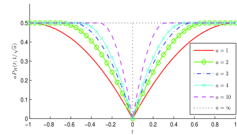
where the indicator function $1_{t\neq 0}$ is $1$ when $t\neq 0$ and $0$ otherwise. Yet it is discrete and strongly nonconvex. Interestingly, given any model matrix, the class of penalties $aP_{H}(t;\lambda/\sqrt{a})$ for any $a\geq 1$ mimics the behavior of (8), where $P_{H}$, referred to as the hard-penalty, is defined by

$$P_{H}(t;\lambda)=\begin{cases}-t^{2}/2+\lambda|t|,&\mbox{ if }|t|<\lambda\\ \lambda^{2}/2,&\mbox{ if }|t|\geq\lambda.\end{cases}$$ (9)

Based on [28], we can show that all penalties, including the continuous penalty (9) ($a=1$) and the discrete penalty (8) ($a=\infty$), result in the same global minima in optimization. Fig. 1 illustrates the penalty family in a neighborhood around 0.

Figure 1: The nonconvex ‘hard’ penalty family ($a\geq 1$) in a neighborhood around $0$. All penalties lead to the same $\Theta$-estimators. The discrete $l_{0}$-penalty $P_{0}$ corresponds to $a=\infty$. The one with the smallest curvature is given by $P_{H}$ with $a=1$.

A different type of regularization is desirable for objective O1. Even if all truly relevant sinusoidal components could be successfully located, these atoms are not necessarily far apart in the frequency domain, and thus collinearity may occur. In statistical signal processing, Tikhonov regularization is an effective means to deal with the singularity issue which seriously affects estimation and prediction accuracy. It is in the form of an $l_{2}$-norm penalty

$$P_{R}(t;\eta)=\frac{1}{2}\eta t^{2},$$ (10)

also known as the ridge penalty in statistics. The necessity and benefit of introducing such shrinkage in multidimensional estimation date back to the famous James-Stein estimator [29]. Even for the purpose of detection, O1 plays an important role because most parameter tuning methods are designed to reduce prediction error.

Taking into account both concerns, we advocate the following hybrid hard-ridge (HR) penalty as a fusion of (9) and (10):

$$P_{HR}(t;\lambda,\eta)=\begin{cases}-\frac{1}{2}t^{2}+\lambda|t|,&\mbox{ if }|t|<\frac{\lambda}{1+\eta}\\ \frac{1}{2}\eta t^{2}+\frac{1}{2}\frac{\lambda^{2}}{1+\eta},&\mbox{ if }|t|\geq\frac{\lambda}{1+\eta}.\end{cases}$$ (11)

The hard portion induces sparsity for small coefficients, while the ridge portion, representing Tikhonov regularization, helps address the coherence of the design and compensates for noise and collinearity. In the following subsections, we will show that such defined hard-ridge penalty also allows for ease in optimization and has better frequency selection performance.

Finally, we point out the difference between HR and the elastic net [30] which adds an additional ridge penalty in the lasso problem (5). However, this $l_{1}+l_{2}$ penalty, i.e., $\lambda_{1}\|{\boldsymbol{\beta}}\|_{1}+\lambda_{2}^{2}\|{\boldsymbol{\beta}}\|_{2}^{2}/2,$ may over-shrink the model (referred to as the double-shrinkage effect [30]) and can not enforce higher level of sparsity than the $l_{1}$-penalty. In contrast, using a $q$-function trick [31], it is shown that $P_{HR}$ results in the same estimator as the ‘$l_{0}+l_{2}$’ penalty

$$P(t;\lambda,\eta)=\frac{1}{2}\frac{\lambda^{2}}{1+\eta}1_{t\neq 0}+\frac{1}{2}\eta t^{2}.$$ (12)

The ridge part does not affect the nondifferential behavior of the $l_{0}$-norm at zero, and there is no double-shrinkage effect for nonzero coefficient estimates.

III-B GIST fitting algorithm

We discuss how to fit the group penalized model (7) for a wide class of penalty functions. We assume both ${\boldsymbol{X}}$ and ${\boldsymbol{y}}$ have been centered so that the intercept term vanishes in the model. Our main tool to tackle the computational challenge is the class of $\Theta$-estimators [32]. Let $\Theta(\cdot;\lambda)$ be an arbitrarily given threshold function (with $\lambda$ as the parameter) which is odd, monotone, and a unbounded shrinkage rule (see [32] for the rigorous definition) with $\lambda$ as the parameter. A group $\Theta$-estimator is defined to be a solution to

$${\boldsymbol{\beta}}=\vec{\Theta}({\boldsymbol{\beta}}+{\boldsymbol{X}}^{T}({\boldsymbol{y}}-{\boldsymbol{X}}{\boldsymbol{\beta}});\lambda).$$ (13)

Here, for any ${\boldsymbol{\xi}}\in\mathbb{R}^{2D}$, $\vec{\Theta}({\boldsymbol{\xi}};\lambda)$ is a $2D$-dimensional vector ${\boldsymbol{\xi}}^{\prime}$ satisfying

$$[\xi_{k}^{\prime},\xi_{k+D}^{\prime}]=[\xi_{k},\xi_{k+D}]\Theta\left(\|[\xi_{k},\xi_{k+D}]\|_{2};\lambda\right)/\|[\xi_{k},\xi_{k+D}]\|_{2},$$

for $1\leq k\leq D$. In the simpler case when no grouping is assumed, the $\Theta$-estimator equation (13) reduces to

$${\boldsymbol{\beta}}=\Theta({\boldsymbol{\beta}}+{\boldsymbol{X}}^{T}({\boldsymbol{y}}-{\boldsymbol{X}}{\boldsymbol{\beta}});\lambda).$$ (14)

A $\Theta$-estimator is necessarily a $P$-penalized estimator provided that

$$P(t;\lambda)-P(0;\lambda)=\int_{0}^{|t|}(\sup\{s:\Theta(s;\lambda)\leq u\}-u)\,\mathrm{d}u+q(t;\lambda)$$ (15)

holds for some nonnegative $q(\cdot;\lambda)$ satisfying $q(\Theta(s;\lambda);\lambda)=0$ for any $s\in\mathbb{R}$ [28]. Based on this result, we can compute $P$-penalized estimators by solving (13) for an appropriate $\Theta$.

  given ${\boldsymbol{X}}$ (design matrix, normalized), ${\boldsymbol{y}}$ (centered), $\lambda$ (regularization parameter(s)), $\Theta$ (thresholding rule), $\omega$ (relaxation parameter), and $\Omega$ (maximum number of iterations).

  1) ${\boldsymbol{X}}\leftarrow{\boldsymbol{X}}/\tau_{0}$, ${\boldsymbol{y}}\leftarrow{\boldsymbol{y}}/\tau_{0}$, with $\tau_{0}\geq\|{\boldsymbol{X}}\|_{2}$ (spectral norm).

  2) Let $j\leftarrow 0$ and ${\boldsymbol{\beta}}^{(0)}$ be an initial estimate, say, $\boldsymbol{0}$.

  while $\|{\boldsymbol{\beta}}^{(j+1)}-{\boldsymbol{\beta}}^{(j)}\|$ is not small enough or $j\leq\Omega$ do

     3.1) ${\boldsymbol{\xi}}^{(j+1)}\leftarrow(1-\omega){\boldsymbol{\xi}}^{(j)}+\omega({\boldsymbol{\beta}}^{(j)}+{\boldsymbol{X}}^{T}({\boldsymbol{y}}-{\boldsymbol{X}}{\boldsymbol{\beta}}^{(j)}))$ if $j>0$, and ${\boldsymbol{\xi}}^{(j+1)}\leftarrow{\boldsymbol{\beta}}^{(j)}+{\boldsymbol{X}}^{T}({\boldsymbol{y}}-{\boldsymbol{X}}{\boldsymbol{\beta}}^{(j)})$ if $j=0$;

     Group form:3.2a) $l_{k}^{(j+1)}\leftarrow\sqrt{(\xi_{k}^{(j+1)})^{2}+(\xi_{k+D}^{(j+1)})^{2}}$, $1\leq k\leq D$.3.2b) If $l_{k}^{(j+1)}\neq 0$, ${\boldsymbol{\beta}}_{k}^{(j+1)}\leftarrow{\xi_{k}^{(j+1)}}\Theta(l_{k}^{(j+1)};{\lambda})/l_{k}^{(j+1)}$ and ${\boldsymbol{\beta}}_{k+D}^{(j+1)}\leftarrow{\xi_{k+D}^{(j+1)}}\Theta(l_{k}^{(j+1)};{\lambda})/l_{k}^{(j+1)}$. Otherwise ${\boldsymbol{\beta}}_{k}^{(j+1)}={\boldsymbol{\beta}}_{k+D}^{(j+1)}=0$.Non-Group form:3.2’) ${\boldsymbol{\beta}}^{(j+1)}\leftarrow\Theta({\boldsymbol{\xi}}^{(j+1)};{\lambda})$;

  end while

  deliver  $\hat{{\boldsymbol{\beta}}}={\boldsymbol{\beta}}^{(j+1)}$.

Algorithm 1 GIST-fitting algorithm.

We establish the convergence of Algorithm 1 in the following theorem. For simplicity, assume that there is no intercept term in the model (which is reasonable when ${\boldsymbol{X}}$ and ${\boldsymbol{y}}$ have both been centered), and $\tau_{0}=1>\|{\boldsymbol{X}}\|_{2}$. Let ${\boldsymbol{\Sigma}}={\boldsymbol{X}}^{T}{\boldsymbol{X}}$. Construct an energy function for any ${\boldsymbol{\gamma}},{\boldsymbol{\zeta}},{\boldsymbol{\beta}},{\boldsymbol{\xi}}\in\mathbb{R}^{2D}$ as follows

$$G({\boldsymbol{\gamma}},{\boldsymbol{\zeta}},{\boldsymbol{\beta}},{\boldsymbol{\xi}})=\frac{1}{2}\|{\boldsymbol{X}}{\boldsymbol{\gamma}}-{\boldsymbol{y}}\|_{2}^{2}+P({\boldsymbol{\gamma}};\lambda)+\frac{\omega}{2}({\boldsymbol{\gamma}}-{\boldsymbol{\beta}})^{T}({\boldsymbol{I}}-{\boldsymbol{\Sigma}})({\boldsymbol{\gamma}}-{\boldsymbol{\beta}})$$

$$+\frac{(1-\omega)^{2}}{2\omega}({\boldsymbol{\zeta}}-{\boldsymbol{\xi}})^{T}({\boldsymbol{I}}-{\boldsymbol{\Sigma}})^{-1}({\boldsymbol{\zeta}}-{\boldsymbol{\xi}})+\frac{1-\omega}{2}[{\boldsymbol{\gamma}}+({\boldsymbol{I}}-{\boldsymbol{\Sigma}})^{-1}{\boldsymbol{X}}^{T}{\boldsymbol{y}}$$

$$-({\boldsymbol{I}}-{\boldsymbol{\Sigma}})^{-1}{\boldsymbol{\xi}}]^{T}({\boldsymbol{I}}-{\boldsymbol{\Sigma}})[{\boldsymbol{\gamma}}+({\boldsymbol{I}}-{\boldsymbol{\Sigma}})^{-1}{\boldsymbol{X}}^{T}{\boldsymbol{y}}-({\boldsymbol{I}}-{\boldsymbol{\Sigma}})^{-1}{\boldsymbol{\xi}}]$$

$$+\frac{1-\omega}{2}[{\boldsymbol{\zeta}}-({\boldsymbol{I}}-{\boldsymbol{\Sigma}}){\boldsymbol{\beta}}-{\boldsymbol{X}}^{T}{\boldsymbol{y}}]^{T}({\boldsymbol{I}}-{\boldsymbol{\Sigma}})^{-1}[{\boldsymbol{\zeta}}-({\boldsymbol{I}}-{\boldsymbol{\Sigma}}){\boldsymbol{\beta}}-{\boldsymbol{X}}^{T}{\boldsymbol{y}}]$$

$$-\frac{1-\omega}{2}[{\boldsymbol{\xi}}-({\boldsymbol{I}}-{\boldsymbol{\Sigma}}){\boldsymbol{\beta}}-{\boldsymbol{X}}^{T}{\boldsymbol{y}}]^{T}({\boldsymbol{I}}-{\boldsymbol{\Sigma}})^{-1}[{\boldsymbol{\xi}}-({\boldsymbol{I}}-{\boldsymbol{\Sigma}}){\boldsymbol{\beta}}-{\boldsymbol{X}}^{T}{\boldsymbol{y}}],$$ (16)

with the non-group and group versions of $P({\boldsymbol{\gamma}};\lambda)$ being $\sum_{k}P(|\gamma_{k}|;\lambda)$ and $\sum_{k=1}^{D}P\left(\sqrt{\gamma_{k}^{2}+\gamma_{D+k}^{2}};\lambda\right)$, respectively. $G({\boldsymbol{\gamma}},{\boldsymbol{\zeta}},{\boldsymbol{\beta}},{\boldsymbol{\xi}})$ is always greater than or equal to the objective function $F({\boldsymbol{\gamma}})$ as defined in (7) or (6). This energy function can be used to prove the convergence of the iterates to a $\Theta$-estimator.

Theorem 1

For any $0<\omega\leq 1$ and a thresholding rule $\Theta$ satisfying (15), under the continuity assumption $\mathfrak{A}$ in Appendix A, Algorithm 1 in either group form or non-group form converges, and the iterates $({\boldsymbol{\beta}}^{(j)},{\boldsymbol{\xi}}^{(j)})$ satisfy

$$G({\boldsymbol{\beta}}^{(j+1)},{\boldsymbol{\xi}}^{(j+1)},{\boldsymbol{\beta}}^{(j+1)},{\boldsymbol{\xi}}^{(j+1)};\lambda)\leq G({\boldsymbol{\beta}}^{(j)},{\boldsymbol{\xi}}^{(j)},{\boldsymbol{\beta}}^{(j)},{\boldsymbol{\xi}}^{(j)};\lambda)-\delta_{1}-\delta_{2},$$ (17)

where $\delta_{1}=\frac{1-\omega}{2\omega}({\boldsymbol{\xi}}^{(j+1)}-{\boldsymbol{\xi}}^{(j)})^{T}({\boldsymbol{I}}-{\boldsymbol{\Sigma}})^{-1}({\boldsymbol{\xi}}^{(j+1)}-{\boldsymbol{\xi}}^{(j)})$ and $\delta_{2}=\frac{1}{2\omega}[\omega({\boldsymbol{I}}-{\boldsymbol{\Sigma}})({\boldsymbol{\beta}}^{(j)}-{\boldsymbol{\beta}}^{(j+1)})+(1-\omega)({\boldsymbol{\xi}}^{(j)}-{\boldsymbol{\xi}}^{(j+1)})]^{T}({\boldsymbol{I}}-{\boldsymbol{\Sigma}})^{-1}[\omega({\boldsymbol{I}}-{\boldsymbol{\Sigma}})({\boldsymbol{\beta}}^{(j)}-{\boldsymbol{\beta}}^{(j+1)})+(1-\omega)({\boldsymbol{\xi}}^{(j)}-{\boldsymbol{\xi}}^{(j+1)})]$. Furthermore, any limit point ${\boldsymbol{\beta}}^{\circ}$ of $\{{\boldsymbol{\beta}}^{(j)}\}$ is a group (or non-group) $\Theta$-estimator that satisfies (13) (or (14)), and the sequence $G({\boldsymbol{\beta}}^{(j)},{\boldsymbol{\xi}}^{(j)},{\boldsymbol{\beta}}^{(j)},{\boldsymbol{\xi}}^{(j)};\lambda)$ decreases to the limit $F({\boldsymbol{\beta}}^{\circ};\lambda)$ with $F$ defined in (7) (or (6)).

Applying the theorem to Algorithm 1, we know the nongroup form solves the optimization problem $\frac{1}{2}\|{\boldsymbol{y}}-{\boldsymbol{X}}{\boldsymbol{\beta}}\|_{2}^{2}/\tau_{0}^{2}+\sum_{k=1}^{2D}P(|\beta_{k}|;\lambda)$, and the group form solves $\frac{1}{2}\|{\boldsymbol{y}}-{\boldsymbol{X}}{\boldsymbol{\beta}}\|_{2}^{2}/\tau_{0}^{2}+\sum_{k=1}^{D}P(\sqrt{\beta_{k}^{2}+\beta_{D+k}^{2}};\lambda)$ for any arbitrarily given ${\boldsymbol{X}}$, ${\boldsymbol{y}}$. Algorithm 1 is justified for computing a penalized spectrum estimate associated with $P$, provided that a proper $\Theta$ can be found to satisfy (15).

The $P$-$\Theta$ strategy covers most commonly used penalties, either in group form or non-group form. We give some examples below. (i) When $\Theta$ is the soft-thresholding, the $P$-function according to (15) is the $l_{1}$-norm penalty used in BP, and the non-group version of our algorithm reduces to the iterative soft thresholding [33]. The group $l_{1}$ penalty (called the group lasso [26]) is more suitable for frequency selection, and can be handled by Algorithm 1 as well. (ii) When $\Theta$ is the hard-thresholding, for $q(\cdot;\lambda)\equiv 0$ we get the hard-penalty (9), and for $q(t;\lambda)=\frac{(\lambda-|t|)^{2}}{2}1_{0<|t|<\lambda}$ we get the $l_{0}$-penalty (8). The algorithm, in non-group form, corresponds to the iterative hard thresholding [12, 13]. (iii) Finally, if we define $\Theta$ to be the hard-ridge thresholding:

$$\Theta_{HR}(t;\lambda,\eta)=\begin{cases}0,&\text{if }|t|<\lambda\\ {t\over 1+\eta},&\text{if }|t|\geq\lambda.\\ \end{cases}$$ (18)

then $P_{\Theta_{HR}}$ is the hard-ridge penalty (11). Setting $q(t;\lambda,\eta)=\frac{1+\eta}{2}(|t|-\lambda)^{2}1_{0<|t|<\lambda}$, we successfully reach the $l_{0}+l_{2}$ penalty (12). See [28] for more examples, such as SCAD, $l_{p}$ ($0<p<1$), and elastic net.

Algorithm 1 includes a relaxation parameter $\omega$, which is an effective means to accelerate the convergence. See the recent work by Maleki & Donoho [34]. (Our relaxation form is novel and is of Type I based on [35]). In practice, we set $\omega=2$, and the number of iterations can be reduced by about 40% in comparison to nonrelaxation form.

III-C Statistical analysis

Although the $l_{1}$ regularization is popular (see, e.g., BP [6]), in the following we show that the HR penalty has better selection power and can remove the stringent coherence assumption and can accommodate lower SNRs. We focus on the group form based on the discussion in Section III.

Let $\mathcal{F}$ be the entire frequency set covered by the dictionary. For the design matrix defined in (2), $\mathcal{F}=\{f_{1},\cdots,f_{D}\}$. Given any frequency $f\in\mathcal{F}$, we use ${\boldsymbol{X}}_{f}$ to denote the submatrix of ${\boldsymbol{X}}$ formed by the sine and cosine frequency atoms at $f$, and ${\boldsymbol{\beta}}_{f}$ the corresponding coefficient vector. If $I\subset\mathcal{F}$ is an index set, ${\boldsymbol{X}}_{I}$ and ${\boldsymbol{\beta}}_{I}$ are defined similarly. In general, ${\boldsymbol{X}}_{f}$ is of size $N\times 2$ and ${\boldsymbol{\beta}}_{f}$ $2\times 1$ (but not always–cf. (4)). Given any coefficient vector ${\boldsymbol{\beta}}$, we introduce

$$z({\boldsymbol{\beta}})=\{f\in\mathcal{F}:\|{\boldsymbol{\beta}}_{f}\|_{2}=0\},nz({\boldsymbol{\beta}})=\{f\in\mathcal{F}:\|{\boldsymbol{\beta}}_{f}\|_{2}\neq 0\}$$ (19)

to characterize the frequency selection outcome. In particular, we write $z^{*}=z({\boldsymbol{\beta}}^{*})$, $nz^{*}=nz({\boldsymbol{\beta}}^{*})$, associated with the true coefficient vector ${\boldsymbol{\beta}}^{*}$, and let $p_{nz^{*}}=|nz^{*}|$ be the number of frequencies present in the true signal, and $p_{z^{*}}=|z^{*}|$ the number of irrelevant frequencies.

We introduce two useful quantities $\kappa$ and $\mu$. Recall ${\boldsymbol{\Sigma}}={\boldsymbol{X}}^{T}{\boldsymbol{X}}$ and $\tau_{0}^{2}=\|{\boldsymbol{\Sigma}}\|_{2}=\mu_{\max}({\boldsymbol{\Sigma}})$ (the largest eigenvalue of ${\boldsymbol{\Sigma}}$). Given $I\subset\mathcal{F}$, let ${\boldsymbol{\Sigma}}_{{{I},{I^{\prime}}}}={\boldsymbol{X}}_{I}^{T}{\boldsymbol{X}}_{{I^{\prime}}}$ and ${\boldsymbol{\Sigma}}_{{{I}}}={\boldsymbol{X}}_{I}^{T}{\boldsymbol{X}}_{{I}}$. In this subsection, we assume the design matrix has been column-normalized such that the 2-norm of every column is $\sqrt{N}$. Let ${\boldsymbol{\Sigma}}^{(s)}={\boldsymbol{\Sigma}}/N$. Define

$$\mu:=\mu_{\min}({\boldsymbol{\Sigma}}_{nz^{*},nz^{*}}^{(s)}),\mbox{ and }\kappa:=\underset{f\in z^{*}}{\max}\|{\boldsymbol{\Sigma}}_{f,nz^{*}}^{(s)}\|_{2}/\sqrt{p_{nz^{*}}},$$

where $\mu_{\min}$ denotes the smallest eigenvalue and $\|\cdot\|_{2}$ refers to the spectral norm. (${\boldsymbol{\Sigma}}_{f,nz^{*}}^{(s)}$ is of size $2\times 2p_{nz^{*}}$ typically.) Intuitively, $\kappa$ measures the ‘mean’ correlation between the relevant frequency atoms and the irrelevant atoms. When $\kappa$ is high, the coherence of the dictionary is necessarily high. Denote by $P_{1}$ the probability that with soft-thresholding being applied, there exists at least one estimate $\hat{\boldsymbol{\beta}}$ from Algorithm 1 such that $nz(\hat{\boldsymbol{\beta}})=nz^{*}$. $P_{02}$ is similarly defined for hard-ridge thresholding. Theorem 2 bounds these two probabilities.

Theorem 2

Assume $\mu>0$.
(i) Let $\Theta$ be the soft-thresholding. Under the assumption that $\kappa<\mu/p_{nz}$ and $\lambda$ is chosen such that $\min_{f\in nz^{*}}\|{\boldsymbol{\beta}}_{f}^{*}\|_{2}\geq\frac{\lambda\sqrt{p_{nz^{*}}}}{N\mu/\tau_{0}^{2}}$, we have

$$1-P_{1}\leq\frac{e}{4}\left(\frac{p_{z^{*}}M^{2}}{e^{M^{2}/4}}+\frac{p_{nz^{*}}L^{2}}{e^{L^{2}/4}}\right),$$ (20)

where $M:=\frac{\lambda\tau_{0}^{2}}{\sigma\sqrt{N}}(1-\frac{\kappa p_{nz^{*}}}{\mu})$ and $L:=(\min_{f\in nz^{*}}\|{\boldsymbol{\beta}}_{f}^{*}\|_{2}-\frac{\lambda\tau_{0}^{2}\sqrt{p_{nz^{*}}}}{N\mu})\frac{\sqrt{N\mu}}{\sigma}$.
(ii) Let $\Theta$ be the hard-ridge thresholding. Assume $\lambda,\eta$ are chosen such that $\kappa\leq\frac{1}{\eta}\frac{\lambda(\mu N+\eta\tau_{0}^{2})}{\|{\boldsymbol{\beta}}_{nz^{*}}^{*}\|_{2}\sqrt{p_{nz^{*}}}}$, $\iota:=\min_{f\in nz^{*}}\|[({\boldsymbol{\Sigma}}_{nz^{*}}+\eta{\boldsymbol{I}})^{-1}{\boldsymbol{\Sigma}}_{nz^{*}}{\boldsymbol{\beta}}_{nz^{*}}^{*}]_{f}\|_{2}\geq\frac{\lambda}{1+\eta}$, and $\eta\leq\mu N/\tau_{0}^{2}$. Then

$$1-P_{02}\leq\frac{e}{4}\left(\frac{p_{z^{*}}M^{\prime 2}}{e^{M^{\prime 2}/4}}+\frac{p_{nz^{*}}L^{\prime 2}}{e^{L^{\prime 2}/4}}\right),$$ (21)

where $M^{\prime}:=\frac{1}{\sigma\sqrt{N}}(\lambda\tau_{0}^{2}-\frac{\eta\tau_{0}^{2}}{\mu N+\eta\tau_{0}^{2}}\kappa\sqrt{p_{nz^{*}}}\|{\boldsymbol{\beta}}_{nz^{*}}^{*}\|_{2})$ and $L^{\prime}:=(\iota-\frac{\lambda}{1+\eta})\frac{\sqrt{\mu N}+\eta\tau_{0}^{2}/\sqrt{\mu N}}{\sigma}$.

Seen from (20) and (21), both inconsistent detection probabilities are small. It is worth mentioning that in practice, we found the value of $\eta$ is usually small, which, however, effectively handles singularity/collinearity in comparison to $\eta=0$, as supported by the literature (e.g., [36]). In the following, we make a comparison of the assumptions and probability bounds. The setup of $p_{z^{*}}\gg N\gg p_{nz^{*}}$ is of particular interest, which means the number of truly present frequencies is small relative to the sample size but the number of irrelevant frequencies is overwhelmingly large. The $\kappa$-conditions characterize coherence accommodation, while the conditions on $\min_{f\in nz^{*}}\|{\boldsymbol{\beta}}_{f}^{*}\|_{2}$ and $\iota$ describe how small the minimum signal strength can be. (i) For the $l_{1}$ penalty, $\kappa<\mu/p_{nz^{*}}$ is a version of the irrepresentable conditions and cannot be relaxed in general [19]. In contrast, for the $l_{0}+l_{2}$, the bound for $\kappa$ becomes large when $\eta$ is small, and so the stringent coherence requirement can be essentially removed! (ii) When $\eta$ is small in the hard-ridge thresholding, the noiseless ridge estimator $({\boldsymbol{\Sigma}}_{nz^{*}}+\eta{\boldsymbol{I}})^{-1}{\boldsymbol{\Sigma}}_{nz^{*}}{\boldsymbol{\beta}}_{nz^{*}}^{*}$ is close to ${\boldsymbol{\beta}}_{nz^{*}}^{*}$, but the minimum signal strength can be much lower than that of the $l_{1}$, due to the fact that $N\mu/\tau_{0}^{2}=\mu_{\min}({\boldsymbol{\Sigma}}_{nz^{*},nz^{*}}^{(s)})/\mu_{\max}({\boldsymbol{\Sigma}}^{(s)})\leq 1\leq 1+\eta$ and in particular, the disappearance of $\sqrt{p_{nz^{*}}}$. (iii) Finally, for small values of $\eta$, $M^{\prime}>M$, $L^{\prime}>L$, and so $l_{0}+l_{2}$ has a better chance to recover the whole spectra correctly.

Remark. Including the ridge penalty in regularization is helpful to enhance estimation and prediction accuracy, especially when the frequency resolution is quite high and the true signal is multi-dimensional. Even when the purpose is selection alone, it is meaningful because most tuning strategies of $\lambda$ are prediction error (generalization error) based.

III-D Model comparison criterion

This part studies the problem of how to choose proper regularization parameters for any given data $({\boldsymbol{X}},{\boldsymbol{y}})$. In (7), the general parameter $\lambda$ provides a statistical bias-variance tradeoff in regularizing the model, and ought to be tuned in a data-driven manner. In common with most researchers (say [11, 37, 38]), we first specify a grid $\Lambda=\{\lambda_{1},\cdots,\lambda_{l},\cdots,\lambda_{L}\}$, then run Algorithm 1 for every $\lambda$ in the grid to get a solution path $\hat{\boldsymbol{\beta}}(\lambda_{l})$, $1\leq l\leq L$, and finally, use a model comparison criterion to find the optimal estimate $\hat{\boldsymbol{\beta}}_{opt}$. The commonly used model comparison criteria are Akaike information criterion (AIC), Bayesian information criterion (BIC), and cross-validation (CV). But we found none of them is satisfactory in the high-dimensional super-resolution spectral estimation.

Ideally, in a data-rich situation, one would divide the whole dataset into a training subset denoted by $({\boldsymbol{X}}^{trn},{\boldsymbol{y}}^{trn})$ and a validation subset $({\boldsymbol{X}}^{val},{\boldsymbol{y}}^{val})$. For any $\lambda\in\Lambda$, train the model on $({\boldsymbol{X}}^{trn},{\boldsymbol{y}}^{trn})$ and evaluate the prediction accuracy on the validation subset by, say, $\|{\boldsymbol{y}}^{val}-{\boldsymbol{X}}^{val}\hat{\boldsymbol{\beta}}(\lambda)\|_{2}^{2}$. However, this data-splitting approach is only reasonable when the validation subset is large enough to approximate the true prediction error. It cannot be used in our problem due to insufficiency of observations. A popular data-reusing method in small samples is the $\mathpzc K$-fold CV. Divide the dataset into $\mathpzc K$ folds. Let $({\boldsymbol{X}}^{({\mathpzc k})},{\boldsymbol{y}}^{(\mathpzc{k})})$ denote the $\mathpzc k$th subset, and $({\boldsymbol{X}}^{(-{\mathpzc k})},{\boldsymbol{y}}^{(-\mathpzc{k})})$ denote the remaining data. To obtain the CV error at any $\lambda_{l}\in\Lambda$, one needs to fit $\mathpzc K$ penalized models. Concretely, setting ${\boldsymbol{X}}={\boldsymbol{X}}^{(-\mathpzc k)}$ and ${\boldsymbol{y}}={\boldsymbol{y}}^{(-\mathpzc k)}$ as the training data, solve the penalized problem associated with $\lambda_{l}$, the estimate represented by $\hat{\boldsymbol{\beta}}^{(-\mathpzc k)}(\lambda_{l})$. Then calculate the validation error on $({\boldsymbol{X}}^{({\mathpzc k})},{\boldsymbol{y}}^{(\mathpzc{k})})$: $\mbox{cv-err}(\lambda_{l},\mathpzc k)=\|{\boldsymbol{y}}^{(\mathpzc{k})}-{\boldsymbol{X}}^{(\mathpzc{k})}\hat{\boldsymbol{\beta}}^{(-\mathpzc k)}(\lambda_{l})\|_{2}^{2}$. The summarized CV error, $\mbox{cv-err}(\lambda_{l})=\sum_{\mathpzc k=1}^{\mathpzc K}\mbox{cv-err}(\lambda_{l},\mathpzc k)/N$, serves as the comparison criterion. After the optimal $\lambda_{opt}$ is determined, we refit the model on the global dataset to get $\hat{\boldsymbol{\beta}}_{opt}$.

However, when a nonconvex penalty is applied, the above plain CV has an inherent drawback: the $\mathpzc K$ trained models at a common value of $\lambda_{l}$ may not be comparable, and thus averaging their validation errors may make little sense. The reasons are twofold. (i) The regularization parameter $\lambda$ appears in a Lagrangian form optimization problem (cf. (6) or (7)). In general, the optimal $\lambda$ to guarantee good selection and estimation must be a function of both the true coefficient vector ${\boldsymbol{\beta}}^{*}$ and the data $({\boldsymbol{X}},{\boldsymbol{y}})$. Notice that in the trainings of $\mathpzc K$-fold CV, $({\boldsymbol{X}},{\boldsymbol{y}})$ changes. The same value of $\lambda$ may have different regularization effects for different training datasets although ${\boldsymbol{\beta}}^{*}$ remains the same. Fig. 2 shows the numbers of nonzero coefficient estimates under the $l_{0}$ penalization in $5$-fold CV—they are never consistent at any fixed value of $\lambda$! (ii) The solution path $\hat{\boldsymbol{\beta}}(\lambda)$ associated with a nonconvex penalty is generally discontinuous in $\lambda$. Fig. 3 plots the $l_{0}$ solution path for the default TwinSine signal. Even a small change in $\lambda$ may result in a totally different estimate and zero-nonzero pattern. In consideration of both (i) and (ii), cross-validating $\lambda$ is not a proper tuning strategy in our problem.

Figure 2: The numbers of nonzero coefficients in $5$-fold CV with respect to $\lambda$. The $5$ CV trainings yield (sometimes quite) different models at the same value of $\lambda$.

Figure 3: The $l_{0}$-penalized solution path $\hat{\boldsymbol{\beta}}(\lambda)$ is discontinuous in $\lambda$. For clarity, only 5 frequency paths (chosen at random) are shown.

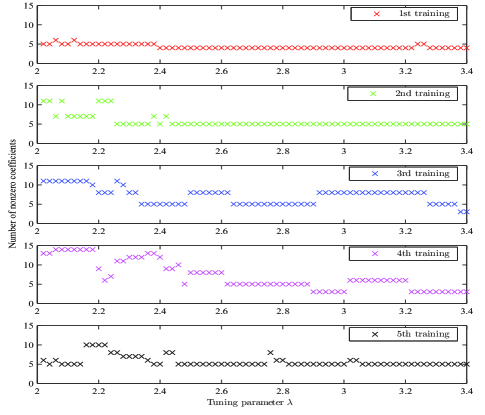
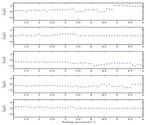
To resolve the training inconsistency, we advocate a generic selective cross validation (SCV) for parameter tuning in sparsity-inducing penalties. First the sparsity algorithm is run on the entire dataset to get a solution path $\hat{\boldsymbol{\beta}}(\lambda_{l})$, $l=1,\cdots,L$. Every estimate $\hat{\boldsymbol{\beta}}(\lambda_{l})$ determines a candidate model with the predictor set given by $nz_{l}=nz(\hat{\boldsymbol{\beta}}(\lambda_{l}))=\{f_{k}\in\mathcal{F}:\hat{\beta}_{k}^{2}+\hat{\beta}_{k+D}^{2}\neq 0\}$. Next, we cross-validate $nz_{l}$ (instead of $\lambda$) to evaluate the goodness-of-fit of each candidate model. In this way, all $\mathpzc K$ trainings are restricted to the same subset of predictors. Concretely, for penalties without $l_{2}$ shrinkage, such as the $l_{0}$-penalty, $\hat{\boldsymbol{\beta}}^{(-\mathpzc{k})}(\lambda_{l})$ is the unpenalized regression estimate fitted on $({\boldsymbol{y}}^{(-\mathpzc{k})},{\boldsymbol{X}}_{nz_{l}}^{(-\mathpzc{k})})$, while for penalties with $l_{2}$ shrinkage, such as the $l_{0}+l_{2}$-penalty, $\hat{\boldsymbol{\beta}}^{(-\mathpzc{k})}(\lambda_{l})$ is the ridge regression estimate fitted on $({\boldsymbol{y}}^{(-\mathpzc{k})},{\boldsymbol{X}}_{nz_{l}}^{(-\mathpzc{k})})$ (cf. Theorem 1), i.e., $\hat{\boldsymbol{\beta}}^{(-\mathpzc{k})}(\lambda_{l})=(({\boldsymbol{X}}_{nz_{l}}^{(-\mathpzc{k})})^{T}{\boldsymbol{X}}_{nz_{l}}^{(-\mathpzc{k})}+\eta\boldsymbol{I})^{T}({\boldsymbol{X}}_{nz_{l}}^{(-\mathpzc{k})})^{T}{\boldsymbol{y}}^{(-\mathpzc{k})}$. Finally, the total SCV error is summarized by $\mbox{SCV}(\lambda_{l})=\sum_{\mathpzc k=1}^{\mathpzc K}\|{\boldsymbol{y}}^{(\mathpzc{k})}-{\boldsymbol{X}}^{(\mathpzc{k})}\hat{\boldsymbol{\beta}}^{(-\mathpzc k)}(\lambda_{l})\|_{2}^{2}$.

Motivated by the work of [37], we add a high-dimensional BIC correction term to define the model comparison criterion: $\mbox{SCV-BIC}(\lambda_{l})=\mbox{SCV}(\lambda_{l})+\mbox{DF}(\hat{\boldsymbol{\beta}}(\lambda_{l}))\log N$, where DF is the degrees of freedom function. When the true signal has a parsimonious representation in the frequency domain, i.e., the number of present frequencies is very small, such a correction is necessary—see [37] for a further theoretical justification. For the $l_{0}$ or $l_{1}$ penalty, DF is approximately the number of nonzero components in the estimate; for the $l_{0}+l_{2}$ penalty, $\mbox{DF}(\hat{\boldsymbol{\beta}}(\lambda_{l}))$ is given by $Tr(({\boldsymbol{X}}_{nz_{l}}^{T}{\boldsymbol{X}}_{nz_{l}}+\eta{\boldsymbol{I}})^{-1}{\boldsymbol{X}}_{nz_{l}}^{T}{\boldsymbol{X}}_{nz_{l}})$ [36]. The optimal estimate $\hat{\boldsymbol{\beta}}_{opt}$ is chosen from the original solution path $\{\hat{\boldsymbol{\beta}}(\lambda_{l})\}_{l=1}^{L}$ by minimizing $\mbox{SCV-BIC}(\lambda_{l})$.

We point out that in SCV, the sparsity algorithm is only required to run on the whole dataset to generate one solution path, while CV needs $\mathpzc K$ such solution paths. SCV is more efficient in computation.

III-E Probabilistic spectra screening

Computational complexity is another major challenge in super-resolution studies. In Algorithm 1, each iteration step involves only matrix-vector multiplications and componentwise thresholding operations. Both have low complexity and can be vectorized. The total number of flops is no more than $(4DN+8D)\Omega$, which is linear in $D$. In our experiments, $\Omega=200$ suffices and thus the complexity of Algorithm 1 is $O(DN)$. (Restricting attention to uniformly sampled data and frequency atoms in the dictionary construction, we can use the Fast Fourier transform (FFT) in computation to reduce the complexity to $O(D\log D)$, as pointed out by an anonymous reviewer, see [39] and Section IV.) On the other hand, with a superbly high resolution dictionary (where $D$ is very large), dimension reduction is still desirable to further reduce the computational cost.

This is indeed possible under the spectral sparsity assumption, where the number of true components is supposed to be much smaller than $N$. One may reduce the dimension from $2D$ to $\vartheta N$ (say $\vartheta=0.5$) before running the formal algorithm. If the $\vartheta N$ candidate predictors are wisely chosen, the truly relevant atoms will be included with high probability and the performance sacrifice in selection/estimation will be mild. Hereinafter, we call $\vartheta$ the candidate ratio. A well designed screening algorithm should not be very sensitive to $\vartheta$ as long as it is reasonably large. Significant decrease in computational time can be achieved after this supervised dimension reduction.

We propose an iterative probabilistic screening by adapting Algorithm 1 for dimension reduction. This has the benefit that the screening principle is consistent with the fitting criterion. We recommend using the hard-ridge thresholding and the associated Algorithm 2 is stated below.

  given ${\boldsymbol{X}}$ (design matrix, normalized), ${\boldsymbol{y}}$ (centered), $\eta$ ($l_{2}$ shrinkage parameter), $\vartheta$ (candidate ratio–ratio of new dimension to sample size), $\omega$ (relaxation parameter), and $\tilde{\Omega}$ (maximum number of iterations). (For simplicity, assume $\vartheta N$ is an integer.)

  1) ${\boldsymbol{X}}\leftarrow{\boldsymbol{X}}/\tau_{0}$, ${\boldsymbol{y}}\leftarrow{\boldsymbol{y}}/\tau_{0}$, with $\tau_{0}\geq\|{\boldsymbol{X}}\|_{2}$ (spectral norm).

  2) Let $j\leftarrow 0$ and ${\boldsymbol{\beta}}^{(0)}$ be an initial estimate say $\boldsymbol{0}$.

  while $\|{\boldsymbol{\beta}}^{(j+1)}-{\boldsymbol{\beta}}^{(j)}\|$ is not small enough or $j\leq\tilde{\Omega}$ do

     3.1) ${\boldsymbol{\xi}}^{(j+1)}\leftarrow(1-\omega){\boldsymbol{\xi}}^{(j)}+\omega({\boldsymbol{\beta}}^{(j)}+{\boldsymbol{X}}^{T}({\boldsymbol{y}}-{\boldsymbol{X}}{\boldsymbol{\beta}}^{(j)}))$ if $j>0$ and ${\boldsymbol{\xi}}^{(j+1)}\leftarrow{\boldsymbol{\beta}}^{(j)}+{\boldsymbol{X}}^{T}({\boldsymbol{y}}-{\boldsymbol{X}}{\boldsymbol{\beta}}^{(j)})$ if $j=0$, and set $m^{(j)}=\vartheta N$; Group form:

     3.2a) $l_{k}^{(j+1)}\leftarrow\sqrt{(\xi_{k}^{(j+1)})^{2}+(\xi_{k+D}^{(j+1)})^{2}}$, $1\leq k\leq D$

     3.2b) Let $\lambda$ be the median of the $m^{(j)}$th largest and ($m^{(j)}+1$)th largest elements in $\{\boldsymbol{l}_{k}^{(j+1)}\}$. For each $k:1\leq k\leq D$, if $l_{k}^{(j+1)}\neq 0$, set $[{\boldsymbol{\beta}}_{k}^{(j+1)},{\boldsymbol{\beta}}_{k+D}^{(j+1)}]\leftarrow[{\xi_{k}^{(j+1)}},{\xi_{k+D}^{(j+1)}}]\Theta_{HR}(l_{k}^{(j+1)};{\lambda},\eta)/l_{k}^{(j+1)}$; set ${\boldsymbol{\beta}}_{k}^{(j+1)}={\boldsymbol{\beta}}_{k+D}^{(j+1)}=0$ otherwise.

     Non-Group form:

     3.2’) ${\boldsymbol{\beta}}^{(j+1)}\leftarrow\Theta_{HR}({\boldsymbol{\xi}}^{(j+1)};{\lambda},\eta)$, where $\lambda$ is the median of the $m^{(j)}$th largest component and the $(m^{(j)}+1)$th largest component of $|{\boldsymbol{\beta}}^{(j+1)}|$;

  end while

  deliver  Remaining dimensions after screening: $\{f\in\mathcal{F}:\|{\boldsymbol{\beta}}_{f}^{(j+1)}\|_{2}\neq 0\}$ (group version) or $\{k:1\leq k\leq 2D,\beta_{k}^{(j+1)}\neq 0\}$ (non-group version).

Algorithm 2 GIST-Screening algorithm.

The differences in comparison to Algorithm 1 lie in (3.2b) and (3.2’), where a dynamic threshold is constructed in performing the hard-ridge thresholding. We next show that this screening version still has convergence guarantee. Similar to Theorem 1, assume $\tau_{0}=1>\|{\boldsymbol{X}}\|_{2}$. Let $G$ be the same energy function constructed in (16) with $P$ given by (11) or (12). For simplicity, suppose $m:=\vartheta N\in\mathbb{N}$. Theorem 3 shows that Algorithm 2 solves an $l_{0}$-constrained problem.

Theorem 3

For any $0<\omega\leq 1$, the sequence of iterates $({\boldsymbol{\beta}}^{(j)},{\boldsymbol{\xi}}^{(j)})$ from Algorithm 2 has the same function value decreasing property (17) for the energy function $G$, and ${\boldsymbol{\beta}}^{(j)}$ satisfies $nz({\boldsymbol{\beta}}^{(j)})\leq m$. In addition, under $\eta>0$ and the no-tie-occurring assumption $\mathfrak{B}$ in Appendix C, the sequence of ${\boldsymbol{\beta}}^{(j)}$ has a unique limit point ${\boldsymbol{\beta}}^{\circ}$ which corresponds to the ridge estimate restricted to ${\boldsymbol{X}}_{nz({\boldsymbol{\beta}}^{\circ})}$ with $|nz({\boldsymbol{\beta}}^{\circ})|\leq m$.

We can use SCV to tune $\eta$ or simply set $\eta$ at a small value (say 1e-2). In practice, the screening can proceed in a progressive fashion to avoid greedy selection: we use a varying sequence of $m^{(j)}$ that decreases to $\vartheta N$ in Step 3.1), and add ‘squeezing’ operations after Step 3.2) or 3.2’): ${\boldsymbol{d}}\leftarrow\{f\in\mathcal{F}:\|{\boldsymbol{\beta}}_{f}^{(j+1)}\|_{2}\neq 0\},{\boldsymbol{\beta}}^{(j+1)}\leftarrow{\boldsymbol{\beta}}^{(j+1)}[{\boldsymbol{d}}],{\boldsymbol{X}}\leftarrow{\boldsymbol{X}}[,{\boldsymbol{d}}]$ (group version), or ${\boldsymbol{d}}\leftarrow\{k:1\leq k\leq 2D,{\boldsymbol{\beta}}_{k}^{(j+1)}\neq 0\},{\boldsymbol{\beta}}^{(j+1)}\leftarrow{\boldsymbol{\beta}}^{(j+1)}[{\boldsymbol{d}}],{\boldsymbol{X}}\leftarrow{\boldsymbol{X}}[,{\boldsymbol{d}}]$ (non-group version). We have found that empirically, the sigmoidal decay cooling schedule $m^{(j)}=\lceil{2D}/(1+\exp(\alpha j))\rceil$ with $\alpha=0.01$ achieves good balance between selection and efficiency.

GIST-Screening works decently in super-resolution spectral analysis seen from the experiments: after dimension reduction the true signal components are included with high probability and the computational cost can be significantly reduced.

An interesting observation is that with ${\boldsymbol{\beta}}^{(0)}=\boldsymbol{0}$, the first iteration step of Algorithm 2 ranks the frequencies based on ${\boldsymbol{X}}^{T}{\boldsymbol{y}}$. In other words, the correlation between the signal ${\boldsymbol{y}}$ and each dictionary atom is examined separately, to determine the candidate dimensions, see [40]. Of course, this type of single frequency analysis is merely marginal and does not amount to joint modeling, the resulting crude ranking not suitable for super resolution problems due to the existence of many correlated frequency predictors. Algorithm 2 iterates and avoids such greediness.

GIST screening is pretty flexible and useful, even if sparsity is not desired. It can be applied at any given value of $\vartheta$ (possibly greater than 1) and yields a meaningful result for super-resolution spectral problems.

III-F GIST framework

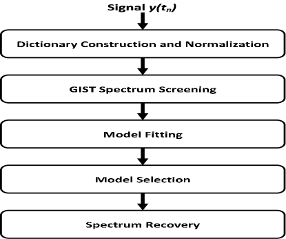
We introduce the complete GIST framework to solve the spectral estimation problem. Fig. 4 shows the flowchart outline.

1. Dictionary Construction and Normalization: We construct an overcomplete dictionary through (2) with sufficiently high resolution. Then standardize the data, by (a) centering ${\boldsymbol{y}}$ and (b) normalizing each predictor column in ${\boldsymbol{X}}$ to have mean 0 and variance 1. After the standardization, all predictors are equally extended in the predictor space.

2. GIST Spectrum Screening: This step can greatly reduce the computational complexity. We perform the iterative probabilistic screening to remove a number of nuisance frequency components and keep $\vartheta N$ candidate predictors with $\vartheta<1$ (say $\vartheta=0.5$) to achieve supervised dimension reduction. See Section III-E for details.

3. Model Fitting: For each given value of the regularization parameter in a predefined grid, run the iterative group-thresholding algorithm developed in Section III-B to obtain a local optimum to (7). All such solutions are collected to form a solution path parameterized by the regularization parameters.

4. Model Selection: An optimal solution $\hat{{\boldsymbol{\beta}}}_{opt}$ is selected from the solution path based on a data-resampling version of high-dimensional BIC (Section III-D).

5. Spectrum Recovery: The signal can be reconstructed from the coefficient estimate. The amplitudes are estimated by $A(f_{k})=\sqrt{\hat{{\boldsymbol{\beta}}}_{opt,k}^{2}+\hat{{\boldsymbol{\beta}}}_{opt,D+k}^{2}}$, $1\leq k\leq D$.

Figure 4: The flowchart of the GIST framework for solving the spectral estimation problem.

IV Experiments

We conduct simulation experiments to show the performance of GIST fitting Algorithm 1 in sparse spectral estimation, and the power of GIST screening Algorithm 2 in fast computation (with little performance loss in frequency detection).

IV-A Simulation setup

Consider a discrete real-valued signal given by

$$y(t_{n})=\sum_{f_{k}\in nz^{*}}A_{k}\cos(2\pi f_{k}t_{n}+\phi_{k})+e(t_{n}),$$ (22)

where $e(t_{n})$ is white Gaussian noise with variance $\sigma^{2}$. $N=100$ training samples are observed at time $t_{n}=n$, $1\leq n\leq N$. The spectrum frequency dictionary is constructed by setting the maximum frequency $f_{\max}=0.5$ Hz, resolution level $\delta=0.02Hz$, and the number of frequency bins $D=f_{\max}/\delta=250$ (and thus $500$ atoms). Using the notation in Section III-C (cf. (19)), we set $nz^{*}=\{0.248,0.25,0.252,0.398,0.4\}$, the associated amplitudes $A_{k}$ and phases $\phi_{k}$ given by $[2,4,3,3.5,3]$ and $[\pi/4,\pi/6,\pi/3,\pi/5,\pi/2]$, respectively. We vary the noise level by $\sigma^{2}=1,4,8$ to study the algorithmic performance with respect to SNR.

Due to random fluctuation, reporting frequency identification for one particular simulation dataset is meaningless. Instead, we simulated each model 50 times to enhance stability, where at each run $e(t_{n})$ are i.i.d. following $\mathcal{N}(0,\sigma^{2})$.

Our simulations were performed in MATLAB R2010b and Win7 Professional 32-bit OS, on a desktop with an Intel(R) Core(TM)2 Quad 2.66 GHz processor and 4GB memory.

IV-B Experimental Results

IV-B1 Comparison with some existing methods

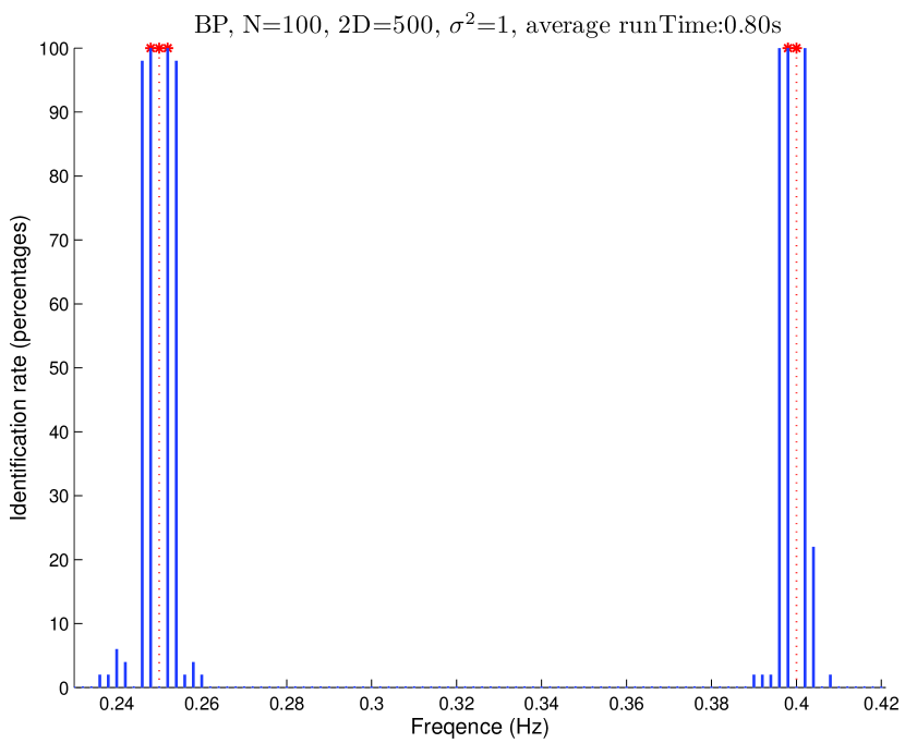
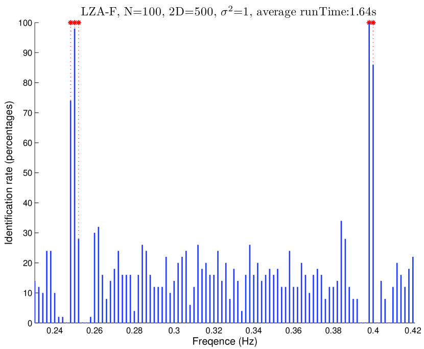
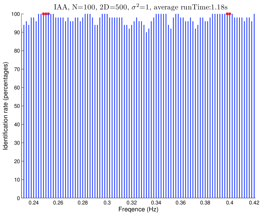
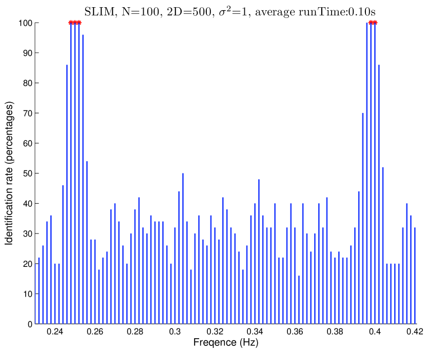
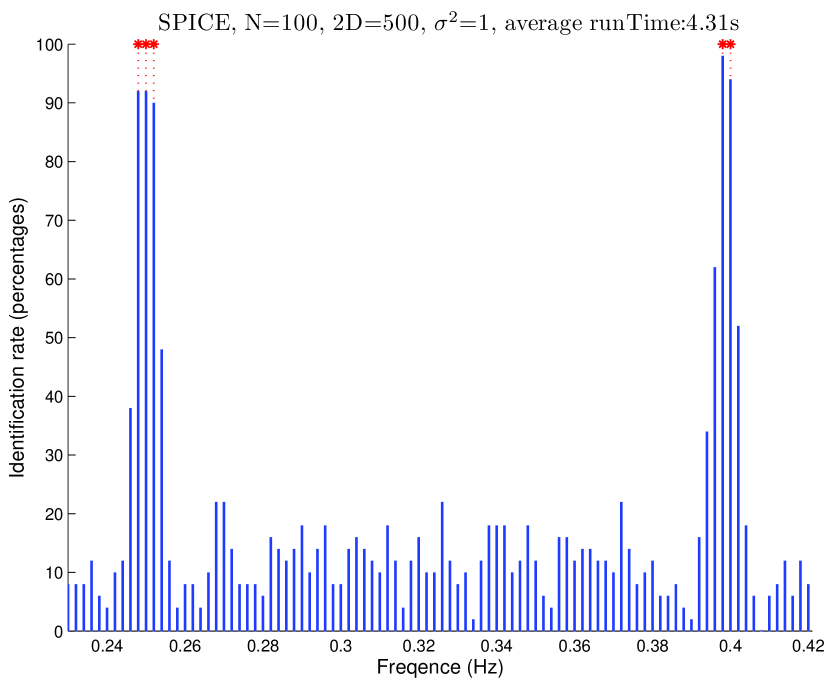
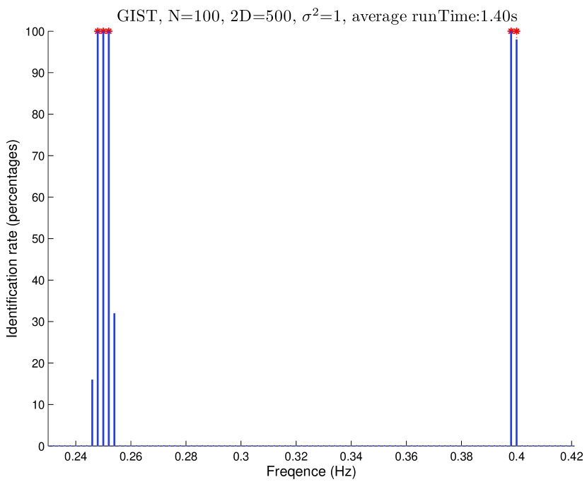
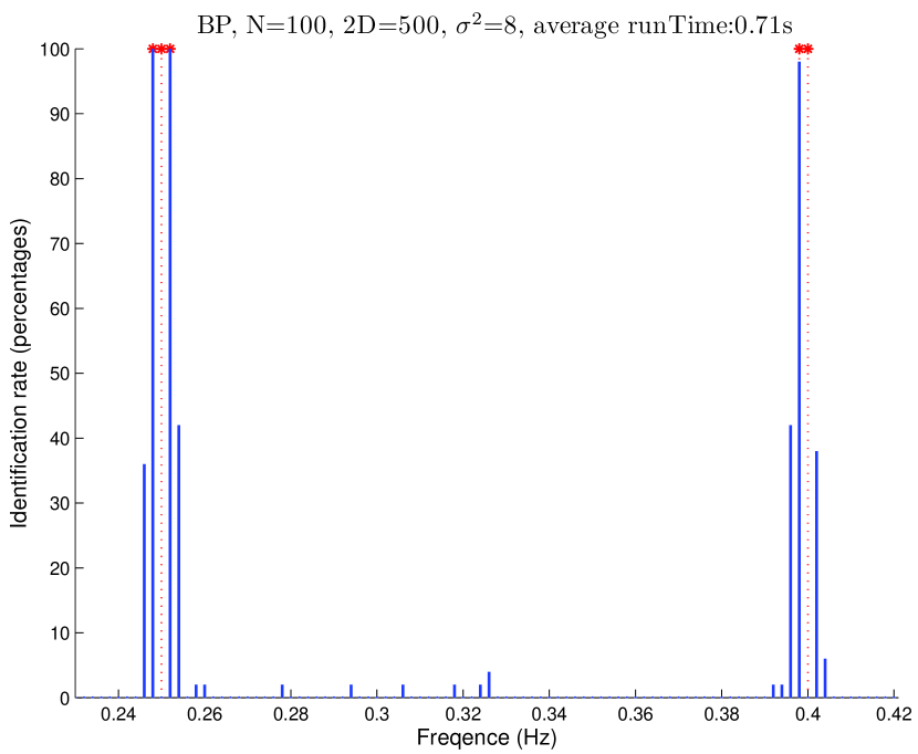
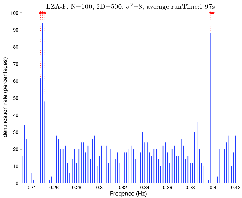
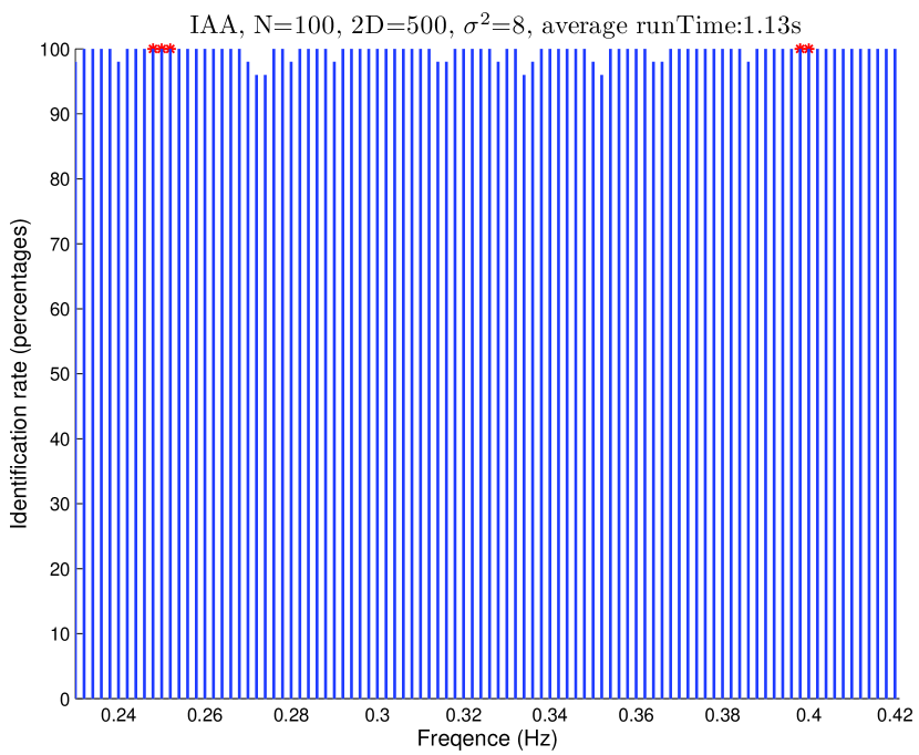
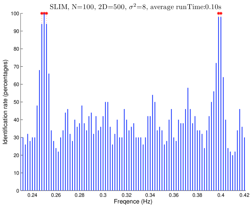
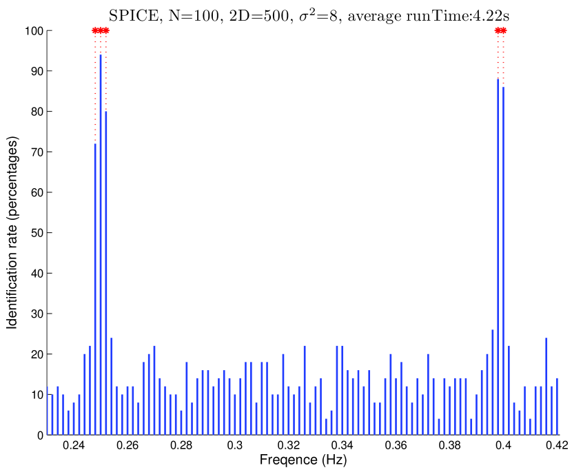
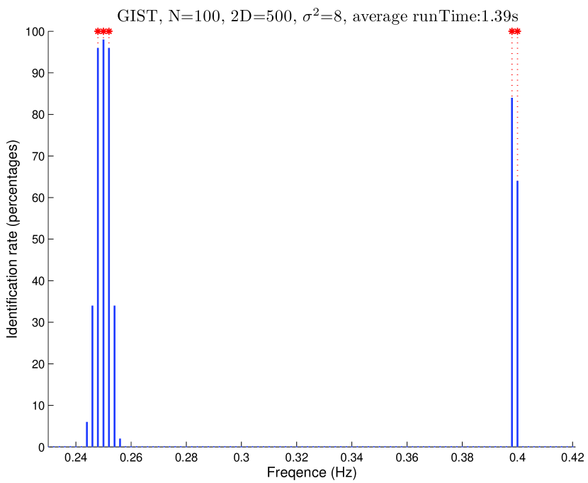
To compare with the advocated group hard-ridge GIST (or GIST for short), we implemented BP [6], IAA-APES (or IAA for short) [41], SPICE [42], LZA-F [14], CG-SLIM (or SLIM for short) [39]. To make a fair and realistic comparison, we used a common stopping criterion: the number of iterations reaches $200$ or the change in ${\boldsymbol{\beta}}$ is less than 1e-4. In GIST, we set $\vartheta=0.25$ to give the cardinality bound in screening, and used SCV-BIC for parameter tuning. The algorithmic parameters in the other methods took default values suggested in the literature. (For example, the $q$ parameter in SLIM is chosen to be $1$, as recommended and used in the numerical examples of [39].) Figs. 5 and 6 show the frequency identification rates in 50 simulation runs for each of the methods under $\sigma^{2}=1$ and $\sigma^{2}=8$, respectively. That is, given each algorithm, we plotted the percentage of identifying $f_{k}$ or $\hat{\boldsymbol{\beta}}_{f_{k}}\neq 0$ in all runs, for every $f_{k}$ in the dictionary. The blue solid lines show such identification rates, while the red dotted lines (with star marks at $100\%$) label the true frequencies. The plot for $\sigma^{2}=4$ is similar to Fig. 6; we do not show it here due to the page limit. We also included the running time (averaged over 50 runs) in Table I to reflect the computational cost.

(a) BP

(b) LZA-F

(c) IAA

(d) SLIM

(e) SPICE

(f) GIST

Figure 5: Frequency identification rates with $\sigma^{2}=1$ in 50 simulation runs, using BP, LZA-F, IAA, SLIM, SPICE, and GIST.

(a) BP

(b) LZA-F

(c) IAA

(d) SLIM

(e) SPICE

(f) GIST

Figure 6: Frequency identification rates with $\sigma^{2}=8$ in 50 simulation runs, using BP, LZA-F, IAA, SLIM, SPICE, and GIST.

TABLE I: Average runtime in seconds of different algorithms, with varying values of $\sigma^{2}$ at $1$, $4$, and $8$.

	$\sigma^{2}=1$	$\sigma^{2}=4$	$\sigma^{2}=8$
BP	0.80	0.72	0.71
LZA-F	1.64	1.88	1.97
[1pt/2pt] IAA	1.18	1.09	1.13
SLIM	3.77	3.71	3.70
SLIM with FFT	0.10	0.10	0.10
[1pt/2pt] SPICE	4.31	4.23	4.22
GIST	1.40	1.40	1.39

IAA, SPICE, LZA-F, and SLIM are not capable of producing inherently sparse estimates. One must make a somewhat ad-hoc choice of the cutoff value $\tau$ to discern the present frequencies. We set $\tau=1e-2$ in performing such post-truncation. It behaved better than $\tau=1e-3$ or $\tau=1e-4$ in experimentation (which gave similar yet worse detection performance).

BP, though super fast, missed the frequency components at $0.25$ and $0.4$ all the time. An improvement is offered by the CG-SLIM which makes use of the group $l_{1}$ regularization. In [39], CG-SLIM is recommended to run for only 20 iteration steps (whereas the simulated signals there had very mild noise contamination, with $\sigma^{2}=0.001$). Here, we increased the maximum number of iterations to 200 for better identification, without sacrificing much efficiency. Otherwise CG-SLIM gave much poorer spectrum recovery in experiments.

SLIM is free of parameter tuning, because from a Bayesian perspective SLIM estimates the noise variance $\sigma^{2}$ in addition to the coefficient vector ${\boldsymbol{\beta}}$. Unfortunately, we found all the variance estimates from SLIM were severely biased downward—for example, for $\sigma^{2}=8$, the mean $\hat{\sigma}^{2}$ in 50 runs is about $3e-5$. This is perhaps the reason why SLIM failed in super-resolution recovery: with such a small $\sigma^{2}$ estimate, the threshold level tends to be very low, and thus SLIM always overselects. Seen from the figures, SLIM results in many spurious frequencies, some arising in more than 60 percent of the datasets. IAA is even worse and does not seem to have the ability to super-resolve.

It is observed that LZA-F may seriously mask the true components. In addition, with moderate/large noise contamination, we found that LZA-F may be unstable and produce huge errors. Because the design of LZA-F is to approximate the $l_{0}$ regularization, we substituted the hard-thresholding for $\Theta$ in GIST, which solves the exact $l_{0}$-penalized problem. However, the high miss rates of the $l_{0}$-type regularization are still commonly seen, and the resulting models are often over-sparse. To give an explanation of this under-selection, notice that the $l_{0}$ regularization either kills or keeps, thereby offering no shrinkage at all for nonzero coefficients. To attain the appropriate extent of shrinkage especially when the noise is not too small, it has to kill more predictors than necessary. As a conclusion, inappropriate nonconvex penalties may seriously mask true signal components.

In our experiments, SPICE performs well. GIST is much better and shows more concentrated signal power at the true frequencies. It produces very few spurious frequencies, and in terms of computation, it is much more efficient than SPICE (Table I). GIST adapts to SNR and is both stable and scalable.

Finally, a recent proposal of using the FFT for matrix-vector multiplication [39] was shown to be very effective: for SLIM, the average running time dropped from about 3.7 seconds to 0.1 seconds. The computational trick can be applied to all of the methods discussed here. However, it restricts to uniformly sampled data with Fourier dictionaries. We did not use the FFT implementation for the other methods. (GIST algorithms and analyses are general and do not have such restrictions, see Section III and Section V.)

IV-B2 Probabilistic spectral screening

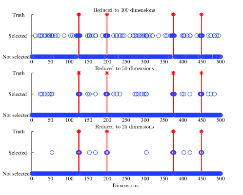
We examine the performance of the GIST-screening Algorithm 2 in this experiment. The candidate ratio $\vartheta$ determines the dimensions ($\vartheta N$) of the reduced predictor space. Therefore, the lower the value of $\vartheta$, the more efficient the computation, but also the higher the risk of mistakenly removing some true components. Our screening technique turns out to be pretty successful: even if we choose $\vartheta N$ to be as small as $25$ (which can be even lower), it never misses any true frequency component. Fig. 8 shows the frequency location of $100$, $50$, and $25$ remaining atoms, respectively, in GIST screening. The selected frequencies are non-uniform, and the density near the true spectra is much higher.

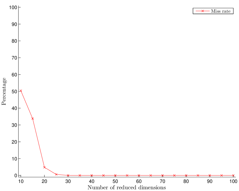
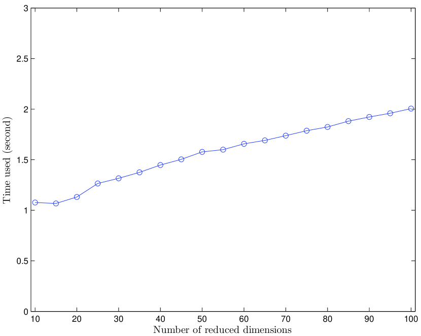
Next, we make a much more challenging problem by modifying the signal to have 10 present frequency components at $0.24,0.242,\ldots,0.282$ and large noise variance $\sigma^{2}=10$. Fig. 8 shows both the detection miss rates and the computation time, averaged over 50 runs. The miss rate is the mean of $|\{i:\beta_{i}^{*}\neq 0,\hat{\beta}_{i}=0\}|/|\{i:\beta_{i}^{*}\neq 0\}|$ in all simulations, where $|\cdot|$ is the cardinality of a set. The plotted time is the total running time of both GIST screening and model fitting and selection. The empirical experience is that GIST-screening is safe when $\vartheta N$ is roughly 3 times greater than the number of truly relevant atoms. It reduces the computation complexity significantly with little performance lost.

Figure 7: Locations of the remaining frequency atoms after GIST screening with $\vartheta N=100,50,25$. The true frequencies are indicated by red lines and stars.

Figure 8: Performance of GIST screening on a hard problem with 10 present frequency components and large noise variance $\sigma^{2}=10$. The left panel shows the miss rates, while the right panel shows the total computational time (including the GIST fitting time thereafter); both $x$-axes represent $\vartheta N$, the dimensions to be kept after screening.

IV-B3 Misspecified resolution level

In super-resolution spectral selection, the frequency resolution level $\delta$ used in dictionary construction is customized by users. This requires the knowledge of a lower bound on frequency spacing. We are particularly interested in the performance of GIST when $\delta$ is misspecified in reference to the truth.

In this experiment, we set the signal frequencies at $0.2476$, $0.2503$, $0.2528$, $0.3976$, $0.4008$, with amplitudes $A_{k}$ and phases $\phi_{k}$ unchanged. Clearly, the ideal frequency resolution to resolve this signal should be no more than $0.0001$ Hz.

We chose $\delta=0.002$, 20 times as large as the required resolution. The results are nearly identical to Figs. (5(f)), (6(f)) (not shown due to space limitation). The crude resolution specification makes GIST unable to recover the true frequencies. On the other hand, the most frequently identified frequencies are $0.248$, $0.25$, $0.252$, $0.398$, $0.4$, and a comparison shows that this is the best approximation in the given frequency grid. (For example, $0.398$Hz is the closest frequency in the grid $\{0,0.02,\cdots,0.396,0.398,\cdots,0.5\}$ to $0.3976$Hz.) This phenomenon is also seen in many other experiments: GIST gives the best possible identification to approximate the true frequencies, with the quantization error determined by the resolution level.

V Conclusions

We have presented a sparsity-based GIST framework to tackle the super-resolution challenge in spectral estimation. It is able to handle nonconvex penalties and take the pairing structure of sine and cosine atoms into account in regularizing the model. The $l_{0}+l_{2}$ type hard-ridge penalty was shown to be able to dramatically improve the popular convex $l_{1}$ penalty as well as the nonconvex $l_{0}$ penalty. Its variant, the iterative probabilistic spectrum screening, can be used for supervised dimension reduction and fast computation. In parameter tuning, the SCV criterion overcomes the training inconsistency issue of the plain CV and is much more computationally efficient. GIST can be applied to unevenly sampled signals (in which case the sampling time sequence $\{t_{n}\}_{1\leq n\leq N}$ is not uniform) with guaranteed convergence (cf. Theorem 1 and Theorem 3).

It is worth mentioning that in our algorithm design and theoretical analyses, the only use of the Fourier frequency dictionary was to extract the atom grouping manner. Our methodology carries over to any type of dictionary as arising in signal processing, wavelets, and statistics. For example, although we focused on real-valued signals in the paper, for complex-valued signals, say, ${\boldsymbol{y}}=[y(t_{n})]\in\mathbb{C}^{N\times 1}$ observed at $t_{n}$ ($1\leq n\leq N$) and the candidate frequency grid given by $f_{k}$ ($1\leq k\leq D$), a complex dictionary ${\boldsymbol{X}}$ can be constructed as $[\exp(i2\pi f_{k}t_{n})]\in\mathbb{C}^{N\times D}$ in place of (2), with ${\boldsymbol{\beta}}=[\beta_{1},\cdots,\beta_{D}]^{T}\in\mathbb{C}^{D}$. The group penalized model then minimizes ${1\over 2}\|{\boldsymbol{y}}-\alpha-{\boldsymbol{X}}{\boldsymbol{\beta}}\|_{2}^{2}+\sum_{k=1}^{D}P\left(\|\beta_{k}\|_{2};\lambda\right)$ where $\|\beta_{k}\|_{2}=\sqrt{\mbox{Re}(\beta_{k})^{2}+\mbox{Im}(\beta_{k})^{2}}$, simply the complex norm of $\beta_{k}$. It is straightforward to extend all our algorithms and analyses to this problem. On the other hand, for real-valued signals, the formulation using the sine-cosine predictor matrix in (2) does not involve any imaginary/complex number processing in implementation.

Some future research topics include the extension of GIST to non-Gaussian and/or multivariate signals.

Appendix A Proof of Theorem 1

We show the result for the group form only. The proof for the non-group form is similar and simpler. The following continuity assumption is made throughout the proof:

Assumption $\mathfrak{A}$: $\vec{\Theta}$ is continuous at any point in the closure of $\{{\boldsymbol{\xi}}^{(j)}\}$.
For continuous thresholding rules such as soft-thresholding, this regularity condition always holds. Practically used thresholding rules (such as hard-thresholding) have few discontinuity points and such discontinuities rarely occur in any real application. For $\omega=1$, see [28] for the proof details. In the following, we assume $0<\omega<1$.

Note that $G$ is quadratic and convex in ${\boldsymbol{\beta}}$, ${\boldsymbol{\xi}}$, and ${\boldsymbol{\zeta}}$, but possibly nonconvex and nonsmooth in ${\boldsymbol{\gamma}}$.

Lemma A.1

Given an arbitrary thresholding rule $\Theta$, let $P$ be any function satisfying

$$P(\theta;\lambda)-P(0;\lambda)=P_{\Theta}(\theta;\lambda)+q(\theta;\lambda)$$

where $P_{\Theta}(\theta;\lambda)\triangleq\int_{0}^{|\theta|}(\sup\{s:\Theta(s;\lambda)\leq u\}-u)\,\mathrm{d}u$, $q(\theta;\lambda)$ is nonnegative and $q(\Theta(t;\lambda))=0$ for all $t$. Then, the minimization problem

$$\min_{{\boldsymbol{\beta}}}\frac{1}{2}\|{\boldsymbol{y}}-{\boldsymbol{\beta}}\|_{2}^{2}+P(\|{\boldsymbol{\beta}}\|_{2};\lambda)$$

has a unique optimal solution given by $\hat{\boldsymbol{\beta}}=\vec{\Theta}({\boldsymbol{y}};\lambda)$ for every ${\boldsymbol{y}}$ provided that $\Theta(\cdot;\lambda)$ is continuous at $\|{\boldsymbol{y}}\|_{2}$.

See [28] for its proof.

Given ${\boldsymbol{\beta}}$ and ${\boldsymbol{\xi}}$, the problem of minimizing $G$ over $({\boldsymbol{\gamma}},{\boldsymbol{\zeta}})$ can be simplified to (detail omitted)

$$\min_{{\boldsymbol{\gamma}}}\frac{1}{2}\|{\boldsymbol{\gamma}}-\omega({\boldsymbol{I}}-{\boldsymbol{\Sigma}}){\boldsymbol{\beta}}-\omega{\boldsymbol{X}}^{T}{\boldsymbol{y}}-(1-\omega){\boldsymbol{\xi}}\|_{2}^{2}+P({\boldsymbol{\gamma}};\lambda),$$

and

$$\min_{{\boldsymbol{\zeta}}}\frac{1}{2}\frac{1-\omega}{\omega}[{\boldsymbol{\zeta}}-\omega({\boldsymbol{I}}-{\boldsymbol{\Sigma}}){\boldsymbol{\beta}}-\omega{\boldsymbol{X}}^{T}{\boldsymbol{y}}-(1-\omega){\boldsymbol{\xi}}]^{T}({\boldsymbol{I}}-{\boldsymbol{\Sigma}})^{-1}[{\boldsymbol{\zeta}}-\omega({\boldsymbol{I}}-{\boldsymbol{\Sigma}}){\boldsymbol{\beta}}-\omega{\boldsymbol{X}}^{T}{\boldsymbol{y}}-(1-\omega){\boldsymbol{\xi}}].$$

Based on Lemma A.1, the optimal solutions are

$$\begin{cases}{\boldsymbol{\gamma}}_{opt}&=\vec{\Theta}(\omega({\boldsymbol{I}}-{\boldsymbol{\Sigma}}){\boldsymbol{\beta}}+\omega{\boldsymbol{X}}^{T}{\boldsymbol{y}}+(1-\omega){\boldsymbol{\xi}};\lambda)\\ {\boldsymbol{\zeta}}_{opt}&=\omega({\boldsymbol{I}}-{\boldsymbol{\Sigma}}){\boldsymbol{\beta}}+\omega{\boldsymbol{X}}^{T}{\boldsymbol{y}}+(1-\omega){\boldsymbol{\xi}}.\end{cases}$$

Therefore, we obtain

$$G({\boldsymbol{\beta}}^{(j+1)},{\boldsymbol{\xi}}^{(j+1)},{\boldsymbol{\beta}}^{(j)},{\boldsymbol{\xi}}^{(j)};\lambda)\leq G({\boldsymbol{\beta}}^{(j)},{\boldsymbol{\xi}}^{(j)},{\boldsymbol{\beta}}^{(j)},{\boldsymbol{\xi}}^{(j)};\lambda)-\frac{1-\omega}{2\omega}({\boldsymbol{\xi}}^{(j+1)}-{\boldsymbol{\xi}}^{(j)})^{T}({\boldsymbol{I}}-{\boldsymbol{\Sigma}})^{-1}({\boldsymbol{\xi}}^{(j+1)}-{\boldsymbol{\xi}}^{(j)}).$$ (23)

On the other hand, given ${\boldsymbol{\gamma}}$ and ${\boldsymbol{\zeta}}$, $G$ can be expressed as a quadratic form in ${\boldsymbol{\beta}}$ that is positive definite. The same fact holds for ${\boldsymbol{\xi}}$. It can be computed that

$$\begin{cases}\nabla G_{{\boldsymbol{\beta}}}=\omega({\boldsymbol{I}}-{\boldsymbol{\Sigma}})({\boldsymbol{\beta}}-{\boldsymbol{\gamma}})+(1-\omega)({\boldsymbol{\xi}}-{\boldsymbol{\zeta}})\\ \nabla G_{{\boldsymbol{\xi}}}=\frac{1-\omega}{\omega}({\boldsymbol{I}}-{\boldsymbol{\Sigma}})^{-1}[\omega({\boldsymbol{I}}-{\boldsymbol{\Sigma}})({\boldsymbol{\beta}}-{\boldsymbol{\gamma}})+(1-\omega)({\boldsymbol{\xi}}-{\boldsymbol{\zeta}})],\end{cases}$$

from which it follows that $G$ can be written as $\frac{1}{2}[\omega({\boldsymbol{I}}-{\boldsymbol{\Sigma}})({\boldsymbol{\beta}}-{\boldsymbol{\gamma}})+(1-\omega)({\boldsymbol{\xi}}-{\boldsymbol{\zeta}})]^{T}\omega^{-1}({\boldsymbol{I}}-{\boldsymbol{\Sigma}})^{-1}[\omega({\boldsymbol{I}}-{\boldsymbol{\Sigma}})({\boldsymbol{\beta}}-{\boldsymbol{\gamma}})+(1-\omega)({\boldsymbol{\xi}}-{\boldsymbol{\zeta}})]$ in addition to the terms involving only ${\boldsymbol{\gamma}}$ and ${\boldsymbol{\zeta}}$. Hence ${\boldsymbol{\beta}}_{opt}={\boldsymbol{\beta}}$ and ${\boldsymbol{\xi}}_{opt}={\boldsymbol{\zeta}}$ (though not unique) achieve the minimum. We obtain $G({\boldsymbol{\beta}}^{(j+1)},{\boldsymbol{\xi}}^{(j+1)},{\boldsymbol{\beta}}^{(j+1)},{\boldsymbol{\xi}}^{(j+1)};\lambda)\leq G({\boldsymbol{\beta}}^{(j+1)},{\boldsymbol{\xi}}^{(j+1)},{\boldsymbol{\beta}}^{(j)},{\boldsymbol{\xi}}^{(j)};\lambda)-\frac{1}{2\omega}[\omega({\boldsymbol{I}}-{\boldsymbol{\Sigma}})({\boldsymbol{\beta}}^{(j)}-{\boldsymbol{\beta}}^{(j+1)})+(1-\omega)({\boldsymbol{\xi}}^{(j)}-{\boldsymbol{\xi}}^{(j+1)})]^{T}({\boldsymbol{I}}-{\boldsymbol{\Sigma}})^{-1}[\omega({\boldsymbol{I}}-{\boldsymbol{\Sigma}})({\boldsymbol{\beta}}^{(j)}-{\boldsymbol{\beta}}^{(j+1)})+(1-\omega)({\boldsymbol{\xi}}^{(j)}-{\boldsymbol{\xi}}^{(j+1)})].$ Combining this with (23) yields (17).

Assume a subsequence ${\boldsymbol{\beta}}^{(j_{l})}\rightarrow{\boldsymbol{\beta}}^{\circ}$ as $l\rightarrow\infty$. Because

$$G({\boldsymbol{\beta}}^{(j_{l})},{\boldsymbol{\xi}}^{(j_{l})},{\boldsymbol{\beta}}^{(j_{l})},{\boldsymbol{\xi}}^{(j_{l})})-G({\boldsymbol{\beta}}^{(j_{l}+1)},{\boldsymbol{\xi}}^{(j_{l}+1)},{\boldsymbol{\beta}}^{(j_{l}+1)},{\boldsymbol{\xi}}^{(j_{l}+1)})\longrightarrow 0,$$

we have ${\boldsymbol{\xi}}^{(j_{l})}-{\boldsymbol{\xi}}^{(j_{l}+1)}\rightarrow 0$ and thus $({\boldsymbol{\beta}}^{(j_{l})}-{\boldsymbol{\beta}}^{(j_{l}+1)})\rightarrow 0$. That is, $(1-\omega){\boldsymbol{\xi}}^{(j_{l})}+\omega({\boldsymbol{\beta}}^{(j_{l})}+{\boldsymbol{X}}^{T}({\boldsymbol{y}}-{\boldsymbol{X}}{\boldsymbol{\beta}}^{(j_{l})}))-{\boldsymbol{\xi}}^{(j_{l})}\rightarrow 0$ and $\vec{\Theta}({\boldsymbol{\xi}}^{(j_{l})};\lambda)-{\boldsymbol{\beta}}^{(j_{l})}\rightarrow 0$. From ${\boldsymbol{X}}^{T}({\boldsymbol{y}}-{\boldsymbol{X}}{\boldsymbol{\beta}}^{(j_{l})})-{\boldsymbol{\xi}}^{(j_{l})}\rightarrow 0$ and the continuity assumption, ${\boldsymbol{\beta}}^{\circ}$ is a group $\Theta$-estimate satisfying (13), and $\lim_{j\rightarrow\infty}G({\boldsymbol{\beta}}^{(j_{l})},{\boldsymbol{\xi}}^{(j_{l})},{\boldsymbol{\beta}}^{(j_{l})},{\boldsymbol{\xi}}^{(j_{l})})=F({\boldsymbol{\beta}}^{\circ})$.

Appendix B Proof of Theorem 2

Recall that $\mathcal{F}$ denotes the frequency set covered by the dictionary ${\boldsymbol{X}}$ and we assume all column norms of ${\boldsymbol{X}}$ are $\sqrt{N}$ (or the diagonal entries of ${\boldsymbol{\Sigma}}={\boldsymbol{X}}^{T}{\boldsymbol{X}}$ are equal to $N$).

Applying Theorem 1, we can characterize any group $l_{1}$ estimate $\hat{\boldsymbol{\beta}}$ from Algorithm 1 by

$$\hat{\boldsymbol{\beta}}=\vec{\Theta}(\hat{\boldsymbol{\beta}}+{\boldsymbol{X}}^{T}{\boldsymbol{y}}/\tau_{0}^{2}-{\boldsymbol{\Sigma}}\hat{\boldsymbol{\beta}}/\tau_{0}^{2};\lambda)$$ (24)

with $\Theta$ being the soft-thresholding function. Let ${\boldsymbol{s}}={\boldsymbol{s}}({\boldsymbol{\beta}})$ denote a function of ${\boldsymbol{\beta}}$ satisfying

$$\|{\boldsymbol{s}}_{{f}}\|_{2}\leq 1,\forall f\in z({\boldsymbol{\beta}}),\ {\boldsymbol{s}}_{{f}}={\boldsymbol{\beta}}_{f}/\|{\boldsymbol{\beta}}_{f}\|_{2},\forall f\in nz({\boldsymbol{\beta}}),$$ (25)

and ${\boldsymbol{s}}({\boldsymbol{\beta}}_{f}):=[{\boldsymbol{s}}({\boldsymbol{\beta}})]_{f}$. We have $\|{\boldsymbol{s}}({\boldsymbol{\beta}}_{f})\|_{2}\leq 1$, $\forall f\in\mathcal{F}$. (In the group $l_{1}$ case, ${\boldsymbol{s}}$ is a subgradient of $\sum_{f\in\mathcal{F}}\|{\boldsymbol{\beta}}_{f}\|_{2}$.) Then (24) reduces to $\hat{\boldsymbol{\beta}}+\lambda{\boldsymbol{s}}(\hat{\boldsymbol{\beta}},\lambda)=\hat{\boldsymbol{\beta}}+{\boldsymbol{X}}^{T}{\boldsymbol{y}}/\tau_{0}^{2}-{\boldsymbol{\Sigma}}\hat{\boldsymbol{\beta}}/\tau_{0}^{2}$ or

$${\boldsymbol{\Sigma}}\hat{\boldsymbol{\beta}}={\boldsymbol{X}}^{T}{\boldsymbol{y}}-\lambda\tau_{0}^{2}{\boldsymbol{s}}(\hat{\boldsymbol{\beta}}),$$ (26)

for some ${\boldsymbol{s}}$ satisfying (25).

Lemma B.1

Assume ${\boldsymbol{\Sigma}}_{{nz^{*}}}$ is nonsingular. Then (26) is equivalent to

$$\begin{cases}{\boldsymbol{S}}_{{z^{*}}}\hat{\boldsymbol{\beta}}_{{z^{*}}}={\boldsymbol{X}}_{z^{*}}^{{}^{\prime}T}\boldsymbol{e}+\lambda\tau_{0}^{2}{\boldsymbol{\Sigma}}_{{z^{*}},{nz^{*}}}{\boldsymbol{\Sigma}}_{{nz^{*}}}^{-1}{\boldsymbol{s}}(\hat{\boldsymbol{\beta}}_{{nz^{*}}})-\lambda\tau_{0}^{2}{\boldsymbol{s}}(\hat{\boldsymbol{\beta}}_{{z^{*}}})\\ \hat{\boldsymbol{\beta}}_{{nz^{*}}}={\boldsymbol{\beta}}_{{nz^{*}}}^{*}+{\boldsymbol{\Sigma}}_{{nz^{*}}}^{-1}({\boldsymbol{X}}_{{nz^{*}}}^{T}{\boldsymbol{e}}-\lambda\tau_{0}^{2}{\boldsymbol{s}}(\hat{\boldsymbol{\beta}}_{{nz^{*}}}))-{\boldsymbol{\Sigma}}_{{nz^{*}}}^{-1}{\boldsymbol{\Sigma}}_{{z^{*}},{nz^{*}}}^{T}\hat{\boldsymbol{\beta}}_{{z^{*}}}\end{cases}$$ (27)

where ${\boldsymbol{S}}_{{z^{*}}}:={\boldsymbol{\Sigma}}_{{z^{*}}}-{\boldsymbol{\Sigma}}_{{z^{*}},{nz^{*}}}{\boldsymbol{\Sigma}}_{{nz^{*}}}^{-1}{\boldsymbol{\Sigma}}_{{nz^{*}},{z^{*}}}$, and ${\boldsymbol{X}}_{z^{*}}^{{}^{\prime}T}:={\boldsymbol{X}}_{{z^{*}}}^{T}-{\boldsymbol{\Sigma}}_{{{z^{*}}},{{nz^{*}}}}{\boldsymbol{\Sigma}}_{{nz^{*}}}^{-1}{\boldsymbol{X}}_{{nz^{*}}}^{T}$.

The proof details are given in [32].

Lemma B.2

Suppose $\left[\begin{array}[]{c}z_{1}\\ z_{2}\end{array}\right]\sim N\left(\left[\begin{array}[]{c}0\\ 0\end{array}\right],{\boldsymbol{V}}\right)$, where ${\boldsymbol{V}}$ is a correlation matrix. Then for any $M$, $P(z_{1}^{2}+z_{2}^{2}>M^{2})\leq P(\xi>M^{2}/2)$ with $\xi\sim\chi^{2}(2)$.

From $\|{\boldsymbol{V}}\|_{2}\leq\|{\boldsymbol{V}}\|_{F}\leq 2$, $2{\boldsymbol{I}}-{\boldsymbol{V}}$ is positive semi-definite. Let $z_{1}^{\prime}$, $z_{2}^{\prime}$ be independent standard Gaussian random variables. We get $P(z_{1}^{2}+z_{2}^{2}>M^{2})\leq P((z_{1}^{\prime}\sqrt{2})^{2}+(z_{2}^{\prime}\sqrt{2})^{2}>M^{2})=P(\xi>M^{2}/2)$ from Anderson’s inequality [43].

Lemma B.3

Suppose $\xi\sim\chi^{2}(2)$. Then for any $M$, $P(\xi>2M^{2})\leq M^{2}e^{-(M^{2}-1)}$.

See, e.g., [44] for a proof of this $\chi^{2}$ tail bound.

Let ${\boldsymbol{X}}_{f}^{{}^{\prime}T}={\boldsymbol{X}}_{{f}}^{T}-{\boldsymbol{\Sigma}}_{{{f}},{{nz^{*}}}}{\boldsymbol{\Sigma}}_{{nz^{*}}}^{-1}{\boldsymbol{X}}_{{nz^{*}}}^{T}$, $\forall f\in z^{*}$. From Lemma B.1, we have $P_{1}\geq P(A\cap V)$, with $A:=\{\|{\boldsymbol{X}}_{{f}}^{{}^{\prime}T}{\boldsymbol{e}}+\lambda\tau_{0}^{2}{\boldsymbol{\Sigma}}_{{f},{nz^{*}}}{\boldsymbol{\Sigma}}_{{nz^{*}}}^{-1}{\boldsymbol{s}}(\hat{\boldsymbol{\beta}}_{nz^{*}})\|_{2}\leq\lambda\tau_{0}^{2},\forall{\boldsymbol{s}}\mbox{ satisfying \eqref{s-def}},\forall f\in z^{*}\}$, $V:=\{\|[{\boldsymbol{\Sigma}}_{{nz^{*}}}^{-1}{\boldsymbol{X}}_{{nz^{*}}}^{T}{\boldsymbol{e}}]_{f}\|_{2}+\lambda\tau_{0}^{2}\|[{\boldsymbol{\Sigma}}_{{nz^{*}}}^{-1}{\boldsymbol{s}}(\hat{\boldsymbol{\beta}}_{nz^{*}})]_{f}\|_{2}<\left\|{\boldsymbol{\beta}}_{f}^{*}\right\|_{2},\forall{\boldsymbol{s}}\mbox{ satisfying \eqref{s-def}},\forall f\in nz^{*}\}.$ Therefore, $1-P_{1}\leq P(A^{c}\cup V^{c})\leq P(A^{c})+P(V^{c})$.

From the definition of $\kappa$, $\|{\boldsymbol{\Sigma}}_{{f},{nz^{*}}}{\boldsymbol{\Sigma}}_{{nz^{*}}}^{-1}{\boldsymbol{s}}(\hat{\boldsymbol{\beta}}_{nz^{*}})\|_{2}\leq\kappa\sqrt{p_{nz^{*}}}\|{\boldsymbol{\Sigma}}_{nz^{*}}^{-1}\|_{2}N\sqrt{p_{nz^{*}\cdot 1}}=\kappa p_{nz^{*}}/\mu$, $\forall f\in z^{*}$. It follows that

$$P(A^{c})\leq p_{z^{*}}P(\|{\boldsymbol{e}}_{f}^{\prime}\|_{2}\geq(1-\kappa p_{nz^{*}}/\mu)\lambda\tau_{0}^{2}/(\sigma\sqrt{N}))$$ (28)

where ${\boldsymbol{e}}^{\prime}={\boldsymbol{X}}_{z^{*}}^{{}^{\prime}T}{\boldsymbol{e}}/(\sigma\sqrt{N})\sim N(0,{\boldsymbol{S}}_{z^{*}}/N)$ because ${\boldsymbol{X}}_{z^{*}}^{{}^{\prime}T}{\boldsymbol{X}}_{z^{*}}^{{}^{\prime}}={\boldsymbol{S}}_{z^{*}}$. Define $M:=(1-\kappa p_{nz^{*}}/\mu)\lambda\tau_{0}^{2}/(\sigma\sqrt{N})$. Based on Lemma B.2 and Lemma B.3 and the fact that the diagonal entries of ${\boldsymbol{S}}_{z^{*}}={\boldsymbol{\Sigma}}_{{z^{*}}}-{\boldsymbol{\Sigma}}_{{z^{*}},{nz^{*}}}{\boldsymbol{\Sigma}}_{{nz^{*}}}^{-1}{\boldsymbol{\Sigma}}_{{nz^{*}},{z^{*}}}$ are all less than or equal to $N$, we obtain a bound for (28):

$$P(A^{c})\leq\frac{e}{4}p_{z^{*}}M^{2}e^{-M^{2}/4}.$$ (29)

Next we bound $P(V^{c})$. Suppose the spectral decomposition of ${\boldsymbol{\Sigma}}_{nz^{*}}$ is given by $\boldsymbol{U}\boldsymbol{D}\boldsymbol{U}^{T}$ with the $i$th row of $\boldsymbol{U}$ given by ${\boldsymbol{u}}_{i}^{T}$, then we can represent ${\boldsymbol{\Sigma}}_{nz^{*}}^{-1}$ as $\left[\boldsymbol{u}_{i}^{T}\boldsymbol{D}^{-1}\boldsymbol{u}_{j}\right]$, and thus $\mbox{diag}({\boldsymbol{\Sigma}}_{nz^{*}}^{-1})\leq 1/(N\mu)$. Moreover, from $\|{\boldsymbol{\Sigma}}_{nz^{*}}^{-1}{\boldsymbol{s}}\|_{2}\leq\sqrt{p_{nz^{*}}}/(N\mu)$, $\|[{\boldsymbol{\Sigma}}_{nz^{*}}^{-1}{\boldsymbol{s}}]_{f}\|_{2}\leq\sqrt{p_{nz^{*}}}/(N\mu)$, $\forall f\in nz^{*}$. Introduce ${\boldsymbol{e}}{{}^{\prime\prime}}=\sqrt{\mu N}{\boldsymbol{\Sigma}}_{{nz^{*}}}^{-1}{\boldsymbol{X}}_{{nz^{*}}}^{T}{\boldsymbol{e}}/(\sigma)\sim N(0,\mu N{\boldsymbol{\Sigma}}_{{nz^{*}}}^{-1})$. From the last two lemmas,

$$P(V^{c}) \leq p_{nz^{*}}P(\|{\boldsymbol{e}}_{f}^{\prime\prime}\|_{2}\geq(\min_{f\in nz^{*}}\|{\boldsymbol{\beta}}_{f}^{*}\|_{2}-\frac{\lambda\tau_{0}^{2}\sqrt{p_{nz^{*}}}}{\mu N})\frac{\sqrt{\mu N}}{\sigma})$$

$$\leq\frac{e}{4}p_{nz^{*}}L^{2}e^{-L^{2}/4},$$

where $L:=(\min_{f\in nz^{*}}\|{\boldsymbol{\beta}}_{f}^{*}\|_{2}-\lambda\tau_{0}^{2}\sqrt{p_{nz^{*}}}/(\mu N))\frac{\sqrt{\mu N}}{\sigma}$.

The proof of (21) for the hard-ridge thresholding follows similar lines. First, define ${\boldsymbol{s}}({\boldsymbol{\beta}};\lambda,\eta)$ as

$$\|{\boldsymbol{s}}_{{f}}\|_{2}\leq 1,\forall f\in z({\boldsymbol{\beta}})\ \mbox{ and }\ {\boldsymbol{s}}_{{f}}=\frac{\eta}{\lambda}{{\boldsymbol{\beta}}_{f}},\forall f\in nz({\boldsymbol{\beta}}).$$ (30)

Then similar to (26) we have

$${\boldsymbol{\Sigma}}\hat{\boldsymbol{\beta}}={\boldsymbol{X}}^{T}{\boldsymbol{y}}-\lambda\tau_{0}^{2}{\boldsymbol{s}}(\hat{\boldsymbol{\beta}};\lambda,\eta),$$ (31)

Let ${\boldsymbol{X}}_{z^{*}}^{{}^{\prime\prime}T}:={{\boldsymbol{X}}_{z^{*}}^{T}-{\boldsymbol{\Sigma}}_{z^{*},nz^{*}}{\boldsymbol{\Sigma}}_{nz^{*}}^{-1}[{\boldsymbol{I}}-\eta({\boldsymbol{\Sigma}}_{nz^{*}}+\eta{\boldsymbol{I}})^{-1}]{\boldsymbol{X}}_{nz^{*}}^{T}}$. To bound $P_{02}$, from Lemma B.1 and (30), we write (31) as

$$\begin{cases}\lambda\tau_{0}^{2}{\boldsymbol{s}}(\hat{\boldsymbol{\beta}}_{z^{*}};{\lambda},{\eta})+{\boldsymbol{S}}_{z^{*}}\hat{\boldsymbol{\beta}}_{z^{*}}={\boldsymbol{X}}_{z^{*}}^{{}^{\prime\prime}T}{\boldsymbol{e}}+\eta\tau_{0}^{2}{\boldsymbol{\Sigma}}_{z^{*},nz^{*}}({\boldsymbol{\Sigma}}_{nz^{*}}+\eta\tau_{0}^{2}{\boldsymbol{I}})^{-1}{\boldsymbol{\beta}}_{nz^{*}}^{*},\\ \hat{\boldsymbol{\beta}}_{nz^{*}}=({\boldsymbol{\Sigma}}_{nz^{*}}+\eta\tau_{0}^{2}{\boldsymbol{I}})^{-1}{\boldsymbol{\Sigma}}_{nz}{\boldsymbol{\beta}}_{nz^{*}}^{*}+({\boldsymbol{\Sigma}}_{nz^{*}}+\eta\tau_{0}^{2}{\boldsymbol{I}})^{-1}{\boldsymbol{X}}_{nz^{*}}^{T}{\boldsymbol{e}},\end{cases}$$

where we used ${\boldsymbol{\Sigma}}_{nz^{*}}^{-1}({\boldsymbol{\Sigma}}_{nz^{*}}+\eta\tau_{0}^{2}{\boldsymbol{I}})^{-1}{\boldsymbol{\Sigma}}_{nz^{*}}=({\boldsymbol{\Sigma}}_{nz^{*}}+\eta\tau_{0}^{2}{\boldsymbol{I}})^{-1}$. It follows that

$$P_{02}\geq P(\exists{\boldsymbol{s}}\mbox{ satisfying \eqref{s-def2} s.t. }\hat{\boldsymbol{\beta}}_{z^{*}}=\boldsymbol{0}\mbox{ and }\|\hat{\boldsymbol{\beta}}_{f}\|_{2}\geq\lambda/(1+\eta),\forall f\in nz^{*})\geq P(A\cap V)$$

with

$$A :=\{\|{\boldsymbol{X}}_{f}^{{}^{\prime\prime}T}{\boldsymbol{e}}+\eta\tau_{0}^{2}{\boldsymbol{\Sigma}}_{f,nz^{*}}({\boldsymbol{\Sigma}}_{nz^{*}}+\eta\tau_{0}^{2}{\boldsymbol{I}})^{-1}{\boldsymbol{\beta}}_{nz^{*}}^{*}\|_{2}\leq\lambda\tau_{0}^{2},\forall f\in z^{*}\},$$

$$V :=\{\|[({\boldsymbol{\Sigma}}_{nz^{*}}+\eta\tau_{0}^{2}{\boldsymbol{I}})^{-1}{\boldsymbol{\Sigma}}_{nz^{*}}{\boldsymbol{\beta}}_{nz^{*}}^{*}]_{f}+[({\boldsymbol{\Sigma}}_{nz^{*}}+\eta\tau_{0}^{2}{\boldsymbol{I}})^{-1}{\boldsymbol{X}}_{nz^{*}}^{T}{\boldsymbol{e}}]_{f}\|_{2}\geq\frac{\lambda}{1+\eta},\forall f\in nz^{*}\}.$$

For ${\boldsymbol{e}}^{\prime}={\boldsymbol{X}}_{z^{*}}^{{}^{\prime\prime}T}{\boldsymbol{e}}/(\sigma\sqrt{N})$ and ${\boldsymbol{e}}^{\prime\prime}=\frac{\mu N+\eta\tau_{0}^{2}}{\sqrt{\mu N}}({\boldsymbol{\Sigma}}_{nz^{*}}+\eta\tau_{0}^{2}{\boldsymbol{I}})^{-1}{\boldsymbol{X}}_{nz^{*}}^{T}{\boldsymbol{e}}/\sigma$, their covariance matrices are computed as

$$({\boldsymbol{\Sigma}}_{z^{*}}-{\boldsymbol{\Sigma}}_{z^{*},nz^{*}}[{\boldsymbol{I}}-\eta^{2}({\boldsymbol{\Sigma}}_{nz^{*}}+\eta{\boldsymbol{I}})^{-2}]{\boldsymbol{\Sigma}}_{nz^{*}}^{-1}{\boldsymbol{\Sigma}}_{z^{*},nz^{*}}^{T})/N$$

and

$$\frac{(\mu N+\eta\tau_{0}^{2})^{2}}{\mu N}({\boldsymbol{\Sigma}}_{nz^{*}}+\eta\tau_{0}^{2}{\boldsymbol{I}})^{-1}{\boldsymbol{\Sigma}}_{nz^{*}}({\boldsymbol{\Sigma}}_{nz^{*}}+\eta\tau_{0}^{2}{\boldsymbol{I}})^{-1},$$

respectively. Furthermore, it is not difficult to see that their diagonal entries are bounded by 1 (under $\eta\leq\mu N/\tau_{0}^{2}$). Therefore,

$$1-P_{02} \leq P(\exists f\in z^{*}s.t.\|{\boldsymbol{e}}_{f}^{{}^{\prime}}\|_{2}\geq\frac{1}{\sigma\sqrt{N}}(\lambda\tau_{0}^{2}-\frac{\eta\tau_{0}^{2}\kappa\sqrt{p_{nz^{*}}}\|{\boldsymbol{\beta}}_{nz^{*}}^{*}\|_{2}}{\mu N+\eta\tau_{0}^{2}}))$$

$$\qquad+P(\exists f\in nz^{*}s.t.\|{\boldsymbol{e}}_{f}^{{}^{\prime\prime}}\|_{2}\geq(\iota-\frac{\lambda}{1+\eta})\frac{\mu N+\eta\tau_{0}^{2}}{\sqrt{\mu N}\sigma})$$

$$\leq\frac{e}{4}p_{z^{*}}M^{\prime 2}e^{-M^{\prime 2}/4}+\frac{e}{4}p_{z^{*}}L^{\prime 2}e^{-L^{\prime 2}/4},$$

where $M^{\prime}:=\frac{1}{\sigma\sqrt{N}}(\lambda\tau_{0}^{2}-\frac{\eta\tau_{0}^{2}}{\mu N+\eta\tau_{0}^{2}}\kappa\sqrt{p_{nz^{*}}}\|{\boldsymbol{\beta}}_{nz^{*}}^{*}\|_{2})$ and $L^{\prime}:=(\iota-\frac{\lambda}{1+\eta})\frac{\mu N+\eta\tau_{0}^{2}}{\sqrt{\mu N}\sigma}$.

Appendix C Proof of Theorem 3

We show the proof for the group form only. The proof in the non-group case is similar (and simpler). First, we introduce a group quantile thresholding rule $\vec{\Theta}^{\#}(\cdot;{m},\eta)$ as a variant of the hard-ridge thresholding. Given $1\leq{m}\leq|\mathcal{F}|$ and $\eta\geq 0$, $\Theta^{\#}(\cdot;{m},\eta):\boldsymbol{a}\in{\mathbb{R}}^{2D}\rightarrow\boldsymbol{b}\in{\mathbb{R}}^{2D}$ is defined as follows: $\boldsymbol{b}_{f}=\boldsymbol{a}_{f}/(1+\eta)$ if $\|\boldsymbol{a}_{f}\|_{2}$ is among the $m$ largest norms in the set of $\{\|\boldsymbol{a}_{f}\|_{2}:f\in\mathcal{F}\}$, and $\boldsymbol{b}_{f}=\boldsymbol{0}$ otherwise. In the case of ties, a random tie breaking rule is used. With the notation, ${\boldsymbol{\beta}}^{(j+1)}=\vec{\Theta}^{\#}({\boldsymbol{\xi}}^{(j+1)};m,\eta)$.

From the algorithm, $nz({\boldsymbol{\beta}}^{(j)})\leq m$ is obvious. To prove the function value decreasing property, we introduce the following lemma.

Lemma C.1

$\hat{\boldsymbol{\beta}}=\vec{\Theta}^{\#}({\boldsymbol{\xi}};m,\eta)$ is a globally optimal solution to

$$\min_{{\boldsymbol{\beta}}}\frac{1}{2}\|{\boldsymbol{\xi}}-{\boldsymbol{\beta}}\|_{2}^{2}+\frac{\eta}{2}\|{\boldsymbol{\beta}}\|_{2}^{2}=:f_{0}({\boldsymbol{\beta}};\eta)\quad\mbox{ s.t. }nz({\boldsymbol{\beta}})\leq m.$$ (32)

Let $I\subset\mathcal{F}$ with $|I|=m$. Assuming ${\boldsymbol{\beta}}_{I^{c}}=\boldsymbol{0}$, we get the optimal solution $\hat{\boldsymbol{\beta}}$ with $\hat{\boldsymbol{\beta}}_{I}={\boldsymbol{\xi}}_{I}/(1+\eta)$. It follows that $f_{0}(\hat{\boldsymbol{\beta}};\eta)=\frac{1}{2}\|{\boldsymbol{\xi}}\|_{2}^{2}-\frac{1}{2(1+\eta)}\sum_{f\in I}\|{\boldsymbol{\xi}}_{f}\|_{2}^{2}$. Hence the group quantile thresholding $\vec{\Theta}^{\#}({\boldsymbol{\xi}};m,\eta)$ yields a global minimizer.

Based on this lemma, (17) can be proved following the lines of Appendix A. Details are omitted.

Now suppose that $\eta>0$ and the following no tie occurring assumption holds:
Assumption $\mathfrak{B}$: No ties occur in performing $\vec{\Theta}^{\#}({\boldsymbol{\xi}};m,\eta)$ for any ${\boldsymbol{\xi}}$ in the closure of $\{{\boldsymbol{\xi}}^{(j)}\}$, i.e., either $\|{\boldsymbol{\xi}}_{(m)}\|_{2}>\|{\boldsymbol{\xi}}_{(m+1)}\|_{2}$ or $\|{\boldsymbol{\xi}}_{(m)}\|_{2}=\|{\boldsymbol{\xi}}_{(m+1)}\|_{2}=0$ occurs, where $\|{\boldsymbol{\xi}}_{(m)}\|_{2}$ and $\|{\boldsymbol{\xi}}_{(m+1)}\|_{2}$ are the $m$-th and $(m+1)$-th largest norms in $\{\|{\boldsymbol{\xi}}_{f}\|_{2}:f\in\mathcal{F}\}$.

From $P({\boldsymbol{\beta}}^{(j+1)};\eta)\leq G({\boldsymbol{\beta}}^{(j+1)},{\boldsymbol{\xi}}^{(j+1)},{\boldsymbol{\beta}}^{(j+1)},{\boldsymbol{\xi}}^{(j+1)};\eta)\leq G({\boldsymbol{\beta}}^{(1)},{\boldsymbol{\xi}}^{(1)},{\boldsymbol{\beta}}^{(1)},{\boldsymbol{\xi}}^{(1)};\eta)$ and $\eta>0$, ${\boldsymbol{\beta}}^{(j)}$ is uniformly bounded. Let ${\boldsymbol{\beta}}^{\circ}$ be a limit point of ${\boldsymbol{\beta}}^{(j)}$ satisfying ${\boldsymbol{\beta}}^{\circ}=\lim_{l\rightarrow\infty}{\boldsymbol{\beta}}^{(j_{l})}$. Then from

$$G({\boldsymbol{\beta}}^{(j_{l})},{\boldsymbol{\xi}}^{(j_{l})},{\boldsymbol{\beta}}^{(j_{l})},{\boldsymbol{\xi}}^{(j_{l})})-G({\boldsymbol{\beta}}^{(j_{l}+1)},{\boldsymbol{\xi}}^{(j_{l}+1)},{\boldsymbol{\beta}}^{(j_{l}+1)},{\boldsymbol{\xi}}^{(j_{l}+1)})\rightarrow 0,$$

we have ${\boldsymbol{\xi}}^{(j_{l})}-{\boldsymbol{\xi}}^{(j_{l}+1)}\rightarrow 0$ and thus ${\boldsymbol{\beta}}^{(j_{l})}-{\boldsymbol{\beta}}^{(j_{l}+1)}\rightarrow 0$. That is, $(1-\omega){\boldsymbol{\xi}}^{(j_{l})}+\omega({\boldsymbol{\beta}}^{(j_{l})}+{\boldsymbol{X}}^{T}({\boldsymbol{y}}-{\boldsymbol{X}}{\boldsymbol{\beta}}^{(j_{l})}))-{\boldsymbol{\xi}}^{(j_{l})}\rightarrow 0$ and $\vec{\Theta}^{\#}({\boldsymbol{\xi}}^{(j_{l})};m,\eta)-{\boldsymbol{\beta}}^{(j_{l})}\rightarrow 0$. We obtain ${\boldsymbol{\beta}}^{\circ}=\lim_{l\rightarrow\infty}\vec{\Theta}^{\#}({\boldsymbol{\beta}}^{(j_{l})}+{\boldsymbol{X}}^{T}({\boldsymbol{y}}-{\boldsymbol{X}}{\boldsymbol{\beta}}^{(j_{l})});m,\eta).$ Because the limit of ${\boldsymbol{\beta}}^{(j_{l})}+{\boldsymbol{X}}^{T}({\boldsymbol{y}}-{\boldsymbol{X}}{\boldsymbol{\beta}}^{(j_{l})})$ exists, it is easy to show that ${\boldsymbol{\beta}}^{\circ}$ is a fixed point of

$${\boldsymbol{\beta}}=\vec{\Theta}^{\#}({\boldsymbol{\beta}}+{\boldsymbol{X}}^{T}({\boldsymbol{y}}-{\boldsymbol{X}}{\boldsymbol{\beta}});m,\eta).$$

Let $nz^{\circ}=nz({\boldsymbol{\beta}}^{\circ})$. By the definition of $\vec{\Theta}^{\#}$, ${\boldsymbol{\beta}}_{nz^{\circ}}^{\circ}={\boldsymbol{\beta}}_{nz^{\circ}}^{\circ}/(1+\eta)+{\boldsymbol{X}}_{nz^{\circ}}^{T}({\boldsymbol{y}}-{\boldsymbol{X}}{\boldsymbol{\beta}}^{\circ})/(1+\eta),$ and thus $\eta{\boldsymbol{\beta}}_{nz^{\circ}}^{\circ}+{\boldsymbol{X}}_{nz^{\circ}}^{T}({\boldsymbol{y}}-{\boldsymbol{X}}_{nz^{\circ}}{\boldsymbol{\beta}}_{nz^{\circ}}^{\circ})=\boldsymbol{0}$. But this is the KKT equation of the convex optimization problem

$$\min_{{\boldsymbol{\gamma}}}\frac{1}{2}\|{\boldsymbol{y}}-{\boldsymbol{X}}_{I}{\boldsymbol{\gamma}}\|_{2}^{2}+\frac{\eta}{2}\|{\boldsymbol{\gamma}}\|_{2}^{2}$$ (33)

with $I=nz^{\circ}$ given. Therefore, ${\boldsymbol{\beta}}^{\circ}$ is the ridge regression estimate restricted to ${\boldsymbol{X}}_{nz^{\circ}}$. Note that $\eta>0$ guarantees its uniqueness given $I$.

Next, based on Ostrowski’s convergence theorem, the boundedness of ${\boldsymbol{\beta}}^{(j)}$ and $\lim\|{\boldsymbol{\beta}}^{(j)}-{\boldsymbol{\beta}}^{(j+1)}\|=0$ imply that the set of limit points of ${\boldsymbol{\beta}}^{(j)}$ (denoted by $L$) must be connected. On the other hand, the set of all restricted ridge regression estimates (denoted by $R$) is finite. Therefore, $\lim{\boldsymbol{\beta}}^{(j)}={\boldsymbol{\beta}}^{\circ}$. The convergence of ${\boldsymbol{\xi}}^{(j)}$ is guaranteed as well.

References

- [1] P. Stoica and R. Moses, Spectral Analysis of Signals. Pearson/Prentice Hall, 2005.
- [2] P. Stoica, J. Li, and H. He, “Spectral analysis of nonuniformly sampled data: a new approach versus the periodogram,” IEEE Transactions on Signal Processing, vol. 57, no. 3, pp. 843–858, 2009.
- [3] N. Lomb, “Least-squares frequency analysis of unequally spaced data,” Astrophysics and space science, vol. 39, no. 2, pp. 447–462, 1976.
- [4] R. Schmidt, “Multiple emitter location and signal parameter estimation,” IEEE Transactions on Antennas and Propagation, vol. 34, no. 3, pp. 276–280, 1986.
- [5] J. Li and P. Stoica, “Efficient mixed-spectrum estimation with applications to target feature extraction,” IEEE Transactions on Signal Processing, vol. 44, no. 2, pp. 281–295, 2002.
- [6] S. Chen and D. Donoho, “Application of basis pursuit in spectrum estimation,” in Proceedings of the IEEE International Conference on Acoustics, Speech and Signal Processing, vol. 3, 1998, pp. 1865–1868.
- [7] J. Li, P. Stoica, and E. Corporation, MIMO radar signal processing. Wiley Online Library, 2009.
- [8] S. Bourguignon, H. Carfantan, and J. Idier, “A sparsity-based method for the estimation of spectral lines from irregularly sampled data,” IEEE Journal of Selected Topics in Signal Processing, vol. 1, no. 4, p. 575, 2007.
- [9] E. Candes, M. Wakin, and S. Boyd, “Enhancing sparsity by reweighted minimization,” Journal of Fourier Analysis and Applications, vol. 14, no. 5, pp. 877–905, 2008.
- [10] J. Fuchs and B. Delyon, “Minimal -norm reconstruction function for oversampled signals: applications to time-delay estimation,” IEEE Transactions on Information Theory, vol. 46, no. 4, pp. 1666–1673, 2002.
- [11] S. Bourguignon, H. Carfantan, and T. Böhm, “Sparspec: a new method for fitting multiple sinusoids with irregularly sampled data,” Astron. Astrophys, vol. 462, no. 1, pp. 379–387, 2007.
- [12] T. Blumensath and M. Davies, “Iterative hard thresholding for compressed sensing,” Applied and Computational Harmonic Analysis, vol. 27, no. 3, pp. 265–274, 2009.
- [13] ——, “Normalized iterative hard thresholding: Guaranteed stability and performance,” IEEE Journal on Selected Topics in Signal Processing, vol. 4, no. 2, pp. 298–309, 2009.
- [14] M. Hyder and K. Mahata, “An norm based method for frequency estimation from irregularly sampled data,” in Proceedings of IEEE ICASSP, 2010, pp. 4022–4025.
- [15] ——, “An improved smoothed approximation algorithm for sparse representation,” IEEE Transactions on Signal Processing, vol. 58, no. 4, pp. 2194 –2205, april 2010.
- [16] D. Donoho, M. Elad, and V. Temlyakov, “Stable recovery of sparse overcomplete representations in the presence of noise,” IEEE Transactions on Information Theory, vol. 52, no. 1, pp. 6–18, 2006.
- [17] E. Candès, J. Romberg, and T. Tao, “Stable signal recovery from incomplete and inaccurate measurements,” Communications on Pure and Applied Mathematics, vol. 59, no. 8, pp. 1207–1223, 2006.
- [18] C. Zhang and J. Huang, “The sparsity and bias of the Lasso selection in high-dimensional linear regression,” Annals of Statistics, vol. 36, no. 4, pp. 1567–1594, 2008.
- [19] P. Zhao and B. Yu, “On model selection consistency of lasso,” Journal of Machine Learning Research, vol. 7, no. 2, pp. 2541–2563, 2006.
- [20] E. J. Candès and Y. Plan, “Near-ideal model selection by minimization,” Ann. Statist., vol. 37, no. 5A, pp. 2145–2177, 2009.
- [21] J. Scargle, “Studies in astronomical time series analysis. II-Statistical aspects of spectral analysis of unevenly spaced data,” The Astrophysical Journal, vol. 263, pp. 835–853, 1982.
- [22] S. Mallat and Z. Zhang, “Matching pursuits with time-frequency dictionaries,” IEEE Transactions on Signal Processing, vol. 41, no. 12, pp. 3397–3415, 1993.
- [23] B. Natarajan, “Sparse approximate solutions to linear systems,” SIAM Journal on Computing, vol. 24, no. 2, pp. 227–234, 1995.
- [24] J. Holland, “Genetic algorithms,” Scientific American, vol. 267, no. 1, pp. 66–72, 1992.
- [25] G. Harikumar and Y. Bresler, “A new algorithm for computing sparse solutions to linear inverse problems,” in Proceedings of IEEE ICASSP, 1996, pp. 1331–1334.
- [26] M. Yuan and Y. Lin, “Model selection and estimation in regression with grouped variables,” Journal of the Royal Statistical Society: Series B (Statistical Methodology), vol. 68, no. 1, pp. 49–67, 2005.
- [27] Y. Eldar, P. Kuppinger, and H. Bölcskei, “Block-sparse signals: Uncertainty relations and efficient recovery,” IEEE Transactions on Signal Processing, vol. 58, no. 6, pp. 3042–3054, Jun. 2010.
- [28] Y. She, “An iterative algorithm for fitting nonconvex penalized generalized linear models with grouped predictors,” Computational Statistics & Data Analysis, vol. 56, pp. 2976–2990, 2012.
- [29] W. James and C. Stein, “Estimation with quadratic loss,” in Proceedings of the 4th Berkeley Symposium on Mathematical Statistics and Probability, Vol. I. University of California Press, 1961, pp. 361–379.
- [30] H. Zou and T. Hastie, “Regularization and variable selection via the elastic net,” Journal of the Royal Statistical Society: Series B (Statistical Methodology), vol. 67, no. 2, pp. 301–320, 2005.
- [31] Y. She and A. B. Owen, “Outlier detection using nonconvex penalized regression,” Journal of the American Statistical Association, vol. 106, no. 494, pp. 626–639, 2011.
- [32] Y. She, “Thresholding-based iterative selection procedures for model selection and shrinkage,” Electronic Journal of Statistics, vol. 3, pp. 384–415, 2009.
- [33] I. Daubechies, M. Defrise, and C. De Mol, “An iterative thresholding algorithm for linear inverse problems with a sparsity constraint,” Communications on Pure and Applied Mathematics, vol. 57, no. 11, pp. 1413–1457, 2004.
- [34] A. Maleki and D. L. Donoho, “Optimally tuned iterative reconstruction algorithms for compressed sensing,” IEEE Journal of Selected Topics in Signal Processing, vol. 4, no. 2, pp. 330–341, 2010.
- [35] Y. She, “Sparse regression with exact clustering,” Electronic Journal of Statistics, vol. 4, pp. 1055–1096, 2010.
- [36] M. Y. Park and T. Hastie, “L1-regularization path algorithm for generalized linear models,” Journal of the Royal Statistical Society: Series B (Statistical Methodology), vol. 69, no. 4, pp. 659–677, 2007.
- [37] J. Chen and Z. Chen, “Extended Bayesian information criterion for model selection with large model space,” Biometrika, vol. 95, pp. 759–771, 2008.
- [38] X. Tan, W. Roberts, J. Li, and P. Stoica, “Sparse learning via iterative minimization with application to mimo radar imaging,” IEEE Transactions on Signal Processing, vol. 59, no. 3, pp. 1088–1101, 2011.
- [39] D. Vu, L. Xu, M. Xue, and J. Li, “Nonparametric missing sample spectral analysis and its applications to interrupted sar,” IEEE Journal of Selected Topics in Signal Processing, vol. 6, no. 1, pp. 1–14, 2012.
- [40] J. Fan and J. Lv, “Sure independence screening for ultrahigh dimensional feature space,” Journal of the Royal Statistical Society: Series B (Statistical Methodology), vol. 70, no. 5, pp. 849–911, 2008.
- [41] T. Yardibi, J. Li, P. Stoica, M. Xue, and A. B. Baggeroer, “Source localization and sensing: A nonparametric iterative adaptive approach based on weighted least squares,” IEEE Transactions on Aerospace and Electronic Systems, vol. 46, no. 1, pp. 425–443, 2010.
- [42] P. Stoica, P. Babu, and J. Li, “New method of sparse parameter estimation in separable models and its use for spectral analysis of irregularly sampled data,” IEEE Transactions on Signal Processing, vol. 59, no. 1, pp. 35–47, 2011.
- [43] T. W. Anderson, “The integral of a symmetric unimodal function over a symmetric convex set and some probability inequalities,” Proc. Amer. Math. Soc., vol. 6, pp. 170–176, 1955.
- [44] L. Cavalier, G. K. Golubev, D. Picard, and A. B. Tsybakov, “Oracle inequalities for inverse problems,” Ann. Statist., vol. 30, no. 3, pp. 843–874, 2002, dedicated to the memory of Lucien Le Cam.