Ergodic Sum Capacity of Macrodiversity MIMO Systems in Flat Rayleigh Fading

Dushyantha A. Basnayaka,  Peter J. Smith,  and Phillipa A. Martin D. A. Basnayaka, P. J. Smith and P. A. Martin are with the Department of Electrical and Computer Engineering, University of Canterbury, Christchurch, New Zealand. E-mail:{dush, p.smith, p.martin}@elec.canterbury.ac.nz.D. A. Basnayaka is supported by a University of Canterbury International Doctoral Scholarship.
Abstract

The prospect of base station (BS) cooperation leading to joint combining at widely separated antennas has led to increased interest in macrodiversity systems, where both sources and receive antennas are geographically distributed. In this scenario, little is known analytically about channel capacity since the channel matrices have a very general form where each path may have a different power. Hence, in this paper we consider the ergodic sum capacity of a macrodiversity MIMO system with arbitrary numbers of sources and receive antennas operating over Rayleigh fading channels. For this system, we compute the exact ergodic capacity for a two-source system and a compact approximation for the general system, which is shown to be very accurate over a wide range of cases. Finally, we develop a highly simplified upper-bound which leads to insights into the relationship between capacity and the channel powers. Results are verified by Monte Carlo simulations and the impact on capacity of various channel power profiles is investigated.

Index Terms:
Macrodiversity, MIMO, MIMO-MAC, Capacity, Sum-rate, Network MIMO, CoMP, DAS, Rayleigh fading.

I Introduction

With the advent of network multiple input multiple output (MIMO) [1], base station (BS) collaboration [2] and cooperative MIMO [3], it is becoming more common to consider MIMO links where the receive array, transmit array or both are widely separated. In these scenarios, individual antennas from a single effective array may be separated by a considerable distance. When both transmitter and receiver have distributed antennas, we refer to the link as a macrodiversity MIMO link. Little is known analytically about such links, despite their growing importance in research [4]-[7] and standards where coordinated multipoint transmission (CoMP) is part of 3GPP LTE Advanced.
Some analytical progress in this area has been made recently in the performance analysis of linear combining for macrodiversity systems in Rayleigh fading [8, 9]. However, there appears to be no work currently available on the capacity of general systems of this type. Similar work includes the capacity analysis of Rayleigh channels with a two-sided Kronecker correlation structure [10]. However, the Kronecker structure is much too restrictive for a macrodiversity layout and such results cannot be leveraged here. Also, there is interesting work on system capacity for particular cellular structures, including Wyner’s circular cellular array model [6] and the infinite linear cell-array model [7]. Despite these contributions, the general macrodiversity model appears difficult to handle. The analytical difficulties are caused by the geographical separation of the antennas which results in different entries of the channel matrix having different powers with an arbitrary pattern. Also, these powers can vary enormously when shadowing and path loss are considered. Note that this type of channel model also occurs in the work of [11].
In this paper, we consider a macrodiversity MIMO multiple access channel (MIMO-MAC) where all sources and receive antennas are widely separated and all links experience independent Rayleigh fading. For this system, we consider the ergodic sum capacity, under the assumption of no channel state information (CSI) at the transmitters. For two sources, we derive the exact ergodic sum capacity. The result is given in closed form, but the details are complicated and for more than two sources, it would appear that an exact approach is too complex to be useful. Hence, we develop an approximation and a bound for the general case. The first technique is very accurate, but the functional form is awkward to interpret. Hence, a second, less accurate but simple bound is developed which has a familiar and appealing structure. This bound leads to insight into capacity behavior and its relationship with the channel powers. In [12], we presented a preliminary study of this problem, which focussed on the approximation for the general case. In this paper, we have extended the conference version to include the exact two source results, correlated channels, full mathematical details (see Sec. III), a motivation for the approximate analysis (see Appendix D) and a much wider range of scenarios, power profiles and discussion in the results section.
Note that, the methodology developed is for the case of arbitrary powers for the entries in the channel matrix. There is no restriction due to particular cellular structures. Hence, the results and techniques may also have applications in multivariate statistics.
The rest of the paper is laid out as follows. Section II describes the system model and Sec. III gives some mathematical preliminaries required in the analysis. Section IV provides an exact analysis for the case of two source antennas. Sections V and VI consider the case of arbitrary numbers of sources and develop accurate approximations and bounds on capacity. Results and conclusions appear in Secs. VII and VIII.

II System Model

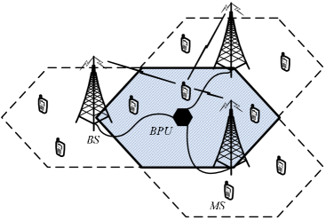
Consider a MIMO-MAC link with M𝑀M base stations and W𝑊W users operating over a Rayleigh channel where BS i𝑖i has nRisubscript𝑛subscript𝑅𝑖n_{R_{i}} receive antennas and user i𝑖i has nisubscript𝑛𝑖n_{i} antennas. The total number of receive antennas is denoted nR=i=1MnRisubscript𝑛𝑅superscriptsubscript𝑖1𝑀subscript𝑛subscript𝑅𝑖n_{R}=\sum_{i=1}^{M}n_{R_{i}} and the total number of transmit antennas is denoted N=i=1Wni𝑁superscriptsubscript𝑖1𝑊subscript𝑛𝑖N=\sum_{i=1}^{W}n_{i}. An example of such a system is shown in Fig. 1, where three BSs are linked by a backhaul processing unit (BPU) and communicate with multiple, mobile users. All channels are considered to be independent since the correlated channel scenario can be transformed into the independent case as shown in Sec. II-A. The system equation is given by

r=Hs+n,𝑟𝐻𝑠𝑛\displaystyle\mbox{\boldsymbol{$r$}}=\mbox{\boldsymbol{$Hs$}}+\mbox{\boldsymbol{$n$}}, (1)

where r𝑟r is the 𝒞nR×1superscript𝒞subscript𝑛𝑅1\mathcal{C}^{n_{R}\times 1} receive vector, s𝑠s is the combined 𝒞N×1superscript𝒞𝑁1\mathcal{C}^{N\times 1} transmitted vector from the W𝑊W users, n𝑛n is an additive white Gaussian noise vector, n𝒞𝒩(0,σ2I)similar-to𝑛𝒞𝒩0superscript𝜎2𝐼\mbox{\boldsymbol{$n$}}\sim\mathcal{CN}\left(\mbox{\boldsymbol{$0$}},\sigma^{2}\mbox{\boldsymbol{$I$}}\right), and H𝒞nR×N𝐻superscript𝒞subscript𝑛𝑅𝑁\mbox{\boldsymbol{$H$}}\in\mathcal{C}^{n_{R}\times N} is the composite channel matrix containing the W𝑊W channel matrices from the W𝑊W users. The ergodic sum capacity of the link depends on the availability of channel state information (CSI) at the transmitter side. In particular, if no CSI at the transmitter is assumed, the corresponding ergodic sum capacity is [3, pp. 57]

E{C}𝐸𝐶\displaystyle E\left\{C\right\} =E{log2|I+1σ2HHH|},absent𝐸subscript2𝐼1superscript𝜎2superscript𝐻𝐻𝐻\displaystyle=E\left\{\log_{2}\left|\mbox{\boldsymbol{$I$}}+\frac{1}{\sigma^{2}}\mbox{\boldsymbol{$HH$}}^{H}\right|\right\}, (2)

Refer to caption

Figure 1: A network MIMO system with a 3 sector cluster. To reduce the clutter, only paths from a single source are shown.

where E{|si|2}=1𝐸superscriptsubscript𝑠𝑖21E\left\{|s_{i}|^{2}\right\}=1, i=1,2,,N𝑖12𝑁i=1,2,\dots,N, is the power of each transmitted symbol. It is convenient to label each column of H𝐻H as hisubscript𝑖\mbox{\boldsymbol{$h$}}_{i}, i=1,2,,N𝑖12𝑁i=1,2,\dots,N, so that H=(h1,h2,,hN)𝐻subscript1subscript2subscript𝑁\mbox{\boldsymbol{$H$}}=\left(\mbox{\boldsymbol{$h$}}_{1},\mbox{\boldsymbol{$h$}}_{2},\dots,\mbox{\boldsymbol{$h$}}_{N}\right). The covariance matrix of hksubscript𝑘\mbox{\boldsymbol{$h$}}_{k} is defined by Pk=E{hkhkH}subscript𝑃𝑘𝐸subscript𝑘superscriptsubscript𝑘𝐻\mbox{\boldsymbol{$P$}}_{k}=E\left\{\mbox{\boldsymbol{$h$}}_{k}\mbox{\boldsymbol{$h$}}_{k}^{H}\right\} and Pk=diag(P1k,P2k,,PnRk)subscript𝑃𝑘diagsubscript𝑃1𝑘subscript𝑃2𝑘subscript𝑃subscript𝑛𝑅𝑘\mbox{\boldsymbol{$P$}}_{k}=\mbox{diag}\left(P_{1k},P_{2k},\dots,P_{n_{R}k}\right). Hence, the ikth𝑖superscript𝑘𝑡ik^{th} element of H𝐻H is 𝒞𝒩(0,Pik)𝒞𝒩0subscript𝑃𝑖𝑘\mathcal{CN}\left(0,P_{ik}\right). Using this notation, we can also express hksubscript𝑘\mbox{\boldsymbol{$h$}}_{k} as hk=Pk12uksubscript𝑘subscriptsuperscript𝑃12𝑘subscript𝑢𝑘\mbox{\boldsymbol{$h$}}_{k}=\mbox{\boldsymbol{$P$}}^{\frac{1}{2}}_{k}\mbox{\boldsymbol{$u$}}_{k}, where uk𝒞𝒩(0,I)similar-tosubscript𝑢𝑘𝒞𝒩0𝐼\mbox{\boldsymbol{$u$}}_{k}\sim\mathcal{CN}\left(\mbox{\boldsymbol{$0$}},\mbox{\boldsymbol{$I$}}\right). Note that, for convenience, all the power information is contained in the Pksubscript𝑃𝑘\mbox{\boldsymbol{$P$}}_{k} matrices so that there is no normalization of the channel and, in (2), the scaling factor in the capacity equation is simply 1/σ21superscript𝜎21/\sigma^{2}.

II-A Correlated Channels

Consider the general scenario where sources and/or BSs have multiple co-located antennas for transmission and reception. Here, spatial correlation may be present due to the co-located antennas [13, 14]. If a Kronecker correlation model is assumed, then the composite channel matrix is given by

H𝐻H =(Rr11200RrM12)(Hw,11Hw,1WHw,M1Hw,MW)(Rt11200RtW12),absentsuperscriptsubscript𝑅𝑟112missing-subexpression0missing-subexpressionmissing-subexpression0missing-subexpressionsuperscriptsubscript𝑅𝑟𝑀12subscript𝐻𝑤11subscript𝐻𝑤1𝑊subscript𝐻𝑤𝑀1subscript𝐻𝑤𝑀𝑊superscriptsubscript𝑅𝑡112missing-subexpression0missing-subexpressionmissing-subexpression0missing-subexpressionsuperscriptsubscript𝑅𝑡𝑊12\displaystyle=\!\left(\!\begin{smallmatrix}\mbox{\boldsymbol{$R$}}_{r1}^{\frac{1}{2}}&&\mbox{\boldsymbol{$0$}}\\ \ &\ddots&\\ \mbox{\boldsymbol{$0$}}&&\mbox{\boldsymbol{$R$}}_{rM}^{\frac{1}{2}}\\ \end{smallmatrix}\!\right)\!\!\left(\!\begin{smallmatrix}\mbox{\boldsymbol{$H$}}_{w,11}&\ldots&\mbox{\boldsymbol{$H$}}_{w,1W}\\ \vdots&\ddots&\vdots\\ \mbox{\boldsymbol{$H$}}_{w,M1}&\ldots&\mbox{\boldsymbol{$H$}}_{w,MW}\\ \end{smallmatrix}\!\right)\!\!\left(\!\begin{smallmatrix}\mbox{\boldsymbol{$R$}}_{t1}^{\frac{1}{2}}&&\mbox{\boldsymbol{$0$}}\\ &\ddots&\\ \mbox{\boldsymbol{$0$}}&&\mbox{\boldsymbol{$R$}}_{tW}^{\frac{1}{2}}\\ \end{smallmatrix}\!\right), (3)

where the 𝒞nRk×nisuperscript𝒞subscript𝑛subscript𝑅𝑘subscript𝑛𝑖\mathcal{C}^{n_{R_{k}}\times n_{i}} matrix, Hw,iksubscript𝐻𝑤𝑖𝑘\mbox{\boldsymbol{$H$}}_{w,ik}, has iid elements since all the channel powers from user k𝑘k to BS i𝑖i are the same. The matrix Rrisubscript𝑅𝑟𝑖\mbox{\boldsymbol{$R$}}_{ri} is the receive correlation matrix at BS i𝑖i and the matrix Rtksubscript𝑅𝑡𝑘\mbox{\boldsymbol{$R$}}_{tk} is the transmit correlation matrix at source k𝑘k as defined in [13]. Using the spectral decompositions, Rri=ΦriΛriΦriHsubscript𝑅𝑟𝑖subscriptΦ𝑟𝑖subscriptΛ𝑟𝑖superscriptsubscriptΦ𝑟𝑖𝐻\mbox{\boldsymbol{$R$}}_{ri}=\mbox{\boldsymbol{$\Phi$}}_{ri}\mbox{\boldsymbol{$\Lambda$}}_{ri}\mbox{\boldsymbol{$\Phi$}}_{ri}^{H} and Rtk=ΦtkΛtkΦtkHsubscript𝑅𝑡𝑘subscriptΦ𝑡𝑘subscriptΛ𝑡𝑘superscriptsubscriptΦ𝑡𝑘𝐻\mbox{\boldsymbol{$R$}}_{tk}=\mbox{\boldsymbol{$\Phi$}}_{tk}\mbox{\boldsymbol{$\Lambda$}}_{tk}\mbox{\boldsymbol{$\Phi$}}_{tk}^{H} and substituting (3) into (2) it is easily shown that the capacity with the channel in (3) is statistically identical to the capacity with channel

H𝐻H =(Λr11200ΛrM12)(Hw,11Hw,1WHw,M1Hw,MW)(Λt11200ΛtW12).absentsuperscriptsubscriptΛ𝑟112missing-subexpression0missing-subexpressionmissing-subexpression0missing-subexpressionsuperscriptsubscriptΛ𝑟𝑀12subscript𝐻𝑤11subscript𝐻𝑤1𝑊subscript𝐻𝑤𝑀1subscript𝐻𝑤𝑀𝑊superscriptsubscriptΛ𝑡112missing-subexpression0missing-subexpressionmissing-subexpression0missing-subexpressionsuperscriptsubscriptΛ𝑡𝑊12\displaystyle=\!\left(\!\begin{smallmatrix}\mbox{\boldsymbol{$\Lambda$}}_{r1}^{\frac{1}{2}}&&\mbox{\boldsymbol{$0$}}\\ \ &\ddots&\\ \mbox{\boldsymbol{$0$}}&&\mbox{\boldsymbol{$\Lambda$}}_{rM}^{\frac{1}{2}}\\ \end{smallmatrix}\!\right)\!\!\left(\!\begin{smallmatrix}\mbox{\boldsymbol{$H$}}_{w,11}&\ldots&\mbox{\boldsymbol{$H$}}_{w,1W}\\ \vdots&\ddots&\vdots\\ \mbox{\boldsymbol{$H$}}_{w,M1}&\ldots&\mbox{\boldsymbol{$H$}}_{w,MW}\\ \end{smallmatrix}\!\right)\!\!\left(\!\begin{smallmatrix}\mbox{\boldsymbol{$\Lambda$}}_{t1}^{\frac{1}{2}}&&\mbox{\boldsymbol{$0$}}\\ &\ddots&\\ \mbox{\boldsymbol{$0$}}&&\mbox{\boldsymbol{$\Lambda$}}_{tW}^{\frac{1}{2}}\\ \end{smallmatrix}\!\right). (4)

Denoting (4) by H=Λr12HwΛt12𝐻superscriptsubscriptΛ𝑟12subscript𝐻𝑤superscriptsubscriptΛ𝑡12\mbox{\boldsymbol{$H$}}=\mbox{\boldsymbol{$\Lambda$}}_{r}^{\frac{1}{2}}\mbox{\boldsymbol{$H$}}_{w}\mbox{\boldsymbol{$\Lambda$}}_{t}^{\frac{1}{2}}, we see that correlation is equivalent to a scaling of the channel by the relevant eigenvalues in ΛrsubscriptΛ𝑟\mbox{\boldsymbol{$\Lambda$}}_{r} and ΛtsubscriptΛ𝑡\mbox{\boldsymbol{$\Lambda$}}_{t}. In particular, the (u,v)thsuperscript𝑢𝑣𝑡\left(u,v\right)^{th} element of H𝐻H has power Λr,uuΛt,vvPuvsubscriptΛ𝑟𝑢𝑢subscriptΛ𝑡𝑣𝑣subscript𝑃𝑢𝑣\mbox{\boldsymbol{$\Lambda$}}_{r,uu}\mbox{\boldsymbol{$\Lambda$}}_{t,vv}P_{uv}, where Puvsubscript𝑃𝑢𝑣P_{uv} is the single link power from transmit antenna v𝑣v to receive antenna u𝑢u. Hence, correlation can be handled by the same methodology developed in Secs. IV-VI, with suitably scaled power values 111Arbitrary fixed transmit power control techniques can also be handled in the same way as for the correlated scenario..

III Preliminaries

In this section we derive some useful results which will be used extensively throughout the paper.

Lemma 1.

Let X𝑋X be an n×n𝑛𝑛n\times n complex random matrix with,

A𝐴A =E{XX}(E{|X11|2}E{|X12|2}E{|X21|2}E{|X22|2}E{|Xn1|2}E{|Xn2|2}),absent𝐸𝑋𝑋𝐸superscriptsubscript𝑋112𝐸superscriptsubscript𝑋122𝐸superscriptsubscript𝑋212𝐸superscriptsubscript𝑋222𝐸superscriptsubscript𝑋𝑛12𝐸superscriptsubscript𝑋𝑛22\displaystyle=\!E\left\{\mbox{\boldsymbol{$X$}}\circ\mbox{\boldsymbol{$X$}}\right\}\triangleq\!\left(\!\begin{array}[]{ccc}\vspace{1mm}E\left\{|X_{11}|^{2}\right\}&E\left\{|X_{12}|^{2}\right\}&\ldots\\ \vspace{1mm}E\left\{|X_{21}|^{2}\right\}&E\left\{|X_{22}|^{2}\right\}&\ldots\\ \vspace{1mm}\ldots&\ldots&\ldots\\ E\left\{|X_{n1}|^{2}\right\}&E\left\{|X_{n2}|^{2}\right\}&\ldots\\ \end{array}\!\right)\!, (9)

where \circ represents the Hadamard product. With this notation, the following identity holds.

E{|XHX|}𝐸superscript𝑋𝐻𝑋\displaystyle E\left\{\left|\mbox{\boldsymbol{$X$}}^{H}\mbox{\boldsymbol{$X$}}\right|\right\} =perm(A),absentperm𝐴\displaystyle=\mbox{perm}\left(\mbox{\boldsymbol{$A$}}\right), (10)

where perm(.)perm(.) is the permanent of a square matrix defined in [15].

Proof.

From the definition of the determinant of a generic matrix, X={Xi,k}i,k=1n𝑋subscriptsubscript𝑋𝑖𝑘𝑖𝑘1𝑛\mbox{\boldsymbol{$X$}}=\left\{X_{i,k}\right\}_{i,k=1\dots n}, we have

E{|XHX|}=E{[σsgn(σ)i=1nX¯σi,i]×[μsgn(μ)i=1nXμi,i]},𝐸superscript𝑋𝐻𝑋𝐸delimited-[]subscript𝜎sgn𝜎superscriptsubscriptproduct𝑖1𝑛subscript¯𝑋subscript𝜎𝑖𝑖delimited-[]subscript𝜇sgn𝜇superscriptsubscriptproduct𝑖1𝑛subscript𝑋subscript𝜇𝑖𝑖\displaystyle\begin{split}E\left\{\left|\mbox{\boldsymbol{$X$}}^{H}\mbox{\boldsymbol{$X$}}\right|\right\}=E&\left\{\left[\sum_{\sigma}\mbox{sgn}(\sigma)\prod_{i=1}^{n}\bar{X}_{\sigma_{i},i}\right]\right.\times\left.\left[\sum_{\mu}\mbox{sgn}(\mu)\prod_{i=1}^{n}X_{\mu_{i},i}\right]\right\},\end{split} (11)

where σ=(σ1,σ2,,σn)𝜎subscript𝜎1subscript𝜎2subscript𝜎𝑛\sigma=\left(\sigma_{1},\sigma_{2},\dots,\sigma_{n}\right) is a permutation of the integers 1,,n1𝑛1,\dots,n, the sum is over all permutations, and sgn(σ)sgn𝜎\mbox{sgn}(\sigma) denotes the sign of the permutation. The permutation, μ𝜇\mu, in the second summation of (11) is defined similarly. Since all the elements of X𝑋X are independent, the only terms giving non-zero value expectations are i=1nX¯ai,ii=1nXbi,isuperscriptsubscriptproduct𝑖1𝑛subscript¯𝑋subscript𝑎𝑖𝑖superscriptsubscriptproduct𝑖1𝑛subscript𝑋subscript𝑏𝑖𝑖\prod_{i=1}^{n}\bar{X}_{a_{i},i}\prod_{i=1}^{n}X_{b_{i},i}, where permutation a=b𝑎𝑏a=b. Hence, using the permanent definition in [15] we have

E{|XHX|}=σi=1nAσi,i=perm(A).𝐸superscript𝑋𝐻𝑋subscript𝜎superscriptsubscriptproduct𝑖1𝑛subscript𝐴subscript𝜎𝑖𝑖perm𝐴\displaystyle\begin{split}E\left\{\left|\mbox{\boldsymbol{$X$}}^{H}\mbox{\boldsymbol{$X$}}\right|\right\}&=\sum_{\sigma}\prod_{i=1}^{n}A_{\sigma_{i},i}=\mbox{perm}\left(\mbox{\boldsymbol{$A$}}\right).\end{split} (12)

Corollary 1.

Let X𝑋X be an m×n𝑚𝑛m\times n random matrix with, E{XX}=A𝐸𝑋𝑋𝐴E\left\{\mbox{\boldsymbol{$X$}}\circ\mbox{\boldsymbol{$X$}}\right\}=\mbox{\boldsymbol{$A$}}, where A𝐴A is an m×n𝑚𝑛m\times n deterministic matrix and m>n𝑚𝑛m>n. Then, the following identity holds.

E{|XHX|}=Perm(A),𝐸superscript𝑋𝐻𝑋Perm𝐴\displaystyle\begin{split}E\left\{\left|\mbox{\boldsymbol{$X$}}^{H}\mbox{\boldsymbol{$X$}}\right|\right\}=\mbox{Perm}\left(\mbox{\boldsymbol{$A$}}\right),\end{split} (13)

where Perm(A)Perm𝐴\mbox{Perm}\left(\mbox{\boldsymbol{$A$}}\right) is the permanent of the rectangular matrix A𝐴A as defined in [15].

Proof.

Using the Cauchy-Binet formula for the determinant of the product of two rectangular matrices, we can expand |XHX|superscript𝑋𝐻𝑋\left|\mbox{\boldsymbol{$X$}}^{H}\mbox{\boldsymbol{$X$}}\right| as a sum of products of two square matrices. Each product of square matrices can be evaluated using Lemma 1. The resulting expression is seen to be the permanent of the rectangular matrix, A𝐴A, which completes the proof. ∎

Corollary 2.

Let X𝑋X be an m×n𝑚𝑛m\times n random matrix with, E{XX}=A𝐸𝑋𝑋𝐴E\left\{\mbox{\boldsymbol{$X$}}\circ\mbox{\boldsymbol{$X$}}\right\}=\mbox{\boldsymbol{$A$}}, where A𝐴A is an m×n𝑚𝑛m\times n deterministic matrix and m>n𝑚𝑛m>n. If the m×m𝑚𝑚m\times m deterministic matrix ΣΣ\Sigma is diagonal, then the following identity holds.

E{|XHΣX|}=Perm(ΣA).𝐸superscript𝑋𝐻ΣXPermΣA\displaystyle\begin{split}E\left\{\left|\mbox{\boldsymbol{$X$}}^{H}\mbox{\boldsymbol{$\Sigma$}}\mbox{\boldsymbol{$X$}}\right|\right\}=\mbox{Perm}\left(\mbox{\boldsymbol{$\Sigma$}}\mbox{\boldsymbol{$A$}}\right).\end{split} (14)
Proof.

The result follows directly from Lemma 1, and the fact that Σ12Σ12=ΣsuperscriptΣ12superscriptΣ12Σ\mbox{\boldsymbol{$\Sigma$}}^{\frac{1}{2}}\circ\mbox{\boldsymbol{$\Sigma$}}^{\frac{1}{2}}=\mbox{\boldsymbol{$\Sigma$}} for any diagonal matrix. ∎

Next, we give a definition for the elementary symmetric function (esf) of degree k𝑘k in n𝑛n variables, X1,X2,,Xnsubscript𝑋1subscript𝑋2subscript𝑋𝑛X_{1},X_{2},\dots,X_{n} [16]. Let ek(X1,X2,,Xn)subscript𝑒𝑘subscript𝑋1subscript𝑋2subscript𝑋𝑛e_{k}\left(X_{1},X_{2},\dots,X_{n}\right) be the kthsuperscript𝑘𝑡k^{th} degree esf, then

ek(X1,X2,,Xn)subscript𝑒𝑘subscript𝑋1subscript𝑋2subscript𝑋𝑛\displaystyle e_{k}\left(X_{1},X_{2},\dots,X_{n}\right) =1l1<l2<<lknXl1Xlk.absentsubscript1subscript𝑙1subscript𝑙2subscript𝑙𝑘𝑛subscript𝑋subscript𝑙1subscript𝑋subscript𝑙𝑘\displaystyle=\sum_{1\leq l_{1}<l_{2}<\dots<l_{k}\leq n}X_{l_{1}}\dots X_{l_{k}}. (15)

It is apparent from (15) that e0(X1,X2,,Xn)=1subscript𝑒0subscript𝑋1subscript𝑋2subscript𝑋𝑛1e_{0}\left(X_{1},X_{2},\dots,X_{n}\right)=1 and en(X1,X2,,Xn)=X1X2Xnsubscript𝑒𝑛subscript𝑋1subscript𝑋2subscript𝑋𝑛subscript𝑋1subscript𝑋2subscript𝑋𝑛e_{n}\left(X_{1},X_{2},\dots,X_{n}\right)=X_{1}X_{2}\dots X_{n}. In general, the esf of degree k𝑘k in n𝑛n variables, for any kn𝑘𝑛k\leq n, is formed by adding together all distinct products of k𝑘k distinct variables.

Lemma 2.

[16] let X𝑋X be an n×n𝑛𝑛n\times n complex symmetric positive definite matrix with eigenvalues λ1,,λnsubscript𝜆1subscript𝜆𝑛\lambda_{1},\dots,\lambda_{n}. Then, the following identity holds.

ek(λ1,λ2,,λn)subscript𝑒𝑘subscript𝜆1subscript𝜆2subscript𝜆𝑛\displaystyle e_{k}\left(\lambda_{1},\lambda_{2},\dots,\lambda_{n}\right) =Trk(X),absentsubscriptTr𝑘𝑋\displaystyle=\textup{\mbox{Tr}}_{k}\left(\mbox{\boldsymbol{$X$}}\right), (16)

where

Trk(X)={σ|Xσk,n|1kn1k=00k>n,subscriptTr𝑘𝑋casessubscript𝜎subscript𝑋subscript𝜎𝑘𝑛1𝑘𝑛1𝑘00𝑘𝑛\displaystyle\textup{\mbox{Tr}}_{k}\left(\mbox{\boldsymbol{$X$}}\right)=\begin{cases}\sum_{\sigma}\left|\mbox{\boldsymbol{$X$}}_{\sigma_{k,n}}\right|&\quad 1\leq k\leq n\\ 1&\quad k=0\\ 0&\quad k>n,\end{cases} (17)

where σk,nsubscript𝜎𝑘𝑛\sigma_{k,n} is an ordered subset of {n}={1,,n}𝑛1𝑛\left\{n\right\}=\left\{1,\dots,n\right\} of length k𝑘k and the summation is over all such subsets. Xσk,nsubscript𝑋subscript𝜎𝑘𝑛\left.\mbox{\boldsymbol{$X$}}\right._{\sigma_{k,n}} denotes the principal submatrix of X𝑋X formed by taking only the rows and columns indexed by σk,nsubscript𝜎𝑘𝑛\sigma_{k,n}.
In general, Xσ,nμ,nsuperscriptsubscript𝑋subscript𝜎𝑛subscript𝜇𝑛\left.\mbox{\boldsymbol{$X$}}\right._{\sigma_{\ell,n}}^{\mu_{\ell,n}} denotes the submatrix of X𝑋X formed by taking only the rows and columns indexed by σ,nsubscript𝜎𝑛\sigma_{\ell,n} and μ,nsubscript𝜇𝑛\mu_{\ell,n} respectively, where σ,nsubscript𝜎𝑛\sigma_{\ell,n} and μ,nsubscript𝜇𝑛\mu_{\ell,n} are length \ell subsets of {1,2,,n}12𝑛\{1,2,\dots,n\}. If either σ,nsubscript𝜎𝑛\sigma_{\ell,n} or μ,nsubscript𝜇𝑛\mu_{\ell,n} contains the complete set (i.e., σ,n={1,2,,n}subscript𝜎𝑛12𝑛\sigma_{\ell,n}=\{1,2,\dots,n\} or μ,n={1,2,,n}subscript𝜇𝑛12𝑛\mu_{\ell,n}=\{1,2,\dots,n\}), the corresponding subscript/superscript may be dropped. When σ,n=μ,nsubscript𝜎𝑛subscript𝜇𝑛\sigma_{\ell,n}=\mu_{\ell,n}, only one subscript/superscript may be shown for brevity.
Next, we present three axiomatic identities for permanents which are required in Sec. V.

  • Axiom 1: Let A𝐴A be an arbitrary m×n𝑚𝑛m\times n matrix, then

    σPerm((A)μ0,n)subscript𝜎Permsuperscript𝐴subscript𝜇0𝑛\displaystyle\sum_{\sigma}\mbox{Perm}\left(\left(\mbox{\boldsymbol{$A$}}\right)^{\mu_{0,n}}\right) =σPerm((A)σ0,m)=1.absentsubscript𝜎Permsubscript𝐴subscript𝜎0𝑚1\displaystyle=\sum_{\sigma}\mbox{Perm}\left(\left(\mbox{\boldsymbol{$A$}}\right)_{\sigma_{0,m}}\right)=1. (18)
  • Axiom 2: Let A𝐴A be an arbitrary m×n𝑚𝑛m\times n matrix, then

    σPerm((A)σk,m)subscript𝜎Permsubscript𝐴subscript𝜎𝑘𝑚\displaystyle\sum_{\sigma}\mbox{Perm}\left(\left(\mbox{\boldsymbol{$A$}}\right)_{\sigma_{k,m}}\right) =σPerm((A)σk,n).absentsubscript𝜎Permsuperscript𝐴subscript𝜎𝑘𝑛\displaystyle=\sum_{\sigma}\mbox{Perm}\left(\left(\mbox{\boldsymbol{$A$}}\right)^{\sigma_{k,n}}\right). (19)
  • Axiom 3: For an empty matrix, A𝐴A,

    Perm(A)Perm𝐴\displaystyle\mbox{Perm}\left(\mbox{\boldsymbol{$A$}}\right) =1.absent1\displaystyle=1. (20)

IV Exact Small System Analysis

In this section, we derive the exact ergodic sum capacity in (2) for the N=2𝑁2N=2 case. This corresponds to two single antenna users or a single user with two distributed antennas. Here, the channel matrix becomes H=(h1,h2)𝐻subscript1subscript2\mbox{\boldsymbol{$H$}}=\left(\mbox{\boldsymbol{$h$}}_{1},\mbox{\boldsymbol{$h$}}_{2}\right) and it is straightforward to write (2) as

E{C}ln2𝐸𝐶2\displaystyle E\left\{C\right\}\ln 2 =E{ln|I+1σ2h1h1H|}absent𝐸𝐼1superscript𝜎2subscript1superscriptsubscript1𝐻\displaystyle=E\left\{\ln\left|\mbox{\boldsymbol{$I$}}+\frac{1}{\sigma^{2}}\mbox{\boldsymbol{$h$}}_{1}\mbox{\boldsymbol{$h$}}_{1}^{H}\right|\right\}
+E{ln|I+1σ2(I+1σ2h1h1H)1h2h2H|}𝐸𝐼1superscript𝜎2superscript𝐼1superscript𝜎2subscript1superscriptsubscript1𝐻1subscript2superscriptsubscript2𝐻\displaystyle+\!E\left\{\ln\left|\mbox{\boldsymbol{$I$}}\!+\!\frac{1}{\sigma^{2}}\left(\mbox{\boldsymbol{$I$}}\!+\!\frac{1}{\sigma^{2}}\mbox{\boldsymbol{$h$}}_{1}\mbox{\boldsymbol{$h$}}_{1}^{H}\right)^{-1}\!\!\!\mbox{\boldsymbol{$h$}}_{2}\mbox{\boldsymbol{$h$}}_{2}^{H}\right|\right\}
C1+C2.absentsubscript𝐶1subscript𝐶2\displaystyle\triangleq C_{1}+C_{2}. (21)

Both C1subscript𝐶1C_{1} and C2subscript𝐶2C_{2} can be expressed as scalars [17], [18, pp. 48], so the capacity analysis simply requires

C1subscript𝐶1\displaystyle C_{1} =E{ln(1+1σ2h1Hh1)},absent𝐸11superscript𝜎2superscriptsubscript1𝐻subscript1\displaystyle=E\left\{\ln\left(1+\frac{1}{\sigma^{2}}\mbox{\boldsymbol{$h$}}_{1}^{H}\mbox{\boldsymbol{$h$}}_{1}\right)\right\}, (22)
C2subscript𝐶2\displaystyle C_{2} =E{ln(1+1σ2h2H(I+1σ2h1h1H)1h2)}.absent𝐸11superscript𝜎2superscriptsubscript2𝐻superscript𝐼1superscript𝜎2subscript1superscriptsubscript1𝐻1subscript2\displaystyle=E\left\{\ln\left(1\!+\!\frac{1}{\sigma^{2}}\mbox{\boldsymbol{$h$}}_{2}^{H}\left(\mbox{\boldsymbol{$I$}}\!+\!\frac{1}{\sigma^{2}}\mbox{\boldsymbol{$h$}}_{1}\mbox{\boldsymbol{$h$}}_{1}^{H}\right)^{-1}\!\!\!\mbox{\boldsymbol{$h$}}_{2}\right)\right\}. (23)

In order to facilitate our analysis, it is useful to avoid the logarithm representations in (22) and (23). We exchange logarithms for exponentials as follows. First, we note the identity,

1a1𝑎\displaystyle\frac{1}{a} =0eat𝑑t,fora>0.formulae-sequenceabsentsuperscriptsubscript0superscript𝑒𝑎𝑡differential-d𝑡for𝑎0\displaystyle=\int_{0}^{\infty}e^{-at}dt,\quad\mbox{for}\quad a>0. (24)

Now equation (24) can be used to find lna𝑎\ln a as below:

lnaa𝑎𝑎\displaystyle\frac{\partial\ln a}{\partial a} =0eat𝑑t,absentsuperscriptsubscript0superscript𝑒𝑎𝑡differential-d𝑡\displaystyle=\int_{0}^{\infty}e^{-at}dt, (25)
0lnadlnasuperscriptsubscript0𝑎𝑑𝑎\displaystyle\int_{0}^{\ln a}d\ln a =1a0eat𝑑t𝑑a,absentsuperscriptsubscript1𝑎superscriptsubscript0superscript𝑒𝑎𝑡differential-d𝑡differential-d𝑎\displaystyle=\int_{1}^{a}\int_{0}^{\infty}e^{-at}dtda, (26)
lna𝑎\displaystyle\ln a =0eteatt𝑑t.absentsuperscriptsubscript0superscript𝑒𝑡superscript𝑒𝑎𝑡𝑡differential-d𝑡\displaystyle=\int_{0}^{\infty}\frac{e^{-t}-e^{-at}}{t}dt. (27)

This manipulation is useful because there are many results which can be applied to exponentials of quadratic forms, whereas few results exist for logarithms. As an example, using (27) in (22) gives

C1subscript𝐶1\displaystyle C_{1} =E{0ete(1+1σ2h1Hh1)tt𝑑t}.absent𝐸superscriptsubscript0superscript𝑒𝑡superscript𝑒11superscript𝜎2superscriptsubscript1𝐻subscript1𝑡𝑡differential-d𝑡\displaystyle=E\left\{\int_{0}^{\infty}\frac{e^{-t}-e^{-\left(1+\frac{1}{\sigma^{2}}\mbox{\boldsymbol{$h$}}_{1}^{H}\mbox{\boldsymbol{$h$}}_{1}\right)t}}{t}dt\right\}. (28)

Note that a=1+1σ2h1Hh1𝑎11superscript𝜎2superscriptsubscript1𝐻subscript1a=1+\frac{1}{\sigma^{2}}\mbox{\boldsymbol{$h$}}_{1}^{H}\mbox{\boldsymbol{$h$}}_{1} has been used in (27). Sice a1𝑎1a\geq 1, it follows that the integrand in (28) is non-negative. Also, the expected value, C1subscript𝐶1C_{1}, is clearly finite and so, by Fubini’s theorem, the order of expectation and integration in (28) may be interchanged. Using the Gaussian integral identity [9], the expectation in (28) can be computed to give

C1subscript𝐶1\displaystyle C_{1} =0ettett|Σ1|dt,absentsuperscriptsubscript0superscript𝑒𝑡𝑡superscript𝑒𝑡𝑡subscriptΣ1𝑑𝑡\displaystyle=\int_{0}^{\infty}\frac{e^{-t}}{t}-\frac{e^{-t}}{t\left|\mbox{\boldsymbol{$\Sigma$}}_{1}\right|}dt, (29)

where Σ1=I+tσ2P1subscriptΣ1𝐼𝑡superscript𝜎2subscript𝑃1\mbox{\boldsymbol{$\Sigma$}}_{1}=\mbox{\boldsymbol{$I$}}+\frac{t}{\sigma^{2}}\mbox{\boldsymbol{$P$}}_{1}. Hence, the log-exponential conversion in (27) leads to a manageable integral for C1subscript𝐶1C_{1}. Using the same approach and applying (27) in (23) gives

C2subscript𝐶2\displaystyle C_{2} =E{0ettettσ2h2H(I+1σ2h1h1H)1h2tdt}.absent𝐸superscriptsubscript0superscript𝑒𝑡𝑡superscript𝑒𝑡𝑡superscript𝜎2superscriptsubscript2𝐻superscript𝐼1superscript𝜎2subscript1superscriptsubscript1𝐻1subscript2𝑡𝑑𝑡\displaystyle=E\left\{\int_{0}^{\infty}\frac{e^{-t}}{t}-\frac{e^{-t-\frac{t}{\sigma^{2}}\mbox{\boldsymbol{$h$}}_{2}^{H}\left(\mbox{\boldsymbol{$I$}}+\frac{1}{\sigma^{2}}\mbox{\boldsymbol{$h$}}_{1}\mbox{\boldsymbol{$h$}}_{1}^{H}\right)^{-1}\mbox{\boldsymbol{$h$}}_{2}}}{t}dt\right\}. (30)

The expectation in (30) has to be calculated in two stages. First, the expectation over h2subscript2\mbox{\boldsymbol{$h$}}_{2} can be solved using the Gaussian integral identity [9] and, with some simplifications, we arrive at

C2subscript𝐶2\displaystyle C_{2}\! =0ettEh1{et(σ2+h1Hh1)t|Σ2|(σ2+h1HΣ21h1)}dt,absentsuperscriptsubscript0superscript𝑒𝑡𝑡subscript𝐸subscript1superscript𝑒𝑡superscript𝜎2superscriptsubscript1𝐻subscript1𝑡subscriptΣ2superscript𝜎2superscriptsubscript1𝐻superscriptsubscriptΣ21subscript1𝑑𝑡\displaystyle=\!\int_{0}^{\infty}\!\!\frac{e^{-t}}{t}-E_{\mbox{\boldsymbol{$h$}}_{1}}\!\left\{\frac{e^{-t}\left(\sigma^{2}+\mbox{\boldsymbol{$h$}}_{1}^{H}\mbox{\boldsymbol{$h$}}_{1}\right)}{t\left|\mbox{\boldsymbol{$\Sigma$}}_{2}\right|\left(\sigma^{2}+\mbox{\boldsymbol{$h$}}_{1}^{H}\mbox{\boldsymbol{$\Sigma$}}_{2}^{-1}\mbox{\boldsymbol{$h$}}_{1}\right)}\right\}dt, (31)

where Σ2=I+tσ2P2subscriptΣ2𝐼𝑡superscript𝜎2subscript𝑃2\mbox{\boldsymbol{$\Sigma$}}_{2}=\mbox{\boldsymbol{$I$}}+\frac{t}{\sigma^{2}}\mbox{\boldsymbol{$P$}}_{2}. Interchange of the expectation and integral in (31) follows from the same arguments used for C1subscript𝐶1C_{1}. Equation (31) can be further simplified to give

C2=subscript𝐶2absent\displaystyle C_{2}= 0ettett|Σ2|dtEh1{1σ20eth1HP2Σ21h1t|Σ2|(σ2+h1HΣ21h1)𝑑t}.superscriptsubscript0superscript𝑒𝑡𝑡superscript𝑒𝑡𝑡subscriptΣ2𝑑𝑡subscript𝐸subscript11superscript𝜎2superscriptsubscript0superscript𝑒𝑡superscriptsubscript1𝐻subscript𝑃2superscriptsubscriptΣ21subscript1𝑡subscriptΣ2superscript𝜎2superscriptsubscript1𝐻superscriptsubscriptΣ21subscript1differential-d𝑡\displaystyle\int_{0}^{\infty}\frac{e^{-t}}{t}-\frac{e^{-t}}{t\left|\mbox{\boldsymbol{$\Sigma$}}_{2}\right|}dt-E_{\mbox{\boldsymbol{$h$}}_{1}}\!\left\{\!\frac{1}{\sigma^{2}}\int_{0}^{\infty}\frac{e^{-t}\mbox{\boldsymbol{$h$}}_{1}^{H}\mbox{\boldsymbol{$P$}}_{2}\mbox{\boldsymbol{$\Sigma$}}_{2}^{-1}\mbox{\boldsymbol{$h$}}_{1}}{t\left|\mbox{\boldsymbol{$\Sigma$}}_{2}\right|\left(\sigma^{2}+\mbox{\boldsymbol{$h$}}_{1}^{H}\mbox{\boldsymbol{$\Sigma$}}_{2}^{-1}\mbox{\boldsymbol{$h$}}_{1}\right)}dt\right\}. (32)

Defining the third term in (32) as Ibsubscript𝐼𝑏I_{b}, the ergodic sum capacity, E(C)=C1+C2𝐸𝐶subscript𝐶1subscript𝐶2E\left(C\right)=C_{1}+C_{2}, becomes

E{C}𝐸𝐶\displaystyle E\left\{C\right\} =1ln2{k=12IakIb},absent12superscriptsubscript𝑘12subscript𝐼subscript𝑎𝑘subscript𝐼𝑏\displaystyle=\frac{1}{\ln 2}\left\{\sum_{k=1}^{2}I_{a_{k}}-I_{b}\right\}, (33)

where

Iaksubscript𝐼subscript𝑎𝑘\displaystyle I_{a_{k}} =0(ettett|Σk|)𝑑t.absentsuperscriptsubscript0superscript𝑒𝑡𝑡superscript𝑒𝑡𝑡subscriptΣ𝑘differential-d𝑡\displaystyle=\int_{0}^{\infty}\left(\frac{e^{-t}}{t}-\frac{e^{-t}}{t\left|\mbox{\boldsymbol{$\Sigma$}}_{k}\right|}\right)dt. (34)

Substituting for ΣksubscriptΣ𝑘\mbox{\boldsymbol{$\Sigma$}}_{k} in (34) and expanding (t|Σk|)1superscript𝑡subscriptΣ𝑘1\left(t\left|\mbox{\boldsymbol{$\Sigma$}}_{k}\right|\right)^{-1} gives

Iaksubscript𝐼subscript𝑎𝑘\displaystyle I_{a_{k}} =i=1nRηik0ett+σ2Pik𝑑t,absentsuperscriptsubscript𝑖1subscript𝑛𝑅subscript𝜂𝑖𝑘superscriptsubscript0superscript𝑒𝑡𝑡superscript𝜎2subscript𝑃𝑖𝑘differential-d𝑡\displaystyle=\sum_{i=1}^{n_{R}}\eta_{ik}\int_{0}^{\infty}\frac{e^{-t}}{t+\frac{\sigma^{2}}{P_{ik}}}dt, (35)

where

ηiksubscript𝜂𝑖𝑘\displaystyle\eta_{ik} =PiknR1linR(PikPlk).absentsuperscriptsubscript𝑃𝑖𝑘subscript𝑛𝑅1superscriptsubscriptproduct𝑙𝑖subscript𝑛𝑅subscript𝑃𝑖𝑘subscript𝑃𝑙𝑘\displaystyle=\frac{P_{ik}^{n_{R}-1}}{\prod_{l\neq i}^{n_{R}}\left(P_{ik}-P_{lk}\right)}. (36)

Note that the first et/tsuperscript𝑒𝑡𝑡e^{-t}/t term in (34) cancels out with one of the terms in the partial fraction expansion leaving only the linear terms shown in the denominator of (35). The integrals in (35) can be solved in closed form [19] to give

Iaksubscript𝐼subscript𝑎𝑘\displaystyle I_{a_{k}} =i=1nRηikeσ2PikE1(σ2Pik).absentsuperscriptsubscript𝑖1subscript𝑛𝑅subscript𝜂𝑖𝑘superscript𝑒superscript𝜎2subscript𝑃𝑖𝑘subscript𝐸1superscript𝜎2subscript𝑃𝑖𝑘\displaystyle=\sum_{i=1}^{n_{R}}\eta_{ik}e^{\frac{\sigma^{2}}{P_{ik}}}E_{1}\left(\frac{\sigma^{2}}{P_{ik}}\right). (37)

In order to compute Ibsubscript𝐼𝑏I_{b} we use [9, Lemma 1] to give

Ib=00et|Σ2|E{eθ1z1θ2z2}θ1|θ1=0dθ2dt,subscript𝐼𝑏evaluated-atsuperscriptsubscript0superscriptsubscript0superscript𝑒𝑡subscriptΣ2𝐸superscript𝑒subscript𝜃1subscript𝑧1subscript𝜃2subscript𝑧2subscript𝜃1subscript𝜃10𝑑subscript𝜃2𝑑𝑡I_{b}=-\int_{0}^{\infty}\int_{0}^{\infty}\frac{e^{-t}}{\left|\mbox{\boldsymbol{$\Sigma$}}_{2}\right|}\left.\frac{\partial E\left\{e^{-\theta_{1}z_{1}-\theta_{2}z_{2}}\right\}}{\partial\theta_{1}}\right|_{\theta_{1}=0}d\theta_{2}dt, (38)

where z1=h1HP2Σ21h1subscript𝑧1superscriptsubscript1𝐻subscript𝑃2superscriptsubscriptΣ21subscript1z_{1}=\mbox{\boldsymbol{$h$}}_{1}^{H}\mbox{\boldsymbol{$P$}}_{2}\mbox{\boldsymbol{$\Sigma$}}_{2}^{-1}\mbox{\boldsymbol{$h$}}_{1} and z2=σ2+h1HΣ21h1subscript𝑧2superscript𝜎2superscriptsubscript1𝐻superscriptsubscriptΣ21subscript1z_{2}=\sigma^{2}+\mbox{\boldsymbol{$h$}}_{1}^{H}\mbox{\boldsymbol{$\Sigma$}}_{2}^{-1}\mbox{\boldsymbol{$h$}}_{1}. The expectation in (38) can be solved as in [9], and with some manipulations we arrive at

Ib=00θ1[eσ2tσ2θ2|I+tP2+θ1P1P2+θ2P1|]θ1=0𝑑θ2𝑑t.subscript𝐼𝑏superscriptsubscript0superscriptsubscript0subscript𝜃1subscriptdelimited-[]superscript𝑒superscript𝜎2𝑡superscript𝜎2subscript𝜃2𝐼𝑡subscript𝑃2subscript𝜃1subscript𝑃1subscript𝑃2subscript𝜃2subscript𝑃1subscript𝜃10differential-dsubscript𝜃2differential-d𝑡I_{b}=-\!\!\int_{0}^{\infty}\!\!\!\!\int_{0}^{\infty}\!\!\frac{\partial}{\partial\theta_{1}}\!\!\left[\frac{e^{-\sigma^{2}t-\sigma^{2}\theta_{2}}}{\left|\mbox{\boldsymbol{$I$}}+t\mbox{\boldsymbol{$P$}}_{2}+\theta_{1}\mbox{\boldsymbol{$P$}}_{1}\mbox{\boldsymbol{$P$}}_{2}+\theta_{2}\mbox{\boldsymbol{$P$}}_{1}\right|}\right]_{\theta_{1}=0}\!\!\!d\theta_{2}dt. (39)

In Appendix A, Ibsubscript𝐼𝑏I_{b} in (39) is calculated in closed form and the final result is given by

Ibsubscript𝐼𝑏\displaystyle I_{b} =1|P1P2|{i=1nRkinRli,knRξikl(M~biklN~bikl)Ji},absent1subscript𝑃1subscript𝑃2superscriptsubscript𝑖1subscript𝑛𝑅superscriptsubscript𝑘𝑖subscript𝑛𝑅superscriptsubscript𝑙𝑖𝑘subscript𝑛𝑅subscript𝜉𝑖𝑘𝑙subscript~𝑀subscript𝑏𝑖𝑘𝑙subscript~𝑁subscript𝑏𝑖𝑘𝑙subscript𝐽𝑖\displaystyle=-\frac{1}{\left|\mbox{\boldsymbol{$P$}}_{1}\mbox{\boldsymbol{$P$}}_{2}\right|}\left\{\sum_{i=1}^{n_{R}}\sum_{k\neq i}^{n_{R}}\sum_{l\neq i,k}^{n_{R}}\frac{\xi_{ikl}\left(\tilde{M}_{b_{ikl}}-\tilde{N}_{b_{ikl}}\right)}{J_{i}}\right\}, (40)

where M~biklsubscript~𝑀subscript𝑏𝑖𝑘𝑙\tilde{M}_{b_{ikl}}, N~biklsubscript~𝑁subscript𝑏𝑖𝑘𝑙\tilde{N}_{b_{ikl}}, Jisubscript𝐽𝑖J_{i} and ξiklsubscript𝜉𝑖𝑘𝑙\xi_{ikl} are given in (98), (99), (76) and (86) respectively. Then, the final result becomes

E{C}=1ln2{k=12i=1nRηikeσ2PikE1(σ2Pik)+1|P1P2|[i=1nRkinRli,knRξikl(M~biklN~bikl)Ji]}.𝐸𝐶12superscriptsubscript𝑘12superscriptsubscript𝑖1subscript𝑛𝑅subscript𝜂𝑖𝑘superscript𝑒superscript𝜎2subscript𝑃𝑖𝑘subscript𝐸1superscript𝜎2subscript𝑃𝑖𝑘1subscript𝑃1subscript𝑃2delimited-[]superscriptsubscript𝑖1subscript𝑛𝑅superscriptsubscript𝑘𝑖subscript𝑛𝑅superscriptsubscript𝑙𝑖𝑘subscript𝑛𝑅subscript𝜉𝑖𝑘𝑙subscript~𝑀subscript𝑏𝑖𝑘𝑙subscript~𝑁subscript𝑏𝑖𝑘𝑙subscript𝐽𝑖\displaystyle\begin{split}E\left\{C\right\}&=\frac{1}{\ln 2}\left\{\sum_{k=1}^{2}\sum_{i=1}^{n_{R}}\eta_{ik}e^{\frac{\sigma^{2}}{P_{ik}}}E_{1}\left(\frac{\sigma^{2}}{P_{ik}}\right)\right.+\left.\frac{1}{\left|\mbox{\boldsymbol{$P$}}_{1}\mbox{\boldsymbol{$P$}}_{2}\right|}\left[\sum_{i=1}^{n_{R}}\sum_{k\neq i}^{n_{R}}\sum_{l\neq i,k}^{n_{R}}\frac{\xi_{ikl}\left(\tilde{M}_{b_{ikl}}-\tilde{N}_{b_{ikl}}\right)}{J_{i}}\right]\right\}.\end{split} (41)

V Approximate General Analysis

In this section, we present an approximate ergodic sum rate capacity analysis for the case where nRN>2subscript𝑛𝑅𝑁2n_{R}\geq N>2. Extending this to NnR𝑁subscript𝑛𝑅N\geq n_{R} is a simple extension of the current analysis. We use the following notation for the channel matrix,

H𝐻H =(H~N,hN)absentsubscript~𝐻𝑁subscript𝑁\displaystyle=\left(\tilde{\mbox{\boldsymbol{$H$}}}_{N},\mbox{\boldsymbol{$h$}}_{N}\right) (42a)
=(H~N1,hN1,hN)absentsubscript~𝐻𝑁1subscript𝑁1subscript𝑁\displaystyle=\left(\tilde{\mbox{\boldsymbol{$H$}}}_{N-1},\mbox{\boldsymbol{$h$}}_{N-1},\mbox{\boldsymbol{$h$}}_{N}\right) (42b)
=(H~k,hk,hN1,hN)absentsubscript~𝐻𝑘subscript𝑘subscript𝑁1subscript𝑁\displaystyle=\left(\tilde{\mbox{\boldsymbol{$H$}}}_{k},\mbox{\boldsymbol{$h$}}_{k}\dots,\mbox{\boldsymbol{$h$}}_{N-1},\mbox{\boldsymbol{$h$}}_{N}\right) (42c)
=\displaystyle=\hskip 28.45274pt\vdots
=(h1,h2,,hN),absentsubscript1subscript2subscript𝑁\displaystyle=\left(\mbox{\boldsymbol{$h$}}_{1},\mbox{\boldsymbol{$h$}}_{2},\dots,\mbox{\boldsymbol{$h$}}_{N}\right), (42d)

where the nR×(k1)subscript𝑛𝑅𝑘1n_{R}\times\left(k-1\right) matrix, H~ksubscript~𝐻𝑘\tilde{\mbox{\boldsymbol{$H$}}}_{k}, comprises the k1𝑘1k-1 columns to the left of hksubscript𝑘\mbox{\boldsymbol{$h$}}_{k} in H𝐻H. Using the same representation as in (IV), the ergodic sum capacity is defined by [3] as,

E{C}ln2𝐸𝐶2\displaystyle E\left\{C\right\}\ln 2 k=1NCk,absentsuperscriptsubscript𝑘1𝑁subscript𝐶𝑘\displaystyle\triangleq\sum_{k=1}^{N}C_{k}, (43)

where

Cksubscript𝐶𝑘\displaystyle C_{k}\! =E{ln|I+1σ2(I+1σ2H~kH~kH)1hkhkH|}absent𝐸𝐼1superscript𝜎2superscript𝐼1superscript𝜎2subscript~𝐻𝑘superscriptsubscript~𝐻𝑘𝐻1subscript𝑘superscriptsubscript𝑘𝐻\displaystyle=\!E\left\{\ln\left|\mbox{\boldsymbol{$I$}}\!+\!\frac{1}{\sigma^{2}}\left(\mbox{\boldsymbol{$I$}}\!+\!\frac{1}{\sigma^{2}}\tilde{\mbox{\boldsymbol{$H$}}}_{k}\tilde{\mbox{\boldsymbol{$H$}}}_{k}^{H}\right)^{-1}\!\!\!\mbox{\boldsymbol{$h$}}_{k}\mbox{\boldsymbol{$h$}}_{k}^{H}\right|\right\} (44)
=E{ln(1+1σ2hkH(I+1σ2H~kH~kH)1hk)}.absent𝐸11superscript𝜎2superscriptsubscript𝑘𝐻superscript𝐼1superscript𝜎2subscript~𝐻𝑘superscriptsubscript~𝐻𝑘𝐻1subscript𝑘\displaystyle=E\left\{\ln\left(1+\frac{1}{\sigma^{2}}\mbox{\boldsymbol{$h$}}_{k}^{H}\left(\mbox{\boldsymbol{$I$}}+\frac{1}{\sigma^{2}}\tilde{\mbox{\boldsymbol{$H$}}}_{k}\tilde{\mbox{\boldsymbol{$H$}}}_{k}^{H}\right)^{-1}\!\!\!\mbox{\boldsymbol{$h$}}_{k}\right)\right\}. (45)

Applying (27) to (45) gives

Cksubscript𝐶𝑘\displaystyle C_{k}\! =0ettE{et|σ2I+H~kHH~k|t|Σk||σ2I+H~kHΣk1H~k|}dt,absentsuperscriptsubscript0superscript𝑒𝑡𝑡𝐸superscript𝑒𝑡superscript𝜎2𝐼superscriptsubscript~𝐻𝑘𝐻subscript~𝐻𝑘𝑡subscriptΣ𝑘superscript𝜎2𝐼superscriptsubscript~𝐻𝑘𝐻superscriptsubscriptΣ𝑘1subscript~𝐻𝑘𝑑𝑡\displaystyle=\!\int_{0}^{\infty}\!\!\frac{e^{-t}}{t}-E\left\{\frac{e^{-t}\left|\sigma^{2}\mbox{\boldsymbol{$I$}}+\tilde{\mbox{\boldsymbol{$H$}}}_{k}^{H}\tilde{\mbox{\boldsymbol{$H$}}}_{k}\right|}{t\left|\mbox{\boldsymbol{$\Sigma$}}_{k}\right|\left|\sigma^{2}\mbox{\boldsymbol{$I$}}+\tilde{\mbox{\boldsymbol{$H$}}}_{k}^{H}\mbox{\boldsymbol{$\Sigma$}}_{k}^{-1}\tilde{\mbox{\boldsymbol{$H$}}}_{k}\right|}\right\}dt, (46)

where Σk=I+tσ2PksubscriptΣ𝑘𝐼𝑡superscript𝜎2subscript𝑃𝑘\mbox{\boldsymbol{$\Sigma$}}_{k}=\mbox{\boldsymbol{$I$}}+\frac{t}{\sigma^{2}}\mbox{\boldsymbol{$P$}}_{k}. In order to calculate the second term in (46), the following expectation needs to be calculated,

I~k(t)subscript~𝐼𝑘𝑡\displaystyle\tilde{I}_{k}\left(t\right) =1|Σk|E{|σ2I+H~kHH~k||σ2I+H~kHΣk1H~k|}.absent1subscriptΣ𝑘𝐸superscript𝜎2𝐼superscriptsubscript~𝐻𝑘𝐻subscript~𝐻𝑘superscript𝜎2𝐼superscriptsubscript~𝐻𝑘𝐻superscriptsubscriptΣ𝑘1subscript~𝐻𝑘\displaystyle=\frac{1}{\left|\mbox{\boldsymbol{$\Sigma$}}_{k}\right|}E\left\{\frac{\left|\sigma^{2}\mbox{\boldsymbol{$I$}}+\tilde{\mbox{\boldsymbol{$H$}}}_{k}^{H}\tilde{\mbox{\boldsymbol{$H$}}}_{k}\right|}{\left|\sigma^{2}\mbox{\boldsymbol{$I$}}+\tilde{\mbox{\boldsymbol{$H$}}}_{k}^{H}\mbox{\boldsymbol{$\Sigma$}}_{k}^{-1}\tilde{\mbox{\boldsymbol{$H$}}}_{k}\right|}\right\}. (47)

Exact analysis of I~k(t)subscript~𝐼𝑘𝑡\tilde{I}_{k}\left(t\right) is cumbersome, and even the N=2𝑁2N=2 case (see the Ibsubscript𝐼𝑏I_{b} calculation in (39)) is complicated. Hence, we employ a Laplace type approximation [20], so that I~k(t)subscript~𝐼𝑘𝑡\tilde{I}_{k}\left(t\right) can be approximated by

I~k(t)subscript~𝐼𝑘𝑡\displaystyle\tilde{I}_{k}\left(t\right) 1|Σk|E{|σ2I+H~kHH~k|}E{|σ2I+H~kHΣk1H~k|}.similar-to-or-equalsabsent1subscriptΣ𝑘𝐸superscript𝜎2𝐼superscriptsubscript~𝐻𝑘𝐻subscript~𝐻𝑘𝐸superscript𝜎2𝐼superscriptsubscript~𝐻𝑘𝐻superscriptsubscriptΣ𝑘1subscript~𝐻𝑘\displaystyle\simeq\frac{1}{\left|\mbox{\boldsymbol{$\Sigma$}}_{k}\right|}\frac{E\left\{\left|\sigma^{2}\mbox{\boldsymbol{$I$}}+\tilde{\mbox{\boldsymbol{$H$}}}_{k}^{H}\tilde{\mbox{\boldsymbol{$H$}}}_{k}\right|\right\}}{E\left\{\left|\sigma^{2}\mbox{\boldsymbol{$I$}}+\tilde{\mbox{\boldsymbol{$H$}}}_{k}^{H}\mbox{\boldsymbol{$\Sigma$}}_{k}^{-1}\tilde{\mbox{\boldsymbol{$H$}}}_{k}\right|\right\}}. (48)

Note that the Laplace approximation is better known for ratios of scalar quadratic forms [20]. However, the identity in both the numerator and denominator of (47) can be expressed as the limit of a Wishart matrix as in [22]. This gives (47) as ratio of determinants of matrix quadratic forms which in turn can be decomposed to give a product of scalar quadratic forms as in Appendix D and [23]. Hence, the Laplace approximation for (47) has some motivation in the work of [20]. It can also be thought of as a first order delta expansion [24]. From Appendix B, the expectation in the numerator of (48) is given by

E{|σ2I+H~kHH~k|}=i=0k1σPerm((Qk)σi,k1)(σ2)ki1,𝐸superscript𝜎2𝐼superscriptsubscript~𝐻𝑘𝐻subscript~𝐻𝑘superscriptsubscript𝑖0𝑘1subscript𝜎Permsuperscriptsubscript𝑄𝑘subscript𝜎𝑖𝑘1superscriptsuperscript𝜎2𝑘𝑖1E\left\{\left|\sigma^{2}\mbox{\boldsymbol{$I$}}+\tilde{\mbox{\boldsymbol{$H$}}}_{k}^{H}\tilde{\mbox{\boldsymbol{$H$}}}_{k}\right|\right\}\!=\!\sum_{i=0}^{k-1}\sum_{\sigma}\mbox{Perm}\left(\left(\mbox{\boldsymbol{$Q$}}_{k}\right)^{\sigma_{i,k-1}}\right)\left(\sigma^{2}\right)^{k-i-1}, (49)

where Qksubscript𝑄𝑘\mbox{\boldsymbol{$Q$}}_{k} is defined in (104). From Appendix C, the expectation in the denominator of (48) is given by

|Σk|E{|σ2I+H~kHΣk1H~k|}subscriptΣ𝑘𝐸superscript𝜎2𝐼superscriptsubscript~𝐻𝑘𝐻superscriptsubscriptΣ𝑘1subscript~𝐻𝑘\displaystyle\left|\mbox{\boldsymbol{$\Sigma$}}_{k}\right|E\left\{\left|\sigma^{2}\mbox{\boldsymbol{$I$}}+\tilde{\mbox{\boldsymbol{$H$}}}_{k}^{H}\mbox{\boldsymbol{$\Sigma$}}_{k}^{-1}\tilde{\mbox{\boldsymbol{$H$}}}_{k}\right|\right\} =l=0nRtlφkl,absentsuperscriptsubscript𝑙0subscript𝑛𝑅superscript𝑡𝑙subscript𝜑𝑘𝑙\displaystyle=\sum_{l=0}^{n_{R}}\left.t\right.^{l}\varphi_{kl}, (50)

where φklsubscript𝜑𝑘𝑙\varphi_{kl} is given in (114). Therefore, I~k(t)subscript~𝐼𝑘𝑡\tilde{I}_{k}\left(t\right) becomes

I~k(t)subscript~𝐼𝑘𝑡\displaystyle\tilde{I}_{k}\left(t\right) Θ(Qk)l=0nRtlφklsimilar-to-or-equalsabsentΘsubscript𝑄𝑘superscriptsubscript𝑙0subscript𝑛𝑅superscript𝑡𝑙subscript𝜑𝑘𝑙\displaystyle\simeq\frac{\Theta\left(\mbox{\boldsymbol{$Q$}}_{k}\right)}{\sum_{l=0}^{n_{R}}\left.t\right.^{l}\varphi_{kl}} (51)
=Θ(Qk)φknRl=0nR(φklφknR)tlabsentΘsubscript𝑄𝑘subscript𝜑𝑘subscript𝑛𝑅superscriptsubscript𝑙0subscript𝑛𝑅subscript𝜑𝑘𝑙subscript𝜑𝑘subscript𝑛𝑅superscript𝑡𝑙\displaystyle=\frac{\Theta\left(\mbox{\boldsymbol{$Q$}}_{k}\right)}{\varphi_{kn_{R}}\sum_{l=0}^{n_{R}}\left(\frac{\varphi_{kl}}{\varphi_{kn_{R}}}\right)\left.t\right.^{l}} (52)
=Θ(Qk)φknRl=1nR(t+ωkl),absentΘsubscript𝑄𝑘subscript𝜑𝑘subscript𝑛𝑅superscriptsubscriptproduct𝑙1subscript𝑛𝑅𝑡subscript𝜔𝑘𝑙\displaystyle=\frac{\Theta\left(\mbox{\boldsymbol{$Q$}}_{k}\right)}{\varphi_{kn_{R}}\prod_{l=1}^{n_{R}}\left(t+\omega_{kl}\right)}, (53)

where

Θ(Qk)=i=0k1σPerm((Qk)σi,k1)(σ2)ki1.Θsubscript𝑄𝑘superscriptsubscript𝑖0𝑘1subscript𝜎Permsuperscriptsubscript𝑄𝑘subscript𝜎𝑖𝑘1superscriptsuperscript𝜎2𝑘𝑖1\displaystyle\Theta\left(\mbox{\boldsymbol{$Q$}}_{k}\right)=\sum_{i=0}^{k-1}\sum_{\sigma}\mbox{Perm}\left(\left(\mbox{\boldsymbol{$Q$}}_{k}\right)^{\sigma_{i,k-1}}\right)\left(\sigma^{2}\right)^{k-i-1}. (54)

Note that ωkl>0subscript𝜔𝑘𝑙0\omega_{kl}>0 for all l,k𝑙𝑘l,k from Descartes’ rule of signs as all the coefficients of the monomial in the denominator of (52) are positive. Also note that, from (114), we have Θ(Qk)=φk0Θsubscript𝑄𝑘subscript𝜑𝑘0\Theta\left(\mbox{\boldsymbol{$Q$}}_{k}\right)=\varphi_{k0}. Applying (53) in (46) gives

Cksubscript𝐶𝑘\displaystyle C_{k} 0ettφk0φknRettl=1nR(t+ωkl)dt.similar-to-or-equalsabsentsuperscriptsubscript0superscript𝑒𝑡𝑡subscript𝜑𝑘0subscript𝜑𝑘subscript𝑛𝑅superscript𝑒𝑡𝑡superscriptsubscriptproduct𝑙1subscript𝑛𝑅𝑡subscript𝜔𝑘𝑙𝑑𝑡\displaystyle\simeq\int_{0}^{\infty}\!\!\frac{e^{-t}}{t}-\frac{\varphi_{k0}}{\varphi_{kn_{R}}}\frac{e^{-t}}{t\prod_{l=1}^{n_{R}}\left(t+\omega_{kl}\right)}dt. (55)

Using a partial fraction expansion for the product in the denominator of the second term of (55) gives

1tl=1nR(t+ωkl)1𝑡superscriptsubscriptproduct𝑙1subscript𝑛𝑅𝑡subscript𝜔𝑘𝑙\displaystyle\frac{1}{{t\prod_{l=1}^{n_{R}}\left(t+\omega_{kl}\right)}} =ζk0tl=1nRζklt+ωkl,absentsubscript𝜁𝑘0𝑡superscriptsubscript𝑙1subscript𝑛𝑅subscript𝜁𝑘𝑙𝑡subscript𝜔𝑘𝑙\displaystyle=\frac{\zeta_{k0}}{t}-\sum_{l=1}^{n_{R}}\frac{\zeta_{kl}}{\left.t+\omega_{kl}\right.}, (56)

where

ζk0subscript𝜁𝑘0\displaystyle\zeta_{k0} =1u=1nRωku=φknRφk0absent1superscriptsubscriptproduct𝑢1subscript𝑛𝑅subscript𝜔𝑘𝑢subscript𝜑𝑘subscript𝑛𝑅subscript𝜑𝑘0\displaystyle=\frac{1}{\prod_{u=1}^{n_{R}}\omega_{ku}}=\frac{\varphi_{kn_{R}}}{\varphi_{k0}} (57)

and

ζklsubscript𝜁𝑘𝑙\displaystyle\zeta_{kl} =1ωklulnR(ωkuωkl).absent1subscript𝜔𝑘𝑙superscriptsubscriptproduct𝑢𝑙subscript𝑛𝑅subscript𝜔𝑘𝑢subscript𝜔𝑘𝑙\displaystyle=\frac{1}{\omega_{kl}\prod_{u\neq l}^{n_{R}}\left(\omega_{ku}-\omega_{kl}\right)}. (58)

Applying (56) in (46) gives

Cksubscript𝐶𝑘\displaystyle C_{k} φk0φknRl=1nR0ζklt+ωkl𝑑tsimilar-to-or-equalsabsentsubscript𝜑𝑘0subscript𝜑𝑘subscript𝑛𝑅superscriptsubscript𝑙1subscript𝑛𝑅superscriptsubscript0subscript𝜁𝑘𝑙𝑡subscript𝜔𝑘𝑙differential-d𝑡\displaystyle\simeq\frac{\varphi_{k0}}{\varphi_{kn_{R}}}\sum_{l=1}^{n_{R}}\int_{0}^{\infty}\frac{\zeta_{kl}}{\left.t+\omega_{kl}\right.}dt (59)
=φk0φknRl=1nRζkleωklE1(ωkl).absentsubscript𝜑𝑘0subscript𝜑𝑘subscript𝑛𝑅superscriptsubscript𝑙1subscript𝑛𝑅subscript𝜁𝑘𝑙superscript𝑒subscript𝜔𝑘𝑙subscript𝐸1subscript𝜔𝑘𝑙\displaystyle=\frac{\varphi_{k0}}{\varphi_{kn_{R}}}\sum_{l=1}^{n_{R}}\zeta_{kl}e^{\omega_{kl}}E_{1}\left(\omega_{kl}\right). (60)

Then, applying (60) in (43) gives the final approximate ergodic sum rate capacity as

E{C}𝐸𝐶\displaystyle\!\!\!E\left\{C\right\} 1ln2k=1N(φk0φknRl=1nRζkleωklE1(ωkl)).absent12superscriptsubscript𝑘1𝑁subscript𝜑𝑘0subscript𝜑𝑘subscript𝑛𝑅superscriptsubscript𝑙1subscript𝑛𝑅subscript𝜁𝑘𝑙superscript𝑒subscript𝜔𝑘𝑙subscript𝐸1subscript𝜔𝑘𝑙\displaystyle\triangleq\frac{1}{\ln 2}\sum_{k=1}^{N}\left(\frac{\varphi_{k0}}{\varphi_{kn_{R}}}\sum_{l=1}^{n_{R}}\zeta_{kl}e^{\omega_{kl}}E_{1}\left(\omega_{kl}\right)\right). (61)

Note the simplicity of the general approximation in (61) in comparison to the two-user exact results in (41).

VI A Simple Capacity Bound

In this section, we derive an extremely simple upper-bound for the ergodic capacity in (2). This provides a simpler relationship between the average link powers and ergodic sum capacity at the expense of a loss in accuracy. Using Jensen’s inequality [21] and γ¯=1σ2¯𝛾1superscript𝜎2\bar{\gamma}=\frac{1}{\sigma^{2}}, equation (2) leads to

E{C}𝐸𝐶\displaystyle E\left\{C\right\} log2(E{|I+γ¯HHH|}).absentsubscript2𝐸𝐼¯𝛾superscript𝐻𝐻𝐻\displaystyle\leq\log_{2}\left(E\left\{\left|\mbox{\boldsymbol{$I$}}+\bar{\gamma}\mbox{\boldsymbol{$H$}}^{H}\mbox{\boldsymbol{$H$}}\right|\right\}\right). (62)

From Appendix B, (62) can be given as

E{C}𝐸𝐶\displaystyle E\left\{C\right\} log2(i=0NσPerm(Pσi,N)γ¯i),absentsubscript2superscriptsubscript𝑖0𝑁subscript𝜎Permsuperscript𝑃subscript𝜎𝑖𝑁superscript¯𝛾𝑖\displaystyle\leq\log_{2}\left(\sum_{i=0}^{N}\sum_{\sigma}\mbox{Perm}\left(\mbox{\boldsymbol{$P$}}^{\sigma_{i,N}}\right)\bar{\gamma}^{i}\right), (63)
=log2(i=0Nϑiγ¯i).absentsubscript2superscriptsubscript𝑖0𝑁subscriptitalic-ϑ𝑖superscript¯𝛾𝑖\displaystyle=\log_{2}\left(\sum_{i=0}^{N}\vartheta_{i}\bar{\gamma}^{i}\right). (64)

where P=(Pik)𝑃subscript𝑃𝑖𝑘\mbox{\boldsymbol{$P$}}=\left(P_{ik}\right). The simplicity of (63) is hidden by the permanent form. For small systems, expanding the permanent reveals the simple relationship between the upper bound and the channel powers. For nR=N=2subscript𝑛𝑅𝑁2n_{R}=N=2 and nR=N=3subscript𝑛𝑅𝑁3n_{R}=N=3, (64) gives the upper bounds in (65) and (66) respectively. These bounds show the simple pattern where cross products of L𝐿L channel powers scale the γ¯Lsuperscript¯𝛾𝐿\bar{\gamma}^{L} term. Hence, at low SNR where the γ¯¯𝛾\bar{\gamma} term is dominant, log2(1+PTγ¯)subscript21subscript𝑃𝑇¯𝛾\log_{2}\left(1+P_{T}\bar{\gamma}\right), where PT=ikPiksubscript𝑃𝑇subscript𝑖subscript𝑘subscript𝑃𝑖𝑘P_{T}=\sum_{i}\sum_{k}P_{ik}, is an approximation to (64). Similarly, at high SNR, the γ¯Nsuperscript¯𝛾𝑁\bar{\gamma}^{N} term is dominant and log2(1+Perm(P)γ¯N)subscript21Perm𝑃superscript¯𝛾𝑁\log_{2}\left(1+\mbox{Perm}\left(\mbox{\boldsymbol{$P$}}\right)\bar{\gamma}^{N}\right) is an approximation. These approximations show that capacity is affected by the sum of the channel powers at low SNR, whereas at high SNR, the cross products of N𝑁N powers becomes important.

E{C}𝐸𝐶\displaystyle E\left\{C\right\} log2(1+γ¯(P11+P12+P21+P22)+γ¯2(P11P22+P12P21)).absentsubscript21¯𝛾subscript𝑃11subscript𝑃12subscript𝑃21subscript𝑃22superscript¯𝛾2subscript𝑃11subscript𝑃22subscript𝑃12subscript𝑃21\displaystyle\leq\log_{2}\left(1+\bar{\gamma}\left(P_{11}+P_{12}+P_{21}+P_{22}\right)+\bar{\gamma}^{2}\left(P_{11}P_{22}+P_{12}P_{21}\right)\right). (65)
E{C}log2(1+γ¯(P11+P12+P13+P21+P22+P23+P31+P32+P33)+γ¯2(P11P22+P11P32+P21P12+P21P32+P31P12+P31P22+P11P23+P11P33+P21P13+P21P33+P31P13+P31P23+P12P23+P12P33+P22P13+P22P33+P32P13+P32P23)+γ¯3(P11P22P33+P11P23P32+P12P21P33+P12P31P23+P13P21P32+P13P22P31)).𝐸𝐶subscript21¯𝛾subscript𝑃11subscript𝑃12subscript𝑃13subscript𝑃21subscript𝑃22subscript𝑃23subscript𝑃31subscript𝑃32subscript𝑃33superscript¯𝛾2subscript𝑃11subscript𝑃22subscript𝑃11subscript𝑃32subscript𝑃21subscript𝑃12subscript𝑃21subscript𝑃32subscript𝑃31subscript𝑃12subscript𝑃31subscript𝑃22subscript𝑃11subscript𝑃23subscript𝑃11subscript𝑃33subscript𝑃21subscript𝑃13subscript𝑃21subscript𝑃33subscript𝑃31subscript𝑃13subscript𝑃31subscript𝑃23subscript𝑃12subscript𝑃23subscript𝑃12subscript𝑃33subscript𝑃22subscript𝑃13subscript𝑃22subscript𝑃33subscript𝑃32subscript𝑃13subscript𝑃32subscript𝑃23superscript¯𝛾3subscript𝑃11subscript𝑃22subscript𝑃33subscript𝑃11subscript𝑃23subscript𝑃32subscript𝑃12subscript𝑃21subscript𝑃33subscript𝑃12subscript𝑃31subscript𝑃23subscript𝑃13subscript𝑃21subscript𝑃32subscript𝑃13subscript𝑃22subscript𝑃31\displaystyle\begin{split}E\left\{C\right\}\leq\log_{2}&\left(1+\bar{\gamma}\left(P_{11}+P_{12}+P_{13}+P_{21}+P_{22}+P_{23}+P_{31}+P_{32}+P_{33}\right)\right.\\ &+\left.\bar{\gamma}^{2}\left(P_{11}P_{22}+P_{11}P_{32}+P_{21}P_{12}+P_{21}P_{32}+P_{31}P_{12}+P_{31}P_{22}+P_{11}P_{23}+P_{11}P_{33}+P_{21}P_{13}\right.\right.\\ &+\left.\left.P_{21}P_{33}+P_{31}P_{13}+P_{31}P_{23}+P_{12}P_{23}+P_{12}P_{33}+P_{22}P_{13}+P_{22}P_{33}+P_{32}P_{13}+P_{32}P_{23}\right)\right.\\ &+\left.\bar{\gamma}^{3}\left(P_{11}P_{22}P_{33}+P_{11}P_{23}P_{32}+P_{12}P_{21}P_{33}+P_{12}P_{31}P_{23}+P_{13}P_{21}P_{32}+P_{13}P_{22}P_{31}\right)\right).\end{split} (66)

VII Numerical and Simulation Results

For the numerical results, we consider three distributed BSs with either a single receive antenna or two antennas. For a two-source system, we parameterize the system by three parameters [8, 9]. The average received signal to noise ratio is defined by ρ=PT/σ2𝜌subscript𝑃𝑇superscript𝜎2\rho=P_{T}/\sigma^{2}. In particular for a two-source system, ρ=(Tr(P1)+Tr(P2))/σ2𝜌Trsubscript𝑃1Trsubscript𝑃2superscript𝜎2\rho=\left(\mbox{Tr}\left(\mbox{\boldsymbol{$P$}}_{1}\right)+\mbox{Tr}\left(\mbox{\boldsymbol{$P$}}_{2}\right)\right)/\sigma^{2}. The total signal to interference ratio is defined by ς=Tr(P1)/Tr(P2)𝜍Trsubscript𝑃1Trsubscript𝑃2\varsigma=\mbox{Tr}\left(\mbox{\boldsymbol{$P$}}_{1}\right)/\mbox{Tr}\left(\mbox{\boldsymbol{$P$}}_{2}\right). The spread of the signal power across the three BS locations is assumed to follow an exponential profile, as in [22], so that a range of possibilities can be covered with only one parameter. The exponential profile is defined by

Piksubscript𝑃𝑖𝑘\displaystyle P_{ik} =Kk(α)αi1,absentsubscript𝐾𝑘𝛼superscript𝛼𝑖1\displaystyle=K_{k}\left(\alpha\right)\alpha^{i-1}, (67)

for receive location i{1,2,3}𝑖123i\in\left\{1,2,3\right\} and source k𝑘k where

Kk(α)subscript𝐾𝑘𝛼\displaystyle K_{k}\left(\alpha\right) =Tr(Pk)/(1+α+α2),k=1,2,formulae-sequenceabsentTrsubscript𝑃𝑘1𝛼superscript𝛼2𝑘12\displaystyle=\mbox{Tr}\left(\mbox{\boldsymbol{$P$}}_{k}\right)/\left(1+\alpha+\alpha^{2}\right),\quad k=1,2, (68)

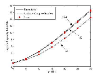
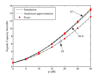
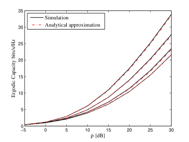
and α>0𝛼0\alpha>0 is the parameter controlling the uniformity of the powers across the antennas. Note that as α0𝛼0\alpha\rightarrow 0 the received power is dominant at the first location, as α𝛼\alpha becomes large (α1)much-greater-than𝛼1\left(\alpha\gg 1\right) the third location is dominant and as α1𝛼1\alpha\rightarrow 1 there is an even spread, as in the standard microdiversity scenario. Using these parameters, eight scenarios are given in Table I for the case of two single antenna users. In Fig. 2, we explore the capacity of scenarios S1-S4 where nR=3subscript𝑛𝑅3n_{R}=3. The capacity result in (41) agrees with the simulations for all scenarios, thus verifying the exact analysis. Furthermore, the approximation in (61) is shown to be extremely accurate. All capacity results are extremely similar except for S1, where both sources have their dominant path at the first receive antenna. Here, the system is largely overloaded (two strong signals at a single antenna) and the performance is lower. The similarity of S3 and S4 is interesting as they represent very different systems. In S3, the two users are essentially separate with the dominant channels being at different antennas. In S4, both users have power equally spread over all antennas so the users are sharing all available channels. Figure 3 follows the same pattern with S6 (the overloaded case) being lower and the other scenarios almost equivalent. In Fig. 3, the overall capacity level is reduced in comparison to Fig. 2 as ς=10𝜍10\varsigma=10 implies a weaker second source.
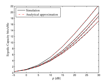
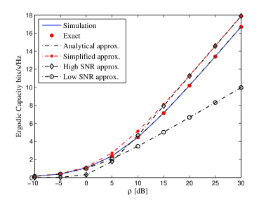
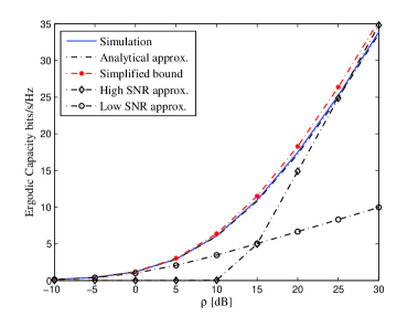
Figures 4 and 5 show results for a random drop scenario with M=nR=3,W=N=3formulae-sequence𝑀subscript𝑛𝑅3𝑊𝑁3M=n_{R}=3,W=N=3 and nR=6,M=3,W=N=6formulae-sequencesubscript𝑛𝑅6formulae-sequence𝑀3𝑊𝑁6n_{R}=6,M=3,W=N=6 respectively. In each random drop, uniform random locations are created for the users and lognormal shadow fading and path loss are considered where σSF=8subscript𝜎𝑆𝐹8\sigma_{SF}=8dB (standard deviation of shadow fading) and γ=3.5𝛾3.5\gamma=3.5 (path loss exponent). The transmit power of the sources is scaled so that all locations in the coverage area have a maximum received SNR greater than 333dB, at least 95%percent9595\% of the time. The maximum SNR is taken over the 3 BSs. Hence, each drop produces a different P𝑃P matrix and independent channels are assumed. The excellent agreement between the approximation in (61) and the simulations in both Fig. 4 and Fig. 5 is encouraging as this demonstrates the accuracy of (61) over different system sizes as well as over completely different sets of channel powers. Note that at high SNR, Fig. 5 gives much higher capacity values than Fig. 4 since there are 6 receive antenna rather than 3. In this high SNR region, the γ¯Nsuperscript¯𝛾𝑁\bar{\gamma}^{N} term in (64) dominates and capacity can be approximated by log2(1+Perm(P)γ¯N)subscript21Perm𝑃superscript¯𝛾𝑁\log_{2}\left(1+\mbox{Perm}\left(\mbox{\boldsymbol{$P$}}\right)\bar{\gamma}^{N}\right). With nR=N=3subscript𝑛𝑅𝑁3n_{R}=N=3 there are 6 cross products in Perm(P)Perm𝑃\mbox{Perm}\left(\mbox{\boldsymbol{$P$}}\right) whereas with nR=N=6subscript𝑛𝑅𝑁6n_{R}=N=6 there are 720 cross products. Hence, the bound clearly demonstrates the benefits of increased antenna numbers. In practice there is a trade-off between the costs of increased collaboration between possibly distant BSs and the resulting increase in system capacity. In Figs. 2 - 5, at low SNR the capacity is controlled by PTsubscript𝑃𝑇P_{T}. Hence, since ρ=PT/σ2𝜌subscript𝑃𝑇superscript𝜎2\rho=P_{T}/\sigma^{2}, all four drops have similar performance at low SNR and diverge at higher SNR where the channel profiles affect the results. The upper bound and associated approximations are shown in Figs. 6 and 7 both for a two user scenario (S3) and a random drop. In Fig. 6, the upper bound is shown for scenario S3 as well as the high and low SNR approximations. The results clearly show the loss in accuracy resulting from the use of the simple Jensen bound. However, the bound is quite reasonable over the whole SNR range. The low SNR approximations are quite reasonable below 0 dB and the high SNR version is as accurate as the bound above 15 dB. In Fig. 7, similar results are shown for a random drop with M=nR=6,W=N=6formulae-sequence𝑀subscript𝑛𝑅6𝑊𝑁6M=n_{R}=6,W=N=6. Here, similar patterns are observed but the low and high SNR approximations become reasonable at more widely spread SNR values. For example, the low SNR results are accurate below 0 dB and the high SNR results are poor until around 30 dB. In contrast, the upper bound is reasonable throughout. Hence, although there is a noticeable capacity error at high SNR, the cross-product coefficients in (65) and (66) are seen to explain the large majority of the ergodic capacity behavior.

TABLE I: Parameters for Figures 2 and 3
Decay Parameter
Sc. No. User 1 User 2 ς𝜍\varsigma
S1 α=0.1𝛼0.1\alpha=0.1 α=0.1𝛼0.1\alpha=0.1 1
S2 α=0.1𝛼0.1\alpha=0.1 α=1𝛼1\alpha=1 1
S3 α=0.1𝛼0.1\alpha=0.1 α=10𝛼10\alpha=10 1
S4 α=1𝛼1\alpha=1 α=1𝛼1\alpha=1 1
S5 α=0.1𝛼0.1\alpha=0.1 α=0.1𝛼0.1\alpha=0.1 10
S6 α=0.1𝛼0.1\alpha=0.1 α=1𝛼1\alpha=1 10
S7 α=0.1𝛼0.1\alpha=0.1 α=10𝛼10\alpha=10 10
S8 α=1𝛼1\alpha=1 α=0.1𝛼0.1\alpha=0.1 10

Refer to caption


Figure 2: Exact, approximated and simulated ergodic sum capacity in flat Rayleigh fading for scenarios S1-S4 with parameters: nR=3subscript𝑛𝑅3n_{R}=3, N=W=2𝑁𝑊2N=W=2 and ς=1𝜍1\varsigma=1.

Refer to caption

Figure 3: Exact, approximated and simulated ergodic sum capacity in flat Rayleigh fading for scenarios S5-S8 with parameters: nR=3subscript𝑛𝑅3n_{R}=3, N=W=2𝑁𝑊2N=W=2 and ς=10𝜍10\varsigma=10.

Refer to caption

Figure 4: Approximated and simulated ergodic sum capacity in flat Rayleigh fading for M=nR=3𝑀subscript𝑛𝑅3M=n_{R}=3, W=N=3𝑊𝑁3W=N=3 and four random drops.

Refer to caption

Figure 5: Approximated and simulated ergodic sum capacity in flat Rayleigh fading for nR=6subscript𝑛𝑅6n_{R}=6, M=3𝑀3M=3, W=N=6𝑊𝑁6W=N=6 and four random drops.

Refer to caption

Figure 6: Ergodic sum capacity in flat Rayleigh fading for scenario S3 with parameters: M=nR=3𝑀subscript𝑛𝑅3M=n_{R}=3, W=N=2𝑊𝑁2W=N=2 and ς=1𝜍1\varsigma=1.

Refer to caption

Figure 7: Ergodic sum capacity in flat Rayleigh fading for a random drop with parameters: nR=6subscript𝑛𝑅6n_{R}=6, M=3𝑀3M=3 and W=N=6𝑊𝑁6W=N=6.

VIII Conclusion

In this paper, we have studied the ergodic sum capacity of a Rayleigh fading macrodiversity MIMO-MAC. The results obtained are shown to be valid for both independent channels and correlated channels, which may occur when some of the distributed transmit/receive locations have closely spaced antennas. In particular, we derive exact results for the two-source scenario and approximate results for the general case. The approximations have a simple form and are shown to be very accurate over a wide range of channel powers. In addition, a simple upper bound is presented which demonstrates the importance of various channel power cross products in determining capacity.

Appendix A Derivation of Ibsubscript𝐼𝑏I_{b}

From (39), Ibsubscript𝐼𝑏I_{b} can be written as

Ibsubscript𝐼𝑏\displaystyle I_{b} =I~bθ1|θ1=0,absentevaluated-atsubscript~𝐼𝑏subscript𝜃1subscript𝜃10\displaystyle=\left.\frac{\partial\tilde{I}_{b}}{\partial\theta_{1}}\right|_{\theta_{1}=0}, (69)

where

I~b=00eσ2tσ2θ2i=1nR(1+tPi2+θ1Pi1Pi2+θ2Pi1)𝑑θ2𝑑t.subscript~𝐼𝑏superscriptsubscript0superscriptsubscript0superscript𝑒superscript𝜎2𝑡superscript𝜎2subscript𝜃2superscriptsubscriptproduct𝑖1subscript𝑛𝑅1𝑡subscript𝑃𝑖2subscript𝜃1subscript𝑃𝑖1subscript𝑃𝑖2subscript𝜃2subscript𝑃𝑖1differential-dsubscript𝜃2differential-d𝑡\tilde{I}_{b}=-\!\!\int_{0}^{\infty}\!\!\!\!\int_{0}^{\infty}\!\!\frac{e^{-\sigma^{2}t-\sigma^{2}\theta_{2}}}{\prod_{i=1}^{n_{R}}\left(1+tP_{i2}+\theta_{1}P_{i1}P_{i2}+\theta_{2}P_{i1}\right)}d\theta_{2}dt. (70)

From (70), Lbsubscript𝐿𝑏L_{b} becomes

Lb=00eσ2tσ2θ2i=1nR(θ1+θ2Pi2+tPi1+1Pi1Pi2)𝑑θ2𝑑t.subscript𝐿𝑏superscriptsubscript0superscriptsubscript0superscript𝑒superscript𝜎2𝑡superscript𝜎2subscript𝜃2superscriptsubscriptproduct𝑖1subscript𝑛𝑅subscript𝜃1subscript𝜃2subscript𝑃𝑖2𝑡subscript𝑃𝑖11subscript𝑃𝑖1subscript𝑃𝑖2differential-dsubscript𝜃2differential-d𝑡\displaystyle L_{b}=\int_{0}^{\infty}\!\!\!\!\int_{0}^{\infty}\!\!\!\!\frac{e^{-\sigma^{2}t-\sigma^{2}\theta_{2}}}{\prod_{i=1}^{n_{R}}\left(\theta_{1}+\frac{\theta_{2}}{P_{i2}}+\frac{t}{P_{i1}}+\frac{1}{P_{i1}P_{i2}}\right)}d\theta_{2}dt. (71)

Defining

Lbsubscript𝐿𝑏\displaystyle L_{b} =|P1P2|I~b,absentsubscript𝑃1subscript𝑃2subscript~𝐼𝑏\displaystyle=-\left|\mbox{\boldsymbol{$P$}}_{1}\mbox{\boldsymbol{$P$}}_{2}\right|\tilde{I}_{b}, (72)

we use a partial fraction expansion in θ1subscript𝜃1\theta_{1} to give

Lb=i=1nR00Ai(θ2,t)eσ2tσ2θ2(θ1+θ2Pi2+tPi1+1Pi1Pi2)𝑑θ2𝑑t,subscript𝐿𝑏superscriptsubscript𝑖1subscript𝑛𝑅superscriptsubscript0superscriptsubscript0subscript𝐴𝑖subscript𝜃2𝑡superscript𝑒superscript𝜎2𝑡superscript𝜎2subscript𝜃2subscript𝜃1subscript𝜃2subscript𝑃𝑖2𝑡subscript𝑃𝑖11subscript𝑃𝑖1subscript𝑃𝑖2differential-dsubscript𝜃2differential-d𝑡\displaystyle L_{b}=\sum_{i=1}^{n_{R}}\int_{0}^{\infty}\!\!\!\!\int_{0}^{\infty}\!\frac{A_{i}\left(\theta_{2},t\right)e^{-\sigma^{2}t-\sigma^{2}\theta_{2}}}{\left(\theta_{1}+\frac{\theta_{2}}{P_{i2}}+\frac{t}{P_{i1}}+\frac{1}{P_{i1}P_{i2}}\right)}d\theta_{2}dt, (73)

where

Ai(θ2,t)subscript𝐴𝑖subscript𝜃2𝑡\displaystyle A_{i}\left(\theta_{2},t\right) =1kinR(αikθ2+βikt+γik)absent1superscriptsubscriptproduct𝑘𝑖subscript𝑛𝑅subscript𝛼𝑖𝑘subscript𝜃2subscript𝛽𝑖𝑘𝑡subscript𝛾𝑖𝑘\displaystyle=\frac{1}{\prod_{k\neq i}^{n_{R}}\left(\alpha_{ik}\theta_{2}+\beta_{ik}t+\gamma_{ik}\right)} (74a)
αiksubscript𝛼𝑖𝑘\displaystyle\alpha_{ik} =1Pk21Pi2absent1subscript𝑃𝑘21subscript𝑃𝑖2\displaystyle=\frac{1}{P_{k2}}-\frac{1}{P_{i2}} (74b)
βiksubscript𝛽𝑖𝑘\displaystyle\beta_{ik} =1Pk11Pi1absent1subscript𝑃𝑘11subscript𝑃𝑖1\displaystyle=\frac{1}{P_{k1}}-\frac{1}{P_{i1}} (74c)
γiksubscript𝛾𝑖𝑘\displaystyle\gamma_{ik} =RkRiabsentsubscript𝑅𝑘subscript𝑅𝑖\displaystyle=R_{k}-R_{i} (74d)
Risubscript𝑅𝑖\displaystyle R_{i} =1Pi1Pi2.absent1subscript𝑃𝑖1subscript𝑃𝑖2\displaystyle=\frac{1}{P_{i1}P_{i2}}. (74e)

To compute (73), the following substitutions are employed

u=σ2t+σ2θ2𝑢superscript𝜎2𝑡superscript𝜎2subscript𝜃2\displaystyle u=\sigma^{2}t+\sigma^{2}\theta_{2} (75a)
vi=tPi1+θ2Pi2.subscript𝑣𝑖𝑡subscript𝑃𝑖1subscript𝜃2subscript𝑃𝑖2\displaystyle v_{i}=\frac{t}{P_{i1}}+\frac{\theta_{2}}{P_{i2}}. (75b)

The Jacobian of the transformation in (75b) can be calculated as

Ji=σ2(1Pi21Pi1).subscript𝐽𝑖superscript𝜎21subscript𝑃𝑖21subscript𝑃𝑖1\displaystyle J_{i}=\sigma^{2}\left(\frac{1}{P_{i2}}-\frac{1}{P_{i1}}\right). (76)

Substituting (75b) and (76) in (73) gives

Lb=i=1nR0uPi1σ2uPi2σ2Ai(u,vi)euJi(vi+θ1+Ri)𝑑vi𝑑u,subscript𝐿𝑏superscriptsubscript𝑖1subscript𝑛𝑅superscriptsubscript0superscriptsubscript𝑢subscript𝑃𝑖1superscript𝜎2𝑢subscript𝑃𝑖2superscript𝜎2subscript𝐴𝑖𝑢subscript𝑣𝑖superscript𝑒𝑢subscript𝐽𝑖subscript𝑣𝑖subscript𝜃1subscript𝑅𝑖differential-dsubscript𝑣𝑖differential-d𝑢\displaystyle L_{b}=\sum_{i=1}^{n_{R}}\int_{0}^{\infty}\!\!\!\!\int_{\frac{u}{P_{i1}\sigma^{2}}}^{\frac{u}{P_{i2}\sigma^{2}}}\frac{A_{i}\left(u,v_{i}\right)e^{-u}}{J_{i}\left(v_{i}+\theta_{1}+R_{i}\right)}dv_{i}du, (77)

where

Ai(u,vi)subscript𝐴𝑖𝑢subscript𝑣𝑖\displaystyle A_{i}\left(u,v_{i}\right) =1kinR(aikvi+biku+γik)absent1superscriptsubscriptproduct𝑘𝑖subscript𝑛𝑅subscript𝑎𝑖𝑘subscript𝑣𝑖subscript𝑏𝑖𝑘𝑢subscript𝛾𝑖𝑘\displaystyle=\frac{1}{\prod_{k\neq i}^{n_{R}}\left(a_{ik}v_{i}+b_{ik}u+\gamma_{ik}\right)} (78a)
aiksubscript𝑎𝑖𝑘\displaystyle a_{ik} =σ2Ji(αikβik)absentsuperscript𝜎2subscript𝐽𝑖subscript𝛼𝑖𝑘subscript𝛽𝑖𝑘\displaystyle=\frac{\sigma^{2}}{J_{i}}\left(\alpha_{ik}-\beta_{ik}\right) (78b)
biksubscript𝑏𝑖𝑘\displaystyle b_{ik} =1Ji(βikPi2αikPi1).absent1subscript𝐽𝑖subscript𝛽𝑖𝑘subscript𝑃𝑖2subscript𝛼𝑖𝑘subscript𝑃𝑖1\displaystyle=\frac{1}{J_{i}}\left(\frac{\beta_{ik}}{P_{i2}}-\frac{\alpha_{ik}}{P_{i1}}\right). (78c)

The term Ai(u,vi)subscript𝐴𝑖𝑢subscript𝑣𝑖A_{i}\left(u,v_{i}\right) in (78a) can be written as a summation using partial fractions, to give

Ai(u,vi)subscript𝐴𝑖𝑢subscript𝑣𝑖\displaystyle A_{i}\left(u,v_{i}\right) =kinRBik(u)vi+qiku+rik,absentsuperscriptsubscript𝑘𝑖subscript𝑛𝑅subscript𝐵𝑖𝑘𝑢subscript𝑣𝑖subscript𝑞𝑖𝑘𝑢subscript𝑟𝑖𝑘\displaystyle=\sum_{k\neq i}^{n_{R}}\frac{B_{ik}\left(u\right)}{v_{i}+q_{ik}u+r_{ik}}, (79)

where

Bik(u)subscript𝐵𝑖𝑘𝑢\displaystyle B_{ik}\left(u\right) =(aik)nR3li,knR(ciklu+dikl)absentsuperscriptsubscript𝑎𝑖𝑘subscript𝑛𝑅3superscriptsubscriptproduct𝑙𝑖𝑘subscript𝑛𝑅subscript𝑐𝑖𝑘𝑙𝑢subscript𝑑𝑖𝑘𝑙\displaystyle=\frac{\left(a_{ik}\right)^{n_{R}-3}}{\prod_{l\neq i,k}^{n_{R}}\left(c_{ikl}u+d_{ikl}\right)} (80a)
ciklsubscript𝑐𝑖𝑘𝑙\displaystyle c_{ikl} =bilaikailbikabsentsubscript𝑏𝑖𝑙subscript𝑎𝑖𝑘subscript𝑎𝑖𝑙subscript𝑏𝑖𝑘\displaystyle=b_{il}a_{ik}-a_{il}b_{ik} (80b)
diklsubscript𝑑𝑖𝑘𝑙\displaystyle d_{ikl} =aikγilγikailabsentsubscript𝑎𝑖𝑘subscript𝛾𝑖𝑙subscript𝛾𝑖𝑘subscript𝑎𝑖𝑙\displaystyle=a_{ik}\gamma_{il}-\gamma_{ik}a_{il} (80c)
qiksubscript𝑞𝑖𝑘\displaystyle q_{ik} =bikaikabsentsubscript𝑏𝑖𝑘subscript𝑎𝑖𝑘\displaystyle=\frac{b_{ik}}{a_{ik}} (80d)
riksubscript𝑟𝑖𝑘\displaystyle r_{ik} =γikaik.absentsubscript𝛾𝑖𝑘subscript𝑎𝑖𝑘\displaystyle=\frac{\gamma_{ik}}{a_{ik}}. (80e)

Substituting (79) in (77) and simplifying gives

Lb=i=1nRsubscript𝐿𝑏superscriptsubscript𝑖1subscript𝑛𝑅\displaystyle\!\!\!\!\!L_{b}=\sum_{i=1}^{n_{R}} kinR0uPi1σ2uPi2σ2Bik(u)euJidvidu(vi+θ1+Ri)(vi+qiku+rik).superscriptsubscript𝑘𝑖subscript𝑛𝑅superscriptsubscript0superscriptsubscript𝑢subscript𝑃𝑖1superscript𝜎2𝑢subscript𝑃𝑖2superscript𝜎2subscript𝐵𝑖𝑘𝑢superscript𝑒𝑢subscript𝐽𝑖𝑑subscript𝑣𝑖𝑑𝑢subscript𝑣𝑖subscript𝜃1subscript𝑅𝑖subscript𝑣𝑖subscript𝑞𝑖𝑘𝑢subscript𝑟𝑖𝑘\displaystyle\sum_{k\neq i}^{n_{R}}\int_{0}^{\infty}\int_{\frac{u}{P_{i1}\sigma^{2}}}^{\frac{u}{P_{i2}\sigma^{2}}}\frac{B_{ik}\left(u\right)e^{-u}}{J_{i}}\left.\frac{dv_{i}du}{\left(v_{i}+\theta_{1}+R_{i}\right)\left(v_{i}+q_{ik}u+r_{ik}\right)}\right.. (81)

First, we integrate over visubscript𝑣𝑖v_{i} in (81) to give

Lb=i=1nRsubscript𝐿𝑏superscriptsubscript𝑖1subscript𝑛𝑅\displaystyle\!\!\!\!\!\!\!L_{b}=\sum_{i=1}^{n_{R}} kinR0Cik(u,θ1)euJiln[(uPi2σ2+θ1+Ri)(λiku+rik)(uPi1σ2+θ1+Ri)(μiku+rik)]𝑑u,superscriptsubscript𝑘𝑖subscript𝑛𝑅superscriptsubscript0subscript𝐶𝑖𝑘𝑢subscript𝜃1superscript𝑒𝑢subscript𝐽𝑖𝑢subscript𝑃𝑖2superscript𝜎2subscript𝜃1subscript𝑅𝑖subscript𝜆𝑖𝑘𝑢subscript𝑟𝑖𝑘𝑢subscript𝑃𝑖1superscript𝜎2subscript𝜃1subscript𝑅𝑖subscript𝜇𝑖𝑘𝑢subscript𝑟𝑖𝑘differential-d𝑢\displaystyle\sum_{k\neq i}^{n_{R}}\int_{0}^{\infty}\frac{C_{ik}\left(u,\theta_{1}\right)e^{-u}}{J_{i}}\ln\left[\frac{\left(\frac{u}{P_{i2}\sigma^{2}}+\theta_{1}+R_{i}\right)\!\!\left(\lambda_{ik}u+r_{ik}\right)}{\left(\frac{u}{P_{i1}\sigma^{2}}+\theta_{1}+R_{i}\right)\!\!\left(\mu_{ik}u+r_{ik}\right)}\right]du, (82)

where

Cik(u,θ1)subscript𝐶𝑖𝑘𝑢subscript𝜃1\displaystyle C_{ik}\left(u,\theta_{1}\right) =Bik(u)qiku+rikθ1Riabsentsubscript𝐵𝑖𝑘𝑢subscript𝑞𝑖𝑘𝑢subscript𝑟𝑖𝑘subscript𝜃1subscript𝑅𝑖\displaystyle=\frac{B_{ik}\left(u\right)}{q_{ik}u+r_{ik}-\theta_{1}-R_{i}} (83a)
λiksubscript𝜆𝑖𝑘\displaystyle\lambda_{ik} =1Pi1σ2+qikabsent1subscript𝑃𝑖1superscript𝜎2subscript𝑞𝑖𝑘\displaystyle=\frac{1}{P_{i1}\sigma^{2}}+q_{ik} (83b)
μiksubscript𝜇𝑖𝑘\displaystyle\mu_{ik} =1Pi2σ2+qik.absent1subscript𝑃𝑖2superscript𝜎2subscript𝑞𝑖𝑘\displaystyle=\frac{1}{P_{i2}\sigma^{2}}+q_{ik}. (83c)

Let

Dik(u,θ1)subscript𝐷𝑖𝑘𝑢subscript𝜃1\displaystyle D_{ik}\left(u,\theta_{1}\right) =ln[(uPi2σ2+θ1+Ri)(λiku+rik)(uPi1σ2+θ1+Ri)(μiku+rik)],absent𝑢subscript𝑃𝑖2superscript𝜎2subscript𝜃1subscript𝑅𝑖subscript𝜆𝑖𝑘𝑢subscript𝑟𝑖𝑘𝑢subscript𝑃𝑖1superscript𝜎2subscript𝜃1subscript𝑅𝑖subscript𝜇𝑖𝑘𝑢subscript𝑟𝑖𝑘\displaystyle=\ln\left[\frac{\left(\frac{u}{P_{i2}\sigma^{2}}+\theta_{1}+R_{i}\right)\!\!\left(\lambda_{ik}u+r_{ik}\right)}{\left(\frac{u}{P_{i1}\sigma^{2}}+\theta_{1}+R_{i}\right)\!\!\left(\mu_{ik}u+r_{ik}\right)}\right], (84a)

then Bik(u)subscript𝐵𝑖𝑘𝑢B_{ik}\left(u\right) in (80a) can be rewritten as the summation

Bik(u)=li,knRξiklciklu+dikl,subscript𝐵𝑖𝑘𝑢superscriptsubscript𝑙𝑖𝑘subscript𝑛𝑅subscript𝜉𝑖𝑘𝑙subscript𝑐𝑖𝑘𝑙𝑢subscript𝑑𝑖𝑘𝑙\displaystyle B_{ik}\left(u\right)=\sum_{l\neq i,k}^{n_{R}}\frac{\xi_{ikl}}{c_{ikl}u+d_{ikl}}, (85)

where

ξikl=(aikcikl)nR3zi,k,lnR(dikzciklcikzdikl).subscript𝜉𝑖𝑘𝑙superscriptsubscript𝑎𝑖𝑘subscript𝑐𝑖𝑘𝑙subscript𝑛𝑅3superscriptsubscriptproduct𝑧𝑖𝑘𝑙subscript𝑛𝑅subscript𝑑𝑖𝑘𝑧subscript𝑐𝑖𝑘𝑙subscript𝑐𝑖𝑘𝑧subscript𝑑𝑖𝑘𝑙\displaystyle\xi_{ikl}=\frac{\left(a_{ik}c_{ikl}\right)^{n_{R}-3}}{\prod_{z\neq i,k,l}^{n_{R}}\left(d_{ikz}c_{ikl}-c_{ikz}d_{ikl}\right)}. (86)

Substituting (85) and (83c) in (82) gives

Lb=i=1nRsubscript𝐿𝑏superscriptsubscript𝑖1subscript𝑛𝑅\displaystyle L_{b}=\sum_{i=1}^{n_{R}} kinRli,knR0Dik(u,θ1)ξiklJidu(ciklu+dikl)(qiku+rikθ1Ri).superscriptsubscript𝑘𝑖subscript𝑛𝑅superscriptsubscript𝑙𝑖𝑘subscript𝑛𝑅superscriptsubscript0subscript𝐷𝑖𝑘𝑢subscript𝜃1subscript𝜉𝑖𝑘𝑙subscript𝐽𝑖𝑑𝑢subscript𝑐𝑖𝑘𝑙𝑢subscript𝑑𝑖𝑘𝑙subscript𝑞𝑖𝑘𝑢subscript𝑟𝑖𝑘subscript𝜃1subscript𝑅𝑖\displaystyle\sum_{k\neq i}^{n_{R}}\sum_{l\neq i,k}^{n_{R}}\int_{0}^{\infty}D_{ik}\left(u,\theta_{1}\right)\frac{\xi_{ikl}}{J_{i}}\frac{du}{\left(c_{ikl}u+d_{ikl}\right)\left(q_{ik}u+r_{ik}-\theta_{1}-R_{i}\right)}. (87)

Equation (87) can be further simplified to give

Lbsubscript𝐿𝑏\displaystyle L_{b} =i=1nRkinRli,knRξikl(MbiklNbikl)Ji,absentsuperscriptsubscript𝑖1subscript𝑛𝑅superscriptsubscript𝑘𝑖subscript𝑛𝑅superscriptsubscript𝑙𝑖𝑘subscript𝑛𝑅subscript𝜉𝑖𝑘𝑙subscript𝑀subscript𝑏𝑖𝑘𝑙subscript𝑁subscript𝑏𝑖𝑘𝑙subscript𝐽𝑖\displaystyle=\sum_{i=1}^{n_{R}}\sum_{k\neq i}^{n_{R}}\sum_{l\neq i,k}^{n_{R}}\frac{\xi_{ikl}\left(M_{b_{ikl}}-N_{b_{ikl}}\right)}{J_{i}}, (88)

where

Mbiklsubscript𝑀subscript𝑏𝑖𝑘𝑙\displaystyle M_{b_{ikl}} =0Dik(u,θ1)f1(θ1)du(u+εikl),absentsuperscriptsubscript0subscript𝐷𝑖𝑘𝑢subscript𝜃1subscript𝑓1subscript𝜃1𝑑𝑢𝑢subscript𝜀𝑖𝑘𝑙\displaystyle=\int_{0}^{\infty}\frac{D_{ik}\left(u,\theta_{1}\right)}{f_{1}\left(\theta_{1}\right)}\frac{du}{\left(u+\varepsilon_{ikl}\right)}, (89)
Nbiklsubscript𝑁subscript𝑏𝑖𝑘𝑙\displaystyle N_{b_{ikl}} =0Dik(u,θ1)f1(θ1)du(u+f2(θ1)),absentsuperscriptsubscript0subscript𝐷𝑖𝑘𝑢subscript𝜃1subscript𝑓1subscript𝜃1𝑑𝑢𝑢subscript𝑓2subscript𝜃1\displaystyle=\int_{0}^{\infty}\frac{D_{ik}\left(u,\theta_{1}\right)}{f_{1}\left(\theta_{1}\right)}\frac{du}{\left(u+f_{2}\left(\theta_{1}\right)\right)}, (90)

and εikl=dikl/ciklsubscript𝜀𝑖𝑘𝑙subscript𝑑𝑖𝑘𝑙subscript𝑐𝑖𝑘𝑙\varepsilon_{ikl}=d_{ikl}/c_{ikl}. Next, we introduce the following linear functions of θ1subscript𝜃1\theta_{1}:

f1(θ1)subscript𝑓1subscript𝜃1\displaystyle f_{1}\left(\theta_{1}\right) =niklciklθ1absentsubscript𝑛𝑖𝑘𝑙subscript𝑐𝑖𝑘𝑙subscript𝜃1\displaystyle=n_{ikl}-c_{ikl}\theta_{1} (91)
f2(θ1)subscript𝑓2subscript𝜃1\displaystyle f_{2}\left(\theta_{1}\right) =miklθ1qik,absentsubscript𝑚𝑖𝑘𝑙subscript𝜃1subscript𝑞𝑖𝑘\displaystyle=m_{ikl}-\frac{\theta_{1}}{q_{ik}}, (92)

where

niklsubscript𝑛𝑖𝑘𝑙\displaystyle n_{ikl} =rikcikldiklqikciklRiabsentsubscript𝑟𝑖𝑘subscript𝑐𝑖𝑘𝑙subscript𝑑𝑖𝑘𝑙subscript𝑞𝑖𝑘subscript𝑐𝑖𝑘𝑙subscript𝑅𝑖\displaystyle=r_{ik}c_{ikl}-d_{ikl}q_{ik}-\frac{c_{ikl}}{R_{i}} (93)
miklsubscript𝑚𝑖𝑘𝑙\displaystyle m_{ikl} =γikbik1qikRi.absentsubscript𝛾𝑖𝑘subscript𝑏𝑖𝑘1subscript𝑞𝑖𝑘subscript𝑅𝑖\displaystyle=\frac{\gamma_{ik}}{b_{ik}}-\frac{1}{q_{ik}R_{i}}. (94)

Next, we can differentiate Mbiklsubscript𝑀subscript𝑏𝑖𝑘𝑙M_{b_{ikl}} and Nbiklsubscript𝑁subscript𝑏𝑖𝑘𝑙N_{b_{ikl}} and integrate over u𝑢u to give the final result along with (69) and (72). Hence, from (91) and (84a) we get (95).

θ1[Dik(u,θ1)f1(θ1)]θ1=0=ciklnikl2subscript𝜃1subscriptdelimited-[]subscript𝐷𝑖𝑘𝑢subscript𝜃1subscript𝑓1subscript𝜃1subscript𝜃10subscript𝑐𝑖𝑘𝑙superscriptsubscript𝑛𝑖𝑘𝑙2\displaystyle\frac{\partial}{\partial\theta_{1}}\left[\frac{D_{ik}\left(u,\theta_{1}\right)}{f_{1}\left(\theta_{1}\right)}\right]_{\theta_{1}=0}\!=\!\frac{c_{ikl}}{n_{ikl}^{2}} ln[(uPi2σ2+Ri)(λiku+rik)(uPi1σ2+Ri)(μiku+rik)]+1nikl[Pi2σ2(u+σ2Pi1)Pi1σ2(u+σ2Pi2)]𝑢subscript𝑃𝑖2superscript𝜎2subscript𝑅𝑖subscript𝜆𝑖𝑘𝑢subscript𝑟𝑖𝑘𝑢subscript𝑃𝑖1superscript𝜎2subscript𝑅𝑖subscript𝜇𝑖𝑘𝑢subscript𝑟𝑖𝑘1subscript𝑛𝑖𝑘𝑙delimited-[]subscript𝑃𝑖2superscript𝜎2𝑢superscript𝜎2subscript𝑃𝑖1subscript𝑃𝑖1superscript𝜎2𝑢superscript𝜎2subscript𝑃𝑖2\displaystyle\ln\left[\frac{\left(\frac{u}{P_{i2}\sigma^{2}}+R_{i}\right)\left(\lambda_{ik}u+r_{ik}\right)}{\left(\frac{u}{P_{i1}\sigma^{2}}+R_{i}\right)\left(\mu_{ik}u+r_{ik}\right)}\right]+\frac{1}{n_{ikl}}\left[\frac{P_{i2}\sigma^{2}}{\left(u+\frac{\sigma^{2}}{P_{i1}}\right)}-\frac{P_{i1}\sigma^{2}}{\left(u+\frac{\sigma^{2}}{P_{i2}}\right)}\right] (95)
M~biklsubscript~𝑀subscript𝑏𝑖𝑘𝑙\displaystyle\tilde{M}_{b_{ikl}} =Mbiklθ1|θ1=0=0θ1[Dik(u,θ1)f1(θ1)]θ1=0du(u+eikl)absentevaluated-atsubscript𝑀subscript𝑏𝑖𝑘𝑙subscript𝜃1subscript𝜃10superscriptsubscript0subscript𝜃1subscriptdelimited-[]subscript𝐷𝑖𝑘𝑢subscript𝜃1subscript𝑓1subscript𝜃1subscript𝜃10𝑑𝑢𝑢subscript𝑒𝑖𝑘𝑙\displaystyle=\left.\frac{\partial M_{b_{ikl}}}{\partial\theta_{1}}\right|_{\theta_{1}=0}=\int_{0}^{\infty}\frac{\partial}{\partial\theta_{1}}\left[\frac{D_{ik}\left(u,\theta_{1}\right)}{f_{1}\left(\theta_{1}\right)}\right]_{\theta_{1}=0}\frac{du}{\left(u+e_{ikl}\right)} (96)
N~biklsubscript~𝑁subscript𝑏𝑖𝑘𝑙\displaystyle\tilde{N}_{b_{ikl}} =Nbiklθ1|θ1=0=0θ1[Dik(u,θ1)f1(θ1)]θ1=0du(u+mikl)+0[Dik(u,θ1)f1(θ1)]θ1=01/qik(u+mikl)2𝑑uabsentevaluated-atsubscript𝑁subscript𝑏𝑖𝑘𝑙subscript𝜃1subscript𝜃10superscriptsubscript0subscript𝜃1subscriptdelimited-[]subscript𝐷𝑖𝑘𝑢subscript𝜃1subscript𝑓1subscript𝜃1subscript𝜃10𝑑𝑢𝑢subscript𝑚𝑖𝑘𝑙superscriptsubscript0subscriptdelimited-[]subscript𝐷𝑖𝑘𝑢subscript𝜃1subscript𝑓1subscript𝜃1subscript𝜃101subscript𝑞𝑖𝑘superscript𝑢subscript𝑚𝑖𝑘𝑙2differential-d𝑢\displaystyle=\left.\frac{\partial N_{b_{ikl}}}{\partial\theta_{1}}\right|_{\theta_{1}=0}=\int_{0}^{\infty}\frac{\partial}{\partial\theta_{1}}\left[\frac{D_{ik}\left(u,\theta_{1}\right)}{f_{1}\left(\theta_{1}\right)}\right]_{\theta_{1}=0}\frac{du}{\left(u+m_{ikl}\right)}+\int_{0}^{\infty}\left[\frac{D_{ik}\left(u,\theta_{1}\right)}{f_{1}\left(\theta_{1}\right)}\right]_{\theta_{1}=0}\frac{1/q_{ik}}{\left(u+m_{ikl}\right)^{2}}du (97)
M~biklsubscript~𝑀subscript𝑏𝑖𝑘𝑙\displaystyle\tilde{M}_{b_{ikl}} =ciklnikl2[H1(Ri,εikl,1Pi2σ2)+H1(rik,εikl,λik)H1(Ri,εikl,1Pi1σ2)H1(rik,εikl,μik)]absentsubscript𝑐𝑖𝑘𝑙superscriptsubscript𝑛𝑖𝑘𝑙2delimited-[]subscript𝐻1subscript𝑅𝑖subscript𝜀𝑖𝑘𝑙1subscript𝑃𝑖2superscript𝜎2subscript𝐻1subscript𝑟𝑖𝑘subscript𝜀𝑖𝑘𝑙subscript𝜆𝑖𝑘subscript𝐻1subscript𝑅𝑖subscript𝜀𝑖𝑘𝑙1subscript𝑃𝑖1superscript𝜎2subscript𝐻1subscript𝑟𝑖𝑘subscript𝜀𝑖𝑘𝑙subscript𝜇𝑖𝑘\displaystyle=\frac{c_{ikl}}{n_{ikl}^{2}}\left[H_{1}\left(R_{i},\varepsilon_{ikl},\frac{1}{P_{i2}\sigma^{2}}\right)+H_{1}\left(r_{ik},\varepsilon_{ikl},\lambda_{ik}\right)-H_{1}\left(R_{i},\varepsilon_{ikl},\frac{1}{P_{i1}\sigma^{2}}\right)-H_{1}\left(r_{ik},\varepsilon_{ikl},\mu_{ik}\right)\right]
+εiklnikl[eσ2Pi1E1(σ2Pi1)eεiklE1(εikl)]εikl′′nikl[eσ2Pi2E1(σ2Pi2)eεiklE1(εikl)],subscriptsuperscript𝜀𝑖𝑘𝑙subscript𝑛𝑖𝑘𝑙delimited-[]superscript𝑒superscript𝜎2subscript𝑃𝑖1subscript𝐸1superscript𝜎2subscript𝑃𝑖1superscript𝑒subscript𝜀𝑖𝑘𝑙subscript𝐸1subscript𝜀𝑖𝑘𝑙subscriptsuperscript𝜀′′𝑖𝑘𝑙subscript𝑛𝑖𝑘𝑙delimited-[]superscript𝑒superscript𝜎2subscript𝑃𝑖2subscript𝐸1superscript𝜎2subscript𝑃𝑖2superscript𝑒subscript𝜀𝑖𝑘𝑙subscript𝐸1subscript𝜀𝑖𝑘𝑙\displaystyle+\frac{\varepsilon^{\prime}_{ikl}}{n_{ikl}}\left[e^{\frac{\sigma^{2}}{P_{i1}}}E_{1}\left(\frac{\sigma^{2}}{P_{i1}}\right)-e^{\varepsilon_{ikl}}E_{1}\left(\varepsilon_{ikl}\right)\right]-\frac{\varepsilon^{\prime\prime}_{ikl}}{n_{ikl}}\left[e^{\frac{\sigma^{2}}{P_{i2}}}E_{1}\left(\frac{\sigma^{2}}{P_{i2}}\right)-e^{\varepsilon_{ikl}}E_{1}\left(\varepsilon_{ikl}\right)\right], (98)
N~biklsubscript~𝑁subscript𝑏𝑖𝑘𝑙\displaystyle\tilde{N}_{b_{ikl}} =ciklnikl2qik[H2(Ri,mikl,1Pi2σ2)+H2(rik,mikl,λik)H2(Ri,mikl,1Pi1σ2)H2(rik,mikl,μik)]absentsubscript𝑐𝑖𝑘𝑙superscriptsubscript𝑛𝑖𝑘𝑙2subscript𝑞𝑖𝑘delimited-[]subscript𝐻2subscript𝑅𝑖subscript𝑚𝑖𝑘𝑙1subscript𝑃𝑖2superscript𝜎2subscript𝐻2subscript𝑟𝑖𝑘subscript𝑚𝑖𝑘𝑙subscript𝜆𝑖𝑘subscript𝐻2subscript𝑅𝑖subscript𝑚𝑖𝑘𝑙1subscript𝑃𝑖1superscript𝜎2subscript𝐻2subscript𝑟𝑖𝑘subscript𝑚𝑖𝑘𝑙subscript𝜇𝑖𝑘\displaystyle=\frac{c_{ikl}}{n_{ikl}^{2}q_{ik}}\left[H_{2}\left(R_{i},m_{ikl},\frac{1}{P_{i2}\sigma^{2}}\right)+H_{2}\left(r_{ik},m_{ikl},\lambda_{ik}\right)-H_{2}\left(R_{i},m_{ikl},\frac{1}{P_{i1}\sigma^{2}}\right)-H_{2}\left(r_{ik},m_{ikl},\mu_{ik}\right)\right]
+ciklnikl2[H1(Ri,mikl,1Pi2σ2)+H1(rik,mikl,λik)H1(Ri,mikl,1Pi1σ2)H1(rik,mikl,μik)]subscript𝑐𝑖𝑘𝑙superscriptsubscript𝑛𝑖𝑘𝑙2delimited-[]subscript𝐻1subscript𝑅𝑖subscript𝑚𝑖𝑘𝑙1subscript𝑃𝑖2superscript𝜎2subscript𝐻1subscript𝑟𝑖𝑘subscript𝑚𝑖𝑘𝑙subscript𝜆𝑖𝑘subscript𝐻1subscript𝑅𝑖subscript𝑚𝑖𝑘𝑙1subscript𝑃𝑖1superscript𝜎2subscript𝐻1subscript𝑟𝑖𝑘subscript𝑚𝑖𝑘𝑙subscript𝜇𝑖𝑘\displaystyle+\frac{c_{ikl}}{n_{ikl}^{2}}\left[H_{1}\left(R_{i},m_{ikl},\frac{1}{P_{i2}\sigma^{2}}\right)+H_{1}\left(r_{ik},m_{ikl},\lambda_{ik}\right)-H_{1}\left(R_{i},m_{ikl},\frac{1}{P_{i1}\sigma^{2}}\right)-H_{1}\left(r_{ik},m_{ikl},\mu_{ik}\right)\right]
+miklnikl[eσ2Pi1E1(σ2Pi1)emiklE1(mikl)]mikl′′nikl[eσ2Pi2E1(σ2Pi2)emiklE1(mikl)],subscriptsuperscript𝑚𝑖𝑘𝑙subscript𝑛𝑖𝑘𝑙delimited-[]superscript𝑒superscript𝜎2subscript𝑃𝑖1subscript𝐸1superscript𝜎2subscript𝑃𝑖1superscript𝑒subscript𝑚𝑖𝑘𝑙subscript𝐸1subscript𝑚𝑖𝑘𝑙subscriptsuperscript𝑚′′𝑖𝑘𝑙subscript𝑛𝑖𝑘𝑙delimited-[]superscript𝑒superscript𝜎2subscript𝑃𝑖2subscript𝐸1superscript𝜎2subscript𝑃𝑖2superscript𝑒subscript𝑚𝑖𝑘𝑙subscript𝐸1subscript𝑚𝑖𝑘𝑙\displaystyle+\frac{m^{\prime}_{ikl}}{n_{ikl}}\left[e^{\frac{\sigma^{2}}{P_{i1}}}E_{1}\left(\frac{\sigma^{2}}{P_{i1}}\right)-e^{m_{ikl}}E_{1}\left(m_{ikl}\right)\right]-\frac{m^{\prime\prime}_{ikl}}{n_{ikl}}\left[e^{\frac{\sigma^{2}}{P_{i2}}}E_{1}\left(\frac{\sigma^{2}}{P_{i2}}\right)-e^{m_{ikl}}E_{1}\left(m_{ikl}\right)\right], (99)

Substituting (95) in (89) and (90) we get (96) and (97). (96) and (97) can be solved in closed form to give (98) and (99), where we have used the two integrals defined as follows

H1(a,b,c)subscript𝐻1𝑎𝑏𝑐\displaystyle H_{1}\left(a,b,c\right) =0etln(ct+a)t+b𝑑tabsentsuperscriptsubscript0superscript𝑒𝑡𝑐𝑡𝑎𝑡𝑏differential-d𝑡\displaystyle=\int_{0}^{\infty}\frac{e^{-t}\ln\left(ct+a\right)}{t+b}dt (100)
H2(a,b,c)subscript𝐻2𝑎𝑏𝑐\displaystyle H_{2}\left(a,b,c\right) =0etln(ct+a)(t+b)2𝑑tabsentsuperscriptsubscript0superscript𝑒𝑡𝑐𝑡𝑎superscript𝑡𝑏2differential-d𝑡\displaystyle=\int_{0}^{\infty}\frac{e^{-t}\ln\left(ct+a\right)}{\left(t+b\right)^{2}}dt (101)

and the constants are given by

εikl=1(εiklσ2Pi1),εikl′′subscriptsuperscript𝜀𝑖𝑘𝑙1subscript𝜀𝑖𝑘𝑙superscript𝜎2subscript𝑃𝑖1subscriptsuperscript𝜀′′𝑖𝑘𝑙\displaystyle\varepsilon^{\prime}_{ikl}=\frac{1}{\left(\varepsilon_{ikl}-\frac{\sigma^{2}}{P_{i1}}\right)},\quad\varepsilon^{\prime\prime}_{ikl} =1(εiklσ2Pi2),absent1subscript𝜀𝑖𝑘𝑙superscript𝜎2subscript𝑃𝑖2\displaystyle=\frac{1}{\left(\varepsilon_{ikl}-\frac{\sigma^{2}}{P_{i2}}\right)},
mikl=1(miklσ2Pi1),mikl′′subscriptsuperscript𝑚𝑖𝑘𝑙1subscript𝑚𝑖𝑘𝑙superscript𝜎2subscript𝑃𝑖1subscriptsuperscript𝑚′′𝑖𝑘𝑙\displaystyle m^{\prime}_{ikl}=\frac{1}{\left(m_{ikl}-\frac{\sigma^{2}}{P_{i1}}\right)},\quad m^{\prime\prime}_{ikl} =1(miklσ2Pi2).absent1subscript𝑚𝑖𝑘𝑙superscript𝜎2subscript𝑃𝑖2\displaystyle=\frac{1}{\left(m_{ikl}-\frac{\sigma^{2}}{P_{i2}}\right)}.

Both H1subscript𝐻1H_{1} and H2subscript𝐻2H_{2} can be solved in closed form as

H1(a,b,c)=eb[E1(b)lnc+D1(acb,b)],subscript𝐻1𝑎𝑏𝑐superscript𝑒𝑏delimited-[]subscript𝐸1𝑏𝑐subscript𝐷1𝑎𝑐𝑏𝑏H_{1}\left(a,b,c\right)=e^{b}\left[E_{1}\left(b\right)\ln c+D_{1}\left(\frac{a}{c}-b,b\right)\right],
H2(a,b,c)=lnc[1bebE1(b)]2ebD1(acb,b)+1(acb)[ebE1(b)eacE1(ac)],subscript𝐻2𝑎𝑏𝑐𝑐delimited-[]1𝑏superscript𝑒𝑏subscript𝐸1𝑏2superscript𝑒𝑏subscript𝐷1𝑎𝑐𝑏𝑏1𝑎𝑐𝑏delimited-[]superscript𝑒𝑏subscript𝐸1𝑏superscript𝑒𝑎𝑐subscript𝐸1𝑎𝑐H_{2}\left(a,b,c\right)=\ln c\left[\frac{1}{b}-e^{b}E_{1}\left(b\right)\right]-2e^{b}D_{1}\left(\frac{a}{c}-b,b\right)+\frac{1}{\left(\frac{a}{c}-b\right)}\left[e^{b}E_{1}\left(b\right)-e^{\frac{a}{c}}E_{1}\left(\frac{a}{c}\right)\right],

where D1(a,b)subscript𝐷1𝑎𝑏D_{1}(a,b) is defined by

D1(a,b)=betln(t+a)t𝑑t,forb0.formulae-sequencesubscript𝐷1𝑎𝑏superscriptsubscript𝑏superscript𝑒𝑡𝑡𝑎𝑡differential-d𝑡for𝑏0D_{1}(a,b)=\int_{b}^{\infty}\frac{e^{-t}\ln\left(t+a\right)}{t}dt,\hskip 14.22636pt\mbox{for}\hskip 14.22636ptb\neq 0.

Appendix B Calculation of E{|σ2I+H~kHH~k|}𝐸superscript𝜎2𝐼superscriptsubscript~𝐻𝑘𝐻subscript~𝐻𝑘E\left\{\left|\sigma^{2}\mbox{\boldsymbol{$I$}}+\tilde{\mbox{\boldsymbol{$H$}}}_{k}^{H}\tilde{\mbox{\boldsymbol{$H$}}}_{k}\right|\right\}

Let λ1,λ2,,λk1subscript𝜆1subscript𝜆2subscript𝜆𝑘1\lambda_{1},\lambda_{2},\dots,\lambda_{k-1} be the ordered eigenvalues of H~kHH~ksuperscriptsubscript~𝐻𝑘𝐻subscript~𝐻𝑘\tilde{\mbox{\boldsymbol{$H$}}}_{k}^{H}\tilde{\mbox{\boldsymbol{$H$}}}_{k}. Since nR(k1)subscript𝑛𝑅𝑘1n_{R}\geq\left(k-1\right), all eigenvalues are non zero. Then,

E{|σ2I+H~kHH~k|}𝐸superscript𝜎2𝐼superscriptsubscript~𝐻𝑘𝐻subscript~𝐻𝑘\displaystyle E\left\{\left|\sigma^{2}\mbox{\boldsymbol{$I$}}+\tilde{\mbox{\boldsymbol{$H$}}}_{k}^{H}\tilde{\mbox{\boldsymbol{$H$}}}_{k}\right|\right\} =E{i=1k1(σ2+λi)}absent𝐸superscriptsubscriptproduct𝑖1𝑘1superscript𝜎2subscript𝜆𝑖\displaystyle=E\left\{\prod_{i=1}^{k-1}\left(\sigma^{2}+\lambda_{i}\right)\right\}
=E{i=0k1Tri(H~kHH~k)(σ2)ki1},absent𝐸superscriptsubscript𝑖0𝑘1subscriptTr𝑖superscriptsubscript~𝐻𝑘𝐻subscript~𝐻𝑘superscriptsuperscript𝜎2𝑘𝑖1\displaystyle=\!E\!\left\{\sum_{i=0}^{k-1}\mbox{Tr}_{i}\!\left(\tilde{\mbox{\boldsymbol{$H$}}}_{k}^{H}\tilde{\mbox{\boldsymbol{$H$}}}_{k}\right)\left(\sigma^{2}\right)^{k-i-1}\!\!\right\}, (102)

where (102) is from (15) and Lemma 2. Therefore, the building block of this expectation is E{Tri(H~kHH~k)}𝐸subscriptTr𝑖superscriptsubscript~𝐻𝑘𝐻subscript~𝐻𝑘E\left\{\mbox{Tr}_{i}\left(\tilde{\mbox{\boldsymbol{$H$}}}_{k}^{H}\tilde{\mbox{\boldsymbol{$H$}}}_{k}\right)\right\}. From Lemma 2

Tri(H~kHH~k)subscriptTr𝑖superscriptsubscript~𝐻𝑘𝐻subscript~𝐻𝑘\displaystyle\mbox{Tr}_{i}\left(\tilde{\mbox{\boldsymbol{$H$}}}_{k}^{H}\tilde{\mbox{\boldsymbol{$H$}}}_{k}\right) =σ|(H~kHH~k)σi,k1|.absentsubscript𝜎subscriptsuperscriptsubscript~𝐻𝑘𝐻subscript~𝐻𝑘subscript𝜎𝑖𝑘1\displaystyle=\sum_{\sigma}\left|\left(\tilde{\mbox{\boldsymbol{$H$}}}_{k}^{H}\tilde{\mbox{\boldsymbol{$H$}}}_{k}\right)_{\sigma_{i,k-1}}\right|. (103)

Therefore, from Lemma 1,

E{Tri(H~kHH~k)}=σPerm((Qk)σi,k1),𝐸subscriptTr𝑖superscriptsubscript~𝐻𝑘𝐻subscript~𝐻𝑘subscript𝜎Permsuperscriptsubscript𝑄𝑘subscript𝜎𝑖𝑘1E\left\{\mbox{Tr}_{i}\left(\tilde{\mbox{\boldsymbol{$H$}}}_{k}^{H}\tilde{\mbox{\boldsymbol{$H$}}}_{k}\right)\right\}=\sum_{\sigma}\mbox{Perm}\left(\left(\mbox{\boldsymbol{$Q$}}_{k}\right)^{\sigma_{i,k-1}}\right),

where the nR×(k1)subscript𝑛𝑅𝑘1n_{R}\times\left(k-1\right) matrix, Qksubscript𝑄𝑘\mbox{\boldsymbol{$Q$}}_{k}, is given by

E{H~kH~k}=Qk.𝐸subscript~𝐻𝑘subscript~𝐻𝑘subscript𝑄𝑘E\left\{\tilde{\mbox{\boldsymbol{$H$}}}_{k}\circ\tilde{\mbox{\boldsymbol{$H$}}}_{k}\right\}=\mbox{\boldsymbol{$Q$}}_{k}. (104)

Note that summation in (B) has (k1i)binomial𝑘1𝑖\binom{k-1}{i} terms. Then, the final expression becomes

E{|σ2I+H~kHH~k|}𝐸superscript𝜎2𝐼superscriptsubscript~𝐻𝑘𝐻subscript~𝐻𝑘\displaystyle E\!\left\{\left|\sigma^{2}\mbox{\boldsymbol{$I$}}+\tilde{\mbox{\boldsymbol{$H$}}}_{k}^{H}\tilde{\mbox{\boldsymbol{$H$}}}_{k}\right|\right\}\! =i=0k1σPerm((Qk)σi,k1)(σ2)ki1.absentsuperscriptsubscript𝑖0𝑘1subscript𝜎Permsuperscriptsubscript𝑄𝑘subscript𝜎𝑖𝑘1superscriptsuperscript𝜎2𝑘𝑖1\displaystyle=\!\!\sum_{i=0}^{k-1}\!\sum_{\sigma}\mbox{Perm}\left(\left(\mbox{\boldsymbol{$Q$}}_{k}\right)^{\sigma_{i,k-1}}\right)\!\left(\sigma^{2}\right)^{k-i-1}. (105)

Appendix C Calculation of |Σk|E{|σ2I+H~kHΣk1H~k|}subscriptΣ𝑘𝐸superscript𝜎2𝐼superscriptsubscript~𝐻𝑘𝐻superscriptsubscriptΣ𝑘1subscript~𝐻𝑘\left|\mbox{\boldsymbol{$\Sigma$}}_{k}\right|E\left\{\left|\sigma^{2}\mbox{\boldsymbol{$I$}}+\tilde{\mbox{\boldsymbol{$H$}}}_{k}^{H}\mbox{\boldsymbol{$\Sigma$}}_{k}^{-1}\tilde{\mbox{\boldsymbol{$H$}}}_{k}\right|\right\}

A simple extension of (49) allows the expectation in the denominator of (48) to be calculated as

E{|σ2I+H~kHΣk1H~k|}𝐸superscript𝜎2𝐼superscriptsubscript~𝐻𝑘𝐻superscriptsubscriptΣ𝑘1subscript~𝐻𝑘\displaystyle E\left\{\left|\sigma^{2}\mbox{\boldsymbol{$I$}}+\tilde{\mbox{\boldsymbol{$H$}}}_{k}^{H}\mbox{\boldsymbol{$\Sigma$}}_{k}^{-1}\tilde{\mbox{\boldsymbol{$H$}}}_{k}\right|\right\}\!\! =i=0k1ψki(t)(σ2)ki1,absentsuperscriptsubscript𝑖0𝑘1subscript𝜓𝑘𝑖𝑡superscriptsuperscript𝜎2𝑘𝑖1\displaystyle=\!\!\sum_{i=0}^{k-1}\psi_{ki}\left(t\right)\left(\sigma^{2}\right)^{k-i-1}, (106)

where

ψki(t)subscript𝜓𝑘𝑖𝑡\displaystyle\psi_{ki}\left(t\right) =σPerm((Σk1Qk)σi,k1),absentsubscript𝜎PermsuperscriptsuperscriptsubscriptΣ𝑘1subscript𝑄𝑘subscript𝜎𝑖𝑘1\displaystyle=\sum_{\sigma}\mbox{Perm}\left(\left(\mbox{\boldsymbol{$\Sigma$}}_{k}^{-1}\mbox{\boldsymbol{$Q$}}_{k}\right)^{\sigma_{i,k-1}}\right), (107)

and from (18)

ψk0(t)=1.subscript𝜓𝑘0𝑡1\psi_{k0}\left(t\right)=1.

The term in (107) can be simplified using (19) to obtain

ψki(t)subscript𝜓𝑘𝑖𝑡\displaystyle\psi_{ki}\left(t\right) =σPerm((Qk)σi,nR{k1})|(Σk)σi,nR|.absentsubscript𝜎Permsuperscriptsubscriptsubscript𝑄𝑘subscript𝜎𝑖subscript𝑛𝑅𝑘1subscriptsubscriptΣ𝑘subscript𝜎𝑖subscript𝑛𝑅\displaystyle=\sum_{\sigma}\frac{\mbox{Perm}\left(\left(\mbox{\boldsymbol{$Q$}}_{k}\right)_{\sigma_{i,n_{R}}}^{\{k-1\}}\right)}{\left|\left(\mbox{\boldsymbol{$\Sigma$}}_{k}\right)_{\sigma_{i,n_{R}}}\right|}. (108)

Then,

|Σk|E{|σ2I+H~kHΣk1H~k|}subscriptΣ𝑘𝐸superscript𝜎2𝐼superscriptsubscript~𝐻𝑘𝐻superscriptsubscriptΣ𝑘1subscript~𝐻𝑘\displaystyle\left|\mbox{\boldsymbol{$\Sigma$}}_{k}\right|E\left\{\left|\sigma^{2}\mbox{\boldsymbol{$I$}}+\tilde{\mbox{\boldsymbol{$H$}}}_{k}^{H}\mbox{\boldsymbol{$\Sigma$}}_{k}^{-1}\tilde{\mbox{\boldsymbol{$H$}}}_{k}\right|\right\}\!\! =i=0k1ξki(t)(σ2)ki1,absentsuperscriptsubscript𝑖0𝑘1subscript𝜉𝑘𝑖𝑡superscriptsuperscript𝜎2𝑘𝑖1\displaystyle=\!\!\sum_{i=0}^{k-1}\xi_{ki}\left(t\right)\left(\sigma^{2}\right)^{k-i-1}, (109)

where ξki(t)=|Σk|ψki(t)subscript𝜉𝑘𝑖𝑡subscriptΣ𝑘subscript𝜓𝑘𝑖𝑡\xi_{ki}\left(t\right)=\left|\mbox{\boldsymbol{$\Sigma$}}_{k}\right|\psi_{ki}\left(t\right). From (108), we obtain

ξki(t)subscript𝜉𝑘𝑖𝑡\displaystyle\xi_{ki}\left(t\right) =σ|(Σk)σ¯nRi,nR|Perm((Qk)σi,nR{k1}),absentsubscript𝜎subscriptsubscriptΣ𝑘subscript¯𝜎subscript𝑛𝑅𝑖subscript𝑛𝑅Permsuperscriptsubscriptsubscript𝑄𝑘subscript𝜎𝑖subscript𝑛𝑅𝑘1\displaystyle=\sum_{\sigma}\left|\left(\mbox{\boldsymbol{$\Sigma$}}_{k}\right)_{\bar{\sigma}_{n_{R}-i,n_{R}}}\right|\mbox{Perm}\left(\left(\mbox{\boldsymbol{$Q$}}_{k}\right)_{\sigma_{i,n_{R}}}^{\{k-1\}}\right), (110)

where σ¯nRi,nRsubscript¯𝜎subscript𝑛𝑅𝑖subscript𝑛𝑅\bar{\sigma}_{n_{R}-i,n_{R}} is the compliment of σi,nRsubscript𝜎𝑖subscript𝑛𝑅\sigma_{i,n_{R}}. Therefore, it is apparent that ξki(t)subscript𝜉𝑘𝑖𝑡\xi_{ki}\left(t\right) is a polynomial of degree nRisubscript𝑛𝑅𝑖n_{R}-i. Clearly |Σk|E{|σ2I+H~kHΣk1H~k|}subscriptΣ𝑘𝐸superscript𝜎2𝐼superscriptsubscript~𝐻𝑘𝐻superscriptsubscriptΣ𝑘1subscript~𝐻𝑘\left|\mbox{\boldsymbol{$\Sigma$}}_{k}\right|E\left\{\left|\sigma^{2}\mbox{\boldsymbol{$I$}}+\tilde{\mbox{\boldsymbol{$H$}}}_{k}^{H}\mbox{\boldsymbol{$\Sigma$}}_{k}^{-1}\tilde{\mbox{\boldsymbol{$H$}}}_{k}\right|\right\} is a polynomial of degree nRsubscript𝑛𝑅n_{R}, since ξk0(t)=|Σk|subscript𝜉𝑘0𝑡subscriptΣ𝑘\xi_{k0}\left(t\right)=\left|\mbox{\boldsymbol{$\Sigma$}}_{k}\right| is the highest degree polynomial term in t𝑡t in (109). Then,

|(Σk)σ¯nRi,nR|=l=0nRi(tσ2)lTrl((Pk)σ¯nRi,nR).subscriptsubscriptΣ𝑘subscript¯𝜎subscript𝑛𝑅𝑖subscript𝑛𝑅superscriptsubscript𝑙0subscript𝑛𝑅𝑖superscript𝑡superscript𝜎2𝑙subscriptTr𝑙subscriptsubscript𝑃𝑘subscript¯𝜎subscript𝑛𝑅𝑖subscript𝑛𝑅\left|\left(\mbox{\boldsymbol{$\Sigma$}}_{k}\right)_{\bar{\sigma}_{n_{R}-i,n_{R}}}\right|=\sum_{l=0}^{n_{R}-i}\left(\frac{t}{\sigma^{2}}\right)^{l}\mbox{Tr}_{l}\left(\left(\mbox{\boldsymbol{$P$}}_{k}\right)_{\bar{\sigma}_{n_{R}-i,n_{R}}}\right). (111)

Hence, applying (111) in (110),

ξki(t)=σl=0nRi(tσ2)lTrl((Pk)σ¯nRi,nR)Perm((Qk)σi,nR{k1}),subscript𝜉𝑘𝑖𝑡subscript𝜎superscriptsubscript𝑙0subscript𝑛𝑅𝑖superscript𝑡superscript𝜎2𝑙subscriptTr𝑙subscriptsubscript𝑃𝑘subscript¯𝜎subscript𝑛𝑅𝑖subscript𝑛𝑅Permsuperscriptsubscriptsubscript𝑄𝑘subscript𝜎𝑖subscript𝑛𝑅𝑘1\xi_{ki}\left(t\right)=\sum_{\sigma}\sum_{l=0}^{n_{R}-i}\left(\frac{t}{\sigma^{2}}\right)^{l}\mbox{Tr}_{l}\left(\left(\mbox{\boldsymbol{$P$}}_{k}\right)_{\bar{\sigma}_{n_{R}-i,n_{R}}}\right)\mbox{Perm}\left(\left(\mbox{\boldsymbol{$Q$}}_{k}\right)_{\sigma_{i,n_{R}}}^{\{k-1\}}\right),

and ξki(t)subscript𝜉𝑘𝑖𝑡\xi_{ki}\left(t\right) becomes

ξki(t)subscript𝜉𝑘𝑖𝑡\displaystyle\xi_{ki}\left(t\right) =l=0nRi(tσ2)lφ^kliabsentsuperscriptsubscript𝑙0subscript𝑛𝑅𝑖superscript𝑡superscript𝜎2𝑙subscript^𝜑𝑘𝑙𝑖\displaystyle=\sum_{l=0}^{n_{R}-i}\left(\frac{t}{\sigma^{2}}\right)^{l}\hat{\varphi}_{kli} (112)
=l=0nR(tσ2)lφ^kli,absentsuperscriptsubscript𝑙0subscript𝑛𝑅superscript𝑡superscript𝜎2𝑙subscript^𝜑𝑘𝑙𝑖\displaystyle=\sum_{l=0}^{n_{R}}\left(\frac{t}{\sigma^{2}}\right)^{l}\hat{\varphi}_{kli}, (113)

where

φ^kli=σTrl((Pk)σ¯nRi,nR)Perm((Qk)σi,nR{k1}),subscript^𝜑𝑘𝑙𝑖subscript𝜎subscriptTr𝑙subscriptsubscript𝑃𝑘subscript¯𝜎subscript𝑛𝑅𝑖subscript𝑛𝑅Permsuperscriptsubscriptsubscript𝑄𝑘subscript𝜎𝑖subscript𝑛𝑅𝑘1\hat{\varphi}_{kli}=\left.\sum_{\sigma}\mbox{Tr}_{l}\left(\left(\mbox{\boldsymbol{$P$}}_{k}\right)_{\bar{\sigma}_{n_{R}-i,n_{R}}}\right)\mbox{Perm}\left(\left(\mbox{\boldsymbol{$Q$}}_{k}\right)_{\sigma_{i,n_{R}}}^{\{k-1\}}\right)\right.,

and from (18), φ^kl0subscript^𝜑𝑘𝑙0\hat{\varphi}_{kl0} simplifies to give

φ^kl0=Trl(Pk).subscript^𝜑𝑘𝑙0subscriptTr𝑙subscript𝑃𝑘\hat{\varphi}_{kl0}=\mbox{Tr}_{l}\left(\mbox{\boldsymbol{$P$}}_{k}\right).

Equation (113) follows from (112) due to the fact that

Trl((Pk)σ¯nRi,nR)=0forl>nRi.formulae-sequencesubscriptTr𝑙subscriptsubscript𝑃𝑘subscript¯𝜎subscript𝑛𝑅𝑖subscript𝑛𝑅0for𝑙subscript𝑛𝑅𝑖\mbox{Tr}_{l}\left(\left(\mbox{\boldsymbol{$P$}}_{k}\right)_{\bar{\sigma}_{n_{R}-i,n_{R}}}\right)=0\quad\mbox{for}\quad l>n_{R}-i.

Therefore, (106) can be written as

|Σk|E{|σ2I+H~kHΣk1H~k|}=i=0k1l=0nRtlφ^kli(σ2)kli1,subscriptΣ𝑘𝐸superscript𝜎2𝐼superscriptsubscript~𝐻𝑘𝐻superscriptsubscriptΣ𝑘1subscript~𝐻𝑘superscriptsubscript𝑖0𝑘1superscriptsubscript𝑙0subscript𝑛𝑅superscript𝑡𝑙subscript^𝜑𝑘𝑙𝑖superscriptsuperscript𝜎2𝑘𝑙𝑖1\left|\mbox{\boldsymbol{$\Sigma$}}_{k}\right|E\left\{\left|\sigma^{2}\mbox{\boldsymbol{$I$}}+\tilde{\mbox{\boldsymbol{$H$}}}_{k}^{H}\mbox{\boldsymbol{$\Sigma$}}_{k}^{-1}\tilde{\mbox{\boldsymbol{$H$}}}_{k}\right|\right\}=\sum_{i=0}^{k-1}\sum_{l=0}^{n_{R}}\left.t\right.^{l}\hat{\varphi}_{kli}\left(\sigma^{2}\right)^{k-l-i-1},

which in turn can be given as

|Σk|E{|σ2I+H~kHΣk1H~k|}=l=0nRtlφkl,subscriptΣ𝑘𝐸superscript𝜎2𝐼superscriptsubscript~𝐻𝑘𝐻superscriptsubscriptΣ𝑘1subscript~𝐻𝑘superscriptsubscript𝑙0subscript𝑛𝑅superscript𝑡𝑙subscript𝜑𝑘𝑙\left|\mbox{\boldsymbol{$\Sigma$}}_{k}\right|E\left\{\left|\sigma^{2}\mbox{\boldsymbol{$I$}}+\tilde{\mbox{\boldsymbol{$H$}}}_{k}^{H}\mbox{\boldsymbol{$\Sigma$}}_{k}^{-1}\tilde{\mbox{\boldsymbol{$H$}}}_{k}\right|\right\}=\sum_{l=0}^{n_{R}}\left.t\right.^{l}\varphi_{kl},

where

φklsubscript𝜑𝑘𝑙\displaystyle\varphi_{kl} =i=0k1φ^kli(σ2)kli1.absentsuperscriptsubscript𝑖0𝑘1subscript^𝜑𝑘𝑙𝑖superscriptsuperscript𝜎2𝑘𝑙𝑖1\displaystyle=\sum_{i=0}^{k-1}\hat{\varphi}_{kli}\left(\sigma^{2}\right)^{k-l-i-1}. (114)

Appendix D Extended Laplace Type Approximation

Note the well-known fact that, σ2I=E{AHA}superscript𝜎2𝐼𝐸superscript𝐴𝐻𝐴\sigma^{2}\mbox{\boldsymbol{$I$}}=E\left\{\mbox{\boldsymbol{$A$}}^{H}\mbox{\boldsymbol{$A$}}\right\}, for an iid complex Gaussian matrix ensemble, A𝐴A, of 𝒞𝒩(0,σ2κ)𝒞𝒩0superscript𝜎2𝜅\mathcal{CN}\left(0,\frac{\sigma^{2}}{\kappa}\right) random variables, where A𝐴A is a κ×k1𝜅𝑘1\kappa\times k-1 matrix as in [22]. This result can be rewritten in the limit to give σ2I=limκ{AHA}superscript𝜎2𝐼𝜅superscript𝐴𝐻𝐴\sigma^{2}\mbox{\boldsymbol{$I$}}=\begin{subarray}{c}\lim\\ \kappa\rightarrow\infty\end{subarray}\left\{\mbox{\boldsymbol{$A$}}^{H}\mbox{\boldsymbol{$A$}}\right\}. Using this in (47) gives

I~k(t)subscript~𝐼𝑘𝑡\displaystyle\tilde{I}_{k}\left(t\right) =1|Σk|limκE{|AHA+H~kHH~k||AHA+H~kHΣk1H~k|},absent1subscriptΣ𝑘subscript𝜅𝐸superscript𝐴𝐻𝐴superscriptsubscript~𝐻𝑘𝐻subscript~𝐻𝑘superscript𝐴𝐻𝐴superscriptsubscript~𝐻𝑘𝐻superscriptsubscriptΣ𝑘1subscript~𝐻𝑘\displaystyle=\frac{1}{\left|\mbox{\boldsymbol{$\Sigma$}}_{k}\right|}\lim_{\kappa\rightarrow\infty}E\left\{\frac{\left|\mbox{\boldsymbol{$A$}}^{H}\mbox{\boldsymbol{$A$}}+\tilde{\mbox{\boldsymbol{$H$}}}_{k}^{H}\tilde{\mbox{\boldsymbol{$H$}}}_{k}\right|}{\left|\mbox{\boldsymbol{$A$}}^{H}\mbox{\boldsymbol{$A$}}+\tilde{\mbox{\boldsymbol{$H$}}}_{k}^{H}\mbox{\boldsymbol{$\Sigma$}}_{k}^{-1}\tilde{\mbox{\boldsymbol{$H$}}}_{k}\right|}\right\}, (115)
=1|Σk|limκE{|(AH,H~kH)(AH~k)||(AH,H~kHΣk12)(AΣk12H~k)|},absent1subscriptΣ𝑘subscript𝜅𝐸superscript𝐴𝐻superscriptsubscript~𝐻𝑘𝐻𝐴subscript~𝐻𝑘superscript𝐴𝐻superscriptsubscript~𝐻𝑘𝐻superscriptsubscriptΣ𝑘12𝐴superscriptsubscriptΣ𝑘12subscript~𝐻𝑘\displaystyle=\frac{1}{\left|\mbox{\boldsymbol{$\Sigma$}}_{k}\right|}\lim_{\kappa\rightarrow\infty}E\left\{\frac{\left|\left(\mbox{\boldsymbol{$A$}}^{H},\tilde{\mbox{\boldsymbol{$H$}}}_{k}^{H}\right)\left(\begin{subarray}{c}\mbox{\boldsymbol{$A$}}\\ \tilde{\mbox{\boldsymbol{$H$}}}_{k}\end{subarray}\right)\right|}{\left|\left(\mbox{\boldsymbol{$A$}}^{H},\tilde{\mbox{\boldsymbol{$H$}}}_{k}^{H}\mbox{\boldsymbol{$\Sigma$}}_{k}^{-\frac{1}{2}}\right)\left(\begin{subarray}{c}\mbox{\boldsymbol{$A$}}\\ \mbox{\boldsymbol{$\Sigma$}}_{k}^{-\frac{1}{2}}\tilde{\mbox{\boldsymbol{$H$}}}_{k}\end{subarray}\right)\right|}\right\}, (116)
=1|Σk|limκE{|BkHBk||BkHΣ¯kBk|},absent1subscriptΣ𝑘subscript𝜅𝐸superscriptsubscript𝐵𝑘𝐻subscript𝐵𝑘superscriptsubscript𝐵𝑘𝐻subscript¯Σ𝑘subscript𝐵𝑘\displaystyle=\frac{1}{\left|\mbox{\boldsymbol{$\Sigma$}}_{k}\right|}\lim_{\kappa\rightarrow\infty}E\left\{\frac{\left|\mbox{\boldsymbol{$B$}}_{k}^{H}\mbox{\boldsymbol{$B$}}_{k}\right|}{\left|\mbox{\boldsymbol{$B$}}_{k}^{H}\bar{\mbox{\boldsymbol{$\Sigma$}}}_{k}\mbox{\boldsymbol{$B$}}_{k}\right|}\right\}, (117)

where Σ¯k=diag(I,Σk12)subscript¯Σ𝑘diag𝐼superscriptsubscriptΣ𝑘12\bar{\mbox{\boldsymbol{$\Sigma$}}}_{k}=\mbox{diag}\left(\mbox{\boldsymbol{$I$}},\mbox{\boldsymbol{$\mbox{\boldsymbol{$\Sigma$}}_{k}$}}^{-\frac{1}{2}}\right) and Bk=(AH~k)subscript𝐵𝑘𝐴subscript~𝐻𝑘\mbox{\boldsymbol{$B$}}_{k}=\left(\begin{subarray}{c}\mbox{\boldsymbol{$A$}}\\ \tilde{\mbox{\boldsymbol{$H$}}}_{k}\end{subarray}\right). Using the well-known fact

|BkHBk|=i=1k1bkiH(IB~ki(B~kiHB~ki)1B~kiH)bki,superscriptsubscript𝐵𝑘𝐻subscript𝐵𝑘superscriptsubscriptproduct𝑖1𝑘1superscriptsubscript𝑏𝑘𝑖𝐻𝐼subscript~𝐵𝑘𝑖superscriptsuperscriptsubscript~𝐵𝑘𝑖𝐻subscript~𝐵𝑘𝑖1superscriptsubscript~𝐵𝑘𝑖𝐻subscript𝑏𝑘𝑖\displaystyle\left|\mbox{\boldsymbol{$B$}}_{k}^{H}\mbox{\boldsymbol{$B$}}_{k}\right|=\prod_{i=1}^{k-1}\mbox{\boldsymbol{$b$}}_{ki}^{H}\left(\mbox{\boldsymbol{$I$}}-\tilde{\mbox{\boldsymbol{$B$}}}_{ki}\left(\tilde{\mbox{\boldsymbol{$B$}}}_{ki}^{H}\tilde{\mbox{\boldsymbol{$B$}}}_{ki}\right)^{-1}\tilde{\mbox{\boldsymbol{$B$}}}_{ki}^{H}\right)\mbox{\boldsymbol{$b$}}_{ki}, (118)

from standard linear algebra, where bkisubscript𝑏𝑘𝑖\mbox{\boldsymbol{$b$}}_{ki} is the ithsuperscript𝑖𝑡i^{th} column of Bksubscript𝐵𝑘\mbox{\boldsymbol{$B$}}_{k}, we can approximate (117) by

I~k(t)subscript~𝐼𝑘𝑡\displaystyle\tilde{I}_{k}\left(t\right) 1|Σk|i=1k1E{bkiH(IB~ki(B~kiHB~ki)1B~kiH)bkibkiH(Σ¯kΣ¯kB~ki(B~kiHΣ¯kB~ki)1B~kiHΣ¯k)bki},similar-to-or-equalsabsent1subscriptΣ𝑘superscriptsubscriptproduct𝑖1𝑘1𝐸superscriptsubscript𝑏𝑘𝑖𝐻𝐼subscript~𝐵𝑘𝑖superscriptsuperscriptsubscript~𝐵𝑘𝑖𝐻subscript~𝐵𝑘𝑖1superscriptsubscript~𝐵𝑘𝑖𝐻subscript𝑏𝑘𝑖superscriptsubscript𝑏𝑘𝑖𝐻subscript¯Σ𝑘subscript¯Σ𝑘subscript~𝐵𝑘𝑖superscriptsuperscriptsubscript~𝐵𝑘𝑖𝐻subscript¯Σ𝑘subscript~𝐵𝑘𝑖1superscriptsubscript~𝐵𝑘𝑖𝐻subscript¯Σ𝑘subscript𝑏𝑘𝑖\displaystyle\simeq\frac{1}{\left|\mbox{\boldsymbol{$\Sigma$}}_{k}\right|}\prod_{i=1}^{k-1}E\left\{\frac{\mbox{\boldsymbol{$b$}}_{ki}^{H}\left(\mbox{\boldsymbol{$I$}}-\tilde{\mbox{\boldsymbol{$B$}}}_{ki}\left(\tilde{\mbox{\boldsymbol{$B$}}}_{ki}^{H}\tilde{\mbox{\boldsymbol{$B$}}}_{ki}\right)^{-1}\tilde{\mbox{\boldsymbol{$B$}}}_{ki}^{H}\right)\mbox{\boldsymbol{$b$}}_{ki}}{\mbox{\boldsymbol{$b$}}_{ki}^{H}\left(\bar{\mbox{\boldsymbol{$\Sigma$}}}_{k}-\bar{\mbox{\boldsymbol{$\Sigma$}}}_{k}\tilde{\mbox{\boldsymbol{$B$}}}_{ki}\left(\tilde{\mbox{\boldsymbol{$B$}}}_{ki}^{H}\bar{\mbox{\boldsymbol{$\Sigma$}}}_{k}\tilde{\mbox{\boldsymbol{$B$}}}_{ki}\right)^{-1}\tilde{\mbox{\boldsymbol{$B$}}}_{ki}^{H}\bar{\mbox{\boldsymbol{$\Sigma$}}}_{k}\right)\mbox{\boldsymbol{$b$}}_{ki}}\right\}, (119)

where bkisubscript𝑏𝑘𝑖\mbox{\boldsymbol{$b$}}_{ki} and Bksubscript𝐵𝑘\mbox{\boldsymbol{$B$}}_{k} correspond to a large but finite value of κ𝜅\kappa. Approximation (119) assumes that the terms in the product in (118) are independent. This is only true when bkisubscript𝑏𝑘𝑖\mbox{\boldsymbol{$b$}}_{ki} contains iid elements. However, in the macrodiversity case, all the elements of bkisubscript𝑏𝑘𝑖\mbox{\boldsymbol{$b$}}_{ki} are not iid. Nevertheless, part of bkisubscript𝑏𝑘𝑖\mbox{\boldsymbol{$b$}}_{ki} (the contribution from A𝐴A) is iid. This motivates the approximation in (119). Next, we apply the standard Laplace type approximation [20] in (119) to give

I~k(t)subscript~𝐼𝑘𝑡\displaystyle\tilde{I}_{k}\left(t\right) 1|Σk|i=1k1E{bkiH(IB~ki(B~kiHB~ki)1B~kiH)bki}E{bkiH(Σ¯kΣ¯kB~ki(B~kiHΣ¯kB~ki)1B~kiHΣ¯k)bki},similar-to-or-equalsabsent1subscriptΣ𝑘superscriptsubscriptproduct𝑖1𝑘1𝐸superscriptsubscript𝑏𝑘𝑖𝐻𝐼subscript~𝐵𝑘𝑖superscriptsuperscriptsubscript~𝐵𝑘𝑖𝐻subscript~𝐵𝑘𝑖1superscriptsubscript~𝐵𝑘𝑖𝐻subscript𝑏𝑘𝑖𝐸superscriptsubscript𝑏𝑘𝑖𝐻subscript¯Σ𝑘subscript¯Σ𝑘subscript~𝐵𝑘𝑖superscriptsuperscriptsubscript~𝐵𝑘𝑖𝐻subscript¯Σ𝑘subscript~𝐵𝑘𝑖1superscriptsubscript~𝐵𝑘𝑖𝐻subscript¯Σ𝑘subscript𝑏𝑘𝑖\displaystyle\simeq\frac{1}{\left|\mbox{\boldsymbol{$\Sigma$}}_{k}\right|}\prod_{i=1}^{k-1}\frac{E\left\{\mbox{\boldsymbol{$b$}}_{ki}^{H}\left(\mbox{\boldsymbol{$I$}}-\tilde{\mbox{\boldsymbol{$B$}}}_{ki}\left(\tilde{\mbox{\boldsymbol{$B$}}}_{ki}^{H}\tilde{\mbox{\boldsymbol{$B$}}}_{ki}\right)^{-1}\tilde{\mbox{\boldsymbol{$B$}}}_{ki}^{H}\right)\mbox{\boldsymbol{$b$}}_{ki}\right\}}{E\left\{\mbox{\boldsymbol{$b$}}_{ki}^{H}\left(\bar{\mbox{\boldsymbol{$\Sigma$}}}_{k}-\bar{\mbox{\boldsymbol{$\Sigma$}}}_{k}\tilde{\mbox{\boldsymbol{$B$}}}_{ki}\left(\tilde{\mbox{\boldsymbol{$B$}}}_{ki}^{H}\bar{\mbox{\boldsymbol{$\Sigma$}}}_{k}\tilde{\mbox{\boldsymbol{$B$}}}_{ki}\right)^{-1}\tilde{\mbox{\boldsymbol{$B$}}}_{ki}^{H}\bar{\mbox{\boldsymbol{$\Sigma$}}}_{k}\right)\mbox{\boldsymbol{$b$}}_{ki}\right\}}, (120)
1|Σk|E{i=1k1bkiH(IB~ki(B~kiHB~ki)1B~kiH)bki}E{i=1k1bkiH(Σ¯kΣ¯kB~ki(B~kiHΣ¯kB~ki)1B~kiHΣ¯k)bki},similar-to-or-equalsabsent1subscriptΣ𝑘𝐸superscriptsubscriptproduct𝑖1𝑘1superscriptsubscript𝑏𝑘𝑖𝐻𝐼subscript~𝐵𝑘𝑖superscriptsuperscriptsubscript~𝐵𝑘𝑖𝐻subscript~𝐵𝑘𝑖1superscriptsubscript~𝐵𝑘𝑖𝐻subscript𝑏𝑘𝑖𝐸superscriptsubscriptproduct𝑖1𝑘1superscriptsubscript𝑏𝑘𝑖𝐻subscript¯Σ𝑘subscript¯Σ𝑘subscript~𝐵𝑘𝑖superscriptsuperscriptsubscript~𝐵𝑘𝑖𝐻subscript¯Σ𝑘subscript~𝐵𝑘𝑖1superscriptsubscript~𝐵𝑘𝑖𝐻subscript¯Σ𝑘subscript𝑏𝑘𝑖\displaystyle\simeq\frac{1}{\left|\mbox{\boldsymbol{$\Sigma$}}_{k}\right|}\frac{E\left\{\prod_{i=1}^{k-1}\mbox{\boldsymbol{$b$}}_{ki}^{H}\left(\mbox{\boldsymbol{$I$}}-\tilde{\mbox{\boldsymbol{$B$}}}_{ki}\left(\tilde{\mbox{\boldsymbol{$B$}}}_{ki}^{H}\tilde{\mbox{\boldsymbol{$B$}}}_{ki}\right)^{-1}\tilde{\mbox{\boldsymbol{$B$}}}_{ki}^{H}\right)\mbox{\boldsymbol{$b$}}_{ki}\right\}}{E\left\{\prod_{i=1}^{k-1}\mbox{\boldsymbol{$b$}}_{ki}^{H}\left(\bar{\mbox{\boldsymbol{$\Sigma$}}}_{k}-\bar{\mbox{\boldsymbol{$\Sigma$}}}_{k}\tilde{\mbox{\boldsymbol{$B$}}}_{ki}\left(\tilde{\mbox{\boldsymbol{$B$}}}_{ki}^{H}\bar{\mbox{\boldsymbol{$\Sigma$}}}_{k}\tilde{\mbox{\boldsymbol{$B$}}}_{ki}\right)^{-1}\tilde{\mbox{\boldsymbol{$B$}}}_{ki}^{H}\bar{\mbox{\boldsymbol{$\Sigma$}}}_{k}\right)\mbox{\boldsymbol{$b$}}_{ki}\right\}}, (121)
=1|Σk|E{|BkHBk|}E{|BkHΣ¯kBk|}.absent1subscriptΣ𝑘𝐸superscriptsubscript𝐵𝑘𝐻subscript𝐵𝑘𝐸superscriptsubscript𝐵𝑘𝐻subscript¯Σ𝑘subscript𝐵𝑘\displaystyle=\frac{1}{\left|\mbox{\boldsymbol{$\Sigma$}}_{k}\right|}\frac{E\left\{\left|\mbox{\boldsymbol{$B$}}_{k}^{H}\mbox{\boldsymbol{$B$}}_{k}\right|\right\}}{E\left\{\left|\mbox{\boldsymbol{$B$}}_{k}^{H}\bar{\mbox{\boldsymbol{$\Sigma$}}}_{k}\mbox{\boldsymbol{$B$}}_{k}\right|\right\}}. (122)

Hence, a combination of approximate independence, the Laplace approximation for quadratic forms and the limiting version in (115) gives rise to the approximation used in Sec. V. The accuracy of this approach is numerically established in the simulation results in Sec. VII.

References

  • [1] S. Venkatesan, A. Lozano and R. Valenzuela, “Network MIMO: Overcoming intercell interference in indoor wireless systems,” IEEE ACSSC, Pacific Grove, California, pp. 83–87, Jul. 2007.
  • [2] M. K. Karakayali, G. J. Foschini, and R. A. Valenzuela, “Network coordination for spectrally efficient communications in cellular systems,” IEEE Trans. on Wireless Commun., nol. 13, no. 4, pp. 56–61, Aug. 2006.
  • [3] E. Biglieri, R. Calderbank, A. Constantinides, A. Goldsmith, A. Paulraj and H. V. Poor, MIMO Wireless Communication, 1st ed, Cambridge: Cambridge University Press, 2007.
  • [4] A. Papadogiannis, D. Gesbert, and E. Hardouin, “A dynamic clustering approach in wireless networks with multi-cell cooperative processing,” IEEE ICC, Beijing, China, pp. 4033–4037, 2008.
  • [5] E. Aktas, J. Evans, and S. Hanly, “Distributed decoding in a cellular multiple-access channel,” IEEE ISIT, Chicago, USA, pp. 484–488, June 2004.
  • [6] M. N. Bacha, J. S. Evans, and S. V. Hanly, “On the capacity of cellular networks with MIMO links,” IEEE ICC, Istanbul, Turkey, pp. 1337–1342, June 2004.
  • [7] O. Somekh, B.M. Zaidel, and S. Shamai (Shitz), “Spectral efficiency of joint multiple cellsite processors for randomly spread DS-CDMA systems.” IEEE Trans. Inform. Theory, vol. 53, no. 7, Jul. 2007.
  • [8] D. A. Basnayaka, P. J. Smith and P. A. Martin, “Symbol error rate performance for macrodiversity maximal ratio combining in flat Rayleigh fading,” IEEE AusCTW, Wellington, New Zealand, pp. 25–30, 2012.
  • [9] D. A. Basnayaka, P. J. Smith and P. A. Martin, “Exact dual-user macrodiversity performance with linear receivers in flat Rayleigh fading,” to be presented IEEE ICC, Ottawa, Canada, Jun. 2012.
  • [10] M. Kiessling, J. Speidel, “Mutual information of MIMO channels in correlated Rayleigh fading environments - a general solution,” IEEE ICC, Paris, France, vol.2, pp. 814–818, 2004.
  • [11] W. Weichselberger, M. Herdin, H. Ozcelik, and E. Bonek, “A stochastic MIMO channel model with joint correlation of both link ends,” IEEE Trans. Wireless Commun, vol. 5, no. 1, pp. 90–100, Jan 2006.
  • [12] D. A. Basnayaka, P. J. Smith and P. A. Martin, “Ergodic sum capacity of macrodiversity MIMO systems in flat Rayleigh fading,” to be presented IEEE ISIT, MA, USA, Jul. 2012.
  • [13] D. Shiu, G. Foschini, M. Gans, and J. Kahn, “Fading correlation and its effect on the capacity of multielement antenna systems,” IEEE Trans. Commun., vo1.48, no.3, pp. 502–513, Mar. 2000.
  • [14] A. M. Tulino, A. Lozano, and S. Verdu, “Impact of antenna correlation on the capacity of multiantenna channels,” IEEE Trans. Inform. Theory, vol. 51, no. 7, pp. 2491 -2509, Jul 2005.
  • [15] H. Minc, Permanants, 1st ed, Massachusetts: Addison-Wesley Publishing Company Inc, 1978.
  • [16] R. J. Muirhead, Aspects of Multivariate Statistical Theory, 1st ed, New York: John Wiley, 1982.
  • [17] A. Paulraj, R. Nabar and D. Gore, Introduction to Space-Time Wireless Communication, 1st ed, Cambridge: Cambridge University Press, 2007.
  • [18] H. Lütkepohl, Handbook of Matrices, 1st ed, USA: John Wiley, 1996.
  • [19] I. S. Gradshteyn and I. M. Ryzhik, Table of Integrals, Series, and Products, 6rd ed, Boston: Academic Press, 2000.
  • [20] O. Lieberman, “A Laplace approximation to the moments of a ratio of quadratic forms,” Biometrika, vol. 81, no. 4, pp. 681–690, Dec. 1994.
  • [21] T. M. Cover and J. A. Thomas, Elements of Information Theory, 3rd ed., USA: John Wiley & Sons, 1991.
  • [22] H. Gao, P. J. Smith and M. V. Clark, “Theoretical reliability of MMSE linear diversity combining in Rayleigh-fading additive interference channels,” IEEE Trans. Commun., vol. 46, no. 5, pp. 666–672, May. 1998.
  • [23] D. A. Basnayaka, “Macrodiversity MIMO Transceivers,” PhD Thesis in preparation for the submission to Dept. of Electrical and Computer Engineering, University of Canterbury, Jun. 2012.
  • [24] A. Stuart and J. K. Ord, “Kendall’s Advanced Theory of Statistics: Volume 1 Distribution Theory,” 6th ed., London, U.K.: Edward Arnold, 1994.
Dushyantha Basnayaka (S’11) was born in 1982 in Colombo, Sri Lanka. He received the B.Sc.Eng degree with 1st class honors from the University of Peradeniya, Sri Lanka, in Jan 2006. He is currently working towards for his PhD degree in Electrical and Computer Engineering at the University of Canterbury, Christchurch, New Zealand.
He was an instructor in the Department of Electrical and Electronics Engineering at the University of Peradeniya from Jan 2006 to May 2006. He was a system engineer at MillenniumIT (a member company of London Stock Exchange group) from May 2006 to Jun 2009. Since Jun. 2009 he is with the communication research group at the University of Canterbury, New Zealand.
D. A. Basnayaka is a recipient of University of Canterbury International Doctoral Scholarship for his doctoral studies at UC. His current research interest includes all the areas of digital communication, specially macrodiversity wireless systems. He holds one pending US patent as a result of his doctoral studies at UC.
Peter Smith (M’93-SM’01) received the B.Sc degree in Mathematics and the Ph.D degree in Statistics from the University of London, London, U.K., in 1983 and 1988, respectively. From 1983 to 1986 he was with the Telecommunications Laboratories at GEC Hirst Research Centre. From 1988 to 2001 he was a lecturer in statistics at Victoria University, Wellington, New Zealand. Since 2001 he has been a Senior Lecturer and Associate Professor in Electrical and Computer Engineering at the University of Canterbury in New Zealand. His research interests include the statistical aspects of design, modeling and analysis for communication systems, especially antenna arrays, MIMO, cognitive radio and relays.
Philippa Martin (S 95-M 01-SM 06) received the B.E. (Hons. 1) and Ph.D. degrees in electrical and electronic engineering from the University of Canterbury, Christchurch, New Zealand, in 1997 and 2001, respectively. From 2001 to 2004, she was a postdoctoral fellow, funded in part by the New Zealand Foundation for Research, Science and Technology (FRST), in the Department of Electrical and Computer Engineering at the University of Canterbury. In 2002, she spent 5 months as a visiting researcher in the Department of Electrical Engineering at the University of Hawaii at Manoa, Honolulu, Hawaii, USA. Since 2004 she has been working at the University of Canterbury as a lecturer and then as a senior lecturer (since 2007). In 2007, she was awarded the University of Canterbury, College of Engineering young researcher award. She served as an Editor for the IEEE Transactions on Wireless Communications 2005-2008 and regularly serves on technical program committees for IEEE conferences. Her current research interests include multilevel coding, error correction coding, iterative decoding and equalization, space-time coding and detection, cognitive radio and cooperative communications in particular for wireless communications