A Network Calculus Approach for the Analysis of Multi-Hop Fading Channels

Abstract

A fundamental problem for the delay and backlog analysis across multi-hop paths in wireless networks is how to account for the random properties of the wireless channel. Since the usual statistical models for radio signals in a propagation environment do not lend themselves easily to a description of the available service rate, the performance analysis of wireless networks has resorted to higher-layer abstractions, e.g., using Markov chain models. In this work, we propose a network calculus that can incorporate common statistical models of fading channels and obtain statistical bounds on delay and backlog across multiple nodes. We conduct the analysis in a transfer domain, which we refer to as the SNR domain, where the service process at a link is characterized by the instantaneous signal-to-noise ratio at the receiver. We discover that, in the transfer domain, the network model is governed by a dioid algebra, which we refer to as $(\min,\times)$ algebra. Using this algebra we derive the desired delay and backlog bounds. An application of the analysis is demonstrated for a simple multi-hop network with Rayleigh fading channels.

I Introduction

The network-layer performance analysis seeks to provide estimates on the delays experienced by traffic traversing the elements of a network, as well as the corresponding buffer requirements. For wireless networks, a question of interest is how the stochastic properties of wireless channels impact delay and backlog performance. Wireless channels are characterized by rapid variation of channel quality caused by the mobility and location of communicating devices. This is due to fading, which is the deviation in the attenuation experienced by the transmitted signal when traversing a wireless channel. The term fading channel is used to refer to a channel that experiences such effects. In this paper we explore the network-layer performance of a multi-hop network where each link is represented by a fading channel.

We model the wireless network by tandem queues with variable capacity servers, where each server expresses the random capacity of a fading channel. We ignore the impact of coding by assuming that transmission rates over the fading channels are equal to their information-theoretic capacity limit, $C$, which is expressed as a function of the instantaneous signal-to-noise ratio (SNR) at the receiver, $\gamma$, by $C(\gamma)=W\log(1+\gamma)$, where $W$ is the channel bandwidth (in Hz). Numerous models are available to describe the gain of fading channels depending on the type of fading (slow or fast), and the environment (e.g., urban or rural). The instantaneous, information-theoretic channel capacity of a fading channel can be represented as the logarithm of $\gamma$ by (see Chp. 14.2 in [30])

$$C(\gamma)=c\log\big{(}g(\gamma)\big{)}\,,$$ (1)

where $c$ is a constant and the function $g(\gamma)$ is used to characterize the fading channel. We are interested in finding bounds on the end-to-end delay and on buffer requirements for a cascade of fading channels, with store-and-forward processing at each channel.

The analysis in this paper takes a system-theoretic stochastic network calculus approach [21], which describes the network properties using a $(\min,+)$ dioid algebra. Arrival and departure processes at a network element are described by bivariate stochastic processes $A(\tau,t)$ and $D(\tau,t)$, respectively, denoting the cumulative arrivals (departures) in the time interval $[\tau,t)$. A network element is characterized by the service process $S(\tau,t)$, denoting the available service in $[\tau,t)$. The input-output relationship at the network element is governed by

$$D(0,t)\geq A\ast S(0,t)\,,$$ (2)

where the $(\min,+)\,$convolution operator ‘$\ast$’ is defined as $f\ast g(\tau,t)=\inf_{\tau\leq u\leq t}\{f(\tau,u)+g(u,t)\}$. If network traffic passes through a tandem of $N$ network elements with service processes $S_{1},S_{2},\ldots,S_{N}$, the service of the network as a whole can be expressed by the convolution $S_{1}\ast S_{2}\ast\ldots\ast S_{N}$.

The stochastic properties of fading channels present a formidable challenge for a network-layer analysis since the service processes corresponding to the channel capacity of common fading channel models such as Rician, Rayleigh, or Nakagami-$m$, require to take a logarithm of their distributions. As discussed in the next section, researchers frequently turn to higher-layer abstractions to model fading channels. Widely used abstraction are the two-state Gilbert-Elliott model and its extensions to finite-state Markov channels (FSMC) [31]. FSMC models simplify the analysis to a degree that the network model becomes tractable, at least at a single node. Extensions to multi-hop settings encounter a rapidly growing state space. As of today, a general multihop analysis that is applicable to models of fading channels, such as Rician, Rayleigh, or Nakagami-$m$, remains open.

In this paper, we pursue a novel approach to the analysis of multi-hop wireless networks. We develop a calculus for wireless networks that can be applied to fading channel models from the wireless communication literature to provide network-layer performance bounds. We view the network-layer model with arrival, departure and service processes as residing in a bit domain, where traffic and service is measured in bits. We view the fading channel models used in wireless communications as residing in an alternate domain, which we call the SNR domain, where channel properties are expressed in terms of the distribution of the signal-to-noise ratio at the receiver. We then derive a method to compute performance bounds from these traffic and service characterizations.

A key observation in our work is that service elements in the SNR domain obey the laws of a dioid algebra. We devise a suitable dioid, referred to as $(\min,\times)$ algebra, where the minimum takes the role of the standard addition, and the second operation is the usual multiplication, and use it for analysis in the SNR domain. In this domain multi-hop descriptions of fading channels become tractable. In particular, we find that a cascade of fading channels can be expressed in terms of a convolution in the new algebra of the constituting channels. The key to our analysis is that we derive performance bounds entirely in the SNR domain. Observing that the bit and SNR domains are linked by the exponential function, we transfer arrival and departure processes from the bit to the SNR domain. Then, we derive backlog and delay bounds in the transfer domain using the $(\min,\times)$ algebra. The results are mapped back to the original bit domain to finally give us the desired performance bounds. Our derivations in the SNR domain require the computation of products and quotients of random variables. Here, we take advantage of the Mellin transform to facilitate otherwise cumbersome calculations. Then, the computational problem is reduced to finding the Mellin transform for service and traffic processes.

The main contribution of this paper is the development of a framework for studying the impact of channel gain models on the network-layer performance of wireless networks. For the purposes of this paper, the SNR domain is used solely as a transfer domain that enables us to solve an otherwise intractable mathematical problem. On the other hand, the ability to map quantities that appear in network-layer models and concepts found in a physical-layer analysis may prove useful in a broader context, e.g., for studying cross-layer performance issues in wireless communications. Moreover, the $(\min,\times)$ algebra and the Mellin transform form a tool set that can be applied more generally in wireless communications for studying the channel gain of cascades of fading channels. As the first paper on the $(\min,\times)$ network calculus algebra, our paper only considers simple network scenarios and makes numerous convenient assumptions (which are made explicit in Sec. III). There is room for significant future work on extensions of the model and a relaxation of the presented assumptions.

The remainder of the paper is organized as follows. In Sec. II we discuss related work. We describe the system model in Sec. III, where we also motivate the use of the SNR domain. In Sec. IV we present the $(\min,\times)$ algebra and derive performance bounds. In Sec. V we apply the analysis to a cascade of Rayleigh channels, and present numerical examples. In Sec. V, we investigate a network with cross traffic at each node. We discuss brief conclusions in Sec. VII.

II Related Work

Analytical approaches for network-layer performance analysis of wireless networks include queueing theory, effective bandwidth and, more recently, network calculus. Since the service processes corresponding to the channel capacity of common fading channel models such as Rician, Rayleigh, or Nakagami-$m$, require to take a logarithm of their distributions, researchers often turn to higher-layer abstractions to model fading channels, which lend themselves more easily to an analysis. A widely used abstraction is the two-state channel model developed by Gilbert [16] and Elliott [12], and subsequent extensions to a finite-state Markov channel (FSMC) [35]. Markov channel models are well suited to express the time correlation of fading channel samples. We refer to [31] for a survey of the development and applications of FSMC models. Zorzi et al. [42] evaluated the accuracy of first-order Markov channel models of fading channels, where the next channel sample depends only on the current state of the Markov process, and higher order processes that can capture memory extending further back in the process history. The authors found that a first-order Markov model is a good approximation of the fading channel, and that using higher order Markov processes does not significantly improve the accuracy of the model.

Queue-based channel (QBC) [41] is an alternative model for fading channels, which models a binary additive noise channel with memory based on a finite queue. Here, a queue with size $M$ contains the last $M$ noise symbols, and the noise process is an $M^{th}$-order Markov chain. The model was found to provide a better approximation to the Rayleigh and Rician slow fading channels compared to the Gilbert-Elliot model [1]. An extension of the QBC model, called Weighted QBC [1] permit queue cells (i.e., channel samples) to contribute with different weights to the noise process.

Queueing theoretic studies of fading channels generally apply approximations to reduce the complexity of multi-hop models. Le, Nguyen, and Hossain [24] apply a decomposition approximation to analyze the loss probability and average delay of a multi-hop wireless network with slotted transmissions for a batch Bernoulli arrival process, and with independent cross traffic at each node. The wireless link is assumed to employ adaptive modulation and coding with multiple modes, where each mode corresponds to a given link rate, which is chosen based on the SNR of the channel. The channel state of a link is assumed to be stationary, and channel states in consecutive time slots are independent. Another decomposition approximation is presented by Le and Hossain [23], who consider a multi-hop tandem network with a batch arrival process and multi-rate transmissions, to develop a routing scheme that can meet given delay and loss requirements. The analysis obtains end-to-end loss rates and delays with a decomposition analysis, and feeds the results as metrics to the routing algorithm. Bisnik and Abouzeid [3] model a multi-hop wireless network as an open network of G/G/1 queueing systems. Using diffusion approximation, they obtain closed-form expressions for average end-to-end delays. Ishizaki and Hwang [19] studied the impact of multiuser diversity assisted packet scheduling on the packet delay performance in a wireless network with Nakagami-m fading channels. The network is modeled by a multi-queue system, where each channel is described by an FSMC. Under assumptions of stationarity, homogeneity, and independence of the channel processes, they approximate the tail distribution of packet delays, and compare it to that of a round-robin scheduler. The results indicate that the delay performance of multiuser diversity assisted scheduling algorithms is not necessarily superior to that of round-robin scheduling. Since the application of queuing theoretical methods to study cascade of fading channels requires many assumptions on arrival and service distributions, and simplifications of the model, the use of classical queueing theoretic methods for the performance analysis of multi-hop wireless networks has been put into question [7].

An effective bandwidth [22] analysis seeks to develop (asymptotic) bounds on performance metrics, e.g., an exponential decay of the backlog. Wu and Negi [38] have adapted an effective bandwidth analysis to the analysis of fading channels. They introduce the concept of effective capacity, which characterizes a wireless channel by a log-moment generating function (log-MGF) of the channel capacity. They obtain an asymptotic approximation of the delay bound violation probability of a Rayleigh fading channel. Due to the difficulty of computing the moment generating function (MGF) of the Rayleigh distribution, they assume non-correlated distributions with low SNR and estimate channel parameters from measurements. The work has been extended to correlated Rayleigh and correlated Nakagami-$m$ channels, and to cascades of fading channels [37, 36, 39]. A closely related concept is the effective channel capacity presented by Li et al. [27], which describes the available channel capacity by a first order Markov chain and computes the log-MGF of the underlying Markov process. Taking advantage of methods developed in [26], they compute statistical delay bounds for Nakagami-m fading channel. Hassan, Krunz, and Matta [18] use an effective bandwidth analysis to study delay and loss performance at a single wireless link, which is modeled by an FSMC. For fluid On-Off traffic and FIFO buffering, they obtain a closed form expression for the effective bandwidth required to guarantee bounds on delay and packet loss.

There is a collection of recent works that apply stochastic network calculus methods [21] to wireless networks with fading channels. The stochastic network calculus is closely related to the effective bandwidth theory, in that it seeks to develop bounds on performance metrics under assumptions also found in the effective bandwidth literature. Different from effective bandwidth literature, stochastic network calculus methods seek to develop non-asymptotic bounds. An attractive element of a network calculus analysis is that sometimes it is possible to extend a single node analysis to a tandem of nodes, using the $(\min,+)\,$convolution operation seen in the introduction.

Fidler [14] presents a network calculus methodology for a two-state FSMC model of a single-hop fading channel. He applies the MGF network calculus, which was suggested in the problem sets of Chapter 7 in [5], and which has been developed in [13]. The MGF network calculus takes its name from the extensive use of moment generating functions in the derivation of performance bounds. Mahmood, Rizk, and Jiang [28] apply the MGF network calculus to MIMO channels and derive delay bounds for periodic traffic sources. Zheng et. al. [40] also use an MGF network calculus to study the performance of two-hop relay networks. A similar methodology is applied by Mahmod, Vehkaperä, and Jiang [29] to compute the throughput of a multi-user DS-CDMA system with delay constraints. In the works above that apply the MGF network calculus, models for a cascade of multiple fading channels become complex, so that multi-node results for networks with more than two nodes have not been obtained. The $(\min,\times)$ network calculus developed in this paper uses similar descriptions and assumptions for traffic and service as the MGF network calculus. By performing computations in a transfer domain, where fading channel models take a simpler form, we are able to compute multi-node service descriptions for an arbitrarily large number of nodes.

The MGF network calculus assumes that arrivals and service at each node are independent. These assumptions can be relaxed using statistical envelope descriptions for traffic (effective envelopes) and service (statistical service curve) [4, 21]. Jiang and Emstad [20] have applied an approach with envelopes to a fading channel where the wireless channel is characterized by two stochastic processes: an ideal service process and an impairment process, where the impairment process captures effects due to fading, noise, and cross traffic. Verticale and Giacomazzi [34] obtain a closed form expression for the variance of a service curve, which describes the available service by a Markov chain. This is used for the analysis of an FSMC model of a Rayleigh fading channel. For computing the bounds for Markovian arrivals, they apply the bounded-variance network calculus introduced in [15], which is an extension of the central limit theorem methods by Choe and Shroff [8] to multi-hop paths. Verticale [33] has applied the same methodology to constant bit rate traffic. Ciucu, Pan, and Hohlfeld [10] and Ciucu [9] present non-asymptotic (i.e., finite number of hops), closed-form expressions for the delay and throughput distributions for multi-hop wireless networks. As many of the works discussed above, the fading channel is modeled by an abstraction that uses a link layer model of the transmission channel. Here, the channel is assumed to be governed by a slotted-ALOHA system in half-duplex mode. The model of this channel is a two-state On-Off server, where a node can transmit (i.e., is in the On state) only when other all nodes in the interference range are not transmitting.

There is also a literature on physical-layer performance metrics of fading channels in multi-hop wireless networks. Hasna and Alouini [17] have presented a framework for evaluating the end-to-end outage probability of a multi-hop wireless relay network with independent, non-regenerative relays, i.e., amplify-and-forward (AF), over Nakagami fading channels. They provide a closed-form expression for the MGF of the reciprocal of the equivalent end-to-end SNR for independent Nakagami fading channels. For the same AF relay network, Tsiftsis [32] obtains a closed-form bound for the average error probability. This bound is reportedly tight at low SNR, but may become loose for higher SNR values and for more severe fading environment, e.g., Rayleigh fading. Amarasuriya, Tellambura, and Ardakani [2] present an alternative bound to [17] on the end-to-end SNR in multi-hop AF relay networks. They derive the distribution function and the MGF for i.i.d. Nakagami-m fading and for independent, but non-identically distributed Rayleigh fading. The works above study physical layer performance bounds of channel-assisted, amplify-and-forward relaying over a multi-hop fading channels. They do not consider buffering or traffic burstiness, and are not concerned with network performance metrics addressed in this paper. Delay and backlog analysis and optimization of multihop wireless networks remains an open research problem [23].

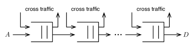
Figure 1: Tandem network model.

III Network Model in the Bit and SNR Domains

We consider a wireless $N$-node tandem network as shown in Fig. 1, where each node is modeled by a server with an infinite buffer. We are interested in the performance experienced by a (through) flow that traverses the entire network and may encounter cross traffic at each node. One can think of the cross traffic at a node as the aggregate of all traffic traversing the node that does not belong to the through flow. The service given to the through flow at a node is a random process, which is governed by the instantaneous channel capacity as well as the cross traffic at the node. We consider a fluid-flow traffic model where the flow is infinitely divisible. We will work in a discrete-time domain $\mathcal{T}=\{t_{i}:t_{i}=i\ \Delta t,i\in\mathds{Z}\}$, where $\mathds{Z}$ is the set of integers and $\Delta t$ is length of the time unit. Setting $\Delta t=1$ allows us to replace $t_{i}$ by $i$, which we interpret as the index of a time slot. We assume that the system is started with empty queues at time $t=0$.

Different nodes and different traffic flows will be distinguished by subscripts. The cumulative arrivals to, the service offered by, and the departures from the node are represented by random processes $A_{n}$, $S_{n}$, and $D_{n}$ that will be described more precisely below, with $A_{n}=D_{n-1}$ for $n=1,\dots,N-1$. We denote by $A=A_{1}$ and $D=D_{N}$ the arrivals to and the departures from the tandem network. Throughout, we assume that arrival and service processes satisfy stationary bounds.

III-A Traffic and Service in the Bit Domain

Consider for the moment a single node. Dropping subscripts, we write

$$A(\tau,t)=\sum_{i=\tau}^{t-1}a_{i}\,,\quad\text{and}\quad D(\tau,t)=\sum_{i=\tau}^{t-1}d_{i}\,,$$

for the cumulative arrivals and departures, respectively, at the node in the time interval $[\tau,t)$, where $a_{i}$ denotes the arrivals and $d_{i}$ the departures in the $i$-th time slot. Due to causality, we have $D(0,t)\leq A(0,t)$. The processes lie in the set ${\mathcal{F}}$ of non-negative bivariate functions $f(\tau,t)$ that are increasing in the second argument and vanish unless $0\leq\tau<t$. The backlog at time $t>0$ is given by

$$B(t)=A(0,t)-D(0,t)\ ,$$ (3)

and the delay at the node is given by

$$W(t)=\inf\left\{u\geq 0:A(0,t)\leq D(0,t+u)\right\}\ .$$ (4)

The service of the node in the time interval $[\tau,t)$ is given by a random process $S(\tau,t)$, such that Eq. (2) holds for every arrival process $A$ and the corresponding departure process $D$. This service description with bivariate functions is referred to as dynamic server. Initially defined for non-random service [6], dynamic servers have been extended to random processes in [5, 13].

The above model is a typical network-layer model. where traffic is measured in bits, and service is measured in bits per second. We thus refer to this model of arrivals, departures, and service as residing in a bit domain.

The network calculus exploits that networks which satisfy the input-output relation of Eq. (2) with equality can be viewed as linear systems in a $(\min,+)\,$dioid algebra [25]. In the ($\mathds{R}\cup\{+\infty\},\min,+$) dioid, the minimum and addition take the place of the standard addition and multiplication operations. The network calculus is based on the fact that $({\mathcal{F}},\min,\ast)$ is again a dioid [5]. Note that the min-plus convolution, which provides the second operation in the dioid, is not commutative in ${\mathcal{F}}$.

III-B Service Model of Wireless Channel

To compute a service model for a wireless channel, we assume that the channel state information is sampled at equal time intervals $\Delta t$. With $\Delta t=1$, let $\gamma_{i}$ denote the instantaneous signal-to-noise ratio observed at the receiver in the $i$-th sampling epoch. Then, $\gamma_{i}$ is a nonnegative random variable that has the probability distribution of the underlying fading model. We assume that the random variables $\gamma_{i}$ are independent and identically distributed. This assumption is justified when $\Delta t$ is longer than the channel coherence time. Otherwise, the assumption will give optimistic bounds. We emphasize that the network calculus in this paper applies to settings without independence, however, the derivation of performance bounds will proceed differently. Using Eq. (1), the instantaneous service offered by the channel in the $i$-th slot is given by $\log g(\gamma_{i})$. and the corresponding service process is given by

$$S(\tau,t)=\sum_{i=\tau}^{t-1}\log g(\gamma_{i})\,,$$ (5)

where we haven chosen units such that the constant in Eq. (1) takes the value $c=1$.

The service description in Eq. (5) requires us to work with the logarithm of fading distributions, which presents a non-trivial technical difficulty via the usual network calculus or queueing theory. On the other hand, observe that the exponential ${\cal S}(\tau,t)=e^{S(\tau,t)}$ is described more simply by

$${\cal S}(\tau,t)=\prod_{i=\tau}^{t-1}g(\gamma_{i})\ .$$ (6)

This motivates the development of a system model that allows us to exploit the more tractable service representation in Eq. (6). In this alternative model, arrivals, departures, and service reside in a different domain, where we can work directly with the distribution functions of the fading channel gain and the corresponding SNR at the receiver.

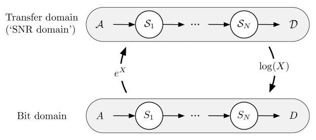
Figure 2: Transfer Domain of Network Model.

III-C Network Model in the SNR Domain

We now proceed by mapping the network model from Fig. 1 into a transfer domain, which we refer to as SNR domain. We will seek to derive performance bounds in the transfer domain, and then map the results to the bit domain to obtain network-layer bounds for backlog and delays. The relationship of the network models in bit domain and SNR domain is illustrated in Fig. 2.

In the previous subsection, we constructed the service process for a wireless link in the SNR domain in Eq. (6) as

$${\cal S}(\tau,t)=e^{S(\tau,t)}\,.$$

By analogy, we describe the arrivals and departures in the SNR domain by

$${\cal A}(\tau,t){\,{\buildrel\bigtriangleup\over{=}}\,}e^{A(\tau,t)}\,,\quad\text{and }\quad{\cal D}(\tau,t){\,{\buildrel\bigtriangleup\over{=}}\,}e^{D(\tau,t)}\,.$$

Throughout this paper, we use calligraphic upper-case letters to represent processes that characterize traffic or service as a function of the instantaneous SNR in the sense of Eq. (6). Due to the monotonicity of the exponential function, ${\cal D}(0,t)$ and ${\cal A}(0,t)$ are increasing in $t$, and satisfy the causality property ${\cal D}(0,t)\leq{\cal A}(0,t)$. The backlog process is accordingly described by

$${\cal B}(t){\,{\buildrel\bigtriangleup\over{=}}\,}e^{B(t)}={\cal A}(t)/{\cal D}(t)\,.$$

Since time is not affected by this transformation, the delay is given by

$${\mathcal{W}}(t){\,{\buildrel\bigtriangleup\over{=}}\,}W(t)=\inf\{u\geq 0:{\cal A}(t)\leq{\cal D}(t+u)\}\,.$$ (7)

To interpret these processes in the transfer domain, let $\gamma_{a,i}{\,{\buildrel\bigtriangleup\over{=}}\,}g^{-1}(e^{a_{i}})$ be the instantaneous channel SNR required to transmit $a_{i}$ in a single time slot, assuming transmission at the rate of the capacity limit. The arrival process in the SNR domain can then be expressed in terms of these variables as

$${\cal A}(\tau,t)=\prod_{i=\tau}^{t-1}g(\gamma_{a,i})\,.$$ (8)

Here, we are treating channel quality expressed in terms of the instantaneous SNR as a commodity. An arrival in a time unit represents a workload, where $\gamma_{a,i}$ expresses the amount of resources that will be consumed by the workload. The backlog can similarly be expressed in terms of the instantaneous SNR as

$${\cal B}(t)=\prod_{i=t}^{t+\tau_{B}-1}g(\gamma_{i})\ ,$$

with the interpretation that a node with backlog $B(t)$ at time $t$ requires full use of the channel capacity for $\tau_{B}$ time units to clear the backlog.

Most importantly, the concept of the dynamic server translates to the SNR domain. In a network system, the service process in the bit domain satisfies Eq. (2) if and only if the process ${\cal S}(\tau,t)=e^{S(\tau,t)}$ in the SNR domain satisfies

$${\cal D}(0,t)\geq\inf_{0\leq u\leq t}\{{\cal A}(0,u)\cdot{\cal S}(u,t)\}\ .$$ (9)

We refer to a network element that satisfies Eq. (9) for any sample path as dynamic SNR server. In this general setting, we not require that ${\cal S}$ takes the form in Eq. (6), in particular, ${\cal S}(\tau,t)$ does not be equal to ${\cal S}(\tau,u)\cdot{\cal S}(u,t)$.

Traffic aggregation in the SNR domain is expressed in terms of a product. When $M$ flows have arrivals at a node with arrival processes denoted by $A_{k},k=1,\ldots,M$, then the total arrival, $A_{\rm agg}$, are given for any $0\leq\tau\leq t$ by

$$A_{\rm agg}(\tau,t)=\sum_{k=1}^{M}A_{k}(\tau,t)\ .$$

If we let ${\cal A}_{j}$ and ${\cal A}_{\rm agg}$ denote the corresponding processes in the SNR domain, we see that

$${\cal A}_{\rm agg}(\tau,t)=\prod_{k=1}^{M}{\cal A}_{k}(\tau,t)\ .$$

With the above definitions, the usual network description by a $(\min,+)\,$dioid algebra in the bit domain can be expressed in the SNR domain by a dioid algebra on ${\mathcal{F}}$ where the second operator is a multiplication. This enables the development of the $(\min,\times)$ network calculus in Sec. IV. We observe that the exponential function defines a one-to-one correspondence between arrival and departure processes in the bit and SNR domains. The physical arrival, departure, service, and backlog processes can be recovered from their counterparts in the SNR domain by taking a logarithm (see Fig. 2).

IV Stochastic $(\min,\times)$  Network Calculus

This section contains our main contribution: an analytical framework for statistical end-to-end performance bounds for a network, where service is expressed in terms of fading distributions residing in the SNR domain.

By an SNR process we mean a bivariate process ${\mathcal{X}}(\tau,t)$ taking values in $\mathds{R}^{+}$ that is increasing in the second argument, with ${\mathcal{X}}(t,t)=1$ for all $t$. The space of SNR processes will be denoted by ${\mathcal{F}}^{+}$. For any pair of SNR processes ${\mathcal{X}}(\tau,t)$ and ${\mathcal{Y}}(\tau,t)$, set

$${\mathcal{X}}\otimes{\mathcal{Y}}(\tau,t){\,{\buildrel\bigtriangleup\over{=}}\,}\inf_{\tau\leq u\leq t}\big{\{}{\mathcal{X}}(\tau,u)\cdot{\mathcal{Y}}(u,t)\big{\}}\ ,$$ (10)

and

$${\mathcal{X}}\oslash{\mathcal{Y}}(\tau,t){\,{\buildrel\bigtriangleup\over{=}}\,}\sup_{u\leq\tau}\Big{\{}\frac{{\mathcal{X}}(u,t)}{{\mathcal{Y}}(u,\tau)}\Big{\}}\,.$$ (11)

We refer to ‘$\otimes$’ and ‘$\oslash$’ as the the $(\min,\times)$ convolution and $(\min,\times)$ deconvolution operators, respectively.

The arrival, departure, and service processes constructed in the previous section are SNR processes. With the $(\min,\times)$ convolution, we can express the defining property of a dynamic SNR server from Eq. (9) as

$$D(0,t)\geq A\otimes S(0,t)\$$ (12)

for every pair of SNR arrival and departure processes ${\cal A}(\tau,t)$ and ${\cal D}(\tau,t)$.

IV-A $(\min,\times)$ Dioid Algebras

We note that, in fact, for any system description in the bit domain by the ($\mathds{R}\cup\{+\infty\},\min,+$) and the (${{\mathcal{F}}},\min,\ast$) dioid algebras there exists a corresponding characterization in the SNR domain using ($\mathds{R}^{+}\cup\{+\infty\},\min,\times$) and (${{\mathcal{F}}^{+}},\min,\otimes$) dioids. The following argument confirm that the properties of a dioid are satisfied.

Lemma 1

$(\mathds{R}^{+}\cup\{+\infty\},\min,\times)$ is a dioid.

Proof:

We show that ($\mathds{R}^{+}\cup\{+\infty\},\min,\times$) satisfies the dioid axioms. For $a,b,c\in\{\mathds{R}^{+}\cup\{+\infty\}\}$:

1. Commutativity of $\min$: $\min(a,b)=\min(b,a)$.

2. Associativity of $\min$: $\min(\min(a,b),c)=\min(a,\min(b,c))$.

3. Idempotency of $\min$: $\min(a,a)=a$.

4. Associativity of $\times$: $(a\times b)\times c=a\times(b\times c)$.

5. Distributivity of $\times$: $\min(a,b)\times c=\min(a\times c,b\times c)$.

6. Existence of a null element: The null element is $+\infty$. since $\min(+\infty,a)=a$.

7. Absorption of the null element: $(+\infty)\times a=a\times(+\infty)=+\infty$.

8. Existence of a unity element: The unit of multiplication is 1, since $1\times a=a\times 1=a$.

∎

Lemma 2

$({\mathcal{F}}^{+},\min,\otimes)$ is a dioid.

Proof:

Given bivariate functions ${\mathcal{X}},{\mathcal{Y}},{\mathcal{Z}}\in{\mathcal{F}}^{+}$. Since the $\min$ operation is a pointwise minimum, properties of the $\min$ operation, that is, properties (1)–(3) from the proof of Lemma 1, follow from the $(\mathds{R}^{+}\cup\{+\infty\},\min,\times)$ dioid. For the remaining properties we have

• Associativity of $\otimes$:

  $$({\mathcal{X}}\otimes{\mathcal{Y}})\otimes{\mathcal{Z}}(\tau,t)$$

  $$=\inf_{\tau\leq u\leq t}\bigl{\{}\inf_{\tau\leq s\leq u}\bigl{\{}{\mathcal{X}}(\tau,s)\cdot{\mathcal{Y}}(s,u)\bigr{\}}\cdot{\mathcal{Z}}(u,t)\bigr{\}}$$

  $$=\inf_{\tau\leq s\leq u\leq t}\bigl{\{}{\mathcal{X}}(\tau,s)\cdot{\mathcal{Y}}(s,u)\cdot{\mathcal{Z}}(u,t)\bigr{\}}$$

  $$=\inf_{\tau\leq s\leq t}\bigl{\{}{\mathcal{X}}(\tau,s)\cdot\inf_{s\leq u\leq t}\bigl{\{}{\mathcal{Y}}(s,u)\cdot{\mathcal{Z}}(u,t)\bigr{\}}\bigr{\}}$$

  $$={\mathcal{X}}\otimes({\mathcal{Y}}\otimes{\mathcal{Z}})(\tau,t)\ .$$

• Distributivity of $\otimes$ over finite sums:

  $$\min({\mathcal{X}},{\mathcal{Y}})\otimes{\mathcal{Z}}(\tau,t)$$

  $$=\inf_{\tau\leq s\leq t}\bigl{\{}\min({\mathcal{X}},{\mathcal{Y}})(\tau,s)\cdot{\mathcal{Z}}(s,t)\bigr{\}}$$

  $$=\inf_{\tau\leq s\leq t}\bigl{\{}\min\bigl{(}{\mathcal{X}}(\tau,s)\cdot{\mathcal{Z}}(s,t),{\mathcal{Y}}(\tau,s)\cdot{\mathcal{Z}}(s,t)\bigr{)}\bigr{\}}$$

  $$=\min\left({\mathcal{X}}\otimes{\mathcal{Y}}(\tau,t),{\mathcal{Y}}\otimes{\mathcal{Z}}(\tau,t)\right)\,.$$

• Existence of a null element: The null element is $N(\tau,t)=+\infty$ for all values of $\tau$ and $t$.

• Absorption of the null element:

  $$N\otimes{\mathcal{X}}(\tau,t)=\inf_{\tau\leq u\leq t}\big{\{}(+\infty)\cdot{\mathcal{X}}(u,t)\big{\}}=+\infty\,.$$

  Note that functions in ${\mathcal{F}}^{+}$ are strictly positive by definition.

• Existence of a unity element: The unity element is $\Delta(\tau,t)$, where

  $$\Delta(\tau,t)=\begin{cases}1&\tau\geq t\,,\\ \infty&\tau<t\ .\end{cases}$$

  This gives

  $$\Delta\otimes{\mathcal{X}}(\tau,t) =\inf_{\tau\leq s\leq t}\bigl{\{}\Delta(\tau,s)\cdot{\mathcal{X}}(s,t)\bigr{\}}$$

  $$=\Delta(\tau,\tau)\cdot{\mathcal{X}}(\tau,t)$$

  $$={\mathcal{X}}(\tau,t)\,.$$

∎

IV-B Server Concatenation and Performance Bounds

The existing network calculus in the bit domain allows for the concatenation of tandem service elements using the $(\min,+)\,$ convolution (see page 1). As an immediate consequence, single node performance bounds are extended to a multi-hop setting. We now show establish the corresponding result in the $(\min,\times)$ network calculus. Specifically, the concatenation of dynamic SNR servers is again a dynamic SNR server. We will prove the result for a tandem network of two nodes, as shown in Fig. 3.

Lemma 3

Let ${\cal S}_{1}(\tau,t)$ and ${\cal S}_{2}(\tau,t)$ be two dynamic SNR servers in tandem as shown in Fig. 3. Then, the service offered by the tandem of nodes is given by the dynamic SNR server ${\cal S}_{\rm net}(\tau,t)$ with

$${\cal S}_{\rm net}(\tau,t)={\cal S}_{1}\otimes{\cal S}_{2}(\tau,t)\ .$$

Proof:

Using Eq. (9), the departure process ${\cal D}(0,t)$ can be written as

$${\cal D}(0,t) \geq \inf_{0\leq u\leq t}\{{\cal A}_{2}(0,u)\cdot{\cal S}_{2}(u,t)\}$$

$$\geq \inf_{0\leq u\leq t}\big{\{}\inf_{0\leq\tau\leq u}\{{\cal A}(0,\tau)\cdot{\cal S}_{1}(\tau,u)\}\cdot{\cal S}_{2}(u,t)\big{\}}$$

$$= \!\!\!\!\inf_{0\leq\tau\leq t}\big{\{}{\cal A}(0,\tau)\cdot\!\!\inf_{\tau\leq u\leq t}\{{\cal S}_{1}(\tau,u)\cdot{\cal S}_{2}(u,t)\}\big{\}}$$

$$= \!\!\!\!\inf_{0\leq\tau\leq t}\big{\{}{\cal A}(0,\tau)\cdot({\cal S}_{1}\otimes{\cal S}_{2})(\tau,t)\big{\}}\,.$$

∎

The extension to networks with more than two nodes follows by iteratively applying Lemma 3. Hence, the dynamic network SNR server with $N$ nodes in tandem is given by

$${\cal S}_{\rm net}(\tau,t)={\cal S}_{1}\otimes{\cal S}_{2}\otimes\cdots\otimes{\cal S}_{N}(\tau,t)\ .$$ (13)

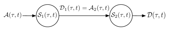
Figure 3: Tandem of dynamic SNR servers.

Performance bounds in the $(\min,\times)$ network calculus are computed with the $(\min,\times)$ deconvolution operator. This is analogous to role of the $(\min,+)\,$ deconvolution in the existing $(\min,+)\,$ network calculus. The bounds are expressed in the following lemma.

Lemma 4

Given a system with SNR arrival process ${\cal A}(\tau,t)$ and dynamic SNR server ${\cal S}(\tau,t)$.

• Output Burstiness. The SNR departure process is bounded by ${\cal D}(\tau,t)\leq{\cal A}\oslash{\cal S}(\tau,t)$.

• Backlog Bound. The SNR backlog process is bounded by ${\cal B}(t)\leq{\cal A}\oslash{\cal S}(t,t)$.

• Delay Bound. The delay process is bounded by ${\mathcal{W}}(t)\leq\inf\Big{\{}d\geq 0:{\cal A}\oslash{\cal S}(t+d,t)\leq 1\Big{\}}$.

Proof:

For the output bound, we fix $\tau$ and $t$ with $0\leq\tau\leq t$ and derive

$${\cal D}(\tau,t) = \frac{{\cal D}(0,t)}{{\cal D}(0,\tau)}\leq\frac{{\cal A}(0,t)}{{\cal D}(0,\tau)}$$

$$\leq \sup_{0\leq u\leq\tau}\Big{\{}\frac{{\cal A}(0,t)}{{\cal A}(0,u)\cdot{\cal S}(u,\tau)}\Big{\}}$$

$$= \sup_{0\leq u\leq\tau}\Big{\{}\frac{{\cal A}(u,t)}{{\cal S}(u,\tau)}\Big{\}}\,,$$

where we used the inequality ${\cal D}(0,\tau)\geq{\cal A}\otimes{\cal S}(0,\tau)\}$ in the second line.

For any fixed sample path, fix an arbitrary $t\geq 0$. The bound on the backlog is derived by

$${\cal B}(t) = \frac{{\cal A}(0,t)}{{\cal D}(0,t)}$$

$$\leq \sup_{0\leq u\leq t}\Big{\{}\frac{{\cal A}(0,t)}{{\cal A}(0,u)\cdot{\cal S}(u,t)}\Big{\}}$$

$$= \sup_{0\leq u\leq t}\Big{\{}\frac{{\cal A}(u,t)}{{\cal S}(u,t)}\Big{\}},$$

where we used ${\cal D}(0,t)\geq{\cal A}\otimes{\cal S}(0,t)\}$ in the second step.

Recall that the delay is invariant under the transform of domains, that is, ${\mathcal{W}}(t)=W(t)$. By definition of the delay in Eq. (7), a delay bound $w$ satisfies

$${\mathcal{W}}(t) = \inf\Big{\{}w\geq 0:\frac{{\cal A}(0,t)}{{\cal D}(0,t+w)}\leq 1\Big{\}}$$ (14)

$$\leq \!\!\!\inf\Big{\{}w\geq 0:\!\!\!\sup_{0\leq u\leq t}\Big{\{}\frac{{\cal A}(0,t)}{{\cal A}(0,u)\cdot{\cal S}(u,t+w)}\Big{\}}\leq 1\Big{\}}$$

$$= \inf\Big{\{}w\geq 0:\sup_{0\leq u\leq t}\Big{\{}\frac{{\cal A}(u,t)}{{\cal S}(u,t+w)}\Big{\}}\leq 1\Big{\}}.$$

where we used the inequality ${\cal D}(0,t+w)\geq{\cal A}\otimes{\cal S}(0,t+w)\}$ in the second line. ∎

With an algebraic description for network performance bounds in the SNR domain in hand, we now turn to the problem of computing the bounds.

IV-C The Mellin Transform in the SNR domain

The concise (and familiar) expressions from the previous section for the network service and performance bounds in the SNR domain hide the difficulty of computing the expressions. In fact, all expressions of the $(\min,\times)$ network calculus contain products or quotients of random variables. The Mellin transform [11] facilitates such computations, particularly when the arrival and service processes are independent.

The Mellin transform of a nonnegative random variable $X$ is defined by

$${\mathcal{M}}_{X}(s)=E[X^{s-1}]$$ (15)

for any complex number $s$ such that this expected value exists.

Among its many properties, we will exploit that the Mellin transform of a product of two independent random variables $X$ and $Y$ equals the product of their Mellin transforms,

$${\mathcal{M}}_{X\cdot Y}(s)={\mathcal{M}}_{X}(s)\cdot{\mathcal{M}}_{Y}(s).$$ (16)

Similarly, the Mellin transform of the quotient of independent random variables is given by

$${\mathcal{M}}_{X/Y}(s)={\mathcal{M}}_{X}(s)\cdot{\mathcal{M}}_{Y}(2-s).$$ (17)

We will evaluate the Mellin transform only for $s\in\mathds{R}$, where it is always well-defined (though it may take the value $+\infty$). When $s>1$, the Mellin transform is order-preserving, i.e., for any pair of random variables $X,Y$ with ${Pr}(X>Y)=0$ we have ${\mathcal{M}}_{X}(s)\leq{\mathcal{M}}_{Y}(s)$ for all $s$. When $s<1$, the order is reversed. Hence bounds on the distribution of a random variable $X$ generally imply bounds on its Mellin transform.

A more subtle question is how to obtain bounds on the distribution of a random variable from its Mellin transform. Here, the complex inversion formula is not helpful. Instead, we will use the moment bounds

$${Pr}(X\geq a) \leq a^{-s}{\mathcal{M}}_{X}(1+s)$$ (18)

for all $a>0$ and $s>0$. For bivariate random processes ${\mathcal{X}}(\tau,t)$, we will write ${\mathcal{M}}_{{\mathcal{X}}}(s,\tau,t){\,{\buildrel\bigtriangleup\over{=}}\,}{\mathcal{M}}_{{\mathcal{X}}(\tau,t)}(s)$.

In our calculus, we work with the Mellin transform of $(\min,\times)$ convolutions and deconvolutions, which not only involves products and quotients, but also requires to compute infimums and supremums. The computation of the exact Mellin transform for these operations is generally not feasible. We therefore resort to bounds, as specified in the next lemma.

Lemma 5

Let ${\mathcal{X}}(\tau,t)$ and ${\mathcal{Y}}(\tau,t)$ be two independent nonnegative bivariate random processes. For $s<1$, the Mellin transform of the $(\min,\times)$ convolution ${\mathcal{X}}\otimes{\mathcal{Y}}(\tau,t)$ is bounded by

$${\mathcal{M}}_{{\mathcal{X}}\otimes{\mathcal{Y}}}(s,\tau,t)\leq\sum_{u=\tau}^{t}{\mathcal{M}}_{{\mathcal{X}}}(s,\tau,u)\cdot{\mathcal{M}}_{\mathcal{Y}}(s,u,t)\,.$$ (19)

For $s>1$, the Mellin transform of the $(\min,\times)$ deconvolution ${\mathcal{X}}\oslash{\mathcal{Y}}(\tau,t)$ is bounded by

$${\mathcal{M}}_{{\mathcal{X}}\oslash{\mathcal{Y}}}(s,\tau,t)\leq\sum_{u=0}^{\tau}{{\mathcal{M}}_{{\mathcal{X}}}(s,u,t)}\cdot{{\mathcal{M}}_{{\mathcal{Y}}}(2\!-\!s,u,\tau)}\,.$$ (20)

Proof:

Note that the function $f(z)=z^{s-1}$ is increasing for $s>1$ and decreasing for $s<1$. For $s<1$, the convolution is estimated by

$${\mathcal{M}}_{{\mathcal{X}}\otimes{\mathcal{Y}}}(s,\tau,t) =E\Bigl{[}\Bigl{(}\ \inf_{\tau\leq u\leq t}\{{\mathcal{X}}(\tau,u)\cdot{\mathcal{Y}}(u,t)\}\Bigr{)}^{s-1}\Bigr{]}$$

$$=E\Bigl{[}\ \sup_{\tau\leq u\leq t}\{({\mathcal{X}}(\tau,u))^{s-1}\cdot({\mathcal{Y}}(u,t))^{s-1}\}\Bigr{]}$$

$$\leq\sum_{u=\tau}^{t}E\big{[}({\mathcal{X}}(\tau,u))^{s-1}\big{]}\cdot E\big{[}({\mathcal{Y}}(u,t))^{s-1}\big{]}\,.$$

In the last line, we have used the non-negativity of ${\mathcal{X}}$ and ${\mathcal{Y}}$ to replace the supremum with a sum, and their independence to evaluate the expectation of the products. Eq. (19) follows by inserting the definition of the Mellin transform. The deconvolution is similarly estimated for $s>1$ by

$${\mathcal{M}}_{{\mathcal{X}}\oslash{\mathcal{Y}}}(s,\tau,t) =E\Bigl{[}\Bigl{(}\ \sup_{u\leq\tau}\bigl{\{}{\mathcal{X}}(u,t)/{\mathcal{Y}}(u,\tau)\bigr{\}}\bigr{)}^{s-1}\Bigr{]}$$

$$=E\Bigl{[}\ \sup_{0\leq u\leq\tau}\bigl{\{}\bigl{(}{\mathcal{X}}(u,t)\bigr{)}^{s-1}\cdot\bigl{(}{\mathcal{Y}}(u,\tau)\bigr{)}^{1-s}\bigr{\}}\Bigr{]}$$

$$\leq\sum_{u=0}^{\tau}E\bigl{[}\bigl{(}{\mathcal{X}}(u,t)\bigr{)}^{s-1}\bigr{]}\cdot E\bigl{[}\bigl{(}{\mathcal{Y}}(u,\tau)\bigr{)}^{1-s}\bigr{]}\,,$$

and Eq. (20) follows from the definition of the Mellin transform. ∎

As an application of Lemmas 3 and 5, we compute a bound on the Mellin transform of the service process for a cascade of fading channels. We also make the idealizing assumption that the channels are independent.

Corollary 1

Consider a cascade of $N$ independent, identically distributed fading channels, where the service process for each channel is given by Eq. (6), with i.i.d. random variables $\gamma_{i}$. Let ${\cal S}_{\rm net}(\tau,t)$ denote the SNR service process for the entire cascade. Then, the Mellin transform for this process satisfies

$${\mathcal{M}}_{{\cal S}_{\rm net}}(s,\tau,t)\leq\binom{N-1+t-\tau}{t-\tau}\cdot\bigl{(}{\mathcal{M}}_{g(\gamma)}(s)\bigr{)}^{t-\tau}$$

for all $s<1$.

Proof:

We use the server concatenation formula in Eq. (13) to represent the service of the cascade as ${\cal S}_{\rm net}(\tau,t)={\cal S}_{1}\otimes{\cal S}_{2}\otimes\dots\otimes{\cal S}_{N}(\tau,t)$. By Lemma 5, its Mellin transform satisfies for $s<1$

$${\mathcal{M}}_{{\cal S}_{\rm net}}(s,\tau,t) \leq\sum_{u_{1}\dots u_{N-1}}\prod_{n=1}^{N}M_{\cal S}(s,u_{n-1},u_{n})\,,$$ (21)

where the sum runs over all sequences $u_{0}\leq u_{1}\leq\dots\leq u_{N}$ with $u_{0}=\tau$ and $u_{N}=t$. The assumptions on the service processes of the individual channels imply that each product evaluates to the same function

$$\prod_{n=1}^{N}M_{\cal S}(s,u_{n-1},u_{n}) =\prod_{n=1}^{N}\bigl{(}{\mathcal{M}}_{g(\gamma)}(s)\bigr{)}^{u_{n}-u_{n-1}}$$

$$=\bigl{(}{\mathcal{M}}_{g(\gamma)}(s)\bigr{)}^{t-\tau}\,,$$

where $\gamma$ is a random variable that has the same distribution as the $\gamma_{i}$. Since the number of summands in Eq. (21) is given by $\binom{N-1+t-\tau}{t-\tau}$, the claim follows. ∎

IV-D Performance Bounds for the Bit Domain

We next obtain network-level performance bounds for the bit domain. This involves a transformation from the SNR domain to the bit domain via the relationship in Fig. 2, which provides the translation of the abstract metrics ${\cal D}$ and ${\cal B}$ into processes $D$ and $B$, which, along with $W$, are concrete measures for traffic burstiness, buffer requirements, and delay.

Theorem 1

Given a system where arrivals are described by a bivariate process $A(\tau,t)$, and the available service is given by a dynamic server $S(\tau,t)$. Let ${\cal A}(\tau,t)$ and ${\cal S}(\tau,t)$ be the corresponding SNR processes. Fix $\varepsilon>0$ and define, for $s>0$,

$${\mathsf{M}}(s,\tau,t)=\sum_{u=0}^{\min(\tau,t)}{\mathcal{M}}_{{\cal A}}(1+s,u,t)\cdot{\mathcal{M}}_{{\cal S}}(1-s,u,\tau)\,.$$

Then, we have the following probabilistic performance bounds.

$\bullet$ Output Burstiness: ${Pr}\bigl{(}D(\tau,t)>d^{\varepsilon}\bigr{)}\leq\varepsilon$, where

$$d^{\varepsilon}(\tau,t)=\inf_{s>0}\Big{\{}\frac{1}{s}\bigl{(}\log{\mathsf{M}}(s,\tau,t)-\log\varepsilon\bigr{)}\Big{\}}\,;$$

$\bullet$ Backlog: ${Pr}\bigl{(}B(t)>b^{\varepsilon}\bigr{)}\leq\varepsilon$, where

$$b^{\varepsilon}=\inf_{s>0}\Big{\{}\frac{1}{s}\bigl{(}\log{\mathsf{M}}(s,t,t)-\log\varepsilon\bigr{)}\Big{\}}\,;$$

$\bullet$ Delay: ${Pr}\bigl{(}W(t)>w^{\varepsilon}\bigr{)}\leq\varepsilon$, where $w^{\varepsilon}$ is the smallest number satisfying

$$\inf_{s>0}\Big{\{}{\mathsf{M}}(s,t+w^{\varepsilon},t)\Big{\}}\leq\varepsilon\,.$$

Proof:

For the bound on the distribution of the output burstiness, we start from the inequality ${\cal D}(\tau,t)\leq{\cal A}\otimes{\cal S}(\tau,t)$. It follows from the moment bound and Lemma 5 that, for any choice of $d>0$ and all $s>0$

$${Pr}(D(\tau,t)>d) ={Pr}({\cal D}(t)>e^{d})$$

$$\leq{Pr}({\cal A}\oslash{\cal S}(\tau,t)>e^{d})$$

$$\leq(e^{d})^{-s}{\mathcal{M}}_{{\cal A}\oslash{\cal S}}(1+s,\tau,t)$$

$$=e^{-sd}{\mathsf{M}}(s,\tau,t)\,.$$

To obtain the claim, we set the right hand side equal to $\varepsilon$, solve for $d$, and optimize over the value of $s>0$ to obtain $d^{\varepsilon}(\tau,t)$. The proof of the backlog bound proceeds in the same way, starting from the inequality ${\cal B}(t)\leq{\cal A}(0,t)/{\cal D}(0,t)$.

The delay bound is slightly more subtle. Fix $t\geq 0$. Using Lemma 4 and the moment bound with $a=1$, we obtain that

$${Pr}({\mathcal{W}}(t)>w) \leq{Pr}({\cal A}\oslash{\cal S}(t+w,t)>1)$$

$$\leq{\mathcal{M}}_{A\oslash{\cal S}}(s+1,t+w,t)\,$$

for every $s>0$. By Lemma 5, the Mellin transform ${\mathcal{M}}_{A\oslash{\cal S}}(s+1,t+w,t)$ satisfies a bound that agrees with the function ${\mathsf{M}}(s,t+w,t)$, except that the upper limit in the summation that defines ${\mathsf{M}}(s,t+w,t)$ would have to be replaced by $\tau=t+w$. To obtain a sharper estimate, we use instead Eq. (14) from the proof of Lemma 4. The resulting bound is that

$${\mathcal{Z}}(t){\,{\buildrel\bigtriangleup\over{=}}\,}\sup_{0\leq u\leq t}\Bigl{\{}\frac{{\cal A}(u,t)}{{\cal S}(u,t+w)}\Bigr{\}}$$

satisfies

$${Pr}({\mathcal{W}}(t)>w) \leq{Pr}({\mathcal{Z}}(t)>1)$$

$$\leq{\mathcal{M}}_{{\mathcal{Z}}(t)}(s+1)$$

$$\leq{\mathsf{M}}(s,t+w,t)\,,$$ (22)

where we have used that the supremum in the definition of ${\mathcal{Z}}$ extends only up to $u=t$, and then repeated the proof Eq. (20). The claim follows by optimizing over $s$. ∎

Corresponding bounds as in Theorem 1 can be obtained using the $(\min,+)\,$algebra and the network calculus with moment-generating functions [13]. The significance of Theorem 1 is that it permits the application of the the network calculus, where traffic is characterized in the bit domain, and service is naturally expressed in the SNR domain. This will become evident in the next section, where the Theorem gives us concise bounds for delays and backlog of multi-hop networks with Rayleigh fading channels.

V Network Performance of Rayleigh Channels

We now apply the techniques developed in the two previous sections to a network of Rayleigh channels. Consider the dynamic SNR server description for a Rayleigh fading channel, as constructed in Sec. III.B. We use Eq. (6), with the function $g(\gamma)$ given by

$$g(\gamma)=1+\gamma=1+\bar{\gamma}|h|^{2},$$ (23)

where $\bar{\gamma}$ is the average SNR of the channel and $|h|$ is the fading gain. For Rayleigh fading, $|h|$ is a Rayleigh random variable with probability density $f(x)=2xe^{-x^{2}}$. In a physical system, $\bar{\gamma}=\bar{P}_{r}/\sigma^{2}$, where $\bar{P}_{r}$ and $\sigma^{2}$ are the received signal power and the (additive white Gaussian) noise power at the receiver, respectively. Then, $|h|^{2}$ is exponentially distributed, and the Mellin transform of $g(\gamma)$ is given by

$${\mathcal{M}}_{g(\gamma)}(s)=e^{1/\bar{\gamma}}\bar{\gamma}^{s-1}\Gamma(s,\bar{\gamma}^{-1})\,,$$

where $\Gamma(s,y)=\int_{y}^{\infty}x^{s-1}e^{-x}\,dx$ is the upper incomplete Gamma function. Using the assumption that the $\gamma_{i}$ are independent and identically distributed, we obtain for the Mellin transform of the dynamic server

$${\mathcal{M}}_{{\cal S}}(s,\tau,t)=\Bigl{(}e^{1/{\bar{\gamma}}}\bar{\gamma}^{s-1}\Gamma(s,\bar{\gamma}^{-1})\Bigr{)}^{t-\tau}.$$ (24)

For the arrival process, we use a characterization due to Chang [5], where the moment-generating function of the cumulative arrival process in the bit domain is bounded by

$$\frac{1}{s}\log E[e^{sA(\tau,t)}]\leq\rho(s)\cdot(t-\tau)+\sigma(s)$$

for some $s>0$. In general, $\rho(s)$ and $\sigma(s)$ are nonnegative increasing functions of $s$ that may become infinite when $s$ is large. This traffic class, referred to as $(\sigma(s),\rho(s))$ bounded arrivals, is broad enough to include Markov-modulated arrival processes. The corresponding class of SNR arrival processes is defined by the condition that

$${\mathcal{M}}_{{\cal A}}(s,\tau,t)\leq e^{(s-1)\cdot(\rho(s-1)\cdot(t-\tau)+\sigma(s-1))}\$$ (25)

for some $s>1$.

V-A Performance Bounds of Rayleigh Fading Channels

We consider the transmission of $(\sigma(s),\rho(s))$ bounded arrivals on a Rayleigh fading channel. To obtain single-hop performance bounds, we apply Theorem 1 with the expressions for the Mellin transforms for the SNR service and arrival processes from Eqs. (24) and (25). For the function ${\mathsf{M}}(s,\tau,t)$ from the statement of the theorem, we compute

$${\mathsf{M}}(s,\tau,t) \leq\ e^{s(\rho(s)(t-\tau)+\sigma(s))}\sum_{u=[\tau-t]_{+}}^{\infty}\big{(}\underbrace{e^{s\rho(s)}e^{1/\bar{\gamma}}\bar{\gamma}^{-s}\Gamma(1-s,\bar{\gamma}^{-1})}_{{\,{\buildrel\bigtriangleup\over{=}}\,}V(s)}\big{)}^{u}\,,$$

where $[\tau-t]_{+}$ is the maximum of $\tau-t$ and $0$. The sum converges when $V(s)<1$, which can be interpreted as a stability condition. Inserting the result into Theorem 1, we obtain for the output burstiness the probabilistic bound

$$d^{\varepsilon}_{\rm net}(\tau,t) =\inf_{s>0}\Bigl{\{}\rho(s)(t-\tau)+\sigma(s)-\frac{1}{s}\bigl{(}\log(1\!-\!V(s))+\log\varepsilon\bigr{)}\Bigr{\}}\,.$$

The backlog bound is obtained by setting $\tau=t$,

$$b^{\varepsilon}=\inf_{s>0}\left\{\sigma(s)-\frac{1}{s}\bigl{(}\log(1-V(s))+\log\varepsilon\bigr{)}\right\}\,.$$

The delay bound is the smallest number $w^{\varepsilon}$ such that

$$\inf_{s>0}\Bigl{\{}\frac{e^{s\cdot(-\rho(s)w^{\varepsilon}+\sigma(s))}}{1-V(s)}\cdot(V(s))^{w^{\varepsilon}}\Bigr{\}}\leq\varepsilon\,.$$

We also derive end-to-end bounds for a cascade of $N$ Rayleigh channels with $(\sigma(s),\rho(s))$ bounded arrivals, using the same parameters as before. Let ${\cal S}_{\rm net}(\tau,t)$ be the service process for the entire cascade. By Corollary 1, its Mellin transform satisfies for $0\leq\tau\leq t$

$${\mathcal{M}}_{{\cal S}_{\rm net}}(s,\tau,t)\leq\binom{N-1+t-\tau}{t-\tau}\cdot\Bigl{(}e^{1/{\bar{\gamma}}}\bar{\gamma}^{s-1}\Gamma(s,\bar{\gamma}^{-1})\Bigr{)}^{t-\tau}\!.$$

We will use again Theorem 1. For $0\leq\tau\leq t$, we compute

$${\mathsf{M}}_{\rm net}(s,\tau,t) \leq\ \frac{e^{s\cdot(\rho(s)(t-\tau)+\sigma(s))}}{(1-V(s))^{N}}\,,$$

where $V(s)$ is as defined above, and where we applied the combinatorial identity

$$\sum_{u=0}^{\infty}x^{u}\binom{N-1+u}{u}=\frac{1}{(1-x)^{N}}\ ,$$ (26)

for any $N>1$ and for $0<x<1$. Inserting ${\mathsf{M}}_{\rm net}(s,\tau,t)$ into Theorem 1 gives for the end-to-end output bound, denoted by $d^{\varepsilon}_{\rm net}(\tau,t)$, the value

$$d^{\varepsilon}_{\rm net}(\tau,t) =\inf_{s>0}\Bigl{\{}\rho(s)(t-\tau)+\sigma(s)-\frac{1}{s}\bigl{(}N\log(1\!-\!V(s))+\log\varepsilon\bigr{)}\Bigr{\}}\,.$$

Note that for $N=1$, this bound agrees with the previous bound for a single node. In the same way, we derive the probabilistic backlog bound

$$b^{\varepsilon}_{\rm net} =\inf_{s>0}\left\{\sigma(s)-\frac{1}{s}\bigl{(}N\log(1-V(s))+\log\varepsilon\bigr{)}\right\}\,.$$ (27)

For the delay bound, we estimate for $w\geq 0$

$${\mathsf{M}}_{\rm net}(s,r+w,t) \leq\ e^{-s(\rho(s)w+\sigma(s))}\sum_{u=w}^{\infty}\binom{N-1+u}{u}(V(s))^{u}$$

$$\leq\ \frac{e^{s(-\rho(s)w+\sigma(s))}}{(1-V(s))^{N}}\cdot\min\left\{1,(V(s))^{w}w^{N-1}\right\}\,.$$ (28)

Here, the first term in the minimum is obtained by extending the summation down to $u=0$, and the second term results from the inequality

$$\binom{N-1+u}{u}\leq w^{N-1}\cdot\binom{N-1+u-w}{u-w}$$

for $u\geq w$. In both cases, the resulting sum can be evaluated with Eq. (26). The delay bound $w^{\varepsilon}$ is determined according to Theorem 1 by setting the right hand side of Eq. (28) equal to $\varepsilon$, solving for $w$, and minimizing over $s$. Because of the complexity of the bound in Eq. (28), the last two steps can only be performed numerically.

It is apparent that the complexity of computing end-to-end bounds is no different than bounds for a single channel. More importantly, observe that the end-to-end bounds scale linearly in the number of nodes $N$. Relaxing the strong independence assumptions on the channel properties would give different scaling properties.

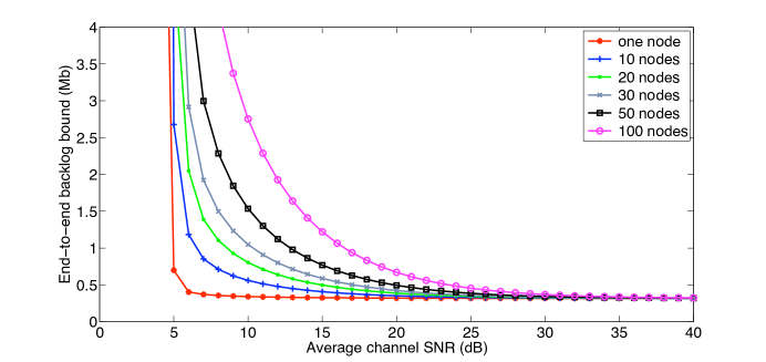
Figure 4: End-to-end backlog bound ($b^{\varepsilon}_{\rm net}$) vs. average channel SNR ($\bar{\gamma}$) for multihop Rayleigh fading channels with $\varepsilon=10^{-4}$, $(\sigma(s),\rho(s))$ bounded traffic with $\sigma(s)=50$ kb and $\rho(s)=30$ kbps, and $W=20$ kHz.

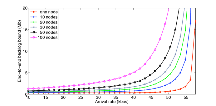
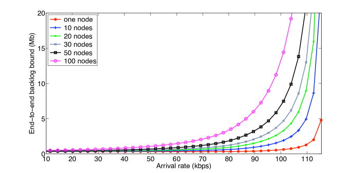
Figure 5: End-to-end backlog bound ($b_{net}^{\varepsilon}$) vs. arrival rate ($\rho(s)$) for multi-hop Rayleigh fading channels with $\varepsilon=10^{-4}$, $(\sigma(s),\rho(s))$ bounded traffic with $\sigma(s)=50$ kb and $\bar{\gamma}=10$ dB, and $W=20$ kHz.

Figure 6: End-to-end backlog bound ($b^{\varepsilon}_{\rm net}$) vs. arrival rate ($\rho(s)$) for multi-hop Rayleigh fading channels with $\varepsilon=10^{-4}$, $(\sigma(s),\rho(s))$ bounded traffic with $\sigma(s)=50$ kb, $\bar{\gamma}=20$ dB, and $W=20$ kHz.

V-B Numerical Examples

We next present numerical results, where we assume Rayleigh channels with a transmission bandwidth of $W=20$ kHz. For traffic, we use $(\sigma(s),\rho(s))$ bounded arrivals with default values $\sigma(s)\equiv 50$ kb and $\rho(s)\equiv 30$ kbps, i.e., the bounds on rate and bursts are deterministic. Hence, the source of randomness in the examples results only from randomness of the channels. We use a violation probability of $\varepsilon=10^{-4}$.

In Fig. 4 we show the end-to-end backlog for cascades of $N$ Rayleigh channels, as a function of the average SNR of each channel. Even though the backlog bounds increase only linearly in the number of nodes, the per-node requirements – at least for the last node of the cascade – must satisfy the end-to-end bounds, since it cannot be assumed that backlog is equally distributed across the nodes. When the SNR of the nodes is sufficiently high, the backlog remains low even for a large number of hops. We observe that the channel becomes saturated for $\bar{\gamma}=5$ dB. When the number of channels is small, the backlog increases sharply in the vicinity of $\bar{\gamma}=5$, but remains low everywhere else.

In Figs. 6 and 6 we present, for values of the average SNR of $\bar{\gamma}=10$ dB (Fig. 6) and $\bar{\gamma}=20$ dB (Fig. 6), how the end-to-end backlog increases as a function of the transmission rate, for different network sizes. We observe that the maximum achievable rate that does not result in a ‘blow-up’ of the backlog decreases as the number of nodes is increased. We observe that the blow-up occurs earlier when the channel has a lower SNR.

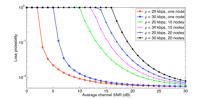
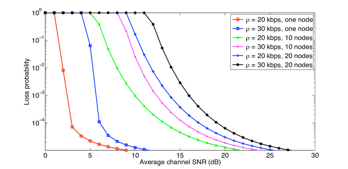
Figure 7: Loss probability ($\varepsilon(b)$) vs. average channel SNR ($\bar{\gamma}$) for multi-hop Rayleigh fading channels for $N=1,10$ and $20$, with buffer size $200$ kb, $(\sigma(s),\rho(s))$ bounded traffic with $\sigma(s)=50$ kb and $\rho(s)=20$ or $30$ kbps, and $W=20$ kHz.

Figure 8: Loss probability ($\varepsilon(b)$) vs. average channel SNR ($\bar{\gamma}$) for multi-hop Rayleigh fading channels for $N=1,10$ and $20$ with buffer size $400$ kb, $(\sigma(s),\rho(s))$ bounded traffic with $\sigma(s)=50$ kb and $\rho(s)=20$ or $30$ kbps, and $W=20$ kHz.

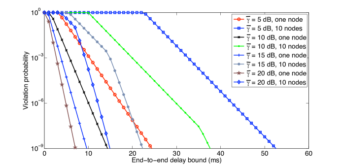
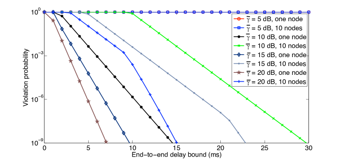
Figure 9: Delay bound violation probability ($\varepsilon(w)$) vs. end-to-end delays for multi-hop Rayleigh fading channels for $N=1,10$, $\bar{\gamma}=5,10,15,20$ dB, $(\sigma(s),\rho(s))$ bounded traffic with $\sigma(s)=50$ kb and $\rho(s)=20$ kbps and $W=20$ kHz.

Figure 10: Delay bound violation probability ($\varepsilon(w)$) vs. end-to-end delay bound for multi-hop Rayleigh fading channels for $N=1,10$, $\bar{\gamma}=5,10,15,20$ dB, $(\sigma(s),\rho(s))$ bounded traffic with $\sigma(s)=50$ kb and $\rho(s)=30$ kbps and $W=20$ kHz.

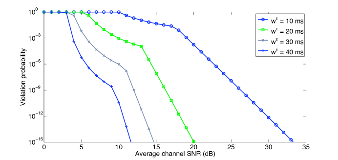
Figure 11: Delay bound violation probability ($\varepsilon(w)$) vs. average channel SNR ($\bar{\gamma}$) for multi-hop Rayleigh fading channels for $N=10$, $w^{\varepsilon}=10,20,30,40$ ms, $(\sigma(s),\rho(s))$ bounded traffic with $\sigma(s)=~{}50$ kb and $\rho(s)=20$ kbps and $W=20$ kHz.

Suppose that buffer sizes are set to satisfy the end-to-end backlog. For a fixed buffer size $b_{\rm max}$, we can then use the probability ${Pr}(B_{\rm net}(t)>b_{\rm max})$ as an estimate of the probability of dropped traffic, and refer to it as the loss probability. In Figs. 8 and 8, we depict the loss probability as a function of the average channel SNR, for values of $b_{\rm max}=200$ kb (Fig. 8) and $b_{\rm max}=400$ kb (Fig. 8), for traffic with a rate of $\rho(s)=20$ and $30$ kbps, and for $N=1,10$, and $20$ nodes. The figure shows the minimum SNR needed to support a given loss probability is very sensitive to the number of network nodes.

In Figs. 10 and 10 we show the violation probability for given end-to-end delay bounds, where we compare the delays at a single node ($N=1$) with a multi-hop network ($N=10$) for different average channel SNR values, where we use Eqs. (22) and (28). The traffic parameters are $\sigma(s)=50$ kb for the burst, and $\rho(s)=20$ kbps (in Fig. 10) $\rho(s)=30$ kbps (in Fig. 10). The figures illustrates that at sufficiently high SNR values, low delays are achieved even when traffic traverses 10 links. When the SNR is decreased, we can observe how the delay performance deteriorates in the multi-hop scenario. Note that the curves for the violation probability are essentially piecewise linear with two segments. This is caused by the different exponential decay rates, which follows from Eq. (28). Depending on where in the equation the minimum occurs, we obtain a faster or slower decay.

Next we investigate how the delay violation probability for given end-to-end delay bounds is impacted by the SNR of the channel. We consider a network with $N=10$ nodes, with the same parameters as before. The traffic parameters are $\sigma(s)=50$ kb and $\rho(s)=20$ kbps. We consider end-to-end delay bounds of $w^{\varepsilon}=10,20,30,40$ ms. Figs. 11 presents the results. An interesting observation is that the SNR required to support a given violation probability for a short delay bound $w^{\varepsilon}=10$ ms, the SNR requirement increase fast for low violation probabilities. Delay bounds $w^{\varepsilon}=20$ ms and higher can be supported with low violation probabilities even when the average SNR is small.

The graphs presented here can be used in the planning of a multi-hop wireless network where predefined QoS bounds are desired for a given transmission rate. Since the average SNR depends largely on the path loss, which, in turn, is a function of the transmission radius, the graphs could help with determining the maximum distance between nodes to support a desired transmission rate and QoS.

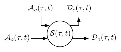
Figure 12: Single Fading Channel with Cross Traffic.

VI Fading Channels With Cross Traffic

Consider a scenario in Fig. 12 where a through flow arriving to a fading channel shares the available bandwidth with other flows. We will refer to the traffic from these other flows as cross traffic. We use ${\cal A}_{o}(\tau,t)$ and ${\cal A}_{c}(\tau,t)$ to denote the SNR arrival processes of the through flow and the cross traffic, respectively, and let ${\cal D}_{o}(\tau,t)$ and ${\cal D}_{c}(\tau,t)$ denote the corresponding departure processes. In the SNR domain, cross traffic can be viewed as reducing the channel capacity of the through flow by generating interference.

The following lemma states that, in the SNR domain, the service available to a through flow that experiences cross traffic at a channel can be expressed by a dynamic SNR server.

Lemma 6

Consider a channel with a through flow and cross traffic as shown in Fig. 12. Assume that the channel provides a dynamic SNR server to the aggregate of through flow and cross traffic, with service process ${\cal S}(\tau,t)$, i.e,

$${\cal D}_{o}(0,t)\cdot{\cal D}_{c}(0,t)\geq({\cal A}_{o}\cdot{\cal A}_{c})\otimes{\cal S}(0,t)\,.$$

Then

$${\cal S}_{o}(\tau,t)=\frac{{\cal S}(\tau,t)}{{\cal A}_{c}(\tau,t)}$$

is a dynamic SNR server satisfying for all $t\geq 0$ that

$${\cal D}_{o}(0,t)\geq{\cal A}_{o}\otimes{\cal S}_{o}(0,t)\,.$$ (29)

If, moreover, the service to the cross flows satisfies the upper bound ${\cal D}_{c}(0,t)\leq{\cal A}_{c}\otimes{\cal S}(0,t)$, then

$${\cal D}_{o}(0,t)\geq{\cal A}_{o}\otimes\max\{1,{\cal S}_{o}\}(0,t)\,.$$ (30)

Proof:

For any a sample path, and any $t\geq 0$, we have

$${\cal D}_{o}(0,t)\cdot{\cal D}_{c}(0,t)\geq\inf_{0\leq\tau\leq t}\{({\cal A}_{o}(0,\tau)\cdot{\cal A}_{c}(0,\tau))\cdot{\cal S}(\tau,t)\}\ .$$

Let $\tau^{*}$ be the point where the infimum is assumed. Dividing by ${\cal D}_{c}(\tau,t)$, we obtain

$${\cal D}_{o}(0,t) \geq\frac{({\cal A}_{0}\cdot{\cal A}_{c})\otimes{\cal S}(0,t)}{{\cal D}_{c}(0,t)}$$

$$\geq\frac{{\cal A}_{o}(0,\tau^{*})\cdot{\cal A}_{c}(0,\tau^{*})\cdot{\cal S}(\tau^{*},t)}{{\cal D}_{c}(0,t)}\Big{\}}$$

$$\geq\Big{\{}{\cal A}_{o}(0,\tau^{*})\cdot\frac{{\cal S}(\tau^{*},t)}{{\cal A}_{c}(\tau^{*},t)}\Big{\}}\,,$$

where we used that ${\cal D}_{c}(0,t)\leq{\cal A}_{c}(0,t)$ by causality. This the first claim in Eq. (29). To see the second claim, assume that ${\cal D}_{c}(0,t)\leq{\cal A}_{c}\otimes{\cal S}(0,t)$. Then ${\cal D}_{c}(0,t)\leq{\cal A}_{c}(0,\tau^{*})\cdot{\cal S}(\tau^{*},t)$, and therefore

$${\cal D}_{o}(0,t) \geq\frac{{\cal A}_{o}(0,\tau^{*})\cdot{\cal A}_{c}(0,\tau^{*})\cdot{\cal S}(\tau^{*},t)}{A_{c}(0,\tau^{*})\cdot{\cal S}(\tau^{*},t)}$$

$$={\cal A}_{0}(\tau^{*},t)\,.$$

Combining this with the first part of the proof, we obtain

$${\cal D}_{0}(0,t)\geq{\cal A}_{0}(0,\tau^{*})\cdot\max\{1,{\cal S}_{o}(\tau^{*},t)\}\,,$$

proving the second claim. ∎

Note that ${\cal S}_{o}(\tau,t)$ need not be monotone in $t$, i.e., it may not lie in ${\mathcal{F}}^{+}$.

VI-A Performance Bounds With Cross Traffic

We next estimate the service process available to the through flow across a cascade of channels. Assuming that ${\cal A}_{c}$ and ${\cal S}$ are independent, we obtain for the Mellin transform of the service process at a single node

$${\mathcal{M}}_{{\cal S}_{o}}(s,\tau,t) ={\mathcal{M}}_{{{\cal S}}/{{\cal A}_{c}}}(s,\tau,t)$$

$$={\mathcal{M}}_{{\cal S}}(s,\tau,t)\cdot{\mathcal{M}}_{{\cal A}_{c}}(2-s,\tau,t)\,.$$ (31)

These service descriptions may be convolved, using Lemmas 3 and 5 to obtain a bound for the Mellin transform of the service provided by a cascade of fading channels to a flow that experiences cross traffic at each node.

Corollary 2

Consider a network as in Fig. 1, where a through flow experiences cross traffic at each fading channel. Let the SNR service process at each channel be given by Eq. (6). Assume that the arrival process of the cross traffic satisfies Eq. (25) with parameters $(\sigma_{c}(s),\rho_{c}(s))$. Assume that arrivals from through flow and cross traffic, as well as the service processes at each channel are independent. Then, the service provided by the network to the through flow satisfies ${\cal D}_{o}(0,t)\geq{\cal A}_{o}\otimes{\cal S}_{o,\rm net}(0,t)$, where the Mellin transform of ${\cal S}_{o,\rm net}(\tau,t)$ satisfies, for $s<1$,

$${\mathcal{M}}_{{\cal S}_{o,\rm net}}(s,\tau,t)\leq e^{(1-s)\cdot N\sigma_{c}(1-s)}\binom{N-1+t-\tau}{t-\tau}\cdot\bigl{(}{\mathcal{M}}_{g(\gamma)}(s)e^{(1-s)\cdot\rho_{c}(1-s)}\bigr{)}^{t-\tau}\,.$$

Proof:

For a single node ($N=1$), we estimate for $0\leq\tau\leq t$ and $s<1$

$${\mathcal{M}}_{{\cal S}_{o}}(s,\tau,t) ={\mathcal{M}}_{\cal S}(s,\tau,t)\cdot{\mathcal{M}}_{{\cal A}_{c}}(2-s,\tau,t)$$

$$\leq e^{(1-s)\cdot\sigma_{c}(1-s)}\cdot\bigl{(}{\mathcal{M}}_{g(\gamma)}(s)\cdot e^{(1-s)\cdot\rho_{c}(1-s)}\bigr{)}^{t-\tau}\,,$$

where we have used that $2-s>1$ for $s<1$. By Lemma 3, the service of the network is given by the $(\min,\times)$ convolution, ${\cal S}_{o,\rm net}(\tau,t)={\cal S}_{o,1}\otimes\dots\otimes{\cal S}_{o,N}(\tau,t)$. We use Lemma 5 to bound its Mellin transform by

$${\mathcal{M}}_{{\cal S}_{\rm net}}(s,\tau,t) \leq\sum_{u_{1}\dots u_{N-1}}\prod_{n=1}^{N}M_{{\cal S}_{o,n}}(s,u_{n-1},u_{n})\,,$$

where the sum runs over all sequences $u_{0}\leq u_{1}\leq\dots\leq u_{N}$ with $u_{0}=\tau$ and $u_{N}=t$. Collecting terms, we compute, as in the proof of Corollary 1, that each product evaluates to the same term,

$$\prod_{n=1}^{N}M_{{\cal S}_{o,n}}(s,u_{n-1},u_{n}) =e^{(1-s)\cdot N\sigma_{c}(1-s)}\bigl{(}{\mathcal{M}}_{g(\gamma)}(s)\cdot e^{(1-s)\cdot(\rho_{c}(1-s)}\bigr{)}^{t-\tau}\,.$$

Since the number of summands is $\binom{N-1+t-\tau}{t-\tau}$, this proves the claim. ∎

We now consider Rayleigh fading channels, and assume that both through flow and cross traffic are $(\sigma(s),\rho(s))$ bounded traffic with parameters $\sigma_{o}(s)$ and $\rho_{o}(s)$ for the through flow, and $\sigma_{c}(s)$ and $\rho_{c}(s)$ for the cross traffic. We next give end-to-end performance bounds, using Theorem 1. For the function ${\mathsf{M}}(s,\tau,t)$, we compute as in Sec. V.B for $0\leq\tau\leq t$,

$${\mathsf{M}}_{o,\rm net}(s,\tau,t) \leq\ \frac{e^{s\cdot(\rho_{o}(s)(t-\tau)+\sigma_{o}(s)+N\sigma_{c}(s))}}{(1-V_{o}(s))^{N}}\,,$$

where

$$V_{o}(s)=e^{s\cdot(\rho_{o}(s)+\rho_{c}(s)}e^{1/\bar{\gamma}}\bar{\gamma}^{-s}\Gamma(1-s,\bar{\gamma}^{-1})\,.$$

This computation is valid under the stability condition that $V_{o}(s)<1$. Thus, we obtain that the output burstiness at the network egress gives

$$d^{\varepsilon}_{o,\rm net}(\tau,t)\leq\inf_{s>0}\Bigg{\{}\sigma_{o}(s)+N\sigma_{c}(s)+\rho_{o}(s)(t-\tau)-\frac{1}{s}\Bigg{[}N\log\big{(}1-V_{o}(s)\big{)}+\log\varepsilon\Bigg{]}\Bigg{\}}\,.$$

For the end-to-end backlog of the through flow, we obtain

$$b^{\varepsilon}_{o,\rm net}(t)\leq\inf_{s>0}\Bigg{\{}\sigma_{o}(s)+N\sigma_{c}(s)-\frac{1}{s}\Bigg{[}N\log\big{(}1-V_{o}(s)\big{)}+\log\varepsilon\Bigg{]}\Bigg{\}}\,.$$

Similarly, for the delay bound, we estimate for $w\geq 0$

$${\mathsf{M}}_{\rm net}(s,t+w,t) \leq\ e^{s(-\rho_{o}(s)w+\sigma_{o}(s)+N\sigma_{c}(s))}\sum_{u=w}^{\infty}\binom{N-1+u}{u}(V_{o}(s))^{u}$$

$$\leq\ \inf_{s>0}\left\{\frac{e^{s(-\rho_{o}(s)w+\sigma_{o}(s)+N\sigma_{c}(s))}}{(1-V_{o}(s))^{N}}\cdot\min\left\{1,(V_{o}(s))^{w}w^{N-1}\right\}\right\}\,.$$

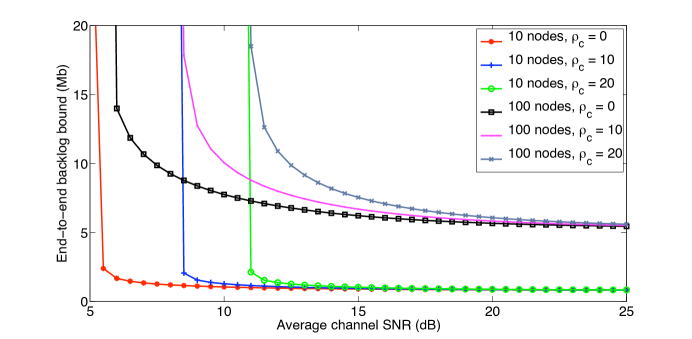
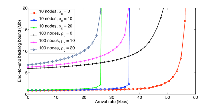
Figure 13: End-to-end backlog bound ($b_{o,{\rm net}}^{\varepsilon}$) vs. average channel SNR ($\bar{\gamma}$) for multi-hop Rayleigh fading channels with $\varepsilon=10^{-4}$, $N=10$ and $100$, $(\sigma(s),\rho(s))$ bounded traffic with $\sigma_{o}(s)=50$ kb, $\rho_{o}(s)=30$ kbps, $(\sigma(s),\rho(s))$ bounded cross traffic with $\sigma_{c}(s)=50$ kb and $\rho_{c}(s)=0,10,20$, and $W=20$ kHz.

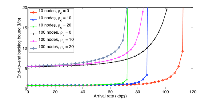
Figure 14: End-to-end backlog bound ($b_{o,{\rm net}}^{\varepsilon}$) vs. arrival rate ($\rho_{o}(s)$) for multi-hop Rayleigh fading channels with $\varepsilon=10^{-4}$, $(\sigma(s),\rho(s))$ bounded traffic with $\sigma_{o}(s)=50$ kb, $(\sigma(s),\rho(s))$ bounded cross traffic with $\sigma_{c}(s)=50$ kb and $\rho_{c}(s)=0,10,20$, $\bar{\gamma}=10$ dB, and $W=20$ kHz.

Figure 15: End-to-end backlog bound ($b_{o,{\rm net}}^{\varepsilon}$) vs. arrival rate ($\rho_{o}(s)$) for multi-hop Rayleigh fading channels with $\varepsilon=10^{-4}$, $(\sigma(s),\rho(s))$ bounded traffic with $\sigma_{o}(s)=50$ kb, $(\sigma(s),\rho(s))$ bounded cross traffic with $\sigma_{c}(s)=50$ kb and $\rho_{c}(s)=0,10,20$, $\bar{\gamma}=20$ dB, and $W=20$ kHz.

VI-B Numerical Examples

We now present numerical examples for Rayleigh fading channels. We use the same traffic and channel model as in the numerical examples in Sec. V-B. The cross traffic is $(\sigma(s),\rho(s))$ bounded traffic with parameters $\sigma_{c}(s)$ and $\rho_{c}(s)$. As before, we assume that cross traffic is deterministically bounded by using fixed values for $\sigma_{c}(s)$ and $\rho_{c}(s)$. Consequently, there is no statistical multiplexing between through and cross traffic. Throughout, the violation probability is set to $\varepsilon=10^{-4}$.

In Fig. 15 we show the end-to-end backlog bound $b_{o,{\rm net}}^{\varepsilon}$ as a function of the average channel SNR $\bar{\gamma}$. The through flow has fixed parameters $\sigma_{o}(s)=50$ kb and $\rho_{o}(s)=30$ kbps, and the cross traffic has parameters $\sigma_{c}(s)=50$ kb and $\rho_{c}(s)=0,10,20$. We consider networks with $N=10$ and $N=100$ nodes. The graph illustrates how the bursts of the cross traffic contribute to the backlog bound. There is an additive component for each traversed channel, which explains the difference for the backlog with $10$ and $100$ channels. The minimum required SNR needed for stability appears less sensitive to the number of channels.

In Figs. 15 and 15 we again evaluate the end-to-end backlog bound $b_{o,{\rm net}}^{\varepsilon}$. Here, we keep the channel SNR values constant at $\bar{\gamma}=10$ (Fig. 15) and $\bar{\gamma}=20$ (Fig. 15). We vary the rate of the through flow $\rho_{o}(s)$ on the x axis, and plot graphs for different values of $\rho_{c}(s)=0,10,20$. We again consider $N=10$ and $N=100$. The outcomes are as seen in the previous figure. We observe the effects of the additive component contributed by each node. Also, we observe, at least for lower transmission rates, that the stability of end-to-end backlogs is not sensitive to the number of traversed channels.

VII Conclusion

We have developed a novel network calculus that can incorporate fading channel distributions, without the need for secondary models, such as FSMC. We use the calculus to compute statistical bounds on delay and backlog of multi-hop wireless networks with fading channels. We took a fresh point of view, where the descriptions of the arrivals and the fading channels reside in different domains, referred to as bit domain and SNR domain. We found that by mapping arrival processes to the SNR domain, an end-to-end analysis with fading channels becomes tractable. An important discovery was that arrivals and service in the SNR domain obey the laws of a $(\min,\times)$ dioid algebra.

The analytical framework developed in this paper appears suitable to study a broad class of fading channels and their impact on the network-layer performance in wireless networks. Even though we computed numerical examples for very simplified networks, in particular, we made strong independence assumptions for the fading channels, our $(\min,\times)$ network calculus is applicable to networks where these assumptions are relaxed. Generalizing our framework and obtaining a more profound understanding of the dioid algebra and computational methods in the SNR domain is the subject of future research.

References

- [1] T. N. A. Alfa and J. Cai. A weighted queue-based model for correlated Rayleigh and Rician fading channels. IEEE Trans. on Communications, 59(11):3049–3058, Nov. 2011.
- [2] G. Amarasuriya, C. Tellambura, and M. Ardakani. Asymptotically-exact performance bounds of AF multi-hop relaying over Nakagami fading. IEEE Trans. Commun., 59(4):962–967, April 2011.
- [3] N. Bisnik and A. A. Abouzeid. Queuing network models for delay analysis of multihop wireless ad hoc networks. Elsevier Ad Hoc Networks, 7(1):79–97, January 2009.
- [4] A. Burchard, J. Liebeherr, and S. Patek. A min-plus calculus for end-to-end statistical service guarantees. IEEE Trans. on Information Theory, 52(9):4105–4114, September 2006.
- [5] C.-S. Chang. Performance guarantees in communication networks. Springer Verlag, 2000.
- [6] C.-S. Chang and R. L. Cruz. A time varying filtering theory for constrained traffic regulation and dynamic service guarantees. In Proc. IEEE Infocom, pages 63–70, 1999.
- [7] Y. Chen, Y. Yang, and I. Darwazeh. A cross-layer analytical model of end-to-end delay performance for wireless multi-hop environments. In Proc. IEEE Globecom, pages 1–6, December 2010.
- [8] J. Choe and N. B. Shroff. A central-limit-theorem-based approach for analyzing queue behavior in high-speed networks. IEEE/ACM Transactions on Networking, 6:659–671, 1998.
- [9] F. Ciucu. Non-asymptotic capacity and delay analysis of mobile wireless networks. In Proc. ACM Sigmetrics, pages 359–360, June 2011.
- [10] F. Ciucu, P. Hui, and O. Hohlfeld. Non-asymptotic throughput and delay distributions in multi-hop wireless networks. In Proc. 48th Annual Allerton Conf. on Communication, Control, and Computing, pages 662–669, Sep. 2010.
- [11] B. Davies. Integral transforms and their applications. Springer-Verlag, NY, 1978.
- [12] E. Elliott. Estimates of error rates for codes on burst-noise channels. Bell System Technical Journal, 42(5):1977–1997, September 1963.
- [13] M. Fidler. An end-to-end probabilistic network calculus with moment generating functions. In Proc. IEEE IWQoS, pages 261–270, June 2006.
- [14] M. Fidler. A network calculus approach to probabilistic quality of service analysis of fading channels. In Proc. IEEE Globecom, pages 1–6, Nov. 2006.
- [15] P. Giacomazzi and G. Saddemi. Bounded-variance network calculus: Computation of tight approximations of end-to-end delay. In Proc. IEEE ICC, pages 170–175, May 2008.
- [16] E. Gilbert. Capacity of a burst-noise channel. Bell System Technical Journal, 39(9):1253–1265, September 1960.
- [17] M. O. Hasna and M. S. Alouini. Outage probability of multihop transmission over Nakagami fading channels. IEEE Commun. Lett., 7(5):216–218, 2003.
- [18] M. Hassan, M. M. Krunz, and I. Matta. Markov-based channel characterization for tractable performance analysis in wireless packet networks. IEEE Trans. Wireless Commun., 3(3):821–831, 2004.
- [19] F. Ishizaki and H. G. Uk. Queuing delay analysis for packet schedulers with/without multiuser diversity over a fading channel. IEEE Trans. Veh. Technol., 56(5):3220–3227, 2007.
- [20] Y. Jiang and P. J. Emstad. Analysis of stochastic service guarantees in communication networks: a server model. In Proc. IWQoS, Springer Lecture Notes in Computer Science 3552, pages 233–245, June 2005.
- [21] Y. Jiang and Y. Liu. Stochastic network calculus. Springer, 2008.
- [22] F. Kelly. Notes on effective bandwidths. In Stochastic Networks: Theory and Applications. (Editors: F.P. Kelly, S. Zachary and I.B. Ziedins) Royal Statistical Society Lecture Notes Series, 4, pages 141–168. Oxford University Press, 1996.
- [23] L. Le and E. Hossain. Tandem queue models with applications to QoS routing in multihop wireless networks. IEEE Trans. Mobile Comput., 7:1025–1040, 2008.
- [24] L. Le, A. Nguyen, and E. Hossain. A tandem queue model for performance analysis in multihop wireless networks. In Proc. IEEE WCNC, pages 2981–2985, March 2007.
- [25] J. Le Boudec and P. Thiran. Network calculus: a theory of deterministic queuing systems for the Internet. Lecture Notes in Computer Science 2050. Springer, 2001.
- [26] C. Li, A. Burchard, and J. Liebeherr. A network calculus with effective bandwidth. IEEE/ACM Trans. on Networking, 15(6):1442–1453, Dec. 2007.
- [27] C. Li, H. Che, and S. Li. A wireless channel capacity model for quality of service. IEEE Trans. Wireless Commun., 6(1):356–366, 2007.
- [28] K. Mahmood, A. Rizk, and Y. Jiang. On the flow-level delay of a spatial multiplexing MIMO wireless channel. In Proc. IEEE ICC, pages 1–6, June 2011.
- [29] K. Mahmood, M. Vehkaperä, and Y. Jiang. Cross-layer modeling of randomly spread CDMA using stochastic network calculus. http://arxiv.org/abs/1105.0215, 2011.
- [30] J. Proakis and M. Salehi. Digital Communications (5th Ed.). McGraw Hill, 2007.
- [31] P. Sadeghi, R. Kennedy, P. Rapajic, and R. Shams. Finite-state Markov modeling of fading channels – a survey of principles and applications. IEEE Signal Process. Mag., 25(5):57–80, 2008.
- [32] T. A. Tsiftsis. Performance of wireless multihop communications systems with cooperative diversity over fading channels. Wiley Int. J. Communication Systems, 21(5):559–565, 2008.
- [33] G. Verticale. A closed-form expression for queuing delay in Rayleigh fading channels using stochastic network calculus. In Proc. ACM Q2SWinet ’09, pages 8–12, 2009.
- [34] G. Verticale and P. Giacomazzi. An analytical expression for service curves of fading channels. In Proc. IEEE Globecom, pages 635–640, Nov. 2009.
- [35] H. Wang and N. Moayeri. Finite-state Markov channel - a useful model for radio communication channels. IEEE Trans. Veh. Technol., 44(1):163–171, 1995.
- [36] Q. Wang, D. Wu, and P. Fan. Effective capacity of a correlated Nakagami-m fading channel. Wirel. Commun. Mob. Comp.. DOI: 10.1002/wcm.1048, 2011.
- [37] Q. Wang, D. Wu, and P. Fan. Effective capacity of a correlated Rayleigh fading channel. Wirel. Commun. Mob. Comp.. DOI: 10.1002/wcm.945, 11(11):1485–1494, 2011.
- [38] D. Wu and R. Negi. Effective capacity: a wireless link model for support of quality of service. IEEE Trans. Wireless Commun., 2(4):630–643, 2003.
- [39] D. Wu and R. Negi. Effective capacity-based quality of service measures for wireless networks. J. on Mobile Networking and Applications, 11(1):91–99, February 2006.
- [40] K. Zheng, L. Lei, Y. Wang, Y. Lin, and W. Wang. Quality-of-service performance bounds in wireless multi-hop relaying networks. IET Communications, 5(1):71–78, Jan. 2011.
- [41] L. Zhong, F. Alajaji, and G. Takahara. A binary communication channel with memory based on a finite queue. IEEE Trans. Information Theory, 53(8):2815–2840, August 2007.
- [42] M. Zorzi, R. Rao, and L. Milstein. On the accuracy of a first-order Markov model for data transmission on fading channels. In Proc. IEEE ICPUC, pages 211–215, November 1995.