Economics of WiFi Offloading:
Trading Delay for Cellular Capacity

Abstract

Cellular networks are facing severe traffic overloads due to the proliferation of smart handheld devices and traffic-hungry applications. A cost-effective and practical solution is to offload cellular data through WiFi. Recent theoretical and experimental studies show that a scheme, referred to as delayed WiFi offloading, can significantly save the cellular capacity by delaying users’ data and exploiting mobility and thus increasing chance of meeting WiFi APs (Access Points). Despite a huge potential of WiFi offloading in alleviating mobile data explosion, its success largely depends on the economic incentives provided to users and operators to deploy and use delayed offloading. In this paper, we study how much economic benefits can be generated due to delayed WiFi offloading, by modeling a market based on a two-stage sequential game between a monopoly provider and users. We also provide extensive numerical results computed using a set of parameters from the real traces and Cisco’s projection of traffic statistics in year 2015. In both analytical and numerical results, we model a variety of practical scenarios and control knobs in terms of traffic demand and willingness to pay of users, spatio-temporal dependence of pricing and traffic, and diverse pricing and delay tolerance. We demonstrate that delayed WiFi offloading has considerable economic benefits, where the increase ranges from 21% to 152% in the provider’s revenue, and from 73% to 319% in the users’ surplus, compared to on-the-spot WiFi offloading.

I Introduction

Mobile data traffic is growing enormously, as smart phones/pads equipped with high computing powers and diverse applications are becoming popular. Cisco reported that global mobile data traffic grew 2.3-fold in 2011, more than doubling for the four consecutive years, which supports its previous annual forecast since 2008 [1]. It was also forecast there that the total global mobile data traffic will increase 18-fold between 2011 and 2016, where the average smartphone is projected to generate 1.3 GB per month in 2015 [1]. To cope with such mobile data explosion, upgrading to 4G (e.g., LTE (Long Term Evolution) or WiMax), may be an immediate solution, but mobile applications are becoming more diverse with larger data consumption and the number of smartphone/pad users are also increasing rapidly. Then, users’ traffic demand is expected to exceed the capacity of 4G in the near future, and thus mobile network operators keep seeking other alternatives to efficiently respond to data explosion [2, 3].

WiFi offloading, where users use WiFi prior to 3G/4G whenever they have data to transmit/receive, has been proposed as a practical solution that can be applied without much financial burden in practice. Network operators as well as users can easily and quickly install WiFi access points (APs) with low costs, and in fact many operators worldwide have already deployed and provided WiFi services in hot-spots and residential areas. Recent papers [4, 5] demonstrate that a huge portion of cellular traffic can be offloaded to WiFi by letting users delay their delay-tolerant data (e.g., movie, software downloads, cloud backup and sync services), and upload/download data whenever they meet a WiFi AP within a pre-specified delay deadline. We call this delayed WiFi offloading, and about 60-80% of cellular traffic can be reduced when 30 mins to 1 hour delay for human mobility [4] and 10 mins of delay for vehicular mobility [5] are allowed. This remarkable offloading efficiency is due to users’ mobility enabling themselves to be under a WiFi coverage during a considerable portion of their business time. Example usage scenarios include: 1) Alice records video of a family outing at a park using her cell phone and wants to archive it in her data storage in the Internet. She does not need the video immediately until she comes back home in several hours. 2) Bob will travel this afternoon from New York to Los Angeles and he just realizes that he can use some entertainment during the long flight. As he has several hours before the trip, he schedules to download a couple of movies on his cell phones.

However, WiFi offloading’s high potential does not always guarantee that users and providers adopt it in practice. First, users may be reluctant to delay their traffic without economic incentives, e.g., discounted service fees. For example, if a user pays based on an unlimited data plan, which is still a popular payment plan worldwide, users may have no reason to delay traffic unless WiFi-required services, e.g., services requiring higher bandwidths, are necessary. Also, operators may not always welcome delayed offloading service, since the total cellular traffic to charge may decrease, possibly leading to its revenue reduction. Thus, it is of significant importance to formally address the question on the economic gains of delayed WiFi offloading from the perspective of users, operators, and regulators, which is the focus of this paper.

In this paper, we model a market with a monopoly operator and users based on a two-stage sequential game, where the operator controls the price and users are price-takers. A variety of control knobs will show different economic impacts of delayed WiFi offloading. Our major focus is to understand how and how much users and the provider obtain the economic incentives by adopting delayed WiFi offloading and study the effect of different pricing and delay-tolerance. The major features of our model include four different pricing schemes (flat, volume, two-tier, and congestion) and heterogeneous users in terms of traffic demands and willingness to pay.

Using the market model mentioned above, we first conduct analytical studies under flat and volume pricing for the simple cases when the traffic demand follows a certain distribution (obtained from the measurement studies), and users are uniformly distributed among cells. This simplification seems to be unavoidable for mathematical tractability, yet we are able to fundamentally understand how the users and the provider become economically beneficial. We formally prove that delayed WiFi offloading indeed generates the economic incentives for the users and the provider. To obtain more practical messages and quantify the gain of delayed WiFi offloading, we use two traces, each of which tells us the information on cellular data usage and WiFi connectivity. We extract the parameters needed by our model from those traces, and obtain numerical results, from which, we draw the following key messages:

1. WiFi offloading is economically beneficial for both the provider and users, where depending on the pricing schemes and delay tolerance, the increase ranges from 21% to 152% in the provider’s revenue and from 73% to 319% in the users’ surplus.

2. Revenue in volume pricing exceeds that in flat pricing. However, the revenue increasing rate of delayed offloading in flat pricing is higher than that in volume pricing.

3. Pricing with higher granularity such as two-tier and congestion pricing increases the revenue, compared to flat and volume pricing, but the gains become smaller as offloading efficiency increases (i.e., as users delay more traffic).

4. The revenue gain from on-the-spot to delayed offloading is similar to that generated by the network upgrade from 3G to 4G.

II Related Work

There have been several works [4, 5, 6] on delayed WiFi offloading. Lee et al. [4] proposed a delayed offloading framework, where users specify a deadline for each application or data, and each delay tolerant data is served in a shortest remaining time first (SRTF) manner through WiFi networks. If the delay deadline of the data expires, then the data is transmitted through 3G networks. On real human mobility traces, it is shown that 80% of cellular traffic can be offloaded to WiFi networks when 1 hour delay is allowed. Balasubramanian et al. [5] proposed an offloading framework for vehicular networks, which supports fast switching between 3G and WiFi, and avoids bursty WiFi losses. They demonstrated that more than 50% of cellular traffic can be reduced for a delay tolerance of 100 seconds on vehicular mobility. Hultell et al. [6] addressed the user experienced performance of delayed transmission and proposed context-aware caching/prefetching to provide users immediate services, e.g. web browsing, news, and streaming. They found that more than 80% of news can be pre-fetched within 700 seconds, with only 50 WiFi APs per km² (1.2% spatial coverage) on a random mobility model. Therefore, WiFi networks are proven to offload large fraction of cellular data for various mobility conditions and low AP density, whenever data can tolerate some amount of delay.

Some recent works [7, 8] devised incentive frameworks for users to delay their data traffic. Ha et al. [7] proposed a time-dependent pricing scheme for mobile data, which incentivizes users to delay their traffic from the higher- to lower-price time zone. They conducted surveys which revealed that users are indeed willing to wait 5 minutes (for YouTube videos) to 48 hours (for software updates). They addressed that the time-dependent pricing flattens temporal fluctuation of traffic usage and benefits wireless operators. In [8], Zhuo et al. proposed an incentive framework for downlink mobile traffic offloading based on an auction mechanism, where users send bids, which include the delay it can tolerate and the discount the user wants to obtain for that delay, and the provider buys the delay tolerance from the users. However, previous studies did not provide how much economic gain the provider and users can obtain. In this paper, we quantify the economic gain of delayed offloading based on real-world traces.

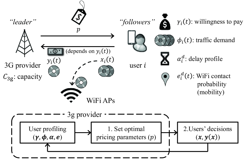
Figure 1: An illustration of the system model. $x_{i}(t)$ and $y_{i}(t)$ are 3G+WiFi and 3G traffic volumes of user $i$ at time $t.$ Note that $x_{i}(t)\leq\phi_{i}(t).$

III Model

We illustrate the system model in Fig. 1. We model users with four attributes, (i) how much money they can pay (willingness to pay, $\bm{\gamma}$), (ii) how much data they want to use (traffic demand, $\bm{\phi}$), (iii) how long their data can tolerate (delay profile, $\bm{\alpha}$), and (iv) how they move (WiFi contact probability, $\bm{e}$). We index users by $i$, time slots by $t$, and deadlines by $d.$ Assuming that the monopoly provider knows users’ attributes and strategies a priori, we model a market model based on a two-stage sequential game (e.g. Stackelberg game). At the first stage, the provider decides on the pricing parameters ($p$) (for a fixed pricing scheme, which we will describe later) as a leader, and at the second stage, each user is a price-taker as a follower and chooses the 3G+WiFi traffic volume $\bm{x}.$ Our analysis and numerical results are carried out based on the equilibrium of this game. We describe the detailed network, traffic, and market models in the following subsections.We summarize major notations in Table I.

III-A Network and Traffic Model

III-A1 Network model

We consider a network consisting of cellular base stations (BSs) and WiFi APs, where $N$ users are served by the cellular provider. Users are always guaranteed to be under the coverage of a cellular BS, but not necessarily of a WiFi AP. We consider a one-day time scale whose average analysis over the unit billing cycle, e.g., one month, is presented. A day is divided into time slots $t\in\{1,2,\ldots,T\},$ where $T$ is the last index of one day, depending on the duration of a time slot. Let $C_{\text{3g}}$ be the capacity (in volume per slot) provided by a BS. During each day, users move among BSs as well as APs. Let $e_{i}^{d}(t)$ be the probability that user $i$ meets any WiFi AP within deadline $d$ at time slot $t.$ For instance, $e_{i}^{\text{1hour}}(\text{13:00})=0.7$ means that user $i$ meets a WiFi AP from 1 p.m. to 2 p.m. with probability 0.7. The value of $e_{i}^{d}(t)$ can be obtained by analyzing user $i$’s mobility trace during, say, a month. We assume that only 3G traffic is charged. Each user has its own set of accessible, free WiFi APs, e.g., ones in home, office, or hotspots, deployed by users, users’ companies, providers, or governments. We ignore the cost from offloaded data since the cost of accessing the Internet via a WiFi AP connected to a wired network is considerably lower than that for accessing the cellular network [9].

TABLE I: Summary of Major Notation

Variable	Definition
$N$ and $C_{\text{3g}}$	Number of users and Capacity of a BS cell
$\theta$	Price sensitivity
$e_{i}^{d}(t)$	The WiFi contact probability of user $i$
	at slot $t$ within deadline $d$
$\alpha_{i}^{d}$	Portion of traffic of user $i$ with deadline $d$
$x_{i}(t)$	3G+WiFi traffic volume of user $i$ at slot $t$
$y_{i}(t)$	3G traffic volume of user $i$ at slot $t$
$\phi_{i}(t)$	Traffic demand of user $i$ at slot $t$
$w_{i}(t)$	Temporal preference (weight) of user $i$ at time $t$
$\gamma_{i}(t)$	Willingness to pay of user $i$ for traffic at time $t$

III-A2 Traffic model

We assume that user $i$ has the average daily traffic demand ${\Phi}_{i},$ 3G+WiFi traffic vector $\bm{x}_{i}=(x_{i}(t):t\in T),$ and 3G traffic vector $\bm{y}_{i}(\bm{x}_{i})=(y_{i}(t):t\in T),$ where $x_{i}(t)$ is the traffic volume of user $i$ generated at slot $t$, transferred through either 3G or WiFi, and $y_{i}(t)$ is the traffic volume transferred through only 3G. The daily traffic demand ${\Phi}_{i}$ is temporally split into $\bm{\phi}_{i}=(\phi_{i}(t):t\in T),$ where $\phi_{i}(t)$ is traffic demand at slot $t,$ and ${\Phi}_{i}=\sum_{t\in T}\phi_{i}(t).$ The traffic volume of user $i$ at slot $t$ is constrained by the traffic demand, i.e., $x_{i}(t)\leq\phi_{i}(t).$ We denote $w_{i}(t)=\frac{\phi_{i}(t)}{{\Phi}_{i}}$ as temporal preference (weight) of user $i$. For example, for a user $i$’s traffic demand 1 GB, where users want to send 700 MB at daytime an 300 MB at nighttime (i.e., just two time slots), $\phi_{i}(\text{day})=700$ and $\phi_{i}(\text{night})=300,$ and $w_{i}(\text{day})=0.7$ and $w_{i}(\text{night})=0.3.$ Users may not be able to deliver all traffic demand, and the actual transmitted volume depends on the price and user utility, which we will describe later. The traffic volume for 3G, $\bm{y}_{i}$ which is actually charged, relies on $\bm{x}_{i}$ as well as each user $i$’s mobility and delay profile, which we define in the following paragraph.

We introduce a notion of delay profile to model per-user delay-tolerance of traffic. The delay profile is denoted by $\bm{\alpha}=(\alpha_{i}^{d}:i\in N,d\in\{0,1,...,D\})$ such that $\sum_{d=0}^{D}\alpha_{i}^{d}=1,$ where $\alpha_{i}^{d}$ is the portion of user $i$’s traffic demand that allows deadline $d$, and $D$ is the maximum allowable deadline across all traffic. For example, for a user $i$’s traffic demand 1 GB, if the user has 300 MB, 700 MB, allowing 10 mins and 1 hour, resp., we have $\alpha_{i}^{\text{10m}}=0.3,$ $\alpha_{i}^{\text{1h}}=0.7.$ For example, for a user $i$’s traffic demand 1 GB, if the user has 100 MB, 200 MB, 700 MB, allowing real-time, 10 mins, and 1 hour, respectively, we have $\alpha_{i}^{0}=0.1,$ $\alpha_{i}^{\text{10m}}=0.2,$ $\alpha_{i}^{\text{1h}}=0.7.$ For a given per-user delay profile, each user uses only WiFi connections to deliver some data until the allowable deadline expires, after which the remaining data is immediately transferred through 3G. In particular, when no delay is allowed ($\alpha_{i}^{0}=1$), we call this regime on-the-spot offloading, where a user only uses spontaneous connectivity of WiFi. Most current smartphones support this by default.

III-B Market Model

We start by explaining the economic metrics of the users and the provider. We assume that the provider and users are rational and try to maximize revenue and net-utility.

III-B1 Users and Provider

We model heterogeneous willingness to pay among users over time slots, which we denote by $\gamma_{i}(t)\geq 0$ for user $i$ at time $t.$ For an average user $i,$ $\gamma_{i}(t)$ tends to be higher when $t$ is in daytime. We first define user $i$’s utility at time slot $t$ by $\gamma_{i}(t)x_{i}(t)^{\theta},$ where the constant $\theta\in(0,1)$ is price-sensitivity. The utility function $\gamma_{i}(t)x_{i}(t)^{\theta}$ is called an iso-elastic function with the property of an increasing function of traffic volume $x_{i}(t)$ for all $i$ and $t$, but of a decreasing marginal payoff. Then, user $i$’s (aggregate) net-utility $U_{i}(\bm{x}_{i})$ during a day is:

$$U_{i}(\bm{x}_{i})=\sum_{t\in T}\gamma_{i}(t)x_{i}(t)^{\theta}-m\big{(}p,\bm{y}_{i}(\bm{x}_{i})\big{)},$$

where $m(p,\bm{y}_{i}(\bm{x}_{i}))$ is the daily payment charged by the provider whose price is $p$. We abuse the notation and use $p$ to refer to the pricing parameters of a given pricing scheme, and the function form of $m$ differs depending on a pricing scheme (see Section III-B2). Recall the notation $\bm{y}_{i}(\bm{x}_{i})$ represents the dependency of the 3G traffic on 3G+WiFi traffic.

Given the traffic demand $\bm{\phi}_{i},$ mobility pattern, willingness to pay $\bm{\gamma}_{i}=(\gamma_{i}(t):t\in T)$, delay profile $\alpha_{i}^{d}$, and a pricing scheme (and its parameters), each user $i$ chooses $\bm{x}^{\star}_{i}$ to maximize his/her net-utility,

$${\bf User:} \displaystyle\max_{{x}_{i}(t)\leq\phi_{i}(t),\ \forall t\in T}U_{i}(\bm{x}_{i}),$$ (1)

where each user $i$ subscribes to 3G service only if the net-utility is positive, i.e., $U_{i}(\bm{x}_{i})>0.$

Under a given pricing scheme, the provider decides on the price (more precisely, the parameters of the pricing scheme) to maximize its expected revenue, $R(p)$:

$${\bf Provider:} \displaystyle\max_{p\in\mathcal{P}}R(p),$$ (2)

where $\mathcal{P}$ is the set of all feasible prices such that (i) the revenue is positive (provider rationality), and (ii) the expected 3G traffic volume at each time and at each BS cell is smaller than 3G capacity $C_{\text{3g}}$ (capacity constraint).

The expected revenue $R(p)$ is the total income minus cost,

$$R(p)=\sum_{i\in N}m\big{(}p,\bm{y}_{i}(\bm{x}_{i})\big{)}-\sum_{i\in N}c\big{(}\bm{y}_{i}(\bm{x}_{i})\big{)},$$ (3)

where $c(\bm{y}_{i})$ is the network cost to handle the 3G traffic, which we model by a linearly increasing function, $c(\bm{y}_{i})=\eta\sum_{t\in T}y_{i}(t),$ where $\eta$ is the cost of the unit volume of the 3G traffic. The cost term captures the money for operation and maintenance including electric power costs as well as customer complaints due to congestion. The linearly increasing network cost is commonly used in the analysis of cellular cost [10]. We ignore the backhaul cost of both 3G and WiFi networks. User surplus $S$ is the summation of users’ net-utility and social welfare $W$ is the summation of user surplus and provider revenue, or,

$$S = \sum_{i\in N}U_{i}(\bm{x}_{i}),$$

$$W = \sum_{i\in N,t\in T}\gamma_{i}(t)x_{i}(t)^{\theta}-\sum_{i\in N}c\big{(}\bm{y}_{i}(\bm{x}_{i})\big{)}.$$

III-B2 Pricing

For a given pricing scheme, the 3G provider fixes a price parameter which is announced to the users. We consider four pricing schemes - flat, two-tier, volume, and congestion - that are popularly studied in literature. Each pricing scheme has tunable parameters controlled by the provider: $\{p_{f}\},~{}\{p_{t}^{1},p_{t}^{2},y_{\text{max}}^{1}\},$ $\{p_{v}\},$ and $\{p_{v}(t,s)\},$ which we elaborate shortly. For a given pricing scheme and its price parameters $p$, a user with 3G traffic volume $\bm{y}_{i}$ pays $m\big{(}p,\bm{y}_{i}\big{)}$ to the provider. Note that if a user does not subscribe or generate any traffic, the payment is zero, i.e., $m\big{(}p,\bm{0}\big{)}=0.$

Flat. The provider offers unlimited service for users who pay a subscription fee $p_{f}$.

Two-tier. Multiple price points are provided for several usage options. For example, AT&T has a pricing plan that offers up to 300 MB, 3 GB, and 5 GB for $20, $30, and $50 per month, respectively. In this paper, we consider two price points, where the provider offers maximum daily traffic volume $y^{1}_{\max}$ for fixed fee $p_{t}^{1}$ and unlimited service for fixed fee $p_{t}^{2}$, or,

$$m\big{(}p,\bm{y}_{i}\big{)} = \begin{cases}p_{t}^{1},&\mbox{if }\quad 0<\sum_{t\in T}y_{i}(t)\leq y^{1}_{\max}.\\ p_{t}^{2},&\mbox{if }\quad\sum_{t\in T}y_{i}(t)>y^{1}_{\max}.\end{cases}$$

Volume. A user is charged to pay $p_{v}$ for the unit 3G traffic volume, or,

$$m\big{(}p,\bm{y}_{i}\big{)} = p_{v}\cdot\sum_{t\in T}y_{i}(t).$$

Congestion. We consider a volume-based congestion pricing, or simply congestion pricing in this paper, where the price for a unit file size varies with time and location, or,

$$m\big{(}p,\bm{y}_{i}\big{)}=\sum_{t\in T}{p_{v}(t,s_{i}(t))\cdot y_{i}(t)},$$

where $p_{v}(t,s)$ is the unit price at time slot $t$ and cell $s,$ and $s_{i}(t)$ is the cell id with which user $i$ is associated at $t.$

We note that in flat and two-tier pricing, users do not subscribe to the service when the net-utilities are not positive, which is the major factor determining the provider’s revenue, whereas in volume and congestion pricing, every user subscribes and just controls its traffic volume. Two-tier and congestion pricing schemes are the extensions of flat (in terms of price granularity) and volume (in terms of space and time), resp. Tiered pricing in mobile data services is popularly used recently [1] as the provider can set up multiple pricing points, while maintaining simplicity in the pricing structure. Congestion pricing has been considered as a way of revenue increase in networking services (see e.g., [7, 11, 12]). In fact, in the usage of cellular networks, it has been reported that spatial and temporal variation of mobile data traffic are shown to be remarkable [13], implying high potential in the increase of the provider’s revenue and better resource utilization. Despite the high billing complexity, it is interesting to see its quantified impact in WiFi offloading.

IV Analysis of WiFi Offloading Market

In Sections IV-B and IV-C, we provide analytical studies of the economic gain of WiFi offloading. Due to complex interplays among pricing parameters, and more importantly users’ heterogeneity, our analysis is made under several assumptions. This simplification seems unavoidable for mathematical tractability, yet we are able to understand how the users and the provider become economically beneficial. Note that in Section V, we quantify economic gains of WiFi offloading in more practical settings (heterogeneous cells and willingness to pay of users) as well as complex pricing schemes (two-tier and congestion).

IV-A Assumptions and Definitions

1. Homogeneous cells. User associations are uniformly distributed among cells so that it suffices to consider only a single BS cell, where the number of users is $\hat{N}=N/(\text{\# of cells})$. The distribution of users’ traffic demand in each cell is identical.

2. Traffic demand distribution. In each cell, the daily traffic demand $\Phi_{i}$ follows a random variable $\Phi$ which follows an upper-truncated power-law distribution, given by: $f_{{\Phi}}(x)={x^{-\sigma}}/{Z},$ for $0\leq x\leq{\Phi}_{\max}$, where $\sigma$ is the exponent, ${\Phi}_{\max}$ is the maximum value of ${\Phi},$ and $Z=\frac{{\Phi}_{\max}^{1-\sigma}}{1-\sigma}$ with $0<\sigma<1.$

3. Willingness to pay and temporal preference. Users are homogeneous in willingness to pay and temporal preference, i.e., $\gamma_{i}(t)=\gamma(t),w_{i}(t)=w(t),~{}\forall i\in N,~{}t\in T.$ In regard to willingness to pay, we let $\gamma(t)=w(t)^{1-\theta}.$ However user’s traffic demand is heterogeneous as in A2.

4. Pricing. We consider only flat and volume pricing. Thus, throughout this section, the pricing parameter $p$ refers to the flat fee $p_{f}$ and the unit price $p_{v}$ in each pricing, resp.

In A2, we comment that in recent measurement studies [13, 14], the traffic volume distribution of cellular devices is shown to follow an upper-truncated power-law distribution. Especially, in [13], the adopted pricing policy was flat pricing, so that the measured traffic usage was not affected by pricing. Thus, we apply an upper-truncated power-law distribution to daily traffic demand ${\Phi}.$ In A3, willingness to pay $\gamma(t)$ at time $t$ is set, such that at each time slot $t$ (i) one has larger willingness to pay for larger traffic demand and (ii) utility generated by traffic demand ($\gamma(t)\phi(t)^{\theta}$) is proportional to the traffic demand ($\phi(t)=w(t)\Phi$).

Remark IV.1

User heterogeneity only comes from traffic demand $\Phi$ from our assumptions. For notational simplicity, we omit user subscript $i$ and use subscript ${\Phi}$ to represent the user variables with traffic demand ${\Phi},$ e.g., $x_{\Phi}(t),y_{\Phi}(t),$ etc.

Offloading indicators. We first introduce two indicators to quantify how much 3G data is offloaded: (i) aggregate 3G traffic ratio $\kappa_{\text{avg}}$ and (ii) peak 3G traffic ratio $\kappa_{\text{peak}}$.

Definition IV.1 (offloading indicators)

$$\kappa_{\text{avg}}\triangleq\frac{\sum_{t\in T}Y(t)}{\sum_{t\in T}X(t)},\qquad\kappa_{\text{peak}}\triangleq\frac{\max_{t\in T}Y(t)}{\sum_{t\in T}X(t)},$$ (4)

where the transmitted total traffic and 3G traffic over a cell at time $t$, $X(t)$ and $Y(t)$ are:

$$X(t) = \hat{N}\int_{0}^{\Phi_{\max}}x_{\Phi}(t)\text{d}F_{\Phi},$$

$$Y(t) = \hat{N}\int_{0}^{\Phi_{\max}}\sum_{d=0}^{D}b_{\Phi}^{d}(t-d)x_{\Phi}(t-d)\text{d}F_{\Phi},$$ (5)

and $b_{\Phi}^{d}(t)=\alpha_{\Phi}^{d}\big{(}1-e_{\Phi}^{d}(t)\big{)}$ is the portion of the traffic generated at time $t$ which is transmitted through 3G at time $t+d.$

It is clear that as users delay more traffic, the aggregate 3G traffic ratio $\kappa_{\text{avg}}$ provably decreases, since more traffic can be offloaded through WiFi. Also, the peak 3G ratio $\kappa_{\text{peak}}$ decreases as more traffic at peak time is offloaded. In Section V, we show that both $\kappa_{\text{avg}}$ and $\kappa_{\text{peak}}$ decrease as delay tolerances of users get higher.

Opt-saturated and Opt-unsaturated. We define two notions, opt-saturated and opt-unsaturated, which characterize the regimes under which how much traffic is imposed on the network for the equilibrium price. In general, as traffic demand gets higher compared to the 3G capacity, the network becomes opt-saturated, and vice versa. The main reason for introducing those two notions is because the analysis becomes different depending on the volume of network traffic and the market behaves differently, and thus, the way of increasing the revenue and the net-utility can be differently interpreted. For a formal definition, we first recall that $\mathcal{P}$ is the set of all feasible prices, defined by provider rationality and capacity constraint, or,

$$\mathcal{P}\triangleq\left\{p\mid R(p)>0,Y(t;p)\leq C_{\text{3g}},~{}\forall t\in T\right\}.$$ (6)

Definition IV.2 (Opt-saturated and Opt-unsaturated)

Let $p^{\star}$ be an equilibrium price that maximizes the revenue, i.e., $p^{\star}\in\arg\max_{p\in\mathcal{P}}R(p).$ The network is said to be saturated at $p$, if $\max_{t\in T}Y(t;p)=C_{\text{3g}}.$ For a unique equilibrium price $p^{\star}$, the network is said to be opt-saturated if the network is saturated at $p^{\star},$ and opt-unsaturated otherwise.

Let $p_{0}$ be the threshold price above which all the feasible prices lie, i.e., $p_{0}=\inf_{p\in\mathcal{P}}p.$ For a given price $p$, $R(p)>0$ implies $\max_{t\in T}Y(t;p)>0,$ since no user subscription or no traffic results in zero income to the provider. Note that $p^{\star}$ is not necessarily equal to $p_{0}.$ Let $A(p)=\max_{t\in T}Y(t;p)$ be the total 3G traffic at peak time. Note that $A(p)$ is decreasing in $p.$ Since $A(p)$ is decreasing in $p,$ a feasible price in $\mathcal{P}$ is greater than or equal to $p_{0}.$

IV-B Flat pricing

This subsection considers the impact of offloading when flat pricing is used. In flat pricing, a user pays a flat fee $p$ regardless of its 3G traffic usage if it subscribes to the 3G service. Since there is no incentive to discourage excessive network traffic, the traffic volume generated by a user equals to its traffic demand; $x_{\Phi}(t)=\phi(t)$ for a subscribing user with total traffic demand $\Phi,$ where $\phi(t)$ is the traffic demand at slot $t$ split from $\Phi.$

A user with traffic demand $\Phi$ maximizes its net-utility:

$$\sum_{t\in T}\gamma(t)x_{\Phi}(t)^{\theta}-p=\sum_{t\in T}w(t)^{1-\theta}\phi(t)^{\theta}-p=\Phi^{\theta}-p,$$ (7)

since $\gamma(t)=w(t)^{1-\theta}$ by A3, $x_{\Phi}(t)=\phi(t)$, for all $t$, and the temporal preference $w(t)=\frac{\phi(t)}{\Phi}$. From (3), the provider maximizes its revenue:

$$R(p) = \hat{N}p\int_{p^{\frac{1}{\theta}}}^{\Phi_{\max}}\text{d}F_{\Phi}-\hat{N}\eta\int_{p^{\frac{1}{\theta}}}^{\Phi_{\max}}\Phi\text{d}F_{\Phi}$$ (8)

$$= \hat{N}\int_{p^{\frac{1}{\theta}}}^{\Phi_{\max}}(p-\eta\Phi)\text{d}F_{\Phi},$$

where $p^{1/\theta}$ is the lowest traffic demand of a subscriber (i.e., positive net-utility and thus $\Phi^{\theta}>p$). No users subscribe if the price is too high, i.e., if $p\geq p_{\max}$ from (7), where $p_{\max}=\Phi_{\max}^{\theta}.$ Then, we should have that $\mathcal{P}\subset[0,p_{\max}).$

Our main results, Prop. IV.1 and Theorem IV.1, state how the economic values (e.g. price and revenue) change by offloading. Prop. IV.1 characterizes (i) $R(p)$ and the feasible price set, and (ii) the equilibrium prices in the opt-saturated case and (iii) the opt-unsaturated case. Theorem IV.1 states that offloading is economically beneficial for the users, the provider, and the regulator.

Proposition IV.1 (Equilibrium Price in Flat)

If the cost coefficient $\eta<(\kappa_{\text{avg}}{\Phi}_{\max}^{1-\theta})^{-1},$

1. $R(p)$ is unimodal over $[0,p_{\max}),$ and the feasible price set $\mathcal{P}$ is non-empty and connected.

2. The network is opt-saturated, if $R^{\prime}(p_{0})<0,$ where the unique equilibrium price $p^{\star}=p_{0},$ where $p_{0}={\Phi}_{\max}^{\theta}\left(1-\frac{C_{3g}}{\kappa_{\text{peak}}\hat{N}\mathbb{E}[{\Phi}]}\right)^{\frac{\theta}{2-\sigma}}.$

3. The network is opt-unsaturated, if $R^{\prime}(p_{0})>0,$ where the unique equilibrium price $p^{\star}=p^{\star}(\kappa_{\text{avg}})$ is such that $\frac{\partial R(p)}{\partial p}\big{|}_{p=p^{\star}}=0,$ and $\frac{\partial p^{\star}(\kappa_{\text{avg}})}{\partial\kappa_{\text{avg}}}>0.$

Theorem IV.1 (Economic Gain from Offloading in Flat)

If $\eta<(\kappa_{\text{avg}}{\Phi}_{\max}^{1-\theta})^{-1},$ the net-utilities of all subscribers increase and the provider’s revenue at equilibrium increases (thus the user surplus and the social welfare increase), as (i) $\kappa_{\text{peak}}$ decreases in the opt-saturated case, and (ii) as $\kappa_{\text{avg}}$ decreases in the opt-unsaturated case.

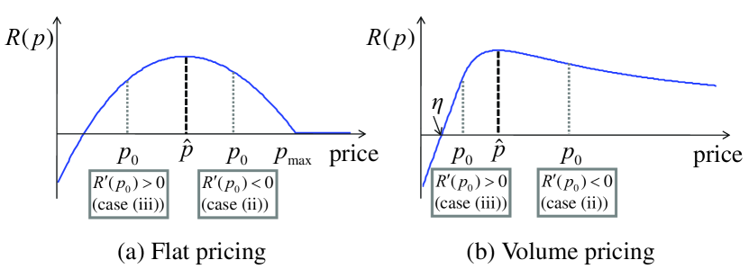
Figure 2: Revenue function $R(p)$ in flat and volume pricing. The $p_{\max}$ is the highest price above which no user subscribes in flat pricing, $\hat{p}$ is the unique solution of $\frac{\partial R(p)}{\partial p}=0,$ and $\eta$ is the network cost coefficient. The achievable revenue (at equilibrium) is not always at $\hat{p}$, since $\hat{p}$ may not be in the feasible price set, which is determined by capacity constraint and provider rationality.

The proof is presented in the Appendix. Here, we briefly interpret Prop. IV.1 and Theorem IV.1. First, clearly if the network cost is too high, the provider cannot achieve any positive revenue, where the condition of $\eta<(\kappa_{\text{avg}}{\Phi}_{\max}^{1-\theta})^{-1}$ guarantees the existence of prices under which the revenue is positive. This condition is relaxed as more offloading occurs (i.e., $\kappa_{\text{avg}}$ decreases), resulting in less restricted business condition with positive revenue from the provider’s perspective. Second, every feasible price is larger than or equal to the threshold price $p_{0}.$ Also, $R(p)$ is unimodal and $\mathcal{P}$ is connected. Thus, at the threshold price, if $R^{\prime}(p_{0})<0,$ then $R(p_{0})\geq R(p)$ for all $p\in\mathcal{P}$ (see Fig. 2(a)). Thus, the equilibrium price is unique, and $p^{\star}=p_{0},$ where $p_{0}$ is characterized as in Prop. IV.1(ii). Also, the network is opt-saturated if $R^{\prime}(p_{0})<0,$, because the peak traffic volume $A(p_{0})=C_{\text{3g}}$ (otherwise, there exists a smaller feasible price than $p_{0}$). Now, if $R^{\prime}(p_{0})>0,$ the equilibrium price $p^{\star}$ is such that $R^{\prime}(p^{\star})=0,$ as in Prop. IV.1(iii). Again, this case makes the network opt-unsaturated because $A(p^{\star})<A(p_{0})$ (due to decreasing property of $A(p)$ in $p$) and $A(p_{0})\leq C_{\text{3g}}.$

We now explain the relationship between traffic demand and opt-saturatedness. The amount of total traffic demand of users affects the revenue change rate at the traffic-maximizing price, $R^{\prime}(p_{0}),$ where 3G capacity and offloading indicators are fixed. If traffic demand is high enough, when the provider can reduce its flat fee (by offloading or network upgrade), revenue increases even with the reduced price, i.e., $R^{\prime}(p_{0})<0,$ since increase of subscribers exceeds price reduction. If traffic demand is not significantly high, subscription ratio does not increase drastically, so that revenue decreases, i.e., $R^{\prime}(p_{0})>0,$ and at the optimal price, the 3G capacity is not fully utilized by the users.

Using the results of Prop. IV.1, Theorem IV.1 states that offloading is economically beneficial from the perspective of the users, the provider, and the regulator, where the mechanisms behind the increase in the revenue are different in the opt-saturated and opt-unsaturated cases. In the opt-saturated case, as more 3G traffic is offloaded through WiFi at peak time, i.e., $\kappa_{\text{peak}}$ decreases, the provider turns out to have extra 3G capacity. Then, the provider attracts more subscribers by lowering its flat fee, in order to utilize the extra capacity. As the increase in the number of subscribers exceeds the reduced price, the revenue increases. Indeed, from Prop. IV.1(ii) the equilibrium price decreases as $\kappa_{\text{peak}}$ decreases. The net-utility increases for all subscribers by price reduction since a subscribing user in flat pricing always generate all the traffic demand. In the opt-unsaturated case, the number of subscribers does not increase drastically even if the provider decreases its flat fee, so that the provider’s income does not increase. However, the network cost decreases substantially as the 3G traffic decreases, i.e., $\kappa_{\text{avg}}$ decreases, and the revenue increases. Since the equilibrium price still decreases, as $\kappa_{\text{avg}}$ decreases from Prop. IV.1(iii), the net-utility increases for all subscribers by the same argument as in the opt-saturated case.

IV-C Volume pricing

In volume pricing, user payment is proportional to its 3G traffic volume. For a given unit price, a user chooses the amount of traffic that maximizes its net-utility. In this subsection, for tractability, we focus more on the average analysis by assuming that per-user and -time dependence of delay profile and WiFi connection probability are homogeneous, i.e., $\alpha_{\Phi}^{d}=\alpha^{d},~{}e_{\Phi}^{d}(t)=e^{d}$ for all $t$ and all users. Then, by (5), for a user with traffic demand $\Phi,$

$$\sum_{t\in T}y_{\Phi}(t)=\sum_{t\in T}\Big{(}x_{\Phi}(t)\sum_{d=0}^{D}\alpha^{d}\big{(}1-e^{d}\big{)}\Big{)}=\kappa_{\text{avg}}\sum_{t\in T}x_{\Phi}(t),$$ (9)

where note that $\kappa_{\text{avg}}=\sum_{d=0}^{D}\alpha^{d}\big{(}1-e^{d}\big{)}$ by the definition in (4). A user with traffic demand $\Phi$ pays $p\sum_{t\in{T}}y_{\Phi}(t)$ and maximizes the following net-utility (for a given price $p$):

$$\quad\quad\sum_{t\in T}\gamma(t){x}_{\Phi}(t)^{\theta}-p\sum_{t\in T}{y}_{\Phi}(t)\cr=\sum_{t\in T}w(t)^{1-\theta}x_{\Phi}(t)^{\theta}-p\kappa_{\text{avg}}\sum_{t\in T}{x}_{\Phi}(t)\quad\quad\quad$$ (10)

using $\gamma(t)=w(t)^{1-\theta}$ and (9). Since users pay in proportion to the volume of 3G traffic, a notion of payment per unit (3G + WiFi) traffic is useful, given by:

$$\frac{p\sum_{t\in T}y_{\Phi}(t)}{\sum_{t\in T}x_{\Phi}(t)}=\frac{p\kappa_{\text{avg}}\sum_{t\in T}x_{\Phi}(t)}{\sum_{t\in T}x_{\Phi}(t)}=p\kappa_{\text{avg}},$$

where without offloading, i.e., $\kappa_{\text{avg}}=1,$ payment per unit traffic is just $p.$ From (3), the provider maximizes its revenue

$$R(p) = \hat{N}(p-\eta)\int_{0}^{\Phi_{\max}}\sum_{t\in T}{y}_{\Phi}(t)\text{d}F_{\Phi}.$$ (11)

Since $R(p)\leq 0$ for $p\leq\eta,$ we should have $\mathcal{P}\subset(\eta,\infty).$ It is clear that as the payment per unit traffic $p\kappa_{\text{avg}}$ decreases, the traffic which can be delivered per dollar increases. We will show that the payment per unit traffic $p\kappa_{\text{avg}}$ decreases, as more offloading through WiFi occurs.

Similarly in flat pricing, we present our main results by Prop. IV.2 and Theorem IV.2. Prop. IV.2 characterizes the equilibrium prices in opt-saturated and opt-unsaturated cases. Theorem IV.2 states that offloading is economically beneficial for the users, the provider, and the regulator.

Proposition IV.2 (Equilibrium Price in Volume)

1. $R(p)$ is unimodal for $p\geq\eta$ and the feasible price set $\mathcal{P}$ is non-empty and connected.

2. The network is opt-saturated, if $R^{\prime}(p_{0})<0,$ where the unique equilibrium price is $p^{\star}=p_{0}$ where $p_{0}=p_{0}(\kappa_{\text{peak}})$ is the threshold price, and $\frac{\partial p_{0}(\kappa_{\text{peak}})}{\partial\kappa_{\text{peak}}}>0.$

3. The network is opt-unsaturated, if $R^{\prime}(p_{0})>0,$ where the unique equilibrium price $p^{\star}=p^{\star}(\kappa_{\text{avg}})$ is such that $\frac{\partial R(p)}{\partial p}\big{|}_{p=p^{\star}}=0,$ and $\frac{\partial(p^{\star}(\kappa_{\text{avg}})\kappa_{\text{avg}})}{\partial\kappa_{\text{avg}}}>0.$

Theorem IV.2 (Economic Gain from Offloading in Volume)

The net-utilities for all users increase and the provider’s revenue increases (thus the user surplus and the social welfare increase), (i) as $\kappa_{\text{peak}}$ decreases, in the opt-saturated case, and (ii) as $\kappa_{\text{avg}}$ decreases, in the opt-unsaturated case.

The proof is presented in the Appendix. Here, we briefly interpret Prop. IV.2 and Theorem IV.2. Note that different from in flat pricing, in volume pricing, $\mathcal{P}\neq\emptyset$ for any network cost coefficient $\eta$ and all users subscribe to the service. The revenue function is unimodal (see Fig. 2(b)), so that our analysis becomes significantly convenient, and as in flat pricing, $R^{\prime}(p_{0})$, determines whether the threshold price $p_{0}$ is the price at equilibrium or not. The relationship between the traffic demand and opt-saturatedness is analogous to that in flat pricing, where basically a high traffic demand induces opt-saturatedness. We also see that as the offloaded traffic increases, the payment per unit traffic decreases in both opt-saturated and opt-unsaturated cases.

In the opt-saturated case, we experience the revenue increase similarly to flat pricing. In this case, offloading generates extra 3G capacity, thereby the provider attracts more traffic by reducing the unit price to get higher revenue (Note that in flat, higher revenue is due to more subscribing users by reducing the flat fee). Indeed, from Prop. IV.2(ii), the equilibrium price $p^{\star}$ decreases as $\kappa_{\text{peak}}$ decreases. However, in the opt-unsaturated case, flat and volume pricing behave differently. Unlike the flat pricing, as 3G traffic is reduced by offloading, the provider’s income decreases in volume pricing. Then, the provider increases the price to compensate for the revenue decrease, which, however, does not bring decrease in income for the following reasons: even though the price $p$ is increased, 3G+WiFi traffic is not reduced as long as the payment per unit traffic $p\kappa_{\text{avg}}$ is not increased. Thus, the total income $p\kappa_{\text{avg}}\times$traffic (3G+WiFi) remains the same if the $p\kappa_{\text{avg}}$ is the same. Since cost is proportional to 3G traffic, reduced 3G traffic leads to cost reduction which is the main factor to the revenue increase. The payment per unit traffic at equilibrium $p^{\star}(\kappa_{\text{avg}})\kappa_{\text{avg}}$ decreases as $\kappa_{\text{avg}}$ decreases from Prop. IV.2(iii).

V Trace-driven numerical analysis

V-A Setup

In this subsection, we describe the setup for our trace-driven numerical analysis, such as the real traces and the parameter values. The duration of a time slot is set to be an hour, i.e., $T=24.$ The number of BS cells is 31 and the average number of users per cell is 1000, thus total 31000 users. The choice of 31 cells is due to a real trace which will be explained later. We test two cellular capacities, 8 Mbps for 3G and 32 Mbps for 4G, where the 4G capacity is projected to be about four times the 3G capacity [17]. We set the price sensitivity $\theta=0.5$ and the cost coefficient $\eta=0.1.$ We use two real traces to get the statistics of users’ traffic and WiFi connection probability.

Trace 1 (3G traffic usage). The first trace is from a major cellular provider in Korea and includes the information on the number of high speed downlink/uplink packet access (HSDPA/HSUPA) calls, recorded every hour, in each of the 31 BSs in a day. Fig. 3 shows the average number of calls per hour over 31 BSs, and that in an office and a residential cell, where we regard a cell as an office cell if the call arrival at daytime (8:00 a.m. - 8:00 p.m.) exceeds that at night, and a residential cell otherwise. There exist 15 office and 16 residential cells. Assuming that the average data consumption per each call is similar over cells and time slots, we regard the number of data calls as the amount of traffic demand at each cell and slot.

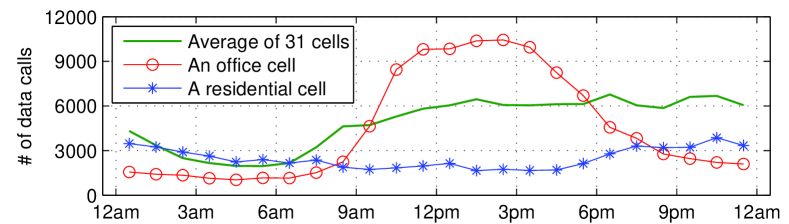
Figure 3: The number of data calls on average and in office/residential cells.

Trace 2 (WiFi connection). The second trace is measured by 93 iPhone users from an iPhone user community in Korea, who volunteer and record their time-varying WiFi connectivity and locations, periodically scanned and recorded at every 3 minutes for two weeks [4]. Occupations of participants were diverse, e.g. students, daytime workers, and freelancers, as well as residential areas were, where half of participants lived in Seoul. We only recorded APs to which users can transmit data by sending a ping packet to our server. i.e., the trace only captures accessible WiFi APs that are open or users have authority.

We now present the main parameters based on the traces 1, 2 and the measurement results revealed in other research.

(a) Traffic demand (${\phi}_{i}$) and willingness to pay ($\gamma_{i}(t)$): Most measurements on mobile data [18, 13, 19, 14] showed that the user traffic volume follows an upper-truncated power-law distribution as used in the analysis of Section IV. Thus, we use an upper-truncated power-law distribution with exponent $\sigma=0.57$ (which is observed in [14]), as the distribution of total daily traffic demand ${\Phi}_{i}$ by scaling the average, so that the per-month average ranges from 93 MB to 5.2 GB. Note that in [1], 1.3 GB/month is projected in year 2015. The temporal preference ($w_{i}(t)=\phi_{i}(t)/\Phi_{i}$) of users follows the average temporal usage pattern in trace 1. Users’ willingness to pay is set to include some randomness across users, and its time-dependence is set to be proportional to temporal preference, i.e., $\gamma_{i}(t)=\nu_{i}w(t)^{1-\theta},$ where $\nu_{i}$ is uniformly distributed over $(0,1).$

(b) WiFi connection probability ($e_{i}^{d}(t)$): We use the trace 2 to obtain the values of $(e_{i}^{d}(t):i\in N,t\in T).$ Since trace 2 includes only 93 users, we repeatedly use their individual traces to generate $N$ users’ data, i.e., about $N/93$ users have the same $e_{i}^{d}(t).$ We refer the readers to [4] to know how often users meet WiFi in the experiment. For 10 mins and 6 hours deadline, the average WiFi contact probabilities are 0.7 and 0.88, and the medians are 0.87 and 0.97, resp.

(c) BS association ($s_{i}(t)$): The information on cell-level mobility is important in our model due to the (i) cell-level capacity constraint $C_{\text{3g}}$ (which requires to track the number of users in a cell) and (ii) congestion pricing (which applies difference prices depending on spatio-temporal information). Unfortunately, trace 1 does not include users’ cell-level mobility mainly because of privacy, thus we combine trace 1 with the statistics from [13] that has the distribution on the number of distinct BSs visited by a user per day. At the first time slot, we assign user associations so that the number of users in each cell at the first time slot is proportional to the traffic volume of the cell at that slot (e.g. 8 a.m.) in trace 1. We assign handover probabilities (from the associated cell to other cells) to users so that (i) the expected number of users in each cell at the next time slot is proportional to the traffic volume in trace 1 and (ii) the number of visited BSs follows the statistics in [13], assuming that handovers are uniformly distributed among time slots.

(d) Delay profile ($\alpha_{i}^{d}$): To model the delay profile of users, we use various scenarios, such as no-deadline, short, medium, and long, where each scenario consists of four different classes (Video, Data, P2P, and Audio), as classified by Cisco [1]. The details are described in Table II. We consider the economic impact of WiFi offloading for two cases in our numerical results: (i) all users are uniformly given a scenario, e.g., medium, and (ii) there is a fixed portion of users for each scenario.

TABLE II: Traffic classification projected in year 2015 from Cisco [1] and assigned deadlines for each traffic class. SC: Scenario

	Video	Data	P2P	Audio (VoIP)	Total
Ratio	66.4 %	20.9 %	6.1 %	6.6 %	100 %
SC:zero	0 sec.	0 sec.	0 sec.	0 sec.	-
SC:short	10 min.	30 min.	10 min.	0 sec.	-
SC:medium	30 min.	1 hour	30 min.	0 sec.	-
SC:long	2 hours	6 hours	2 hours	0 sec.	-

V-B Results

Our numerical results quantify the benefits of delayed WiFi offloading in various aspects. We present our results by summarizing the key observations.

1) Revenue in volume pricing exceeds that in flat pricing by applying delayed WiFi offloading, but the revenue increase is higher in flat pricing than volume pricing: Fig. 4(a) depicts the revenue of flat and volume for various traffic demand and delay profiles, where users experience a single scenario. Revenue in volume exceeds that in flat in all cases, because in flat, a subscriber with high traffic demand generates heavy traffic and dominates the network resources without paying more fees to the provider, whereas in volume, user payment is proportional to traffic volume, so that if a subscriber generates heavy traffic, the payment is high. This imposes negative externality (i.e., congestion) to the provider and reduces provider revenue. However, the revenue increase of delayed offloading, which is the amount of increased revenue over revenue in the on-the-spot offloading, is higher in flat. The revenue increase in flat pricing is about 61-152%, whereas the revenue increase in volume pricing is about 21-43%, when the average traffic demand is 43.3 MB/day (1.5 GB/month). This is because in flat pricing, 3G traffic reduction does not affect the provider’s income, whereas, in volume pricing, 3G traffic reduction decreases the income. We also depict the revenue of flat and volume pricing when users have a mixture of four scenarios of delay deadline in Fig. 5. We find that as user portion with high delay tolerance increases, revenue increases in both flat and volume pricing.

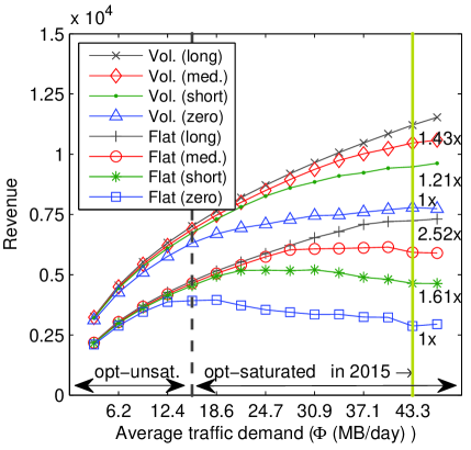
(a) $C_{\text{3g}}$ = 3.6 GB/hour (8 Mbps)

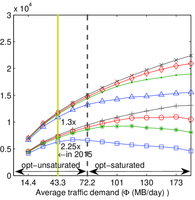
(b) $C_{\text{3g}}$ = 14.4 GB/hour (32 Mbps)

Figure 4: Flat and volume pricing: revenue for various delay profiles in Table II and traffic demand, with different cellular capacities, where users experience a single scenario in Table II. Delay profiles are set to be the same across all users. Offloading indicators are decreasing as delay tolerance gets higher (from short to long), where $\kappa_{\text{avg}}=.44,~{}.28,~{}.23,~{}.15$ and $\kappa_{\text{peak}}=.0044,~{}.0026,~{}.0020,~{}.0013$ for zero, short, medium, and long scenarios. The numbers (-x) represent the increase of revenue by (a) delayed offloading or (b) network upgrade (from 3G to 4G). Opt-saturatedness and opt-unsaturatedness are determined by the traffic demand and cellular capacity, where the dotted line shows the threshold in the on-the-spot offloading over flat pricing.

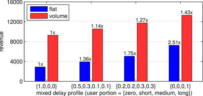
Figure 5: Revenue in flat and volume pricing with various mixed delay profiles, where user portions of scenarios (zero, short, medium, long) are different. The average traffic demand is 43.3 MB/day (1.5 GB/month) and 3G capacity is 3.6 GB/hour. The numbers (-x) represent the increase of revenue compared to the revenue in on-the-spot offloading.

2) The revenue gain from on-the-spot to delayed offloading is similar to that generated by the network upgrade from 3G to 4G: Fig. 4 depicts revenue of flat and volume pricing for various traffic demand, with different cellular capacities. As the traffic demand increases, the network gets congested and eventually becomes opt-saturated. If a provider upgrades the cellular network, such as a 4G network, the revenue increases by 115% in flat and 30% in volume, respectively, when the traffic demand is 43.3 MB/day. We recall that the revenue gain of offloading in flat and volume pricing is 61-152% and 21-43%, which is as significant as the revenue gain from network upgrade from 3G to 4G. Thus, if traffic demand is high compared to capacity, adopting delayed offloading can be a good solution to increase revenue, where the network upgrade induces huge installation costs. Note that when traffic demand is not high (i.e., opt-unsaturated), the revenue increase is small both in network upgrade and delayed offloading.

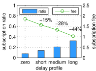
(a) Flat: fee and subscription ratio

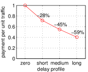
(b) Volume: payment per unit traffic

Figure 6: Change of flat price and subscription ratio in flat pricing, and payment per unit traffic in volume pricing. The average traffic demand is 43.3 MB/day (1.5GB/month) and 3G capacity is 3.6 GB/hour (opt-saturated).

3) As more traffic is offloaded, the flat price decreases and subscription ratio increases simultaneously in flat pricing, and payment per unit traffic decreases in volume pricing: As shown in Fig. 6, the flat fee decreases by 15-44% and subscription ratio increases accordingly in flat pricing, and payment per unit traffic decreases by 28-59% in volume pricing, when the average traffic demand is 1.5 GB/month (opt-saturated). In the opt-unsaturated case, price reduction is not drastic both in flat and volume pricing, since the income does not increase by price reduction due to low traffic demand. The reduction in flat price and payment per unit traffic induces increase in user surplus, as shown in Fig. 7.

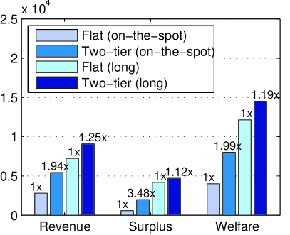
(a) Flat vs. Two-tier

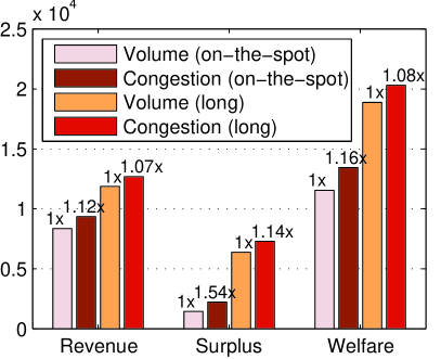
(b) Volume vs. Congestion

Figure 7: The revenue, surplus, and welfare in flat, tiered, volume and congestion pricing. The number (-x) above each bar represents the increase compared to the revenue in (a) flat or (b) volume pricing. The average traffic demand is set to be 43.3MB/day (1.5GB/month) which is projected in year 2015 by Cisco and the 3G capacity is 3.6GB/hour.

4) Two-tier and congestion pricing increase the revenue, compared to flat and volume pricing, but such gains become smaller, as more traffic is offloaded: Fig. 7 shows the change of revenue, surplus, and welfare in four pricing schemes. It is intuitive that as pricing granularity increases in terms of price (from flat to tiered) or space/time (from volume to congestion), revenue increases, because the provider has more degree of freedom to control the market. However, the rate of increase diminishes as more traffic is offloaded through WiFi. Using the traffic demand in 2015, the revenue in two-tier pricing is greater than that in flat pricing by 94% and 25% in on-the-spot and delayed offloading, resp., where the revenue in congestion pricing is greater than that in volume pricing by 12% and 7% in on-the-spot and delayed offloading, resp. We also find that delayed offloading reduces spatiotemporal imbalance by dispersing traffic to other time and locations, so that the effect of space/time-varying price is reduced. To see this, we depict the variance of normalized cell load at each time in Fig. 8, where the variance decreases as more traffic is offloaded. As a result, the time-flattening effect and revenue increase of congestion pricing decrease, since congestion pricing performs better when temporal imbalance in traffic demand is severe.

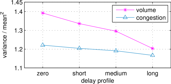
Figure 8: Variance of normalized cell load at each time slot.

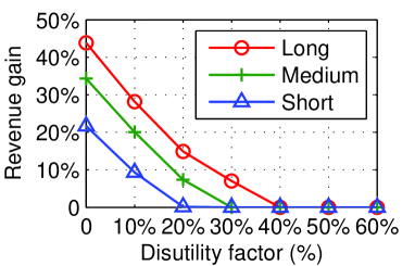
(a) Decrease in the revenue gain.

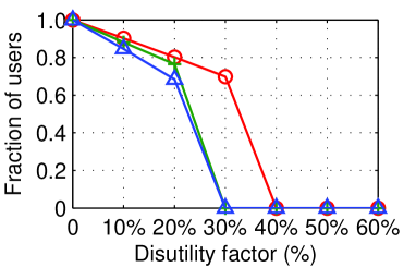
(b) Decrease in the fraction of delayed offloading users.

Figure 9: Effect of delay disutility on (a) the revenue gain and (b) the fraction of delayed offloading users

5) As users’ utility decreases by the delay disutility, the revenue gain from delayed offloading decreases, but the decrease in revenue gain is not severe when users have high delay tolerance: Here, we try to understand the effect of delay disutility on revenue gain by applying the disutility factor in users’ utility. We consider the volume pricing and assume that utility of users who perform delayed offloading is decreased by the disutility factor (%) from the original utility without delayed offloading. A user can decide whether it adopts delayed offloading or not, based on the net-utility, i.e., only if the price discount is higher than the amount of disutility, the user adopts delayed offloading. We depict the revenue gain and the fraction of users who adopt delayed offloading, in Fig. 9. Both the revenue gain and the delayed offloading ratio decrease as the disutility factor increases. We still obtain more than 50% of the revenue gain when users have less than 15% and 10% of disutility factor, for the long and short delay profiles, resp. Note that users will experience less delay disutilty for shorter delay. When the disutility factor is higher than 40%, no user decides to use delayed offloading, so that the revenue gain is zero.

VI Concluding Remark and Future Work

In this paper, we model a game-theoretic framework to study the economic aspects of WiFi offloading, where we drew the following messages from the analytical and numerical studies: First, WiFi offloading is economically beneficial for both a monopoly provider and users, where the economic gains are not ignorable. Also, a simple pricing is enough in the sense that two-tier and volume-based pricing do not increase the revenue and the net-utilities for higher offloading chances, which is true as of now and in the future, when more WiFi APs are expected to be deployed.

Another well-known benefit from WiFi offloading is Smartphone energy reduction, which is shown in [20, 4, 21]. This is mainly because short range communication (e.g. WiFi) typically has lower energy-per-bit than long range communication (e.g. 3G/4G). It is shown that 50-60% of transmission energy can be reduced for 1-hour delay [4]. Even though we do not consider the energy benefit in this paper, it is obvious that most users benefit from the increased battery lifetime.

There are a few limitations in our work. Our results rely on the assumption that network traffic has a degree of delay tolerance and users can tolerate some amount of delay, where delay depends on the class of traffic (even if we provide the numerical results of a mixture of users with different delay scenarios, including ones requiring no delay deadline). Thus, our results can sometimes be regarded as an upper-bound on the economic benefits of WiFi offloading. A simple way of reflecting those limitations would be to design a net-utility function which jointly captures the happiness by data transmission and the disutility by delay, which we leave as a future work. Another future work is to consider multiple providers, where they have different plans to overcome the mobile data explosion (e.g. delayed offloading, network upgrade, and complex pricing).

VII Appendix

VII-A Proof of Proposition IV.1

Step 1: Unimodality of $R(p)$. In flat pricing, the total 3G traffic volume of a 3G-subscribing user is equal to its total traffic demand, i.e., $\sum_{t\in T}x_{\Phi}(t)=\sum_{t\in T}\phi(t)=\Phi,$ and the user enters the market only when $\Phi>p^{\frac{1}{\theta}},$ from (7). Based on it, we first express $\sum_{x\in T}X(t)$ and $A(p)$ using the parameters of the traffic demand distribution. We first have:

$$\sum_{t\in T}X(t)=\hat{N}\int_{p^{\frac{1}{\theta}}}^{{\Phi}_{\max}}{\Phi}f_{\Phi}({\Phi})d\Phi=\hat{N}\frac{{\Phi}_{\max}^{2-\sigma}-p^{\frac{2-\sigma}{\theta}}}{Z(2-\sigma)},$$

where $f_{\Phi}({\Phi})=\frac{{\Phi}^{-\sigma}}{Z}$ by A2 and recall that $Z=\frac{{\Phi}_{\max}^{1-\sigma}}{1-\sigma}.$ Then, by (4),

$$A(p)=\kappa_{\text{peak}}\sum_{t\in T}X(t)=\kappa_{\text{peak}}\hat{N}\frac{{\Phi}_{\max}^{2-\sigma}-p^{\frac{2-\sigma}{\theta}}}{Z(2-\sigma)}.$$ (12)

From (8), the revenue $R(p)$ is expressed as:

$$R(p) = \hat{N}p\left(1-\frac{p^{\frac{1-\sigma}{\theta}}}{Z(1-\sigma)}\right)-\frac{\eta\kappa_{\text{avg}}\hat{N}\left({\Phi}_{\max}^{2-\sigma}-p^{\frac{2-\sigma}{\theta}}\right)}{Z(2-\sigma)}.$$

Then, the first derivative of $R(p)$ is

$$\frac{\partial R(p)}{\partial p}=\hat{N}\left(1-\frac{\left(1+\frac{1-\sigma}{\theta}\right)p^{\frac{1-\sigma}{\theta}}}{Z(1-\sigma)}+\frac{\eta\kappa_{\text{avg}}p^{\frac{2-\sigma}{\theta}-1}}{Z\theta}\right).$$ (13)

We can easily check that $R^{\prime}(0)>0$ and $R^{\prime}(p_{\max})<0$ under the condition that $\eta<(\kappa_{\text{avg}}{\Phi}_{\max}^{1-\theta})^{-1}$. and from the intermediate value theorem, there exists a price $\hat{p}\in(0,p_{\max})$ such that $R^{\prime}(\hat{p})=0.$ Now, we show that $R(p)$ is unimodal, thereby $\hat{p}$ is unique. The second derivative of $R(p)$ is

$$\frac{\partial^{2}R(p)}{{\partial p}^{2}}=\hat{N}p^{\frac{1-\sigma-\theta}{\theta}}\frac{\eta\kappa_{\text{avg}}p^{\frac{1-\theta}{\theta}}(2-\theta-\sigma)-(1+\theta-\sigma)}{Z\theta^{2}}.$$ (14)

We have ${\partial^{2}R(p)}/{{\partial p}^{2}}<0$ (concave) over $[0,\bar{p}),$ and ${\partial^{2}R(p)}/{{\partial p}^{2}}>0$ (convex) over $(\bar{p},p_{\max}),$ where $\bar{p}=\left(\frac{1+\theta-\sigma}{\eta\kappa_{\text{avg}}(2-\theta-\sigma)}\right)^{\frac{\theta}{1-\theta}},$ such that ${\partial^{2}R(p)}/{{\partial p}^{2}}=0.$ Since $R^{\prime}(p_{\max})<0$ and $R^{\prime}(p)$ is increasing over $(\bar{p},p_{\max})$ from the convexity, $R^{\prime}(p)<0$ over $(\bar{p},p_{\max}),$ and $R^{\prime}(\bar{p})<0.$ Thus, $\hat{p}\notin[\bar{p},p_{\max}).$ Since $R^{\prime}(0)>0,$ $R^{\prime}(\bar{p})<0,$ and $R^{\prime}(p)$ is decreasing over $[0,\bar{p})$ from the concavity, the solution of $R^{\prime}(\hat{p})=0,$ $\hat{p}$ is unique and $\hat{p}<\bar{p}.$ Also, $R(p)$ is unimodal over $[0,p_{\max})$ since $R^{\prime}(p)$ has only one sign change.

Step 2: Characterization of $\mathcal{P}$. By definition of the set of feasible prices with provider rationality and capacity constraint, $\mathcal{P}=\mathcal{E}\cap\mathcal{F}$ where $\mathcal{E}=\{p~{}|~{}A(p)\leq C_{3g}\}$ and $\mathcal{F}=\{p~{}|~{}R(p)>0\}$. From (12), $A(p)$ is decreasing in $p.$ Thus, there exists some $p_{\min},$ such that $A(p)\leq C_{3g}\Leftrightarrow p\geq p_{\min}.$ Therefore, $\mathcal{E}=\{p~{}|~{}p\geq p_{\min}\}$ which is a connected set. The $p_{\min}$ is characterized as:

$$p_{\min}=\left\{\begin{array}[]{ll}0&\mbox{if $A(0)<C_{\text{3g}}$}\\ \left({\Phi}_{\max}^{2-\sigma}-\frac{C_{3g}Z(2-\sigma)}{\hat{N}\kappa_{\text{peak}}}\right)^{\frac{\theta}{2-\sigma}}&\mbox{if $A(0)\geq C_{\text{3g}}$}\end{array}\right.$$

Note that $p_{\min}<\Phi^{\theta}_{\max}$ since $0<\sigma<1.$ Regarding $\mathcal{F}$, we first recall that $p<p_{\max}=\Phi_{\max}^{\theta}$ since $R(p)=0$ for $p\geq{\Phi}^{\theta}_{\max}$ (i.e., there exists no subscriber). Since $R(p)$ is unimodal over $[0,p_{\max}),$ $\mathcal{F}=\{p~{}|~{}R(p)>0\}$ is connected. There exists a unique $p_{z}<\hat{p}$ such that $R(p_{z})=0,$ since $R(0)\leq 0,~{}R(\hat{p})>0$ and $R(p)$ is strictly increasing ($R^{\prime}(p)>0$) in $0\leq p\leq\hat{p}.$ Hence $\mathcal{F}=(p_{z},~{}p_{\max})$ for $p_{z}<p_{\max}$ such that $R(p_{z})=0.$ Since both $\mathcal{E}$ and $\mathcal{F}$ are connected, $\mathcal{P}=\mathcal{E}\cap\mathcal{F}$ is connected. Note that $p_{0}=\inf\{p|R(p)>0,A(p)\leq C_{\text{3g}}\}=\max\{p_{\min},p_{z}\}.$ If $R(p_{0})>0$, $p_{0}\in\mathcal{F}$ and $\mathcal{P}=[p_{0},~{}p_{\max}).$ If $R(p_{0})=0,$ then, $p_{0}\notin\mathcal{F}$. Thus, $p_{0}=p_{z}$ and $\mathcal{P}=(p_{0},~{}p_{\max}).$ From Steps 1 and 2, the result (i) holds.

Step 3: Proof of (ii). If $R^{\prime}(p_{0})<0$, then $\hat{p}<p_{0},$ which means $\hat{p}$ is not in $\mathcal{P}$, i.e, $\hat{p}$ cannot be the equilibrium price. Since $R(p_{\max})=0$ and $R^{\prime}(p)<0$ for $p_{0}\leq p\leq p_{\max}$ from unimodality of $R(p)$ we have $R(p_{0})>0$; $\mathcal{P}=[p_{0}~{}p_{\max}).$ Therefore $p_{0}=p_{\min}$ such that $A(p_{\min})=C_{\text{3g}}$ and

$$p_{0} = \left({\Phi}_{\max}^{2-\sigma}-\frac{C_{3g}Z(2-\sigma)}{\kappa_{\text{peak}}\hat{N}}\right)^{\frac{\theta}{2-\sigma}}$$

$$= {\Phi}_{\max}^{\theta}\left(1-\frac{C_{3g}}{\kappa_{\text{peak}}\hat{N}\mathbb{E}[{\Phi}]}\right)^{\frac{\theta}{2-\sigma}},$$

where $\mathbb{E}[\Phi]=\frac{1-\sigma}{2-\sigma}\Phi_{\max}.$ Since $R(p)$ is decreasing over $\mathcal{P}$, $R(p)$ is maximum at $p_{0}$, that is, $p_{0}$ is the unique equilibrium price. Since $A(p_{0})=C_{\text{3g}}$, the network is opt-saturated.

Step 4: Proof of (iii). If $R^{\prime}(p_{0})>0$, then $\hat{p}>p_{0}$ since $R(p)$ is unimodal. From (12), $A(p)$ is a decreasing function of $p$. Hence $A(\hat{p})<A(p_{0})\leq C_{3g}$; the network is opt-unsaturated. We will show that the derivative $\frac{\partial\hat{p}}{\partial\kappa_{\text{avg}}}$ is positive. From (13) and taking a derivative of $\kappa_{\text{avg}}$ w.r.t. $\hat{p},$

$$\kappa_{\text{avg}}=\frac{\frac{1+\theta-\sigma}{1-\sigma}\hat{p}^{\frac{1-\sigma}{\theta}}-Z\theta}{\eta\hat{p}^{\frac{2-\sigma}{\theta}-1}},\quad\frac{\partial\kappa_{\text{avg}}}{\partial\hat{p}}=\frac{\hat{p}^{\frac{-2+\sigma}{\theta}}}{\eta(1-\sigma)}g(\hat{p}^{\frac{1-\sigma}{\theta}}),$$

where $g(z)=(2-\theta-\sigma){\Phi}_{\max}^{1-\sigma}-\frac{(1-\theta)(1+\theta-\sigma)}{\theta}z.$ To show $\frac{\partial\hat{p}}{\partial\kappa_{\text{avg}}}>0$, it suffices to show $\frac{\partial\kappa_{\text{avg}}}{\partial\hat{p}}>0$, for which we show $g(\hat{p}^{\frac{1-\sigma}{\theta}})>0$. From (13), we have

$$\hat{p}^{\frac{1-\sigma}{\theta}} = \frac{\theta{\Phi}_{\max}^{1-\sigma}}{(1+\theta-\sigma)-\eta\kappa_{\text{avg}}(1-\sigma)\hat{p}^{\frac{1-\theta}{\theta}}}$$

$$< \frac{\theta{\Phi}_{\max}^{1-\sigma}}{(1+\theta-\sigma)\left(1-\frac{1-\sigma}{2-\theta-\sigma}\right)}$$

$$= \frac{\theta(2-\theta-\sigma)}{(1-\theta)(1+\theta-\sigma)}{\Phi}_{\max}^{1-\sigma},$$

since $\hat{p}<\bar{p},$ where $\bar{p}=\left(\frac{1+\theta-\sigma}{\eta\kappa_{\text{avg}}(2-\theta-\sigma)}\right)^{\frac{\theta}{1-\theta}}$ such that ${\partial^{2}R(p)}/{{\partial p}^{2}}=0$ from (14). Let $\rho=\frac{\theta(2-\theta-\sigma)}{(1-\theta)(1+\theta-\sigma)}{\Phi}_{\max}^{1-\sigma}$. Since $g(z)$ is decreasing as $z$ is increasing and $g(\rho)=0$, $g(\hat{p}^{\frac{1-\sigma}{\theta}})>g(\rho)=0$ since $\theta\in(0,1)$ and $\sigma\in(0,1).$ Thus, $\frac{\partial\kappa_{\text{avg}}}{\partial\hat{p}}>0$ and $\frac{\partial\hat{p}}{\partial\kappa_{\text{avg}}}$ is also positive. ∎

Figure 10: Change of feasible price set, $\mathcal{P}=E\cap F$ for $\kappa_{\text{avg}}=1,~{}\kappa_{\text{peak}}=1$ and $\kappa_{\text{avg}}=0.5,~{}\kappa_{\text{peak}}=0.5$ in flat pricing.

VII-B Proof of Theorem IV.1

(i) Opt-saturated. Recall that net-utility of a subscriber with ${\Phi}$ is ${\Phi}^{\theta}-p,$ where ${\Phi}=\sum_{t\in T}{\phi}(t).$ Hence, the net-utility of a subscriber increases as $p^{\star}$ decreases from Proposition IV.1(ii).

To study the impact of $\kappa_{\text{peak}}$, we regard $\kappa_{\text{peak}}$ as a variable, not a constant. To show that $R(p^{\star})$ increases as $\kappa_{\text{peak}}$ decreases, we will show that $\frac{\partial R(p^{\star})}{\partial\kappa_{\text{peak}}}<0$. The first derivative of $R(p^{\star})$ with respect to $\kappa_{\text{peak}}$ is,

$$\frac{\partial R(p^{\star})}{\partial\kappa_{\text{peak}}}=\frac{\partial R(p^{\star})}{\partial p^{\star}}\frac{\partial p^{\star}}{\partial\kappa_{\text{peak}}}.$$

From Proposition IV.1(ii), $p^{\star}$ is an increasing function in $\kappa_{\text{peak}}$. Therefore, it suffices to show that $\frac{\partial R(p^{\star})}{\partial p^{\star}}<0$, which is proved in the proof of Proposition IV.1(ii).

(ii) Opt-unsaturated. Using a similar argument in the proof of Theorem IV.1(i), the net-utility of a user and user surplus increase as $\kappa_{\text{avg}}$ decreases, since the flat fee decreases as $\kappa_{\text{avg}}$ decreases from Proposition IV.1(iii). In terms of the provider’s revenue, we use the notations $R(p,\kappa_{\text{avg}})$ and $\mathcal{P}_{\kappa_{\text{avg}}}$ to explicitly express the dependence of $R(p)$ and $\mathcal{P}$ on $\kappa_{\text{avg}},$ because our interest lies in examining how $R(p)$ and $\mathcal{P}$ change with varying $\kappa_{\text{avg}}.$ First, $R(p,\kappa_{\text{avg}})$ increases as $\kappa_{\text{avg}}$ decreases for $p\in[0,p_{\max}],$ since differentiating by $\kappa_{\text{avg}}$ yields:

$$\frac{\partial R(p,\kappa_{\text{avg}})}{\partial\kappa_{\text{avg}}}=-\frac{\eta\hat{N}\left(\Phi_{\max}^{2-\sigma}-p^{\frac{2-\sigma}{\theta}}\right)}{Z(2-\sigma)}<0.$$ (16)

Second, we will show that the set $\mathcal{P}_{\kappa_{\text{avg}}}$ gets “enlarged” as $\kappa_{\text{avg}}$ decreases, for which it suffices to show that revenue increases. $\mathcal{P}_{\kappa_{\text{avg}}}=\mathcal{E}\cap\mathcal{F}_{\kappa_{\text{avg}}},$ where $\mathcal{E}=\{p~{}|~{}p\geq p_{\min}\}$ and $\mathcal{F}_{\kappa_{\text{avg}}}=\{p~{}|~{}R(p,\kappa_{\text{avg}})>0\}.$ Note that $\mathcal{E}$ does not depend on $\kappa_{\text{avg}},$ but on $\kappa_{\text{peak}}.$ Since $R(p,\kappa_{\text{avg}})$ is decreasing in $\kappa_{\text{avg}}$, $\mathcal{F}_{\kappa_{\text{avg}}}$ is enlarged as $\kappa_{\text{avg}}$ decreases. Therefore, $\mathcal{P}_{\kappa_{\text{avg}}}$ is enlarged (or remains the same) and $\max_{p\in\mathcal{P}_{\kappa_{\text{avg}}}}R(p,\kappa_{\text{avg}})$ increases as $\kappa_{\text{avg}}$ decreases. We illustrate this in Fig. 10. ∎

VII-C Proof of Proposition IV.2

Step 1: Unimodality of $R(p)$. From (10),

$${U}(\bm{x}_{\Phi})=\sum_{t\in{T}}\left(w(t)^{1-\theta}x_{\Phi}(t)^{\theta}-p\kappa_{\text{avg}}x_{\Phi}(t)\right).$$ (17)

Let $v(x_{\Phi}(t))=w(t)^{1-\theta}x_{\Phi}(t)^{\theta}-p\kappa_{\text{avg}}x_{\Phi}(t)$. The net-utility ${U}(\bm{x}_{\Phi})$ is maximized when $v(x_{\Phi}(t))$ is maximized for each $t$. At given $t$,

$$\frac{\partial v(x_{\Phi}(t))}{\partial x_{\Phi}(t)}=\theta w(t)^{1-\theta}x_{\Phi}(t)^{\theta-1}-p\kappa_{\text{avg}},$$

$$\frac{\partial^{2}v(x_{\Phi}(t))}{{\partial x_{\Phi}(t)}^{2}}=-\theta(1-\theta)w(t)^{1-\theta}x_{\Phi}(t)^{\theta-2}.$$

Since $\theta\in(0,1),$ $\frac{\partial^{2}v(x_{\Phi}(t))}{{\partial x_{\Phi}(t)}^{2}}<0$. Therefore, $v(x(t))$ is concave in $x(t)$. Thus, at each time $t$, $v(x_{{\Phi}}(t))$ takes a unique maximum at

$${x}_{{\Phi}}^{\star}(t) = \min\left\{{\phi}(t),w(t)\left(\frac{\theta}{p\kappa_{\text{avg}}}\right)^{\frac{1}{1-\theta}}\right\}$$

$$= w(t)\min\left\{\Phi,\left(\frac{\theta}{p\kappa_{\text{avg}}}\right)^{\frac{1}{1-\theta}}\right\}.$$

The second equality holds since $\phi(t)=w(t)\Phi$ and $\Phi=\sum_{t\in{T}}\phi(t).$ Moreover, it can be easily shown that $v(x^{\star}_{{\Phi}}(t))>0$ for all $t$. This implies that a user with positive $\Phi$ subscribes the service and $x_{\Phi}^{\star}(t)\neq 0$. Therefore,

$$\sum_{t\in{T}}{x}_{{\Phi}}^{\star}(t)=\left\{\begin{array}[]{ll}\Phi&\mbox{ if $\Phi<\left(\frac{\theta}{p\kappa_{\text{avg}}}\right)^{\frac{1}{1-\theta}}$}\\ \Psi(p)&\mbox{ if $\Phi>\left(\frac{\theta}{p\kappa_{\text{avg}}}\right)^{\frac{1}{1-\theta}}$}\end{array}\right.$$

where $\Psi(p)=\left(\frac{\theta}{p\kappa_{\text{avg}}}\right)^{\frac{1}{1-\theta}}.$ Then, total user traffic over a day, $\sum_{t\in{T}}X(t)$ is as follows:

$$\sum_{t\in{T}}X(t)=\hat{N}\int_{0}^{\Phi_{\max}}\sum_{t\in{T}}x^{\star}_{\phi}(t)f_{\Phi}({\Phi})d\Phi$$

$$= \hat{N}\left(\int_{0}^{\Psi(p)}{\Phi}f_{\Phi}({\Phi})d\Phi+\int_{\Psi(p)}^{{\Phi}_{\max}}\Psi(p)f_{\Phi}({\Phi})d\Phi\right)$$

$$= \left\{\begin{array}[]{ll}\hat{N}\Psi(p)\left(1-\frac{\Psi(p)^{1-\sigma}}{(2-\sigma)\Phi_{\max}^{1-\sigma}}\right)&\mbox{ if $\Psi(p)\leq\Phi_{\max}.$ }\\ \hat{N}\mathbb{E}[\Phi]&\mbox{ if $\Psi(p)>\Phi_{\max}.$}\end{array}\right.$$

We denote

$$B(p) = \sum_{t\in{T}}Y(t;p)=\kappa_{\text{avg}}\sum_{t\in{T}}X(t;p)$$

$$A(p) = \max_{t\in{T}}Y(t;p)=\kappa_{\text{peak}}\sum_{t\in{T}}X(t;p).$$ (20)

By (11), the revenue of the provider is $R(p)=(p-\eta)B(p).$

We now show that $R(p)$ is unimodal over $\mathcal{P}.$ Note that

$$\Psi(p)>{\Phi}_{\max}~{}~{}\Leftrightarrow~{}~{}p<\theta\big{(}\kappa_{\text{avg}}{\Phi}_{\max}^{1-\theta}\big{)}^{-1}.$$

If $p<\theta\big{(}\kappa_{\text{avg}}{\Phi}_{\max}^{1-\theta}\big{)}^{-1}$ , then $B(p)$ is a positive constant, $B(p)=\kappa_{\text{avg}}\hat{N}\mathbb{E}[\Phi]$, for all $p\in\mathcal{P}$ and $\frac{\partial R(p)}{\partial p}=\kappa_{\text{avg}}\hat{N}\mathbb{E}[\Phi]$. We now consider the case

$$p\geq\theta\big{(}\kappa_{\text{avg}}{\Phi}_{\max}^{1-\theta}\big{)}^{-1}~{}~{}\Leftrightarrow~{}~{}\Psi(p)\leq{\Phi}_{\max}.$$

Then for $p\geq\theta\big{(}q{\Phi}_{\max}^{1-\theta}\big{)}^{-1},$

$$B(p)=\hat{N}\kappa_{\text{avg}}\Psi(p)\left(1-\frac{\Psi(p)^{1-\sigma}}{(2-\sigma)\Phi_{\max}^{1-\sigma}}\right)>0,$$

since $B(p)>0$, $sgn(R^{\prime}(p))=sgn{\left(\frac{R^{\prime}(p)}{B(p)}\right)}$. We will investigate $sgn(R^{\prime}(p))$ by investigating $sgn{\left(\frac{R^{\prime}(p)}{B(p)}\right)}$ and show that $\frac{\partial R(p)}{\partial p}$ has a unique solution $\hat{p}$ of $\frac{\partial R(p)}{\partial p}=0$ by showing that ${\frac{R^{\prime}(p)}{B(p)}}=0$ has a unique solution at $\hat{p}$. The first and second derivatives of $B(p)$ are,

$$\frac{\partial B(p)}{\partial p} = \frac{-\hat{N}\kappa_{\text{avg}}\Psi(p)}{p(1-\theta)}\left(1-\frac{\Psi(p)^{1-\sigma}}{\Phi_{\max}^{1-\sigma}}\right),$$

$$\frac{\partial B(p)^{2}}{\partial^{2}p} = \frac{\hat{N}\kappa_{\text{avg}}\Psi(p)}{p^{2}(1-\theta)^{2}}\left((2-\theta)-\frac{(3-\sigma-\theta)\Psi(p)^{1-\sigma}}{\Phi_{\max}^{1-\sigma}}\right).$$

Let $B^{\prime}(p)=\frac{\partial B(p)}{\partial p}$ and $B^{\prime\prime}(p)=\frac{\partial B(p)^{2}}{\partial^{2}p}$. The first derivative of revenue function $R(p)$ is

$$\frac{\partial R(p)}{\partial p}=(p-\eta)B^{\prime}(p)+B(p).$$ (21)

We have

$$\frac{\partial\left(\frac{R^{\prime}(p)}{B(p)}\right)}{\partial p} = \frac{B^{\prime}(p)}{B(p)}+(p-\eta)\frac{B^{\prime\prime}(p)B(p)-B^{\prime}(p)^{2}}{B(p)^{2}}$$

$$= \frac{-l(p)}{p^{2}(1-\theta)^{2}B(p)^{2}}<0,$$

where

$$l(p) = (p-\eta)\left(\frac{(1-\sigma)^{2}\Psi(p)^{1-\sigma}}{(2-\sigma)\Phi_{\max}^{1-\sigma}}\right)+$$

$$~{}~{}~{}\eta(1-\theta)\left(1-\frac{\Psi(p)^{1-\sigma}}{\Phi_{\max}^{1-\sigma}}\right)B(p)$$

$$> 0.$$

since $p\geq\eta,~{}0\leq\Psi(p)\leq\Phi_{\max},~{}B(p)>0,$ and $\theta\in(0,1).$ Thus, $\frac{R^{\prime}(p)}{B(p)}$ is strictly decreasing in $p.$ Note that $\frac{R^{\prime}(\eta)}{B(\eta)}=1>0,$ and

$$\lim_{p\rightarrow\infty}\frac{R^{\prime}(p)}{B(p)} = 1+\lim_{p\rightarrow\infty}\frac{-\frac{p-\eta}{p(1-\theta)}\left(1-\frac{\Psi(p)^{1-\sigma}}{\Phi_{\max}^{1-\sigma}}\right)}{1-\frac{\Psi(p)^{1-\sigma}}{(2-\sigma)\Phi_{\max}^{1-\sigma}}}$$

$$= 1-\frac{1}{1-\theta}<0,$$

since $\lim_{p\rightarrow\infty}\Psi(p)=0$ and $\theta\in(0,1).$ Therefore $\frac{R^{\prime}(p)}{B(p}<0$ for sufficiently large $p$. Considering that $\frac{R^{\prime}(p)}{B(p)}$ is a decreasing function of $p$ and $\frac{R^{\prime}(\eta)}{B(\eta)}>0$, there should be a unique $\hat{p}\in(\eta,\infty)$ such that $\frac{R^{\prime}(p)}{B(p)}=0$ (note that $\hat{p}>\eta$). Since $B(p)>0$ for any $p$, $R^{\prime}(p)=0$ only at $\hat{p}$. Summarizing, the sign of $R^{\prime}(p)$ is

$$sgn(R^{\prime}(p)) = sgn{\left(\frac{R^{\prime}(p)}{B(p)}\right)}$$

$$= \left\{\begin{array}[]{ll}+&\mbox{if $\eta\leq p<\hat{p}$}\\ 0&\mbox{if $p=\hat{p}$}\\ -&\mbox{if $p>\hat{p}$}.\end{array}\right.$$

Thus, $R(p)$ is unimodal for $p>\eta.$

Step 2: Characterization of $\mathcal{P}$. We now find the set of feasible prices $\mathcal{P}$. Since $\sum_{t\in{T}}X(t)>0$ and $\kappa_{\text{avg}}\leq 1$, the provider’s revenue is negative if $p\leq\eta$ from (11). By the provider rationality, i.e., $R(p)>0$ for $p\in\mathcal{P},$

$$p\in\mathcal{P}\Rightarrow p>\eta.$$ (23)

$A(p)$ is nonincreasing in $p,$ since

$$\frac{\partial A(p)}{\partial p}=\left\{\begin{array}[]{ll}0&\mbox{ if $\Psi(p)>\Phi_{\max}$}\\ \frac{-\hat{N}k\Psi(p)}{p(1-\theta)}\left(1-\frac{\Psi(p)^{1-\sigma}}{\Phi_{\max}^{1-\sigma}}\right)&\mbox{ if $\Psi(p)\leq\Phi_{\max}$}\end{array}\right.$$

Thus, if $p\in\mathcal{P}$, then

$$A(p)\leq C_{3g} \Leftrightarrow p~{}\geq~{}p_{\min},$$

where $p_{\min}=\inf\{p~{}|~{}A(p)\leq C_{\text{3g}}\}.$ Note that $p_{0}=\max\{p_{\min},\eta\}.$ Thus, if $\eta\geq p_{\min},$ $p_{0}=\eta$ and $\mathcal{P}=(p_{0},\infty),$ and if $\eta<p_{\min}$, $p_{0}=p_{\min}$ and $\mathcal{P}=[p_{0},\infty).$ Note that $p_{\min}=0$ if and only if $\kappa_{\text{peak}}\hat{N}\mathbb{E}[\Phi]\leq C_{\text{3g}},$ since $A(0)=\kappa_{\text{peak}}\hat{N}\mathbb{E}[\Phi].$ From Steps 1 and 2, the result (i) holds.

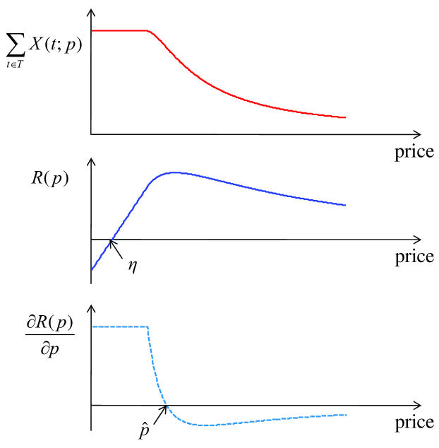
Figure 11: An illustration of $\sum_{t\in T}X(t;p),~{}R(p),$ and $\frac{\partial R(p)}{\partial p}$ over volume price $p.$

Step 3: Proof of (ii). If $R^{\prime}(p_{0})\leq 0,$ $\hat{p}\leq p_{0},$ $R(p_{0})>0$ and $p_{0}$ is the unique optimal price, since $R^{\prime}(p)\leq 0$ for $p\in\mathcal{P}.$ From $R(p_{0})>0,$ $p_{0}>\eta\geq 0.$ Thus, $A(p_{0})=C_{3g}$ and the network is opt-saturated.

We now show that $\frac{\partial p_{0}(\kappa_{\text{peak}})}{\partial\kappa_{\text{peak}}}>0.$ To study the impact of $\kappa_{\text{peak}}$, we regard $\kappa_{\text{peak}}$ as a variable, not a constant. Recall that $p^{\star}=p_{0}$ and $A(p_{0})=C_{\text{3g}}$ if the network is opt-saturated. From (4),

$$\kappa_{\text{peak}}=\frac{C_{\text{3g}}}{\sum_{t\in{T}}X(t;p_{0})},$$ (25)

where $X(t;p)$ is the total traffic arrival at time $t$ when price is $p.$ We denote $V(p)=\sum_{t\in{T}}X(t;p).$ Differentiating by $\kappa_{\text{peak}},$ we yield

$$\frac{\partial p_{0}}{\partial\kappa_{\text{peak}}} = \frac{-V(p_{0})^{2}}{C_{\text{3g}}V^{\prime}(p_{0})}>0,$$ (26)

where

$$\frac{\partial V(p)}{\partial p}=\left\{\begin{array}[]{ll}0&\mbox{ if $\Psi(p)>\Phi_{\max}$}\\ \frac{-\hat{N}\Psi(p)}{p(1-\theta)}\left(1-\frac{\Psi(p)^{1-\sigma}}{\Phi_{\max}^{1-\sigma}}\right)&\mbox{ if $\Psi(p)\leq\Phi_{\max}$}\end{array}\right.$$

since $V(p)>0$ and $V^{\prime}(p)<0,$ for $p\in\mathcal{P}$ in opt-saturated case. Note that $V^{\prime}(p)=0$ only if $\kappa_{\text{peak}}V(p)=\kappa_{\text{peak}}N\mathbb{E}[\Phi]>C_{\text{3g}}$ and $\kappa_{\text{peak}}V(p)\leq C_{\text{3g}}$ over $\mathcal{P}$ in opt-saturated case. By (26), the optimal price $p^{\star}$ decreases and actual payment per unit traffic $p^{\star}\kappa_{\text{avg}}$ decreases as $\kappa_{\text{peak}}$ decreases. We have proven (ii) holds.

Step 4: Proof of (iii). We now consider the case $R^{\prime}(p_{0})>0.$ If $\eta\geq p_{\min},$ then $\mathcal{P}=(\eta,\infty)$ and $\hat{p}>\eta$. Thus, $\hat{p}$ is the unique optimal price. To show that $A(\hat{p})<C_{\text{3g}},$ we consider two cases $p_{\min}=0$ and $p_{\min}>0.$ Recall that $p_{\min}=0$ if and only if $\kappa_{\text{peak}}\hat{N}\mathbb{E}[\Phi]\leq C_{\text{3g}},$ since $A(0)=\kappa_{\text{peak}}\hat{N}\mathbb{E}[\Phi].$ Thus, if $p_{\min}=0,$ $A(p_{\min})=\kappa_{\text{peak}}\hat{N}\mathbb{E}[\Phi]\leq C_{\text{3g}}.$ Note that $A^{\prime}(p)<0$ for $p$ such that $\Psi(p)\leq\Phi_{\max},$ i.e., $p\geq\theta\big{(}\kappa_{\text{avg}}\Phi_{\max}^{1-\theta}\big{)}.$ Since $\hat{p}\geq\theta\big{(}\kappa_{\text{avg}}\Phi_{\max}^{1-\theta}\big{)},$ $A^{\prime}(\hat{p})<0$ and $A(\hat{p})<A(p_{\min})\leq C_{\text{3g}}.$ If $p_{\min}>0,$ $A(p_{\min})=C_{\text{3g}}<\kappa_{\text{peak}}\hat{N}\mathbb{E}[\Phi].$ Since $A^{\prime}(\hat{p})<0,$ $A(\hat{p})<A(p_{0})\leq C_{\text{3g}}.$ The network is opt-unsaturated. If $\eta<p_{\min},$ then $p_{0}=p_{\min},$ $\mathcal{P}=[p_{\min},\infty)$ and $p_{\min}>0.$ Note that $A(p_{\min})=C_{\text{3g}}$ if $p_{\min}>0.$ Recall that if $R^{\prime}(p_{0})>0,$ then $\hat{p}>p_{0}$ and $\hat{p}$ is the unique optimal price. Since $A(\hat{p})<A(p_{\min})=C_{\text{3g}}$ (see Fig. 11), the network is opt-unsaturated.

We now show that $\frac{\partial(\hat{p}(\kappa_{\text{avg}})\kappa_{\text{avg}})}{\partial\kappa_{\text{avg}}}>0$ so that the optimal per-traffic payment is reduced as $\kappa_{\text{avg}}$ decreases. We use $\hat{p}(\kappa_{\text{avg}})$ to emphasize the impact of $\kappa_{\text{avg}}.$ From (21) and the condition $R^{\prime}(\hat{p}(\kappa_{\text{avg}}))=0,$

$$\hat{p}(\kappa_{\text{avg}})-\eta = -\frac{B(\hat{p})}{B^{\prime}(\hat{p})}$$

$$= \frac{\hat{p}(1-\theta)\left(1-\frac{h(\kappa_{\text{avg}})}{2-\sigma}\right)}{1-h(\kappa_{\text{avg}})},$$

where $h(\kappa_{\text{avg}})=\frac{\left(\frac{\theta}{\hat{p}(\kappa_{\text{avg}})\kappa_{\text{avg}}}\right)^{\frac{1-\sigma}{1-\theta}}}{\bar{\Phi}_{\max}^{1-\sigma}}>0.$ Differentiating by $\hat{p}$ and rearranging it, the derivative $\frac{\partial\hat{p}}{\partial\kappa_{\text{avg}}}$ is as follows:

$$\frac{\partial\hat{p}}{\partial\kappa_{\text{avg}}}=-\frac{\hat{p}}{\kappa_{\text{avg}}}\frac{{(1-\sigma)^{2}}h(\kappa_{\text{avg}})}{L(\kappa_{\text{avg}})+(1-\sigma)^{2}h(\kappa_{\text{avg}})},$$

where $L(\kappa_{\text{avg}})=\big{(}1-h(\kappa_{\text{avg}})\big{)}\big{(}\theta(2-\sigma)-h(\kappa_{\text{avg}})(1+\theta-\sigma)\big{)}.$ Thus, the derivative of payment per unit traffic is,

$$\frac{\partial(\hat{p}(\kappa_{\text{avg}})\kappa_{\text{avg}})}{\partial\kappa_{\text{avg}}} = \hat{p}+\kappa_{\text{avg}}\frac{\partial\hat{p}}{\partial\kappa_{\text{avg}}}$$

$$= {\hat{p}}\left(\frac{L(\kappa_{\text{avg}})}{L(\kappa_{\text{avg}})+(1-\sigma)^{2}h(\kappa_{\text{avg}})}\right).$$

We want to show that $\frac{\partial(\hat{p}(\kappa_{\text{avg}})\kappa_{\text{avg}})}{\partial\kappa_{\text{avg}}}>0.$ From the condition $R^{\prime}(\hat{p}(\kappa_{\text{avg}}))=0,$ we have

$$\frac{1-\frac{h(\kappa_{\text{avg}})}{2-\sigma}}{1-h(\kappa_{\text{avg}})}=\frac{p-\eta}{p(1-\theta)}\leq\frac{1}{1-\theta},$$

since $\hat{p}\geq\eta,\eta\geq 0$ and $\theta\in(0,1).$ Thus, $h(\kappa_{\text{avg}})\leq\frac{\theta(2-\sigma)}{3-\sigma-\theta}.$ Applying this condition to $L(\kappa_{\text{avg}}),$ we have $L(\kappa_{\text{avg}})>0$ and therefore,

$$\frac{\partial\hat{p}(\kappa_{\text{avg}})}{\partial\kappa_{\text{avg}}}<0~{}~{}~{}\mbox{ and }~{}~{}~{}\frac{\partial(\hat{p}(\kappa_{\text{avg}})\kappa_{\text{avg}})}{\partial\kappa_{\text{avg}}}>0.$$

Note that actual payment per unit traffic $\hat{p}(\kappa_{\text{avg}})\kappa_{\text{avg}}$ is increasing as $\kappa_{\text{avg}}$ decreases. We have proven (iii) holds. ∎

VII-D Proof of Theorem IV.2

(i) Opt-saturated. Recall that the net-utility of a subscriber with ${\Phi}$ is

$$\sum_{t\in T}w(t)^{1-\theta}x_{\Phi}^{\star}(t)^{\theta}-p\kappa_{\text{avg}}\sum_{t\in T}{x}_{\Phi}^{\star}(t)$$

where

$${x}_{{\Phi}}^{\star}(t)=\min\left\{{\phi}(t),w(t)\left(\frac{\theta}{p\kappa_{\text{avg}}}\right)^{\frac{1}{1-\theta}}\right\},$$

and ${\Phi}=\sum_{t\in T}\phi(t).$ Therefore the net utility of a user is given by

$${U}_{\Phi}(x_{{\Phi}}^{\star})=\left\{\begin{array}[]{ll}{\Phi}^{\theta}-p\kappa_{\text{avg}}{\Phi}&\mbox{if $\Phi<\left(\frac{\theta}{p\kappa_{\text{avg}}}\right)^{\frac{1}{1-\theta}}$}\\ \left(1-\theta^{\frac{1}{1-\theta}}\right)\left(\frac{\theta}{p\kappa_{\text{avg}}}\right)^{\frac{\theta}{1-\theta}}&\mbox{if $\Phi>\left(\frac{\theta}{p\kappa_{\text{avg}}}\right)^{\frac{1}{1-\theta}}$. }\end{array}\right.$$

It is clear that the net-utility of a user increases as $p$ decreases.

Consider the revenue function at the optimal price $p^{\star}$; $R(p^{\star})$. When a network is opt-saturated, by Proposition IV.2(ii), $p^{\star}=p_{0}$ such that $A(p_{0})=C_{\text{3g}}.$ From (25), $p^{\star}$ is dependent of $\kappa_{\text{peak}}$. To show that $R(p^{\star})$ increases as $\kappa_{\text{peak}}$ decreases, we will show that $\frac{\partial R(p^{\star})}{\partial\kappa_{\text{peak}}}<0$. The first derivative of $R(p^{\star})$ with respect to $\kappa_{\text{peak}}$ is,

$$\frac{\partial R(p^{\star})}{\partial\kappa_{\text{peak}}}=\frac{\partial R(p^{\star})}{\partial p^{\star}}\frac{\partial p^{\star}}{\partial\kappa_{\text{peak}}}.$$

From (26), $p^{\star}$ is an increasing function of $\kappa_{\text{peak}}.$ Therefore, it is enough to show that $\frac{\partial R(p^{\star})}{\partial p^{\star}}<0$. We have already proven that $\frac{\partial R(p^{\star})}{\partial p^{\star}}<0$ over $\mathcal{P}$ for an opt-saturated network in the proof of Proposition IV.2(ii).

(ii) Opt-unsaturated. By the same argument of Theorem IV.2(i), net utility of a user and user surplus are increasing as $\kappa_{\text{avg}}$ decreases.

We now show that revenue is increasing as $\kappa_{\text{avg}}$ decreases. We will use $R(p,\kappa_{\text{avg}}),~{}Y(t;p,\kappa_{\text{avg}})$ and $\mathcal{P}(\kappa_{\text{avg}})$ to emphasize the impact of $\kappa_{\text{avg}}$. Suppose that $\kappa_{\text{avg}}$ is decreased by a factor of $\rho<1.$ i.e., $\kappa_{\text{avg}}^{\text{new}}=\rho\kappa_{\text{avg}}.$ Let $p^{\text{new}}:=\frac{p}{\rho}$. If we show that

$$\forall~{}p\in\mathcal{P}(\kappa_{\text{avg}})~{}~{}\Rightarrow~{}~{}p^{\text{new}}\in\mathcal{P}\left({\kappa_{\text{avg}}^{\text{new}}}\right)$$

and $R\left(p^{\text{new}},\kappa_{\text{avg}}^{\text{new}}\right)>R(p,\kappa_{\text{avg}})$ hold, then

$$R(p^{\star},\kappa_{\text{avg}})<R\left(\frac{p^{\star}}{\rho},\kappa_{\text{avg}}^{\text{new}}\right)\leq\max_{p\in\mathcal{P}({\kappa_{\text{avg}}^{\text{new}}})}R(p,\kappa_{\text{avg}}^{\text{new}})$$

where $p^{\star}$ is the optimal price with $\kappa_{\text{avg}}^{\text{new}}$ which implies that the maximum revenue is increasing as $\kappa_{\text{avg}}$ is decreasing.

We show that $p^{\text{new}}\in\mathcal{P}\big{(}\kappa_{\text{avg}}^{\text{new}}\big{)}$; $R(p^{\text{new}},\kappa_{\text{avg}}^{\text{new}})>0$ and $\max_{t\in{T}}Y(t;p^{\text{new}},\kappa_{\text{avg}}^{\text{new}})\leq C_{\text{3g}}.$ By (17), it is obvious that

$${U}_{p,\kappa_{\text{avg}}}(x)={U}_{p^{\text{new}},\kappa_{\text{avg}}^{\text{new}}}(x).$$

Since the user optimization problems are identical, the total traffics are the same, ${\bm{x}^{\star}}^{\text{new}}=\bm{x}^{\star}$. Then the corresponding 3G traffic $\bm{y}^{\text{new}}$ and $\bm{y}$ satisfy

$$\sum_{t\in{T}}{y}^{\text{new}}=\kappa_{\text{avg}}^{\text{new}}\sum_{t\in{T}}{x}^{\star}(t)=\rho\sum_{t\in{T}}y(t)<\sum_{t\in{T}}y(t).$$

Therefore

$$\sum_{t\in{T}}Y\left(t;p^{\text{new}},\kappa_{\text{avg}}^{\text{new}}\right) = \rho\sum_{t\in{T}}Y(t;p,\kappa_{\text{avg}})$$

$$< \sum_{t\in{T}}Y(t;p,\kappa_{\text{avg}}),\$$

Consider the corresponding revenue function $R(p,\kappa_{\text{avg}})$ and $R(p^{\text{new}},\kappa_{\text{avg}}^{\text{new}})$.

$$R\left(p^{\text{new}},\kappa_{\text{avg}}^{\text{new}}\right) = \left(\frac{p}{\rho}-\eta\right)\sum_{t\in{T}}Y\left(t;p^{\text{new}},\kappa_{\text{avg}}^{\text{new}}\right)$$

$$= (p-\rho\eta)\sum_{t\in{T}}Y\left(t;p,\kappa_{\text{avg}}\right)~{}(\because(\ref{eqn:Y-new}))$$

$$> R(p,\kappa_{\text{avg}})~{}(\because p\in\mathcal{P}({\kappa_{\text{avg}}})),$$

where $R(p,\kappa_{\text{avg}})=(p-\eta)\sum_{t\in{T}}Y\left(t;p,\kappa_{\text{avg}}\right).$ Now we have shown that $R\left(p^{\text{new}},\kappa_{\text{avg}}^{\text{new}}\right)>R(p,\kappa_{\text{avg}})>0.$ Hence $\rho^{-1}p\in\mathcal{P}\left({\kappa_{\text{avg}}^{\text{new}}}\right).$ ∎

References

- [1] Cisco Systems Inc., “Cisco visual networking index: Global mobile data traffic forecast update, 2011-2016,” 2012.
- [2] CNN, “4g won’t solve 3g’s problems,” March 2011.
- [3] Connected world, “Lte may not be solution to mobile network congestion,” February 2011.
- [4] K. Lee, J. Lee, Y. Yi, I. Rhee, and S. Chong, “Mobile data offloading: How much can wifi deliver?” in Proc. of ACM CoNEXT, 2010.
- [5] A. Balasubramanian, R. Mahajan, and A. Venkataramani, “Augmenting mobile 3g using wifi,” in Proc. of ACM MobiSys, 2010.
- [6] J. Hultell, P. Lungaro, and J. Zander, “Service provisioning with ad-hoc deployed high-speed access points in urban environments,” in Proc. of IEEE PIMRC, 2005.
- [7] S. Ha, S. Sen, C. Joe-Wong, Y. Im, and M. Chiang, “Tube: Time-dependent pricing for mobile data,” in Proc. of ACM SIGCOMM, 2012.
- [8] X. Zhuo, W. Gao, G. Cao, and Y. Dai, “Win-coupon: An incentive framework for 3g traffic offloading,” in Proc. of IEEE ICNP, 2011.
- [9] Gigaom, “Forget wireless bandwidth hogs, let’s talk solutions,” 2012.
- [10] K. Johansson, J. Zander, and A. Furuskar, “Modelling the cost of heterogeneous wireless access networks,” International Journal of Mobile Network Design and Innovation, vol. 2, no. 1, 2007.
- [11] I. C. Paschalidis and J. N. Tsitsiklis, “Congestion-dependent pricing of network services,” IEEE/ACM Transactions on Networking, vol. 8, no. 2, pp. 171–184, 2000.
- [12] J. K. MacKie-Mason and H. R. Varian, “Pricing congestible network resources,” IEEE Jounal on Selected Areas in Communications, vol. 13, no. 7, pp. 1141–1149, 1995.
- [13] U. Paul, A. P. Subramanian, M. M. Buddhikot, and S. R. Das, “Understanding traffic dynamics in cellular data networks,” in Proc. of IEEE INFOCOM, 2011.
- [14] M. Z. Shafiq, L. Ji, A. X. Liu, and J. Wang, “Characterizing and modeling internet traffic dynamics of cellular devices,” in Proc. of ACM SIGMETRICS, 2010.
- [15] Nadine Manjaro, “Sprint made the best choice in selecting to deploy its own fdd lte network,” 2011.
- [16] Sprint, “Sprint nextel reports - fourth quarter and full year 2011 results,” 2012.
- [17] Ofcom, “4g capacity gains,” January 2011.
- [18] H. Falaki, R. Mahajan, S. Kandula, D. Lymberopoulos, R. Govindan, and D. Estrin, “Diversity in smartphone usage,” in Proc. of ACM MobiSys, 2010.
- [19] H. Falaki, D. Lymberopoulos, R. Mahajan, S. Kandula, and D. Estrin, “A first look at traffic on smartphones,” in Proc. of ACM IMC, 2010.
- [20] M.-R. Ra, J. Paek, A. B. Sharma, R. Govindan, M. H. Krieger, and M. J. Neely, “Energy-delay tradeoffs in smartphone applications,” in Proceedings of ACM MobiSys, 2010.
- [21] N. Balasubramanian, A. Balasubramanian, and A. Venkataramani, “Energy consumption in mobile phones: a measurement study and implications for network applications,” in Proceedings of ACM IMC, 2009.