Numerical Solutions of Kähler-Einstein metrics on $\mathbb{P}^{2}$ with conical singularities along a conic curve

Abstract

We solve for the $SO(3)$-invariant Kähler-Einstein metric on $\mathbb{P}^{2}$ with cone singularities along a smooth conic curve using numerical approach. The numerical results show the sharp range of angles ( $(\pi/2,2\pi]$) for the solvability of equations, and the right limit metric space ($\mathbb{P}(1,1,4)$). These result exactly match our theoretical conclusion. We also point out the the cause of incomplete classifications in [1].

1 Introdution

Let $D$ be a smooth conic curve in $\mathbb{P}^{2}$. In this work, we fix $D=\{Z_{1}^{2}+Z_{2}^{2}+Z_{3}^{2}=0\}$. In the recent work [4], we have considered the problem of existence of Kähler-Einstein metrics on $\mathbb{P}^{2}$ with cone singularities along $D$ of cone angle $2\pi\beta\in(0,2\pi]$. The following is the main result in this study [4]:

Theorem 1.1 ([4]).

There exists a conical Kähler-Einstein metric on $(\mathbb{P}^{2},(1-\beta)D)$ if and only if $\beta\in(1/4,1]$.

As pointed out to us by Dr. H-J. Hein, when $\beta=\frac{1}{3}$, this gives rise to Calabi-Yau cone metric on the 3-dimensional $A_{2}$ singularity $x_{1}^{2}+x_{2}^{2}+x_{3}^{2}+x_{4}^{3}=0$.

This is a question raised by Gauntlett-Martelli-Sparks-Yau in [3]. In [3], they proved there can not exist such Calabi-Yau cone metric on 3-dimensional $A_{k-1}$ singularities $x_{1}^{2}+x_{2}^{2}+x_{3}^{2}+x_{4}^{k}=0$ if $k\geq 4$. The idea is to look at the links $L_{k}$ of such singularities. Any such Calabi-Yau cone metric would induce a Sasaki-Einstein structure on $L_{k}$. By further taking quotient by the $U(1)$ action generated by the natural Reeb vector field, we would get an orbifold Kähler-Einstein metric on $(\mathbb{P}^{2},(1-\frac{1}{k})D)$. In [3], the obstruction for $k\geq 4$ comes from the Lichnerowics obstruction. In [4] this was explained as $(\mathbb{P}^{2},(1-\frac{1}{k})D)$ being not log-K-stable if $k\geq 4$. For $k=1$ and $k=2$ case, we have the standard examples corresponding to the $\mathbb{P}^{2}$ with Fubini-Study metric and $(\mathbb{P}^{2},\frac{1}{2}D)\cong\mathbb{P}^{1}\times\mathbb{P}^{1}$ with the product metric. These discussion leaves open the existence problem when $k=3$.

The new insight from [4] is that we can put such kind of orbifold Kähler metrics in the more broad family of conical Kähler metrics. In our notation $\beta=1/k$. This allows us to give a uniform theory which together with an interpolation argument lead us to Theorem 1.1.

However, as pointed out in [4], such result is in contradiction to the result by Conti in [1], which says there is no cone Calabi-Yau cone metric on $A_{2}$ singularities. His proof is by classifying all the cohomogeneity one 5-dimensional Sasaki-Einstein manifolds. This leaves us wondering which one is right.

We decide to attack this question by returning to the approach in [3] where the equations of orbifold Kähler-Einstein metrics on $(\mathbb{P}^{2},(1-1/k)D)$ were written down. Note that because of $SO(3)$ symmetry, such equation comes from the work in [2]. Moreover, the transformation and change of variables introduced in [3] is very useful for dealing with the problem at hand. In this way, we get a 2nd order differential equation with appropriate boundary conditions.

Since we could not integrate the equation for general $\beta$ we will use numerical simulation to solve it. This was suggested in [3]. Our goal is to carry out such numerical approach. As it turns out, the result is same as we expected.

Theorem 1.2.

The equations corresponding to $SO(3)$-invariant Kähler-Einstein metric $\omega_{\beta}$ on $(\mathbb{P}^{2},(1-\beta)D)$ has a numerical solution if and only if $\beta>1/4$.

As suggested by Dr. Song Sun and Dr. H-J. Hein, we will further verify the conjecture proposed in [4] which predicts the limit metric space as $\beta$ goes to the critical value $1/4$. Again, the numerical result fits well with our expectation.

Theorem 1.3.

As $\beta\rightarrow 1/4$, the metric space $(\mathbb{P}^{2},\omega_{\beta})$ converges to the metric space $(\mathbb{P}(1,1,4),\hat{\omega}_{KE})$ where $\hat{\omega}_{KE}$ is the induced orbifold Kähler-Einstein metric coming from the standard Fubini-Study metric on $\mathbb{P}^{2}$ by the natural branch cover: $\mathbb{P}(1,1,1)\rightarrow\mathbb{P}^{2}(1,1,4)$. Moreover, the bubble out of this convergence is the $\mathbb{Z}_{2}$-quotient of Eguchi-Hanson metric on $\mathbb{P}^{2}\backslash D$.

The precise meaning of the above statement is detailed in Section 4 and Section 5. These results confirm our result in Theorem 1.1. In the last section, we return to calculate the data of Sasaki-Einstein 5-manifolds associated with ${\mathbb{P}}^{1}\times{\mathbb{P}}^{1}$ and ${\mathbb{P}}^{2}$ in the sense of that in [1]. We find that there are indeed cases ignored in [1].

The example of the pair $({\mathbb{P}}^{2},D)$ here can be generalized in more broad settings, which we plan to discuss else where together with Song Sun and H-J. Hein.

The organization of this note is as follows. The first section gives a detailed review of the structure of $SO(3)$-orbits for $\mathbb{P}^{2}$. The second section discusses the equations we want to solve. Again, we carefully review the approach in [3] and work out more details. In the third sections, we show our first numerical result Theorem 1.2. In section 5, after describing the $SU(2)$-orbits of $\mathbb{P}(1,1,4)$ we demonstrate our numerical studies which explains Theorem 1.3. In the last section, we calculate the data for ${\mathbb{P}}^{1}\times{\mathbb{P}}^{1}$ in detail. We also calculate the data for the associated Sasaki-Einstein metric which indicates the missing case in [1].

Acknowledgement: The author would like to thank Dr. Song Sun and Dr. H-J. Hein for insightful suggestions, and Professor LeBrun for his interests in our work. The author would also like to thank Dr. Caner Koca for carefully reading the previous version of the paper and pointing out several typos.

2 $SO(3)$ orbits

Let us first review how to decompose $\mathbb{P}^{2}$ into $SO(3,\mathbb{R})$-orbits following [3]. First note that $\mathbb{P}^{2}=(\mathbb{C}^{3}-\{0\})/\mathbb{C}^{*}$ under the equivalence relation $(Z_{1},Z_{2},Z_{3})\sim(\lambda Z_{1},\lambda Z_{2},\lambda Z_{3})$ for some $\lambda\neq 0\in\mathbb{C}^{*}$. Now fix any $0\neq Z:=(Z_{i})_{i=1}^{3}\in\mathbb{C}^{3}$, it determines a point in $\mathbb{P}^{2}$ with homogeneous coordinate $[Z]:=[Z_{i}]_{i=1}^{3}=[Z_{1},Z_{2},Z_{3}]$. Now write the polar decomposition

$$Z_{1}^{2}+Z_{2}^{2}+Z_{3}^{2}=\rho^{2}e^{2i\theta}.$$

So if we define

$${\tilde{Z}}_{i}=e^{-i\theta}Z_{i},$$

then $[Z_{i}]_{i=1}^{3}=[{\tilde{Z}}_{i}]_{i=1}^{3}$ and

$${\tilde{Z}}_{1}^{2}+{\tilde{Z}}_{2}^{2}+{\tilde{Z}}_{3}^{2}=\rho^{2}\geq 0.$$ (1)

Now write

$${\tilde{Z}}_{i}=u_{i}+\sqrt{-1}v_{i},$$

then the identity (1) is equivalent to the identity

$$|u|^{2}-|v|^{2}=\rho^{2};\quad u\cdot v=0.$$ (2)

We use these two relations to define the set:

$$\mathbb{O}=\{(u,v):=u+iv\neq 0|u\cdot v=0,|u|^{2}-|v|^{2}\geq 0\}\subset(\mathbb{R}^{3})^{2}-\{0\}.$$

Define an equivalence relation on $\mathbb{O}$ by

$$\left\{\begin{array}[]{lll}(u,v)\sim a(u,v)&,\forall a\in\mathbb{R}^{\times}&,\mbox{ if }|u|\neq|v|;\\ (u,v)\sim ae^{i\theta}(u,v)&,\forall a\in\mathbb{R}^{\times},\forall\theta\in[0,2\pi)&,\mbox{ if }|u|=|v|.\end{array}\right.$$

Denote the quotient set by $\overline{\mathbb{O}}=\mathbb{O}/\sim$. Then we have defined a homeomorphism

$$\Phi:\mathbb{P}^{2} \longrightarrow \overline{\mathbb{O}}$$

$${[Z_{i}]_{i=1}^{3}} \mapsto [u,v]\mbox{ satisfying }u+\sqrt{-1}v=e^{-\frac{i}{2}\rm{Arg}(Z_{1}^{2}+Z_{2}^{2}+Z_{3}^{2})}(Z_{1},Z_{2},Z_{3}).$$

Here we assume ${\rm Arg}(0)$ can be any real number, which is compatible with the 2nd case in the equivalence. The $SO(3)$ acts on $\mathbb{P}^{2}\cong\overline{\mathbb{O}}$ by

$$g\cdot(u,v)=(gu,gv).$$

The quotient of this action is an interval:

$$R:\overline{\mathbb{O}} \longrightarrow [0,1]$$

$${[u,v]} \mapsto \frac{|v|}{|u|}$$

So the function $R$ classifies $SO(3)$ orbit. Moreover it’s easy to verify that equivalently we have the relation

$$\frac{|Z_{1}^{2}+Z_{2}^{2}+Z_{3}^{2}|}{|Z_{1}|^{2}+|Z_{2}|^{2}+|Z_{3}|^{2}}=\frac{1-R^{2}}{1+R^{2}}.$$ (3)

For each point $(u,v)\in\mathbb{O}$, we get an orthonormal basis in the following way. If $v\neq 0$, we set $(e_{u}=u/|u|,e_{v}=v/|v|,e_{w}:=e_{u}\times e_{v})$. If $v=0$ We choose any $e_{v}$ perpendicular to $e_{u}=u/|u|$ and let $e_{w}=e_{u}\times u_{v}$. We will denote $U(1)_{1}$, $U(1)_{2}$ and $U(1)_{3}$ to be the rotation around the axes in the direction $e_{u}$, $e_{v}$ and $e_{w}$ respectively.

Lemma 2.1.

The generic orbit is ${\rm Orb}_{R=R_{0}}=SO(3)/\mathbb{Z}_{2}$ (when $0<R_{0}=R([u,v])<1$). The two special orbits are

$${\rm Orb}_{R=0} = (SO(3)/\mathbb{Z}_{2})/U(1)_{1}=\mathbb{RP}^{2};$$

$${\rm Orb}_{R=1} = (SO(3)/\mathbb{Z}_{2})/U(1)_{3}=\mathbb{P}^{1}.$$

Proof.

When $0<R=\frac{|v|}{|u|}<1$, the stabilizer of $SO(3)$ action at $[v,w]$ is isomorphic to $\mathbb{Z}_{2}$ with generator being the rotation around $e_{w}$ with angle $\pi$, i.e. $(e_{u},e_{v},e_{w})\rightarrow(-e_{u},-e_{v},e_{w})$.

When $R=0$, $v$=0. The stabilizer is generated by $\mathbb{Z}_{2}$ and $U(1)_{1}$. The generator of $\mathbb{Z}_{2}$ can be chosen to be $(e_{u},e_{v},e_{w})\mapsto(-e_{u},-e_{v},e_{w})$ (for any $e_{v}$, $e_{w}$ such that $\{e_{u},e_{v},e_{w}\}$ is an orthonormal basis). $U(1)_{1}$ is the rotation group around $e_{u}$. It’s easy to verify that

$${\rm Orb}_{R=0}=(\mathbb{R}^{3}-\{0\})/\mathbb{R}^{\times}=\mathbb{RP}^{2}.$$

When $R=1$, $|u|=|v|$. The stabilizer is $U(1)$-rotation group around $e_{w}$ denoted as $U(1)_{3}$. Note $\mathbb{Z}_{2}\subset U(1)_{3}$. It’s easy to see that (for example by (3))

$${\rm Orb}_{R=1}=\{Z_{1}^{2}+Z_{2}^{2}+Z_{3}^{2}=0\}\cong\mathbb{P}^{1}\subset\mathbb{P}^{2}.$$

∎

Fix the generator of $so(3)=\rm{Lie}(SO(3))$ to be

$$X_{1}=\left(\begin{array}[]{ccc}0&0&0\\ 0&0&-1\\ 0&1&0\end{array}\right)\;,X_{2}=\left(\begin{array}[]{ccc}0&0&1\\ 0&0&0\\ -1&0&0\end{array}\right),\;X_{3}=\left(\begin{array}[]{ccc}0&-1&0\\ 1&0&0\\ 0&0&0\end{array}\right).$$

Then the corresponding invariant vector field on the orbit $SO(3)([u,v])$ at point $[u,v]$ is given by the infinitesimal rotation around three axes in the directions of $e_{u}$, $e_{v}$, $e_{w}$ respectively. In other words, they are generators of the action of $U(1)_{1}$, $U(1)_{2}$, $U(1)_{3}$ respectively.

1. Around $e_{u}$:

   $$T_{u} = \left.\frac{d}{d\theta}\right|_{\theta=0}(u+\sqrt{-1}(\cos\theta e_{v}-\sin\theta e_{w})|v|)=-\sqrt{-1}|v|e_{w}.$$

2. Around $e_{v}$: $T_{v}=\left.\frac{d}{d\theta}\right|_{\theta=0}(\sin\theta e_{w}+\cos\theta e_{u})|u|+\sqrt{-1}v=|u|e_{w}$.

3. Around $e_{w}$:

   $$T_{w} = \left.\frac{d}{d\theta}\right|_{\theta=0}(|u|(\cos\theta e_{u}-\sin\theta e_{v})+\sqrt{-1}(\sin\theta e_{u}+\cos\theta e_{v})|v|)$$

   $$= -|u|e_{v}+\sqrt{-1}|v|e_{u}.$$

We can define another vector field generating the radial transformation

$$T_{R}=\left.\frac{d}{d\theta}\right|_{\theta=0}\left(|u|(e_{u}+\sqrt{-1}\left(\frac{|v|}{|u|}+\theta\right)e_{v}\right)=\sqrt{-1}|u|e_{v}.$$

Note that the above vectors represent the tangent vector in

$$T_{[u+iv]}\mathbb{P}^{2}={\rm Hom}(\mathbb{C}(u+iv),(\mathbb{C}(u+iv))^{\perp})\cong{\rm Hom}(\mathbb{C}(u+iv),\mathbb{C}^{3}/\mathbb{C}(u+iv)).$$

Lemma 2.2.

On ${\rm Orb}_{R=0}=\mathbb{RP}^{2}$, $T_{u}=0$; On ${\rm Orb}_{R=1}=\mathbb{P}^{1}$, $T_{w}=0$.

Proof.

When $R=0$, $|v|=0$, so $T_{u}=0$ on ${\rm Orb}_{R=0}RP^{2}$. When $R=1$,

$$T_{w}=|u|\frac{v}{|v|}-\sqrt{-1}|v|\frac{u}{|u|}=-\sqrt{-1}(u+\sqrt{-1}v)$$

so $T_{w}=-\sqrt{-1}(u+\sqrt{-1}v)\in\mathbb{C}\cdot(u,v)$, so $T_{w}|_{R=1}=0$, i.e. $T_{w}$ vanishes on the special orbits ${\rm Orb}_{R=1}=\mathbb{P}^{1}$. . ∎

Note that this Lemma also follows from Lemma 2.1 by the fact that $U(1)_{1}$ is the stabilizer group on ${\rm Orb}_{R=0}$ generated by $T_{u}$, while $U(1)_{3}$ is the stabilizer group on ${\rm Orb}_{R=1}$ generated by $T_{w}$.

3 Equations for $SO(3)$ invariant Kähler-Einstein

For special metrics $g$ on $\mathbb{P}^{2}$, we have the following

Lemma 3.1.

1. For any Kähler metric $g$, we have $|T_{u}|_{g}\leq|T_{v}|_{g}$. The equality holds only on the special orbit ${\rm Orb}_{R=1}=\mathbb{P}^{1}$.

2. For any $SO(3)$ invariant metric $g$, $|T_{v}|_{g}=|T_{w}|_{g}$ on the special orbit ${\rm Orb}_{R=0}=\mathbb{RP}^{2}$.

Proof.

1. Because Kähler metric is compatible with complex structure $J=i\cdot$, so

   $$0\leq\frac{|T_{u}|_{g}}{|T_{v}|_{g}}=\frac{|i|v|e_{w}|_{g}}{||u|e_{w}|_{g}}=\frac{||v|e_{w}|_{g}}{||u|e_{w}|_{g}}=\frac{|v|}{|u|}=R\leq 1.$$ (4)

2. On the special orbit ${\rm Orb}_{R=0}=\mathbb{RP}^{2}$, $v=0$. Let $\gamma_{1}(\theta)=|u|(-\sin\theta e_{w}+\cos\theta e_{u})$ and $\gamma_{2}(\theta)=|u|(\cos\theta e_{u}+\sin\theta e_{v})$. Then $T_{v}=\gamma_{1}^{\prime}(0)$ and $T_{w}=\gamma_{2}^{\prime}(0)$. Because there exist rotations $g(\theta)$ in $SO(3)$ such that $g(\theta)\cdot\gamma_{1}(\theta)=\gamma_{2}(\theta)$, the conclusion follows from invariance of the metric under $SO(3)$.

∎

Now choose the dual basis of $\{T_{R},T_{u},T_{v},T_{w}\}$ to be one forms given by $\{dR,\sigma_{1},\sigma_{2},\sigma_{3}\}$. For any $SO(3)$ invariant Kähler metric on $\mathbb{P}^{2}$, $\{T_{u},T_{v},T_{w},T_{R}\}$ is orthogonal. The metric can be written in the form

$$g=(dt)^{2}+a^{2}\sigma_{1}^{2}+b^{2}\sigma_{2}^{2}+c^{2}\sigma_{3}^{2}.$$ (5)

where

$$dt=-|T_{R}|_{g}dR,\quad a=|T_{u}|_{g},\quad b=|T_{v}|_{g},\quad c=|T_{w}|_{g}.$$

The minus sign in the first identity is to make the special orbit $\mathbb{P}^{1}$ to sit in the distance 0 location. By Lemma 2.2 and Lemma 3.1, we know that

Corollary 3.1.

For any $SO(3)$-invariant Kähler metric on $\mathbb{P}^{2}$, we have $a\leq b$ on $\mathbb{P}^{2}$. On ${\rm Orb}_{R=1}=\mathbb{P}^{1}$, $c=0$, $a=b$. On ${\rm Orb}_{R=0}=\mathbb{RP}^{2}$, $a=0$, $b=c$.

Example 3.1.

When $\beta=1$, then the $SO(3)$ invariant metric is the standard Fubini-Study metric on $\mathbb{P}^{2}$. We can write it in the form of (5). One way to do this is to recall the following description of Study-Fubini metric. Let $\gamma(t):=[Z_{1}(t),Z_{2}(t),Z_{3}(t)]$ be a curve in $\mathbb{P}^{2}$ with the tangent vector is $\gamma^{\prime}(0)=((Z_{1}(0),Z_{2}(0),Z_{3}(0))\mapsto(Z_{1}^{\prime}(0),Z_{2}^{\prime}(0),Z_{3}^{\prime}(0)))\in{\rm Hom}(\mathcal{O}_{\mathbb{P}^{2}}(1),\mathbb{C}^{3}/\mathcal{O}_{\mathbb{P}^{2}}(1))$. The length of $\gamma^{\prime}(0)$ is given by

$$|\gamma^{\prime}(0)|_{FS}^{2}=\frac{|Z^{\prime}(0)^{\perp}|^{2}}{|Z(0)|^{2}}=\left(|Z^{\prime}(0)|^{2}-\frac{|\langle Z^{\prime}(0),Z(0)\rangle|^{2}}{|Z(0)^{2}|}\right)/|Z(0)|^{2},$$

where $\langle\cdot,\cdot\rangle$ is the standard real inner product on $\mathbb{C}^{3}\cong\mathbb{R}^{6}$. Using this formula, it’s easy to verify that

$$|T_{R}|_{FS}=\frac{|u|^{2}}{|u|^{2}+|v|^{2}}=\frac{1}{1+R^{2}},\quad |T_{u}|_{FS}=\frac{|v|}{\sqrt{|u|^{2}+|v|^{2}}}=\frac{R}{\sqrt{1+R^{2}}}$$

$$|T_{v}|_{FS}=\frac{|u|^{2}}{\sqrt{|u|^{2}+|v|^{2}}}=\frac{1}{\sqrt{1+R^{2}}},\quad |T_{w}|_{FS}=\frac{|u|^{2}-|v|^{2}}{|u|^{2}+|v|^{2}}=\frac{1-R^{2}}{1+R^{2}}.$$

So the normal distance function $t$ is determined by

$$dt=-\frac{1}{1+R^{2}}dR\quad\&\quad t(1)=0\Longrightarrow R=\tan\left(\frac{\pi}{4}-t\right).$$

So $0\leq t\leq\pi/4$ and

$$a=\sin\left(\frac{\pi}{4}-t\right)=\cos\left(t+\frac{\pi}{4}\right),\quad b=\sin\left(t+\frac{\pi}{4}\right),\quad c=\cos\left(\frac{\pi}{2}-2t\right)=\sin(2t).$$

Example 3.2.

The data for ${\mathbb{P}}^{1}\times{\mathbb{P}}^{1}=(P^{2},\frac{1}{2}D)$ are given as follows. See section 6 for the derivation of these data. (See also [2] and [3])

$$a(t)=\frac{1}{\sqrt{3}}\cos(\sqrt{3}t),\quad b(t)=\frac{1}{\sqrt{3}},\quad c(t)=\frac{1}{\sqrt{3}}\sin(\sqrt{3}t).$$

The range for $t$ is $0\leq t\leq\pi/(2\sqrt{3})$.

By [2] and [3], the equation for Kähler-Einstein with Ricci curvature equal to 6 is reduced to a system of ODEs:

$$\left\{\begin{array}[]{ccl}\dot{a}&=&-\frac{b^{2}+c^{2}-a^{2}}{2bc}\\ &&\\ \dot{b}&=&-\frac{a^{2}+c^{2}-b^{2}}{2ac}\\ &&\\ \dot{c}&=&-\frac{a^{2}+b^{2}-c^{2}}{2ab}+6ab\end{array}\right.0\leq t\leq t_{*}=t_{max}.$$ (6)

Note that the equation in [3] defers from [2] by a (negative) factor ($-abc$) which is caused by a change of variable.

The boundary condition at $t=0$ corresponds to the special orbit ${\rm Orb}_{R=1}=\mathbb{P}^{1}$ where by Corollary 3.1 $a=|T_{u}|_{g}=|T_{v}|_{g}=b$ and $c=|T_{w}|_{g}=0$. Moreover, the cone angle equal to $2\pi\beta$ along ${\rm Orb}_{t=0}=\mathbb{P}^{1}$ requires $\dot{c}=2\beta$. The factor $2$ comes from the fact that when $0<R<1$ the stabilizer is $\mathbb{Z}_{2}$. So the boundary is given

$$a(t) = \alpha+O(t)$$

$$b(t) = \alpha+O(t)$$

$$c(t) = 2\beta t+O(t^{2})$$

Since the normalized Kähler-Einstein metric $\omega^{\prime}_{\beta}$ satisfies

$$Ric(\omega^{\prime}_{\beta})=3\omega^{\prime}_{\beta}+2\pi(1-\beta)\{D\}.$$

Because $[D]=\frac{2}{3}c_{1}(\mathbb{P}^{2})$, so, by taking cohomological classes on both sides, we get

$$3[\omega^{\prime}_{\beta}]=\frac{1}{3}(1+2\beta)\cdot 2\pi c_{1}(\mathbb{P}^{2}).$$

So $\alpha$ and $\beta$ are related by $\alpha^{2}=\delta\cdot\frac{1}{3}(1+2\beta)$ since both sides are proportional to the volume of $\mathbb{P}^{1}$. The factor $\delta$ can be carefully tracked out, but it can also be easily determined either by checking the standard $\mathbb{P}^{2}$ with Fubini-Study metric in Example 3.1 or by substituting in to the last equation in (6). The result is

$$\alpha^{2}=\frac{1}{6}(1+2\beta).$$

obtained from equation (6).

When $t=t_{*}=t_{max}$, we know from Corollary 3.1 that $a(t_{*})=0$ and $b(t_{*})=c(t_{*})$.

Lemma 3.2.

$$\dot{a}(t_{*})=-1,\quad\dot{b}(t_{*})=\dot{c}(t_{*})=0.$$ (7)

Proof.

From the first equation in (6) and $b(t_{*})=c(t_{*})$, we get $\dot{a}(t_{*})=-1$. Then we use this to derive from Equation (6) that

$$\dot{b}(t_{*})=-\dot{c}(t_{*})=\lim_{t\rightarrow t_{*}}\frac{b-c}{a}=-(\dot{b}(t_{*})-\dot{c}(t_{*}))=-2\dot{b}(t_{*}).$$

So the 2nd identity follows. ∎

Note that $\dot{a}(t_{*})=-1$ is compatible with the fact that the metric is smooth along ${\rm Orb}_{R=0}\cong\mathbb{RP}^{2}$.

Note the solutions of equation (6) is not unique around the point $(a(0),b(0),c(0))=(\alpha,\alpha,0)$. There are at least three possibilities: $a\leq b$, $a=b$, $a\geq b$. The $a=b$ case corresponds to the Gibbons-Pope-Pederson metric as pointed out in [2]. We are in the $a\leq b$ case. The symmetry of $a$, $b$ is broken by writing down the differential equation for the variable $R=a/b$. Using (6), we get

$$c\frac{d}{dt}\left(\frac{a}{b}\right)=\left(\frac{a}{b}\right)^{2}-1.$$

So it’s natural to do the following change of variables introduced by [3].

$$\frac{dr}{dt}=1/c.$$ (8)

Then

$$\frac{dR}{dr}=R^{2}-1.$$

Using $a\leq b$ ((4)), we get the solution

$$R=\frac{a}{b}=-\tanh(r).$$ (9)

Moreover, we get the range for $r$: $-\infty<r\leq 0$. We list the the ranges of $R,t,r$ as follows:

	$\mathbb{P}^{2}$	$SO(3)/\mathbb{Z}_{2}$	$RP^{2}$
$R$	$R=1$	$1>R>0$	$R=0$
$t$	$t=0$	$0<t<t_{*}$	$t=t_{*}$
$r$	$r=-\infty$	$-\infty<r<0$	$r=0$

Define $f=ab$, then $f$ satisfies the second order differential equation

$$\frac{d}{dr}\log\left(f\frac{df}{dr}\right)=2[6f+\coth(2r)].$$

Example 3.3.

By easy calculations, one can get that, for $\mathbb{P}^{2}$, $f=-\frac{1}{2}\tanh(2r)$, $f_{r}(0)=-1$; and for $\mathbb{P}^{1}\times\mathbb{P}^{1}$, $f=-\frac{1}{3}\tanh(r)$, $f_{r}(0)=-\frac{1}{3}$. See [3] and also Section 6.

Let $h=f_{r}$ then this is equivalent to a system:

$$\left\{\begin{array}[]{ccl}f_{r}&=&h\\ &&\\ h_{r}&=&12fh+2\coth(2r)h-\frac{h^{2}}{f}.\end{array}\right.$$ (10)

It’s easy to verify that the data $(f,R,h)$ and $(a,b,c)$ determine each other by the relation

$$f=ab,\quad R=\frac{a}{b},\quad h=f_{r}=-c^{2}.$$ (11)

The boundary condition is given by

$$f(-\infty)=\alpha^{2},f(0)=0.$$

$$h(0)=f_{r}(0)=-c(t_{*})^{2}=-b(t_{*})^{2}.$$

Using (7), (6) and $t_{r}(t)=c(t)$, we get

$$h_{r}(0)=f_{rr}(0)=\left((f_{tt}t_{r}+f_{t}(t_{r})_{t})t_{r}\right)|_{t=t_{*}}=\ddot{a}(t_{*})b(t_{*})^{3}=0.$$

4 Numerical Studies: $\beta>1/4$

Now we explain our numerical simulation. We introduce the variable $\tau$ for convenience and choose boundary value $(f(0),h(0))=(0,-\frac{1}{\tau}:=-b(t_{*})^{2})$ and solve the equation (10) numerically. However, this can not be done because there is a zero on the denominator for $r=0$ on the second equation in (10) (although it’s cancelled by zero on the numerator). We can however move away from $r=0$ a little bit by using the boundary condition and Taylor expansion:

$$f(r) = f(0)+f_{r}(0)r+O(r^{2})=-\frac{1}{\tau}r+O(r^{2})$$

$$h(r) = h(0)+h_{r}(0)r+O(r^{2})=-\frac{1}{\tau}+O(r^{2})$$

So numerically, we can choose $r_{0}<0$ to be very close to $0$ and choose the boundary condition to be

$$(f(r_{0}),h(r_{0}))=(-\frac{r_{0}}{\tau},-\frac{1}{\tau}).$$

For example, in the following numerical simulation, we choose $r_{0}=-10^{-5}$. Then we can shoot the trajectory out for $r$ going from $r_{0}$ backward to $-\infty$. Figure 1 and Figure 2 are the numerical solution corresponding to $\mathbb{P}^{2}$ when $\tau=1$ and $\mathbb{P}^{1}\times\mathbb{P}^{1}=(P^{2},\frac{1}{2}D)$ when $\tau=3$ respectively. They can be obtained for example by the NDSolve tool in Mathematica.

(a) $(r,f)$

(b) $(r,f_{r})$

Figure 1: Data for $\mathbb{P}^{2}$

(a) $(r,f)$

(b) $(r,f_{r})$

Figure 2: Data for $\mathbb{P}^{1}\times{\mathbb{P}}^{1}$

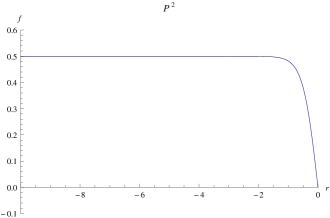
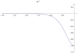
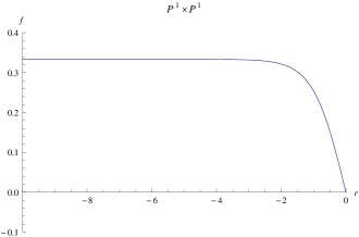
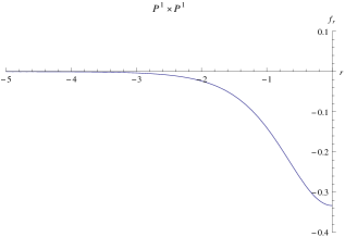
Of course, the above graphs of $f=f(r)$ just recover the graph $f(r)=-\frac{1}{2}\tanh(2r)$ for $\mathbb{P}^{2}$ and $f(r)=-\frac{1}{3}\tanh(r)$ for $\mathbb{P}^{1}\times\mathbb{P}^{1}$ (up to high precision).

If we choose different $\tau$, then we get different solution $f$, $h=f_{r}$. We know that $\lim_{r\rightarrow-\infty}f(r)=f(-\infty)=\alpha^{2}=\frac{1+2\beta}{6}$. Numerically, we can just evaluate $f(r)$ for $r$ being sufficiently negative to calculate $\alpha^{2}$. Actually, after several tests, one can observe that for fixed $\tau$, the graph will becomes flat as $r$ goes toward $-\infty$ which means $f(r)$ becomes stabilized. The speed of approaching flatness depends on the boundary value $h(0)=-\frac{1}{\tau}$. The bigger $\tau$ is, the longer $r$-distance it takes for the graph to become flat. (This is related to the bubbling phenomenon below)

We can use Mathematica to calculate (very dense) sequences of data for $\{\tau,f(\tau,r)\}$ where we make solution $f$ depend the boundary data $\tau$. Then we sample the value of $f(\tau,r)$ at $r=-500$. (One can certainly choose $r$ to be more negative but the visual effect does not change) Figure 3 shows the numerical result. The two subfigures are for short range and long range of $\tau$ respectively.

(a) short range

(b) long range

Figure 3: $(\tau,\alpha^{2})$

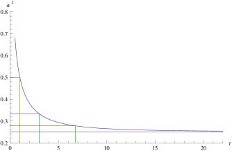
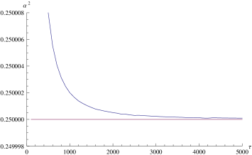
We see immediately that $\alpha^{2}$ is a decreasing function of $\tau$. More importantly, from the picture, we sees that one always has

$$\alpha^{2}=\frac{1+2\beta}{6}>0.25\Longleftrightarrow\beta>\frac{1}{4}.$$

and all the $\beta>\frac{1}{4}$ can be achieved. In particular, when $\beta=\frac{1}{3}$, where $\alpha^{2}=\frac{5}{18}=0.277777_{\dots}$, one can find approximate value of $\tau\sim 6.73$ from numerical result. In the picture, we have identified three special points: $(1,0.5)$,$(3,1/3)$ and $(6.73,\frac{5}{18})$ which corresponds to $\beta=1$, $\frac{1}{2}$ and $\frac{1}{3}$ respectively. The corresponding graph of $f$ and $h=f_{r}$ for $\tau=6.73(\beta=\frac{1}{3})$ is shown in figure 4.

(a) $(r,f)$

(b) $(r,f_{r})$

Figure 4: Data for $({\mathbb{P}}^{2},\frac{2}{3}D)$

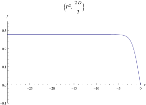
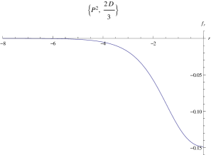
Finally, note that we are only interested when $\beta\leq 1$, or equivalently when $\alpha^{2}\leq 0.5$. However the picture suggests we can even pass $\beta\leq 1$ and solve for conic Kähler-Einstein metric with cone angle $2\pi\beta>2\pi$ along the conic curve.

5 Limit as $\beta$ goes to $1/4$

5.1 Metric Limit

We know that $SU(2)$ acts on $\mathbb{P}^{1}$ naturally. As pointed out in [4], the following embedding is equivariant with respect to the covering homomorphism $\phi:SU(2)\rightarrow SO(3,\mathbb{R})$.

$$\Delta:\mathbb{P}^{1} \longrightarrow \mathbb{P}^{2}$$

$${[U_{0},U_{1}]} \mapsto [U_{0}^{2}+U_{1}^{2},2iU_{0}U_{1},i(U_{0}^{2}-U_{1}^{2})].$$

Here $SU(2)$ acts on $\mathbb{P}^{2}(1,1,4)$ by acting on the first two variables:

$$g\cdot[U_{0},U_{1},V]=[g\cdot(U_{0},U_{1}),V].$$

Note that

$$\Delta(\mathbb{P}^{1})=\{Z_{1}^{2}+Z_{2}^{2}+Z_{3}^{2}=0\}.$$

Fix generators of $SU(2,\mathbb{C})$ to be standard Pauli matrices:

$$Y_{1}=\left(\begin{array}[]{cc}0&1\\ -1&0\end{array}\right),\;Y_{2}=\left(\begin{array}[]{cc}0&i\\ i&0\end{array}\right),\;Y_{3}=\left(\begin{array}[]{cc}i&0\\ 0&-i\end{array}\right).$$

Note that the commutator relation $[Y_{1},Y_{2}]=2Y_{3}$ and cyclicly. So by letting $\tilde{Y}_{i}=\frac{Y_{i}}{2}$, $\tilde{Y}_{i}$’s satisfy $[\tilde{Y}_{1},\tilde{Y}_{2}]=\tilde{Y}_{3}$ and cyclicly. For simplicity, we will still use $\tilde{Y}_{i}$ to denote the vector fields on $\mathbb{P}(1,1,4)$ corresponding to the infinitesimal actions of $\tilde{Y}_{i}$. Then we have

Lemma 5.1.

When we restrict to $\mathbb{P}^{1}$, $\Delta_{*}\tilde{Y}_{1}=-T_{u}$, $\Delta_{*}\tilde{Y}_{2}=T_{v}$, $\Delta_{*}\tilde{Y}_{3}=T_{w}$.

Proof.

$\Delta(1,0)=(1,0,i)=u+iv$ with $u=(1,0,0)$ and $v=(0,0,1)$. So $w=u\times v=-(0,1,0)$.

$$\Delta_{*}\tilde{Y}_{i}=(2(U_{0}\dot{U}_{0}+U_{1}\dot{U}_{1}),2i(\dot{U}_{0}U_{1}+U_{0}\dot{U}_{1}),2i(U_{0}\dot{U}_{0}-U_{1}\dot{U}_{1}))$$

1. $\tilde{Y}_{1}=\frac{1}{2}(U_{1},-U_{0})$, so

   $$\Delta_{*}\tilde{Y}_{1}=(0,-i(U_{0}^{2}-U_{1}^{2}),2iU_{0}U_{1}).$$

   In particular, $\tilde{Y}_{1}|_{(1,0)}=\frac{1}{2}(0,-1)$ and $\Delta_{*}\tilde{Y}_{1}|_{(1,0)}=(0,-i,0)=ie_{w}$. So $\Delta_{*}\tilde{Y}_{1}=-T_{u}$.

2. $\tilde{Y}_{2}=\frac{1}{2}(iU_{1},iU_{0})$, so

   $$\Delta_{*}\tilde{Y}_{2}=(2iU_{0}U_{1},-(U_{0}^{2}+U_{1}^{2}),0).$$

   In particular, $\tilde{Y}_{2}|_{(1,0)}=\frac{1}{2}(i,0)$, $\Delta_{*}\tilde{Y}_{2}|_{(1,0,i)}=(0,-1,0)=e_{w}$. So $\Delta_{*}\tilde{Y}_{2}=T_{v}$.

3. $\tilde{Y}_{3}=\frac{1}{2}(iU_{0},-iU_{1})$, so

   $$\Delta_{*}\tilde{Y}_{1}=(i(U_{0}^{2}-U_{1}^{2}),0,-(U_{0}^{2}+U_{1}^{2})).$$

   In particular, $\tilde{Y}_{3}|_{(1,0)}=\frac{i}{2}(1,0)$ and $\Delta_{*}\tilde{Y}_{3}|_{(1,0,i)}=(i,0,-1)=-v+iu$. So $\Delta_{*}\tilde{Y}_{3}=T_{w}$.

∎

We can define a function which classifies the $SU(2)$-orbits

$$\tilde{R}:\mathbb{P}(1,1,4) \longrightarrow [0,+\infty)$$

$${[U_{0},U_{1},V]} \mapsto \left(\frac{|U_{0}|^{2}+|U_{1}|^{2}}{|V|^{1/2}}\right)^{1/2}$$

Lemma 5.2.

The generic orbit when $0<\tilde{R}<\infty$ is isomorphic to $SU(2)/\mathbb{Z}_{4}\cong SO(3)/\mathbb{Z}_{2}$. The special orbit are

$${\rm Orb}_{\tilde{R}=0}={\rm Pt}=[0,0,1],\quad{\rm Orb}_{\tilde{R}=\infty}=\mathbb{P}^{1}.$$

Proof.

If $0<\tilde{R}<+\infty$, then $[U_{0},U_{1},V]$ is the same as $[\sqrt{-1}^{j}U_{0},\sqrt{-1}^{j}U_{1},V]$, $j=1,2,3,4$. So the stabilizer is isomorphic to $\mathbb{Z}_{4}$. The cases of special orbits are clear. ∎

Now the $SU(2)$-invariant Kähler metric has the form

$$g=dt^{2}+a^{2}\sigma_{1}^{2}+b^{2}\sigma_{2}^{2}+c^{2}\sigma_{3}^{2}.$$

Similar as the example 3.1 in Section 2, we can calculate the induced orbifold Kähler-Einstein metric by the branch covering map:

$$\mathbb{P}(1,1,1) \longrightarrow \mathbb{P}(1,1,4)$$

$${[Z_{1},Z_{2},Z_{3}]} \mapsto [Z_{1},Z_{2},Z_{3}^{4}].$$

Because the metric is $SU(2)$ invariant, to write down the metric we only need to calculate the length of the basic vector fields at the the special point $(\tilde{R},0,1)$ in each $SU(2)$-orbit.

1. $T_{\tilde{R}}|_{(\tilde{R},0,1)}=(1,0,0)$, $|T_{\tilde{R}}|=\frac{1}{1+\tilde{R}^{2}}.$

2. $\tilde{Y}_{1}|_{(\tilde{R},0,1)}=\frac{1}{2}(0,-\tilde{R},0)$, $a=|\tilde{Y}_{1}|_{g}=\frac{1}{2}\frac{\tilde{R}}{\sqrt{1+\tilde{R}^{2}}}$.

3. $\tilde{Y}_{2}|_{(\tilde{R},0,1)}=\frac{1}{2}(0,i\tilde{R},0)$, $b=|\tilde{Y}_{2}|_{g}=\frac{1}{2}\frac{\tilde{R}}{\sqrt{1+\tilde{R}^{2}}}$.

4. $\tilde{Y}_{3}|_{(\tilde{R},0,1)}=\frac{1}{2}(i\tilde{R},0,0)$, $c=|\tilde{Y}_{3}|_{g}=\frac{1}{2}\frac{\tilde{R}}{1+\tilde{R}^{2}}$.

Again, we can transform to the distance function:

$$dt=-\frac{d\tilde{R}}{1+\tilde{R}^{2}}\;\&\;\tilde{R}(+\infty)=0\Longrightarrow\tilde{R}=\tan(\pi/2-t),0\leq t\leq\pi/2.$$

By substituting $\tilde{R}$ into the expression of $a$, $b$ and $c$, we get the data for $\mathbb{P}(1,1,4)$:

$$a=b=\frac{1}{2}\sin\left(\frac{\pi}{2}-t\right)=\frac{1}{2}\cos(t).$$

$$c=\frac{1}{4}\sin(\pi-2t)=\frac{1}{4}\sin(2t).$$

Note that in this case, $a/b\equiv 1$. This is very different from the case where $\beta>1/4$. For the latter, $a<b$ except on the special fibre ${\rm Orb}_{R=1}\cong\mathbb{P}^{1}$ where $a=b$. Moreover, the boundary condition now becomes

$$a(t)=b(t) = 1/2+O(t^{2})$$

$$c(t) = \frac{1}{2}t+O(t^{3})$$

On the other end where $t_{*}=\pi/2$, $a(\pi/2)=b(\pi/2)=c(\pi/2)=0$. Geometrically, the special fibre ${\rm Orb}_{R=0}\cong\mathbb{RP}^{2}$ shrinks to a point as $\beta\rightarrow 1/4$. If we do the same transformation that $dr/dt=1/c$, the range of $r$ will becomes $(-\infty,+\infty)$ instead of $(-\infty,0)$ because $c(t_{*})=0$.

Next we give the numerical results which show that the metric $\omega_{\beta}$ converges to the orbifold Kähler-Einstein metric on $\mathbb{P}(1,1,4)$.

First we integrate the identity $dr/dt=1/c$ numerically and plot the relation between the boundary value $b(t_{*})^{2}=1/\tau$ and $t_{\max}=t_{*}$. We see that the maximal value for $t$ is an increasing function of $\tau$. As $\tau\rightarrow+\infty$, or equivalently as $\beta\rightarrow 1/4$, $t_{max}=t_{*}$ converges to $\pi/2$.

(a) short range

(b) long range

Figure 5: $(\tau,t_{max}=t_{*})$

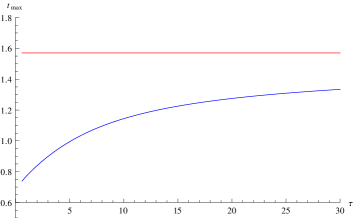
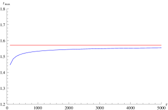
Note that the coordinate $t$ is the distance function from the special orbit $\mathbb{P}^{1}$. So $t$ is a geometrically meaningful coordinate in contrast with $r$ which is only an auxiliary coordinate. So we can get a good convergence when we look the data as functions $t$.

Now we can plot the graph of the data set $(f=ab,R=a/b,-f_{r}=c^{2})$ as the function of $t$ instead of $r$. (See (11)). Figure 6 shows the data for four $\tau$’s: $\tau=10^{i}$ for $i=1,2,3,4$. The corresponding colors and markers are “Blue Round”, “Green Square”, “Orange Diamond”, “Pink Triangle” for $i=1,2,3,4$ respectively. The “Red Upside-down Triangle” represent the data for $\mathbb{P}(1,1,4)$ where

$$f(t)=a(t)b(t)=\frac{1}{4}\cos^{2}(t),\quad R=\frac{a}{b}\equiv 1,\quad c^{2}(t)=\frac{1}{4}\sin^{2}(2t).$$

(a) $(t,f=ab)$

(b) $(t,a/b)$

(c) $(t,c^{2})$

Figure 6: Convergence of data

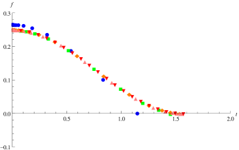
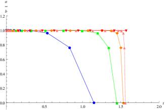
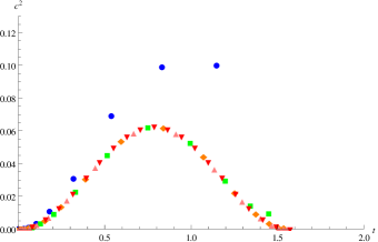
One can see that the data for $\tau$ large fits with the data for $\mathbb{P}(1,1,4)$ very well. Again, we know that $\tau$ going to $+\infty$ is equivalent to $\beta$ going to $1/4$. So the numerical result implies the expected result: as $\beta\rightarrow 1/4$, the metric $\omega_{\beta}$ converges to the orbifold Kähler-Einstein metric $\hat{\omega}_{KE}$ on $P(1,1,4)$.

5.2 $\mathbb{Z}_{2}$-quotient of Eguchi-Hanson as the Bubble

As pointed out by Dr. H-J. Hein and Professor Lebrun, if we rescale the metric near the orbit ${\rm Orb}_{R=0}=\mathbb{RP}^{2}$ appropriately, then the rescaled metrics should converge to another well known metric which is the $\mathbb{Z}_{2}$ quotient of the Eguchi-Hanson metric. This kind of metrics was studied in much generality by Stenzel [5]. It’s easy to see this convergence from the discussion in Section 3 and the following numerical results. For this we use the explicit description of this metric in [5, Section 7], which says that, away from the $\mathbb{RP}^{2}$ the $\mathbb{Z}_{2}$-quotient of Eguchi-Hanson metric can be pulled back to an $SO(3)$ invariant metric on $(0,\infty)\times SO(3)$ with the following expression:

$$g=\cosh s(ds)^{2}+\sinh s\tanh s(X_{1}^{*})^{2}+\cosh s((X_{2}^{*})^{2}+(X_{3}^{*})^{2}).$$ (12)

As before, we can let $a^{*}(s)=\sqrt{\sinh s\tanh s}$, $b^{*}(s)=c^{*}(s)=\sqrt{\cosh s}$. Let $t^{*}$ be the distance function to the orbit $\mathbb{RP}^{2}$. Then from (12), we see the following relation:

$$\frac{ds}{dt^{*}}=\frac{1}{\sqrt{\cosh s}}=\frac{1}{c^{*}(s)},\quad\frac{a^{*}}{b^{*}}(s)=\tanh s.$$

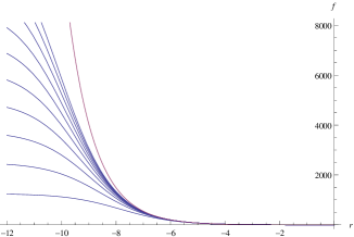
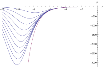
If we compare these identities with (8) and (9), we see that the coordinate $r$ is preserved under this convergence. In other words, $r=-s$ and $\frac{a^{*}}{b^{*}}=\frac{a}{b}=-\tanh r$. To prove the convergence, we only need to prove the convergence of rescaled data as functions of $r$. Note that, since the length scale of ${\rm Orb}_{R=0}=\mathbb{RP}^{2}$ is $1/\sqrt{\tau}$ as $\tau\rightarrow+\infty$ (equivalently as $\beta\rightarrow 1/4$), we need to use the scale factor $\tau$ to rescale the metric back. So we need to show the following convergence.

$$\lim_{\tau\rightarrow+\infty}f\tau=\lim_{\tau\rightarrow+\infty}a(r,\tau)b(r,\tau)\cdot\tau=a^{*}b^{*}=-\sinh r,$$

$$\lim_{\tau\rightarrow+\infty}f_{r}\tau=\lim_{\tau\rightarrow+\infty}-c(r,\tau)^{2}\tau=-(c^{*})^{2}=-\cosh r.$$

Figure 7 shows the convergence of numerical data for $\tau=5000*i$, $i=1,\cdots,10$.

(a) $(r,f)$

(b) $(r,f_{r})$

Figure 7: Bubbling

6 Data of ${\mathbb{P}}^{1}\times{\mathbb{P}}^{1}$ and associated Sasaki-Einstein metric

We have the following Segre embedding of ${\mathbb{P}}^{1}\times{\mathbb{P}}^{1}$ into ${\mathbb{P}}^{3}$ by the complete linear system $|H_{1}+H_{2}|$ where $H_{1}$ and $H_{2}$ are the hyperplane divisors of the two factors of ${\mathbb{P}}^{1}$ respectively.

$$\phi:\mathbb{P}^{1}\times\mathbb{P}^{1} \longrightarrow {\mathbb{P}}^{3}$$ (13)

$$([U_{0},U_{1}],[V_{0},V_{1}]) \mapsto [U_{0}V_{0}+U_{1}V_{1},{\sqrt{-1}}(U_{0}V_{0}-U_{1}V_{1}),U_{0}V_{1}+U_{1}V_{0},U_{0}V_{1}-U_{1}V_{0}].$$

Note that

$$\phi({\mathbb{P}}^{1}\times{\mathbb{P}}^{1})=\{[Z_{1},Z_{2},Z_{3},Z_{4}]\in{\mathbb{P}}^{3};Z_{1}^{2}+Z_{2}^{2}+Z_{3}^{2}=Z_{4}^{2}\}.$$

Lemma 6.1.

Let $p_{i}:{\mathbb{P}}^{1}\times{\mathbb{P}}^{1}\rightarrow{\mathbb{P}}^{1}$ be the projection to the $i-th$ ${\mathbb{P}}^{1}$-factor and $\omega_{{\mathbb{P}}^{N}}$ denote the standard Fubini-Study metric on ${\mathbb{P}}^{N}$ in the cohomology class $2\pi c_{1}(\mathcal{O}_{{\mathbb{P}}^{N}}(1))$, then the Segre embedding $\phi$ satisfies

$$\phi^{*}\omega_{{\mathbb{P}}^{2}}=p_{1}^{*}\omega_{{\mathbb{P}}^{1}}+p_{2}^{*}\omega_{\mathbb{P}^{1}}=:\tilde{\omega}.$$

Proof.

This follows from the following formula:

$$p_{1}^{*}\omega_{{\mathbb{P}}^{1}}+p_{2}^{*}\omega_{{\mathbb{P}}^{1}}={\sqrt{-1}\partial\bar{\partial}}\log((|U_{0}|^{2}+|U_{1}|^{2})(|V_{0}|^{2}+|V_{1}|^{2}))$$

$$= {\sqrt{-1}\partial\bar{\partial}}\log\left(|U_{0}V_{0}+U_{1}V_{1}|^{2}+|{\sqrt{-1}}(U_{0}V_{0}-U_{1}V_{1})|^{2}+|U_{0}V_{1}+U_{1}V_{0}|^{2}+|U_{0}V_{1}-U_{1}V_{0}|^{2}\right).$$

∎

Now $SO(3)$ acts on $\mathbb{C}^{4}$ by

$$g\cdot(Z_{1},Z_{2},Z_{3},Z_{4})=(g\cdot(Z_{1},Z_{2},Z_{3}),Z_{4}).$$

This induces an action of $SO(3)$ on $\phi({\mathbb{P}}^{1}\times{\mathbb{P}}^{1})$.

We will calculate the data associated with the product metric $\tilde{\omega}:=p_{1}^{*}\omega_{{\mathbb{P}}^{1}}+p_{2}^{*}\omega_{{\mathbb{P}}^{1}}$. Use the similar method as in Section 2 we use the following notation:

$$(Z_{1},Z_{2},Z_{3},Z_{4})\sim e^{-i{\rm Arg}(Z_{1}^{2}+Z_{2}^{2}+Z_{3}^{2})/2}(Z_{1},Z_{2},Z_{3},Z_{4})=:(u+iv,z_{4}).$$

Here $u,v\in\mathbb{R}^{3}$, $z_{4}\in\mathbb{C}$. In this notation, we have

$$\phi({\mathbb{P}}^{1}\times{\mathbb{P}}^{1})=\{(u+iv,z_{4});|u|^{2}-|v|^{2}=z_{4}^{2},0\neq(u+iv,z_{4})\in\mathbb{C}^{3}\times\mathbb{R}\}/\mathbb{R}^{\times}.$$

We can calculate the infinitesimal vector field of basis of $so(3)$, at point $(u+iv,\sqrt{|u|^{2}-|v|^{2}})$:

$$T_{u}=(-\sqrt{-1}|v|e_{w},0),\quad T_{v}=(|u|e_{w},0),\quad T_{w}=(-|u|e_{v}+\sqrt{-1}|v|e_{u},0).$$

As in Section 3.1, we define $R=\frac{|v|}{|u|}$ and calculate the radial vector field as

$$\quad T_{R}=\left({\sqrt{-1}}|u|e_{v},-\frac{|u|R}{\sqrt{1-R^{2}}}\right).$$

Here for clarify, we will use $\overline{T}_{u}$, $\overline{T}_{v}$, $\overline{T}_{w}$ and $\overline{T}_{R}$ to denote the tangent vector in $T_{[u+iv]}\mathbb{P}^{2}$ determined by $T_{u},T_{v},T_{w},T_{R}$ respectively. The lengths of these tangent vectors in $T_{[u+iv,iz_{3}]}\phi({\mathbb{P}}^{1}\times{\mathbb{P}}^{1})$ can be calculated as in Example 3.1:

$$|\overline{T}_{u}|_{\tilde{\omega}}^{2}=\frac{R^{2}}{2},\quad|\overline{T}_{v}|_{\tilde{\omega}}^{2}=\frac{1}{2},\quad|\overline{T}_{w}|_{\tilde{\omega}}^{2}=\frac{1-R^{2}}{2},\quad|\overline{T}_{R}|_{\tilde{\omega}}^{2}=\frac{1}{2(1-R^{2})}.$$

By transforming the variable $R$ into the distance variable $\tilde{t}$ under the metric $\tilde{\omega}$, we get:

$$\frac{d\tilde{t}}{dR}=\frac{1}{2(1-R^{2})}\;\&\;\tilde{t}(1)=0\Longrightarrow R(\tilde{t})=\cos(\sqrt{2}\tilde{t}),0\leq\tilde{t}\leq\frac{\pi}{2\sqrt{2}}.$$ (14)

$$|\overline{T}_{u}|_{\tilde{\omega}}=\frac{1}{\sqrt{2}}\cos(\sqrt{2}\tilde{t}),\quad|\overline{T}_{v}|_{\tilde{\omega}}=\frac{1}{\sqrt{2}},\quad|\overline{T}_{w}|_{\tilde{\omega}}=\frac{1}{\sqrt{2}}\sin(\sqrt{2}\tilde{t}).$$

Note that $\tilde{\omega}=p_{1}^{*}\omega_{{\mathbb{P}}^{1}}+p_{2}^{*}\omega_{{\mathbb{P}}^{1}}$ has Ricci curvature equal to 4. To normalize Ricci curvature to be 6, we just need to rescale the metric. So by letting $\omega=\frac{2}{3}\omega_{{\mathbb{P}}^{1}\times{\mathbb{P}}^{1}}$ and redefining $t=\sqrt{2}\tilde{t}/\sqrt{3}$ we get the following result, which are the same data as in Example 3.2

$$a=\frac{1}{\sqrt{3}}\cos(\sqrt{3}t),\quad b=\frac{1}{\sqrt{3}},\quad c=\frac{1}{\sqrt{3}}\sin(\sqrt{3}t);\quad 0\leq t\leq\frac{\pi}{2\sqrt{3}}.$$ (15)

Let ${\rm Aff}({\mathbb{P}}^{1}\times{\mathbb{P}}^{1})$ be the affine cone over $\phi({\mathbb{P}}^{1}\times{\mathbb{P}}^{1})\subset{\mathbb{P}}^{3}$:

$${\rm Aff}({\mathbb{P}}^{1}\times{\mathbb{P}}^{1})=\{(Z_{1},Z_{2},Z_{3},Z_{4})\in\mathbb{C}^{4};Z_{1}^{2}+Z_{2}^{2}+Z_{3}^{2}=Z_{4}^{2}\}.$$

In the following, we use $L$ to denote the total space of the line bundle $p_{1}^{*}\mathcal{O}(-H_{1})+p_{2}^{*}\mathcal{O}(-H_{2})$. Then $L=Bl_{0}{\rm Aff}({\mathbb{P}}^{1}\times{\mathbb{P}}^{1})$. In other words, the zero section $S_{0}$ of $L$ can be blow-down to get a singular variety $L/S_{0}$ which is isomorphic to the affine cone ${\rm Aff}({\mathbb{P}}^{1}\times{\mathbb{P}}^{1})$. Moreover, line bundle $L$ has a Hermitian metric $h:=h_{{\mathbb{P}}^{1}\times{\mathbb{P}}^{1}}$ whose curvature is $-\tilde{\omega}=-(p_{1}^{*}\omega_{{\mathbb{P}}^{1}}+p_{2}^{*}\omega_{{\mathbb{P}}^{1}})$, i.e. we have the identity:

$$-{\sqrt{-1}\partial\bar{\partial}}\log h=-\tilde{\omega}=-(p_{1}^{*}\omega_{{\mathbb{P}}^{1}}+p_{2}^{*}\omega_{{\mathbb{P}}^{1}}).$$ (16)

Now $h:L\ni s\rightarrow|s|_{h}^{2}$ is a smooth function on $L$ which induces a smooth function $h$ on $L/S_{0}\cong{\rm Aff}({\mathbb{P}}^{1}\times{\mathbb{P}}^{1})$. Up to a scaling factor, we see that

$$h:{\rm Aff}({\mathbb{P}}^{1}\times{\mathbb{P}}^{1}) \rightarrow \mathbb{R}^{\geq 0}$$

$$(Z_{1},Z_{2},Z_{3},Z_{4}) \mapsto |Z|^{2}=|Z_{1}|^{2}+|Z_{2}|^{2}+|Z_{3}|^{2}+|Z_{4}|^{2}.$$

Define $M^{5}\subset L$ to be the unit circle bundle, i.e. $M^{5}=\{s\in L;|s|_{h}^{2}=1\}$. Then

$$M^{5}\cong\{(Z_{1},Z_{2},Z_{3},Z_{4});Z_{1}^{2}+Z_{2}^{2}+Z_{3}^{2}=Z_{4}^{2},|Z|^{2}=1\}={\rm Aff}({\mathbb{P}}^{1}\times{\mathbb{P}}^{1})\cap S^{7}.$$

We know that there exists a Sasaki-Einstein metric on $M^{5}$. Now we will calculate this Sasaki-Einstein metric on $M^{5}$ by calculating the data in the sense of [1]. To do this we will first calculate the metric on $M^{5}$ induced by the standard Euclidean metric on $\mathbb{C}^{4}$. Then we modify the metric appropriately (rescale it in different directions) to get the desired Sasaki-Einstein metric.

Lemma 6.2.

On $M^{5}=S^{7}\cap{\rm Aff}({\mathbb{P}}^{1}\times{\mathbb{P}}^{1})$, we have

$$|u|=\frac{1}{\sqrt{2}},\quad|v|=\frac{\cos(\sqrt{2}\tilde{t})}{\sqrt{2}}.$$ (17)

Proof.

On $M^{5}$, we have the identities $|u|^{2}-|v|^{2}=z_{4}^{2}$ and $|u|^{2}+|v|^{2}+|z_{4}|^{2}=1$. So we get $|u|=1/\sqrt{2}$. The second identity follows from (14) and $|v|=R|u|$. ∎

Now $G=SO(3)\times U(1)$ acts on $\mathbb{C}^{4}$ by

$$(g,e^{i\theta})\cdot(Z_{1},Z_{2},Z_{3},Z_{4})=\left(e^{i\theta}g(Z_{1},Z_{2},Z_{3}),e^{i\theta}Z_{4}\right).$$

The generic orbit is of codimension 1. ${\rm Aff}({\mathbb{P}}^{1}\times{\mathbb{P}}^{1})$ is $G$-invariant under this action. Fix the standard basis of $so(3)\oplus u(1)$ by adjoining the generator $X_{4}$ of $u(1)$ to the standard basis of $so(3)$ used above. We will denote the infinitesimal vector fields by the same notation. So we have

$$X_{1}=T_{u},X_{2}=T_{v},X_{3}=T_{w},X_{4}=(-v+iu,iz_{4}).$$

Proposition 6.1.

Considering $M^{5}$ as a submanifold in $(\mathbb{C}^{4},g_{{\rm flat}})$, $T_{(u+iv,z_{4})}\mathbb{C}^{4}=\mathbb{R}^{8}$ has an orthonormal basis given by

$$\partial_{\tilde{r}} = (u+iv,z_{4})$$

$${\tilde{\mathfrak{e}}}_{0} = \partial_{\theta}=X_{4}=(-v+iu,iz_{4}),$$

$$\tilde{\mathfrak{e}}_{1} = \partial_{\tilde{t}}=-\sqrt{2}\sin(\sqrt{2}\tilde{t})T_{R}=(-{\sqrt{-1}}\sin(\sqrt{2}\tilde{t})e_{v},\cos(\sqrt{2}\tilde{t})),$$

$$\tilde{\mathfrak{e}}_{2} = \frac{\sqrt{2}}{\sin(\sqrt{2}\tilde{t})}(-X_{3}+\cos(\sqrt{2}\tilde{t})X_{4})=(\sin(\sqrt{2}\tilde{t})e_{v},{\sqrt{-1}}\cos(\sqrt{2}\tilde{t})),$$

$$\tilde{\mathfrak{e}}_{3} = \frac{\sqrt{2}}{\cos(\sqrt{2}\tilde{t})}X_{1}=(-{\sqrt{-1}}e_{w},0),$$

$$\tilde{\mathfrak{e}}_{4} = \sqrt{2}X_{2}=(e_{w},0).$$

We have the relation

$$J\partial_{\tilde{r}}=i\partial_{\tilde{r}}=\partial_{\theta},\quad J{\tilde{\mathfrak{e}}}_{1}=i{\tilde{\mathfrak{e}}}_{1}={\tilde{\mathfrak{e}}}_{2},\quad J{\tilde{\mathfrak{e}}}_{3}=i{\tilde{\mathfrak{e}}}_{3}={\tilde{\mathfrak{e}}}_{4}.$$

Under the induced metric on $M^{5}$ by the standard Euclidean metric on $\mathbb{C}^{4}$, $T_{(u+iv,z_{4})}M^{5}$ has an orthonormal basis $\{\partial_{\theta},{\tilde{\mathfrak{e}}}_{1},{\tilde{\mathfrak{e}}}_{2},{\tilde{\mathfrak{e}}}_{3},{\tilde{\mathfrak{e}}}_{4}\}$. Moreover, let $S^{1}\rightarrow M^{5}\rightarrow{\mathbb{P}}^{1}\times{\mathbb{P}}^{1}$ be the fibration structure. Then the vertical unit vector field is generated by $\partial_{\theta}$, and the space of horizontal vector fields in the tangent space has an orthonormal basis consisting of $\{{\tilde{\mathfrak{e}}}_{1},{\tilde{\mathfrak{e}}}_{2},{\tilde{\mathfrak{e}}}_{3},{\tilde{\mathfrak{e}}}_{4}\}$.

Proof.

First it’s easy to see that $J\partial_{\tilde{r}}=\partial_{\theta}$ and $\partial_{\tilde{r}}\perp Span(\{\partial_{\theta},X_{i},i=1,2,3,4\})$. We can also verify that $Span\{X_{1},X_{2}\}\perp Span(\{\partial_{\theta},X_{3},X_{4}\})$ and $T_{R}\perp Span(\{\partial_{\theta},X_{i},i=1,2,3,4\})$. The Lemma follows by orthonormalization. ∎

Lemma 6.3.

Considering $h$ as a smooth function on $L$ as above, Sasaki-Einstein metric on $M^{5}$ is given by

$$g_{SE}=\frac{1}{2}\left.({\sqrt{-1}\partial\bar{\partial}}h^{2/3})(\cdot,J\cdot)\right|_{M^{5}}.$$

Proof.

If $M^{5}$ is a Sasaki-Einstein metric, then the metric cone $C(M^{5})$ is a Ricci-flat Kähler metric. In our case, $C(M^{5})\cong L/S_{0}$ as the affine variety with an isolated singular point. So we only need to construct the rotationally symmetric Ricci-flat Kähler metric on $C(M^{5})\cong L/S_{0}$ and restrict to $M^{5}\cong\{h=1\}\cap C(M^{5})$ to get the Sasaki-Einstein metric on $M^{5}$.

In general, assume $L\rightarrow D_{0}$ be a line bundle with a Hermitian metric $h$ such that ${\sqrt{-1}\partial\bar{\partial}}\log h=\tilde{\omega}$ is a Kähler-Einstein metric, satisfying $Ric(\tilde{\omega})=\tau\tilde{\omega}$. Then we can define the rotationally symmetric Kähler metric on the total space on $L/S_{0}$ using the potential $h^{\delta}$, i.e. we define

$$\Omega_{\delta}={\sqrt{-1}\partial\bar{\partial}}h^{\delta}=\delta h^{\delta}\tilde{\omega}+\delta^{2}h^{\delta}\frac{\nabla\xi\wedge\overline{\nabla\xi}}{|\xi|^{2}}.$$ (18)

The Ricci curvature of $\Omega_{\delta}$ on $L\backslash D_{0}$ is equal to

$$Ric(\Omega_{\delta}) = -{\sqrt{-1}\partial\bar{\partial}}\log\Omega_{\delta}^{n}=-(d+1){\sqrt{-1}\partial\bar{\partial}}\log h^{\delta}+Ric(\tilde{\omega})$$

$$= \pi^{*}(-(d+1)\delta\tilde{\omega}+\tau\tilde{\omega}).$$

This is zero if and only if $\delta=\tau/(d+1)$. In our case, $\tau=2$, $d=2$. So $\delta=2/3$. ∎

Theorem 6.1.

The Sasaki-Einstein metric on $M^{5}$ has an orthonormal basis given by

$$\mathfrak{e}_{0} = \frac{3}{2}X_{4},$$

$$\mathfrak{e}_{1} = \partial_{t}=-\sqrt{3}\sin(\sqrt{3}t)T_{R},$$

$$\mathfrak{e}_{2} = \frac{\sqrt{3}}{\sin(\sqrt{3}t)}(-X_{3}+\cos(\sqrt{3}t)X_{4}),$$

$$\mathfrak{e}_{3} = \frac{\sqrt{3}}{\cos(\sqrt{3}t)}X_{1},$$

$$\mathfrak{e}_{4} = \sqrt{3}X_{2}.$$

Proof.

First note that, the induced metric on $M^{5}$ by flat metric is given by $\frac{1}{2}{\sqrt{-1}\partial\bar{\partial}}h$. By the formula (18), we see that if we change the potential from $h$ to $h^{\delta}$, then the vertical metric scales by $\delta^{2}$, and the horizontal part of the metric scales by $\delta$. Since $\delta=2/3$ now, the Theorem follows from Proposition 6.1. ∎

Corollary 6.1.

1. Under the Sasaki-Einstein metric on $M^{5}$, there is an orthonormal basis of $T^{*}M^{5}$ given by

   $$\alpha:=\frac{2}{3}(X_{4}^{*}+\cos(\sqrt{3}t)X_{3}^{*}),$$

   $${\mathfrak{e}}^{1}=dt,\quad{\mathfrak{e}}^{2}=-\frac{\sin(\sqrt{3}t)}{\sqrt{3}}X_{3}^{*},$$

   $${\mathfrak{e}}^{3}=\frac{\cos(\sqrt{3}t)}{\sqrt{3}}X_{1}^{*},\quad{\mathfrak{e}}^{4}=\frac{1}{\sqrt{3}}X_{2}^{*}.$$

2. If we define $\omega_{1}=e^{1}\wedge e^{2}+e^{3}\wedge e^{4}$, $\omega_{2}=e^{1}\wedge e^{3}+e^{4}\wedge e^{2}$ and $\omega_{3}=e^{1}\wedge e^{4}+e^{2}\wedge e^{3}$, the following identities hold:

   $$d\alpha=2\omega_{1},\quad d\omega_{2}=-3\alpha\wedge\omega_{3}+2X_{4}^{*}\wedge\omega_{3},\quad d\omega_{3}=3\alpha\wedge\omega_{2}-2X_{4}^{*}\wedge\omega_{2}.$$

   This gives the $SU(2)$ structure in the sense of [1].

Remark 6.1.

The item 2 in Corollary 6.1 follows from Item 1 and the fomula $dX_{i}^{*}=-\epsilon_{ijk}X_{j}^{*}\wedge X_{k}^{*}$. As explained in [1], because we are using the $G$-invariant forms on $G\times(t_{-},t_{+})$ to represent the data, there is an extra term $2X_{4}^{*}\wedge\omega_{3}$. The coefficient $2$ comes from the fact that $(e^{i\theta})^{*}\mathcal{S}=e^{2i\theta}\cdot\mathcal{S}$ where we use $\mathcal{S}$ to denote the nonwhere vanishing holomorphic volume form on $\mathcal{M}={\rm Aff}({\mathbb{P}}^{1}\times{\mathbb{P}}^{1})$ which can be given by the Poincaré residue formula:

$$\mathcal{S}=Res_{\mathcal{M}}(dZ_{1}\wedge dZ_{2}\wedge dZ_{3}\wedge dZ_{4})=-\frac{dZ_{1}\wedge dZ_{2}\wedge dZ_{3}}{Z_{4}}.$$

Remark 6.2.

By the similar calculation, we can calculate the data associated on the standard round $S^{5}$ under the $SO(3)$ action:

$$g\cdot(Z_{1},Z_{2},Z_{3})=\left(g(Z_{1},Z_{2},Z_{3})\right).$$

The result is as follows. For the orthonormal basis of $TS^{5}$, we have

$${\mathfrak{e}}_{0}=\partial_{\theta}=X_{4},$$

$${\mathfrak{e}}_{1}=\partial_{t},\quad{\mathfrak{e}}_{2}=\frac{1}{\sin(2t)}(-X_{3}+\cos(2t)X_{4}),$$

$${\mathfrak{e}}_{3}=\frac{X_{1}}{\sin\left(\frac{\pi}{4}-t\right)},\quad{\mathfrak{e}}_{4}=\frac{X_{2}}{\cos\left(\frac{\pi}{4}-t\right)}.$$

So the corresponding orthonormal basis of $T^{*}S^{5}$ is

$$\alpha:={\mathfrak{e}}^{0}=X_{4}^{*}+\cos(2t)X_{3}^{*},$$

$${\mathfrak{e}}^{1}=dt,\quad{\mathfrak{e}}^{2}=-\sin(2t)X_{3}^{*},$$

$${\mathfrak{e}}^{3}=\sin\left(\frac{\pi}{4}-t\right)X_{1}^{*},\quad{\mathfrak{e}}^{4}=\cos\left(\frac{\pi}{4}-t\right)X_{2}^{*}.$$

The corresponding $SU(2)$-structural equations are:

$$d\alpha=2\omega_{1},\quad d\omega_{2}=-3\alpha\wedge\omega_{3}+3X_{4}^{*}\wedge\omega_{3},\quad d\omega_{3}=3\alpha\wedge\omega_{2}-3X_{4}^{*}\wedge\omega_{2}.$$

Remark 6.3.

There is a statement in Theorem 1 in [1]: “There is no solution of (23) that defines an Einstein-Sasaki metric on a compact manifold”. The above two special examples show that this statement is wrong. By going through the proof, we find that the error happens in Lemma 4, where, in the second case, the assumption $q\neq 0$ is made. In our notation, this implies the isotopy group of special orbit has a generator whose $X_{4}$-component is nonzero. But this is not true in the above examples. Actually, it’s easy to verify that

1. For $t=0$, $H_{-}\cong U(1)$ with Lie algebra $\mathfrak{h}=\langle-X_{3}+X_{4}\rangle$.

2. For $t=\frac{\pi}{2\sqrt{3}}$, $H_{+}\cong U(1)=U(1)_{1}$ with Lie algbra $\mathfrak{h}=\langle X_{1}\rangle$.

Because the action $U(1)_{1}$ has generator $X_{1}$ which has no contribution from $X_{4}$, so $q=0$ for $H_{+}$. It would be interesting to classify the missing cohomogeneity one Sasaki-Einstein 5-manifolds for which $q=0$.

7 Appendix

The following are the codes of Mathematica generating the figures appeared above.

1. Figure 1

   s = NDSolve[ {f’[t] == h[t], h’[t] == 12 f[t]*h[t] + 2 Coth[2 t]*h[t] - h[t]^2/f[t], f[-10^(-5)] == 10^(-5), h[-10^(-5)] == -1}, {f, h}, {t, -100, -10^(-5)}];

   Plot[Evaluate[h[t] /. s], {t, -3, -10^(-5)}, AxesLabel -$>$ {r, Subscript[f, r]}, PlotRange -$>$ {{-3, 0}, {-1.2, 0.2}}, PlotLabel -$>$ P^2]

   Plot[Evaluate[h[t] /. s], {t, -3, -10^(-5)}, AxesLabel -$>$ {r, Subscript[f, r]}, PlotRange -$>$ {{-3, 0}, {-1.2, 0.2}}, PlotLabel -$>$ P^2]

2. Figure 2

   s1 = NDSolve[{f’[t] == h[t], h’[t] == 12 f[t]*h[t] + 2 Coth[2 t]*h[t] - h[t]^2/f[t], f[-10^(-5)] == 10^(-5)/3, h[-10^(-5)] == -1/3}, {f, h}, {t, -100, -10^(-5)}];

   Plot[Evaluate[f[t] /. s1], {t, -10, -10^(-5)}, PlotRange -$>$ {{-10, -10^(-5)}, {-0.1, 0.4}}, PlotLabel -$>$ Superscript[P, 1]$\times$ Superscript[P, 1], AxesLabel -$>$ {r, f}]

   Plot[Evaluate[h[t] /. s1], {t, -5, -10^(-5)}, AxesLabel -$>$ {r, Subscript[f, r]}, PlotRange -$>$ {{-5, 0}, {-0.4, 0.1}}, PlotLabel -$>$ Superscript[P, 1]$\times$Superscript[P, 1]]

3. Figure 3

   1. Figure 3(a)

      Array[p,300]; For[i = 0, i $<$ 300, i++, {v = NDSolve[{f’[t] == h[t], h’[t] == 12 f[t]*h[t] + 2 Coth[2 t]*h[t] - h[t]^2/f[t], f[-10^(-5)] == 10^(-5)/(0.5 + 0.1*i), h[-10^(-5)] == -1/(0.5 + 0.1*i)}, {f, h}, {t, -500, -10^(-5)}], p[i + 1] = Evaluate[f[-500] /. v]}];

      ListLinePlot[{Table[{0.5 + 0.1*i, Extract[p[i + 1], 1]}, {i, 0, 300}], Table[{0 + 0.1*i, 0.25}, {i, 0, 300}], Table[{1, 0.05*i}, {i, 0, 10}], Table[{3, 1/3*0.1*i}, {i, 0, 10}], Table[{0.1*i, 0.5}, {i, 0, 10}], Table[{0.3*i, 1/3}, {i, 0, 10}], Table[{0.673*i, 5/18}, {i, 0, 10}], Table[{6.73, 5/180*i}, {i, 0, 10}]}, PlotRange -$>$ {{0, 22}, {0.2, 0.8}}, AxesLabel -$>$ {$\backslash$[Tau], $\backslash$[Alpha]^2}]

   2. Figure 3(b)

      Array[p, 50]; For[i = 1, i $<$ 51, i++, {v = NDSolve[{f’[t] == h[t], h’[t] == 12 f[t]*h[t] + 2 Coth[2 t]*h[t] - h[t]^2/f[t], f[-10^(-5)] == 10^(-5)/(100*i), h[-10^(-5)] == -1/(100*i)}, {f, h}, {t, -500, 10^(-4)}], p[i] = Evaluate[f[-500] /. v]}];

      ListLinePlot[{Table[{100*i, Extract[p[i], 1]}, {i, 1, 50}], Table[{100*i, 1/4}, {i, 1, 50}]}, PlotRange -$>$ {{0, 5000}, {0.249998, 0.250008}}, AxesLabel -$>$ {$\backslash$[Tau], $\backslash$[Alpha]^2}]

4. Figure 4

   v = NDSolve[{f’[t] == h[t], h’[t] == 12 f[t]*h[t] + 2 Coth[2 t]*h[t] - h[t]^2/f[t], f[-10^(-5)] == 10^(-5)/6.73, h[-10^(-5)] == -1/6.73}, {f, h}, {t, -100, -10^(-5)}];

   Plot[Evaluate[f[t] /. v], {t, -40, -10^(-5)}, AxesLabel -$>$ {r, f}, PlotRange -$>$ {{-30, -10^(-5)}, {-0.1, 0.35}}, PlotLabel -$>$ {P^2, 2/3 D}]

   Plot[Evaluate[h[t] /. v], {t, -8, -10^(-5)}, AxesLabel -$>$ {r, Subscript[f, r]}, PlotRange -$>$ {{-8, 0}, {-0.16, 0.01}}, PlotLabel -$>$ {P^2, 2/3 D}]

5. Figure 5

   1. Figure 5(a)

      Array[q, 200]; For[k = 1, k $<$ 201, k++, q[k] = 0]; For[i = 1, i $<$ 201, i++, {u = NDSolve[{f’[t] == h[t], h’[t] == 12 f[t]*h[t] + 2 Coth[2 t]*h[t] - h[t]^2/f[t], f[-10^(-5)] == 10^(-5)/(0.5 + 0.1*i), h[-10^(-5)] == -1/(0.5 + 0.1*i)}, {f, h}, {t, -300, -0.01}], For[j = 0, -300 + 0.01*j $<$ -0.01, j++, q[i] = q[i] + Sqrt[-Evaluate[h[-300 + 0.01*j] /. u]]*0.01]} ];

      ListLinePlot[{Table[{0.5 + 0.1*i, Re[Extract[q[i], 1]]}, {i, 1, 300}], Table[{0.5 + 0.1*i, Pi/2}, {i, 1, 300}]}, PlotRange -$>$ {{0, 30}, {0.5, 1.8}}, PlotStyle -$>$ {Blue, Red}, AxesLabel -$>$ {$\backslash$[Tau], Subscript[t, max]}]

   2. Figure 5(b)

      Array[p, 50]; Array[q, 50]; For[k = 1, k $<$ 51, k++, q[k] = 0]; For[i = 1, i $<$ 51, i++, {u = NDSolve[{f’[t] == h[t], h’[t] == 12 f[t]*h[t] + 2 Coth[2 t]*h[t] - h[t]^2/f[t], f[-10^(-5)] == 10^(-5)/(100*i), h[-10^(-5)] == -1/(100*i)}, {f, h}, {t, -300, -0.01}], p[i] = Evaluate[f[-300] /. u], For[j = 0, -300 + 0.005*j $<$ -0.01, j++, q[i] = q[i] + Sqrt[-Evaluate[h[-300 + 0.005*j] /. u]]*0.005]} ];

      ListLinePlot[{Table[{100*i, Re[Extract[q[i], 1]]}, {i, 1, 50}], Table[{100*i, Pi/2}, {i, 1, 50}]}, PlotRange -$>$ {{0, 5000}, {1.2, 1.8}}, PlotStyle -$>$ {Blue, Red}, AxesLabel -$>$ {$\backslash$[Tau], Subscript[t, max]}]

6. Figure 6

   n = 4; Array[p, {n, 300}] ; Array[q, {n, 300}]; Array[R, {n, 300}]; Array[c, {n, 300}]; For[i = 1, i $<$ 5, i++, {s = 0, u = NDSolve[{f’[t] == h[t], h’[t] == 12 f[t]*h[t] + 2 Coth[2 t]*h[t] - h[t]^2/f[t], f[-10^(-5)] == 10^(-5)/(10^i), h[-10^(-5)] == -1/(10^i)}, {f, h}, {t, -300, -0.0001}], For[k = 0, -300 + k $<$ -0.01, k++, {For[j = 0, j $<$ 1000, j++, {s = s + Sqrt[-Evaluate[h[-300 + k + 0.001*j] /. u]]*0.001}], p[i, k + 1] = Re[s], q[i, k + 1] = Evaluate[f[-300 + k + 0.001*j] /. u], R[i, k + 1] = -Tanh[-300 + k + 0.001*j], c[i, k + 1] = Evaluate[-h[-300 + k + 0.001*j] /. u]} ]}];

   ListPlot[ Join[Table[ Table[{Extract[p[i, n], 1], Extract[q[i, n], 1]}, {n, 1, 300}], {i, 1, 4}], {Table[{Pi*i/40, (1 + Cos[Pi*i/20])/8}, {i, 1, 20}]}], PlotRange -$>$ {{0, 2}, {-0.1, 0.3}}, PlotStyle -$>$ {Blue, Green, Orange, Pink, Red}, PlotMarkers -$>$ Automatic, AxesLabel -$>$ {t, f}]

   ListLinePlot[ Join[Table[ Table[{Extract[p[i, n], 1], R[i, n]}, {n, 1, 300}], {i, 1, 4}], {Table[{Pi*i/20, 1}, {i, 1, 10}]}], PlotRange -$>$ {{0, 2}, {-0.1, 1.2}}, PlotStyle -$>$ {Blue, Green, Orange, Pink, Red}, PlotMarkers -$>$ Automatic, AxesLabel -$>$ {t, a/b}]

   ListPlot[ Join[Table[ Table[{Extract[p[i, n], 1], Extract[c[i, n], 1]}, {n, 1, 300}], {i, 1, 4}], {Table[{Pi*i/40, (1 - Cos[i*Pi/10])/32}, {i, 1, 20}]}], PlotRange -$>$ {{0, 2}, {0, 0.13}}, PlotStyle -$>$ {Blue, Green, Orange, Pink, Red}, PlotMarkers -$>$ Automatic, AxesLabel -$>$ {t, c^2}]

7. Figure 7

   u = Table[{u = NDSolve[{f’[t] == h[t], h’[t] == 12 f[t]*h[t] + 2 Coth[2 t]*h[t] - h[t]^2/f[t], f[-10(̂-5)] == 10^(-5)/(5000*i), h[-10(̂-5)] == -1/(5000*i)}, {f, h}, {t, -300, -0.0001}]}, {i, 1, 10}];

   Plot[{Table[Evaluate[f[t] /. Extract[u, i]]*5000*i, {i, 1, 10}], Sinh[-t]}, {t, -12, 0}, AxesLabel -$>$ {r, f}]

   Plot[{Table[ Evaluate[h[t] /. Extract[u, i]]*5000*i, {i, 1, 10}], -Cosh[ t]}, {t, -12, -10^(-5)}, AxesLabel -$>$ {r, Subscript[f, r]}]

Chi Li
Department of Mathematics, SUNY at Stony Brook.
Email Address: chi.li@stonybrook.edu

References

- [1] Diego Conti: Cohomogeneity one Einstein-Sasaki 5-manifolds. Comm. Math. Phys. 274 (2007), no. 3, 751-774.
- [2] Andrew S. Dancer, and Ian A.B.Strachan: Kähler-Einstein metrics with action. Math. Proc. Camb. Phil. Soc. (1994), 115, 513.
- [3] J. Gauntlett, D. Martelli, J. Sparks, S-T. Yau: Obstructions to the existence of Sasaki-Einstein metrics. Comm. Math. Phys. 273 (2007), no. 3, 803-827.
- [4] Chi Li, and Song Sun: conical Kähler-Einstein metric revisited. arXiv:1207.5011.
- [5] Matthew B. Stenzel: Ricci-flat metrics on the complexification of a compact rank one symmetric space. Manuscripta Mathematica, Vol 80, No 1 (1993), 151-163.