The blockage problem

Abstract

We investigate the totally asymmetric exclusion process on ${\mathbb{Z}}$, with the jump rate at site $i$ given by $r_{i}=1$ for $i\neq 0$, $r_{0}=r$. It is easy to see that the maximal stationary current $j(r)$ is nondecreasing in $r$ and that $j(r)=1/4$ for $r\geq 1$; it is a long outstanding problem to determine whether or not the critical value $r_{c}$ of $r$ such that $j(r)=1/4$ for $r>r_{c}$ is strictly less than 1. Here we present a heuristic argument, based on the analysis of the first sixteen terms in a formal power series expansion of $j(r)$ obtained from finite volume systems, that $r_{c}=1$ and that for $r\lessapprox 1$, $j(r)\simeq{1/4}-\gamma\exp[-{a/(1-r)}]$ with $a\approx 2$. We also give some new exact results about this system; in particular we prove that $j(r)=J_{\rm max}(r)$, with $J_{\rm max}(r)$ the hydrodynamic maximal current defined by Seppäläinen, and thus establish continuity of $j(r)$. Finally we describe a related exactly solvable model, a semi-infinite system in which the site $i=0$ is always occupied. For that system, $r^{\text{s-i}}_{c}=1/2$ and the analogue $j^{\text{s-i}}(r)$ of $j(r)$ satisfies $j^{\text{s-i}}(r)=r(1-r)$ for $r\leq r^{\text{s-i}}_{c}$; $j^{\text{s-i}}(r)$ is the limit of finite volume currents inside the curve $|r(1-r)|=1/4$ in the complex $r$ plane and suggest that analogous behavior may hold for the original system.

1 Introduction

Our understanding of nonequilibrium stationary states (NESS) of macroscopic systems is very incomplete at present. While systems in equilibrium exhibit behavior which, away from phase transitions, is essentially local, the behavior in a NESS is global. That is, away from criticality, changes made in one region of an equilibrium system have almost no effect far away, but any local change in systems carrying fluxes of conserved quantities will almost certainly be felt at a distance.

This difference in behavior is particularly striking in low dimensional systems, where local changes in conductivity can radically affect the total flux through the system. Some years ago one of us (JLL), together with S. Janowsky, studied a very simple system of this kind, a perturbation of the familiar one-dimensional totally asymmetric simple exclusion process (TASEP). Recall [1, 2] that the latter is a model in which particles occupy some of the sites of a one dimensional lattice; we let $\eta_{i}=1$ if a particle is present on site $i$, $\eta_{i}=0$ otherwise. The particles independently try to jump to the site on their right with rate one, succeeding if the target site is empty and otherwise staying at their original site. The lattice may be either (i) a ring, (ii) a finite interval with open boundaries which particles enter at rate $\alpha$ on the left and exit at rate $\beta$ on the right, or (iii) all of ${{\mathbb{Z}}}$. The invariant measures for these systems are known: (i) on a ring with $L$ sites and $N$ particles all $\binom{L}{N}$ configurations have equal probability; (ii) on the interval the system has a rich phase diagram in the $\alpha$-$\beta$ plane, obtained by the “matrix ansatz” [3] or otherwise [4]; (iii) on ${{\mathbb{Z}}}$ [1] there are translation invariant measures, the extremal ones of which are product measures $\nu_{\rho}$, $0\leq\rho\leq 1$, in which the probability of a site being occupied is $\rho$. In all cases there is a steady state current given by $\langle\eta_{i}(1-\eta_{i+1})\rangle$ (the value is independent of $i$), where for any function $f(\eta)$ of the configuration we write $\langle f\rangle$ for the expectation of $f$ in the stationary state. The current in the state $\nu_{\rho}$ on ${\mathbb{Z}}$ is thus $\rho(1-\rho)$, with maximum value 1/4 occurring for $\rho=1/2$. (On ${\mathbb{Z}}$ there are also so-called “blocking” measures with zero current, which will play no role in our discussion.)

Janowsky and Lebowitz [5, 6] studied what happens in these systems under the introduction of a blockage: a change in the jump rate, from 1 to some value $r\geq 0$, across one bond of the system. Consider first the system on ${\mathbb{Z}}$, and suppose without loss of generality that the blockage is on the bond between site 0 and site 1. We will be interested in the stationary states of the system and in particular in $j(r)$, the maximum value, taken over all stationary states, that the current can assume. Clearly if $r=0$ then $j(r)=0$ since all stationary states will have zero current: any particles in the system will just pile up behind and empty out in front of the blockage. For $r\geq 1$ the “blockage” in fact offers no impediment, in the sense that $j(r)=1/4$ (see discussion below); more generally, one expects that in this case the blockage will have only a local effect and that, just as in the original ($r=1$) system, there will be for any $\rho\in[0,1]$ a stationary state with current $\rho(1-\rho)$ in which the measure far from the blockage approaches $\nu_{\rho}$, and thus in particular that $j(r)=1/4$. The question then is what is the nature of the stationary measures for $r\in(0,1)$? How will the system respond globally to this local change? It may be convenient to think in terms of traffic flow in which the width of one stretch of the road is changed. How well can the traffic adjust to a narrowing of the road?

A simple mean field approximation gives a current $r/(1+r)^{2}$ for $r\leq 1$, corresponding to $r_{c}=1$ [6]. Beyond this, some precise information can be obtained by considering the system on ${\mathbb{Z}}$ as the infinite volume limit of the system either on the ring or on an interval. Consider in particular the open system on an interval of $2L$ sites labeled $-L+1,\ldots,L$, with the special bond between sites $0$ and $1$ and with $\alpha,\beta\geq 1$. It can be shown by a coupling argument [6] that the current $j^{\alpha,\beta}_{L}(r)$ in this system is decreasing in $L$ for fixed $r$ and, by a similar argument, that $j^{\alpha,\beta}_{L}(r)\geq j(r)$. A limiting NESS exists as $L\to\infty$ (in theory one may need to take this limit along a subsequence, but that has no effect on the conclusions we draw below, and we ignore this possibility for notational convenience) so that

$$j(r)=\lim_{L\to\infty}j^{\alpha,\beta}_{L}(r),\qquad\alpha,\beta\geq 1,$$ (1.1)

(no subsequence is needed here). Since clearly $j^{\alpha,\beta}_{L}(r)$ is nondecreasing in $r$ at fixed $L$, $j(r)$ must also be nondecreasing in $r$. Moreover, $j(r)\leq 1/4$ for all $r$, as one may see by an argument based on [2, p. 273]: consider an unbounded sequence of translates of the stationary state for which a limiting state exists; this will be a steady state for the unperturbed system on ${\mathbb{Z}}$ with all rates equal to 1 and thus have current at most $1/4$. Since $j(1)=1/4$, there exists a critical value $r_{c}\in[0,1]$ with $j(r)<1/4$ for $r<r_{c}$ and $j(r)=1/4$ for $r>r_{c}$. The key question that we would like to answer is whether or not $r_{c}=1$.

Exact formulas for $j_{L}^{\alpha,\alpha}(r)$ for $L=1,2,3$ and for $j_{4}^{1,1}(r)$ were obtained in [6]. These show that $j_{4}^{1,1}(0.51)<1/4$, which implies that $r_{c}>0.51$: this is unfortunately the best rigorous lower bound that we know, although numerical simulations strongly support the conclusion that $r_{c}>0.75$. Simulations on large open systems in [6] gave a smooth concave curve for $j_{L}^{1,1}(r)\approx j(r)$, $r\in[0,1]$ which appeared to approach the value ${1/4}$ very flatly. Janowsky and Lebowitz also proposed an analytic form which fits this data very well:

$$j(r)\approx{1/4}-\exp[-{G(r)/(1-r)H(r)}],\quad\quad r\in[0,1],$$ (1.2)

with $G$ and $H$ polynomials determined (as Padé approximants) from the six terms in the power series $J(r)$ given in (3.1) below.

There has been further rigorous work on this and related problems. Covert and Rezakhanlou [7] study the hydrodynamic limit of a system in which the site-dependent jump rate is a discretization of a uniformly positive, bounded, and continuously differentiable function $r(x)$, $x\in{\mathbb{R}}$, and prove the existence of a hydrodynamic scaling limit in which the evolution of the density $\rho(x,t)$ is governed by the Burgers’ equation $\partial_{t}\rho+\partial_{x}[r\rho(1-\rho)]=0$. Seppäläinen [8] proves the existence of the hydrodynamic limit of the system with a single slow bond, as considered here. He shows also that the maximum current $J_{\rm max}(r)$ in the model, as he defines it, is a continuous function of $r$, but leaves open the question of whether or not his and our definitions of the maximal current agree. We sketch in Appendix A an argument establishing that $J_{\rm max}(r)=j(r)$, so that in particular $j(r)$ is continuous.

As to the value of $r_{c}$, it is argued in [11], from a finite size scaling analysis of simulation data, that $r_{c}\approx 0.80$. On the other hand, our process is directly related to a certain last passage percolation model [8, 9, 10], and this in turn is equivalent to a directed polymer model on the lattice, at zero temperature, with a line of defects, that is, with a columnar “pinning” potential; see [10] for a review. In this language $r_{c}=1$ corresponds to the pinning of the polymer for arbitrarily small values of the potential. The current interest in such systems, which have been studied in both the physics and mathematics literature, is one motivation for the study of the blockage model. In the physics literature, renormalization group arguments [12] indicate that a directed polymer at low temperature in the continuum is indeed localized for all values of the potential, giving some support to $r_{c}=1$. Mathematically, Beffara et al. [13] study a model of random polynuclear growth with a columnar defect and find a phase transition at a nonzero value of the pinning potential, although one of the authors believes that $r_{c}=1$ for the blockage problem [14].

The present paper is primarily concerned with the value of $r_{c}$ and the nature of the limit $j(r)\to 1/4$ as $r\to r_{c}$. We give arguments that $r_{c}=1$ and that for $r\lessapprox 1$, $j(r)\simeq{1/4}-\alpha\exp[-{A/(1-r)}]$ with $A\approx 2$, a form consistent with (1.2). These arguments are far from a proof; they are based on the analysis of sixteen terms of a formal power series whose convergence is not known but whose derivation suggests that it may represent $j(r)$.

Remark: The system on a ring. For computations it is frequently convenient to consider a finite system on a ring rather than on an interval; we always consider a ring with $2L$ sites, labeled as for the interval above and again with the special bond joining $0$ and $1$, and with $L$ particles. We believe on the basis of the behavior when $r=1$, the exact solution of small systems, and the simulation of large systems, that the current $j^{\rm ring}_{L}(r)$ in this system is decreasing in $L$ and satisfies $\lim_{L\to\infty}j^{\rm ring}_{L}(r)=j(r)$, but we do not have a proof. A coupling argument leads to the inequality $j^{\alpha,\beta}_{L}(r)\geq j^{\rm ring}_{L+1}(r)$ for $\alpha,\beta\geq 1$.

The rest of the paper is organized as follows. The derivation of the power series referred to above is presented in Section 2 and its analysis is given in Section 3. In Section 4 we discuss a simpler model, a semi-infinite TASEP on sites $1,2,\ldots$ in which particles enter site 1 at rate $r$; here the relation between the current and its power series can be completely determined, and we argue that the results shed some light on the properties of the original system. Some technical points are relegated to appendices.

2 Power series

The steady state probabilities in any of the finite systems considered above—on the ring or the interval—are rational functions of $r$, since they may be obtained as ratios of minors of the generator $M(r)$, which is affine in $r$ (see (2.6) below). The current is thus also rational in $r$; it is nonsingular (and in fact vanishing) at $r=0$, and so has a power series in $r$ convergent in some neighborhood of the origin:

$$j_{L}^{\alpha,\beta}(r)=\sum_{k=0}^{\infty}c_{L,k}^{\alpha,\beta}\,r^{k},\qquad j^{\rm ring}_{L}(r)=\sum_{k=0}^{\infty}c^{\rm ring}_{L,k}\,r^{k}.$$ (2.1)

It is shown in [6] for the system on the interval, and may be verified similarly for the half-filled ring, that for $k\leq L$ the coefficients in (2.1) agree and are independent of $L$, $\alpha$, and $\beta$ as long as $\alpha,\beta\geq 1$; we denote the common value as $c_{k}$:

$$c_{k}=c_{L,k}^{\alpha,\beta}=c^{\rm ring}_{L,k},\qquad k\leq L,\quad\alpha,\beta\geq 1.$$ (2.2)

Thus for $j_{L}^{*}=j_{L}^{\alpha,\beta}$ or $j_{L}^{*}=j^{\rm ring}_{L}$,

$$j_{L}^{*}(r)=\sum_{k=0}^{L}c_{k}r^{k}+O(r^{L+1}),$$ (2.3)

where the remainder term, but not the $c_{k}$, may depend on $L$ and on which current is under consideration.

More generally, one can by similar methods obtain a corresponding result for the entire measure. The proof of the next result, and of the extension mentioned in Remark 2.2(a), is implicit in the proof of Theorem 1 in Appendix B of [6].

Theorem 2.1.

Suppose that $L\geq j\geq 1$, and let $f(\eta)$ be a function of the configuration which depends only on the $2j$ variables $\eta_{-j+1},\ldots\eta_{j}$. Then in each of the finite systems we are considering $\langle f\rangle$ has a power series in $r$ for which the coefficients up to order $L-j$ are independent of $L$. Moreover, on the interval these coefficients are independent of $\alpha$ and $\beta$, for $\alpha,\beta\geq 1$, and are the same as on the ring.

Remark 2.2.

(a) In the special case of an open system with $\alpha=\beta=1$ one in fact obtains one more order, that is, the coefficients of the power series of $\langle f\rangle$ up to order $L-j+1$ are independent of $L$.

(b) (2.2) is a corollary of the $j=1$ case of Theorem 2.1, since the current in any of these systems has value $r\,\langle\eta_{0}\,(1-\eta_{1})\rangle$.

We may compute the power series (2.1), or indeed the series for any $\langle f\rangle$ on the ring or interval, by a direct expansion, without obtaining the exact rational form (which is usually a much more computationally intensive problem). For if the steady state measure assigns probability $P(\eta)=\sum_{k=0}^{\infty}p_{k}(\eta)\,r^{k}$ to the configuration $\eta$ then $P$ is the null vector of the generator $M(r)$ of the process:

$$\sum_{\eta}M(r)_{\zeta\eta}P(\eta)=0,\qquad\forall\zeta.$$ (2.4)

$M(r)$ has the form $M(r)=M^{(0)}+rM^{(1)}$ and $p_{0}(\eta)$ is known, so that $p_{1}(\eta)$, $p_{2}(\eta)$, etc. may be found recursively by solving

$$M^{(0)}p_{k}=-M^{(1)}p_{k-1}.$$ (2.5)

For example, for the ring $p_{0}(\eta)=\delta_{\eta,\eta^{(0)}}$ with $\eta^{(0)}_{i}=1$ if $i\leq 0$ and $\eta^{(0)}_{i}=0$ if $i\geq 1$, and $M$ is a $\binom{2L}{L}\times\binom{2L}{L}$ matrix with

$$M_{\zeta\eta}=\begin{cases}\eta_{i}(1-\eta_{i+1}),&\hbox{if $\zeta=\eta^{i,i+1}$, $i\neq 0$,}\\ \eta_{0}(1-\eta_{1})r,&\hbox{if $\zeta=\eta^{0,1}$,}\\ 0,&\hbox{if $\zeta\neq\eta$ otherwise,}\\ -\sum_{\eta^{\prime}\neq\eta}M_{\eta^{\prime}\eta},&\hbox{if $\zeta=\eta$,}\end{cases}$$ (2.6)

Here $\eta^{ij}$ denotes the configuration obtained from $\eta$ by exchanging the values of $\eta_{i}$ and $\eta_{j}$. $M^{(0)}$ is not invertible but (2.6) implies that it has a triangular structure so that (2.5) may be solved by back substitution. We have used this procedure to determine the coefficients $c_{k}$ of (2.2) to order $16$ and of the densities $\langle\eta_{i}\rangle$, $i=1,\ldots,5$, to order $16-i$; the results are given in Appendix B. The densities behind the blockage may be obtained from this table and the symmetry $\langle\eta_{i}\rangle=1-\langle\eta_{1-i}\rangle$. Although the $c_{k}$ given in the table alternate in sign we believe, on the basis of an argument given below, that this alternation will break down at $k=17$.

In the next section we make, for the purposes of discussion,

Assumption A: The series $\sum_{k=0}^{\infty}c_{k}r^{k}$ has a nonzero radius of convergence and represents the current $j(r)$ for those $r\geq 0$ for which it converges.

We ask what this assumption, together with the knowledge of the first sixteen $c_{k}$, suggests about the behavior of $j(r)$. Such a procedure is clearly fraught with uncertainty, and any conclusions drawn must be approached with skepticism, both because the series might diverge or, if convergent, might represent $j(r)$ only in a limited region or not at all, and because knowledge of any finite number of coefficients of a power series can tell us nothing with surety of the behavior of the sum. Nevertheless we feel that there is justification for our approach: the analysis of the series seems fairly compelling, and the conclusions we reach are consistent with the findings of [6].

3 Analysis of the series for the current

Let us define

$$J(r)=\sum_{k=0}^{\infty}c_{k}r^{k},\qquad J_{n}(r)=\sum_{k=0}^{n}c_{k}r^{k},$$ (3.1)

where the coefficients $c_{k}$ are defined by (2.2) and $c_{0},\ldots,c_{16}$ are given in Table 1 of Appendix B; as indicated above, we assume for the purpose of this discussion that the series for $J(r)$ has a positive radius of convergence. We let $J(r)$ also denote the analytic continuation of the sum of this series to other values of $r$. The key tool in our analysis will be the fact that for any function $f(z)$ analytic at $z=0$ the Taylor series of $F(r):=f(J(r))$ in powers of $r$ can be calculated up to order 16 from the known coefficients $c_{k}$; we will write $F_{16}(r)$ for the resulting polynomial.

We first note that for $k=1,\ldots,16$ the coefficients $c_{k}$ alternate in sign and that for values of $k$ in the range $3\lesssim k\lesssim 13$ the ratio $c_{k}/c_{k-1}$ varies in magnitude in a reasonably narrow range around $2/3$. We accept the natural explanation of this behavior: that $J(r)$ has a simple pole with relatively large residue at a point $r=r_{0}\approx-1.5$, affecting the early coefficients of the series, but that this effect is masked in later coefficients by weaker singularities closer to the origin. Further analysis of the series will be aided by a more precise location of $r_{0}$. There are various methods to achieve this; we discuss two of them in Appendix C. The conclusion is that we may take $r_{0}=-1.5437$ and expect this value to be accurate within an error of $\pm 0.0005$. In the remainder of this section we will often study the power series for $(r-r_{0})J(r)$ (or some similarly constructed function—see, e.g., (3.3)) rather than that for $J(r)$, in order to eliminate the strong effect of this pole and thus make other singularities of $J(r)$ more apparent in the behavior of the power series.

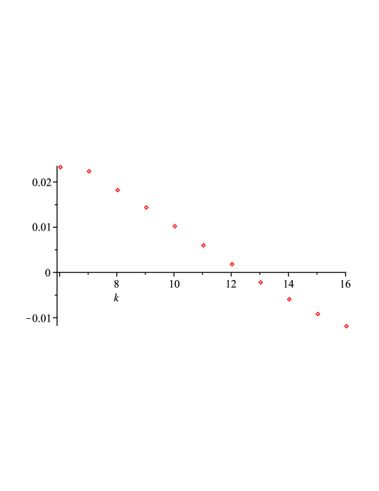
We now consider the question of whether or not $r_{c}=1$. Under Assumption A, the radius of convergence of $J(r)$ can be at most $r_{c}$, so that the Taylor coefficients of $J(r)$, or of $(r-r_{0})J(r)$, must grow (for large $k$) at least as fast as $r_{c}^{-k}$. Figure 1 shows the latter coefficients for $k=6,\ldots,16$; there is no sign of exponential growth, suggesting that $r_{c}=1$.

Figure 1: The Taylor coefficients of $(r-r_{0})J(r)$.

Accepting provisionally that $r_{c}=1$ we now ask about the form of the singularity in $J(r)$ there. The heuristic formula (1.2) suggests that

$$J(r)\sim 1/4-\gamma\,e^{-a/(1-r)}\quad\hbox{ for $r\lessapprox 1$},\qquad\gamma,a>0,$$ (3.2)

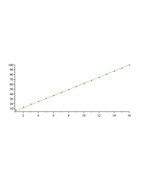
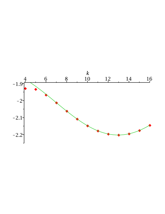
so that $(1/4-J(r))^{-1}\sim\gamma^{-1}\exp(a/(1-r))$. To verify the consistency of this ansatz we observe (see Appendix D) that the Taylor coefficients of $\exp(a/(1-r))$ grow as ${\rm const}\cdot k^{-3/4}e^{2\sqrt{ak}}(1+o(1))$. With $u_{k}$ the Taylor coefficients of $(1/4-J(r))^{-1}$ we use the function Statistics[Fit] in Maple to obtain a fit (also shown in Figure 2) over the range $7\leq k\leq 16$ of the form $u_{k}\sim A_{1}\sqrt{k}+B_{1}\log k+C_{1}$ with $A_{1}=2.82$, $B_{1}=-0.495$, and $C_{1}=0.116$; the residual standard deviation in the fit, that is, the square root of the ratio of the residual sum of squares to the number of degrees of freedom (here 7), is 0.0002, quite small. The value of $A_{1}$ is consistent with the value $a\approx 2$ which we discuss below; B1, C1 (and higher terms if sought) are more sensitive to corrections to the exact type of the singularity, to other singularities, etc.

Figure 2: A plot of $\log^{2}u_{k}$ together with a straight line fit, where the $u_{k}$ are the Taylor coefficients of $(1/4-J(r))^{-1}$.

To explore (3.2) further we consider

$$X(r)=\log[(r-r_{0})(1/4-J(r))].$$ (3.3)

If (3.2) holds then $X$ will have a simple pole at $r=1$, which by itself would lead to a Taylor series for $X$ with all coefficients equal to $-a$; due to the presence of other singularities we would of course expect such constancy at best asymptotically. A singularity of $X$ for $|r|<1$ would lead to exponentially growing coefficients, while other singularities on the unit circle would modify the asymptotic form.

The Taylor coefficients $x_{k}$ of $X$ are plotted in Figure 3. There is no sign of exponential growth, again suggesting that $r_{c}=1$ (and more generally that $J(r)\neq 1/4$ for $|r|<1$). At a first approximation one has $x_{k}\approx-2$, which is consistent with (3.2) with $a\approx 2$. Overall, we believe that this analysis gives good support for the conclusion that $r_{c}=1$ and that $j(r)$ has a singularity of the general form (3.2) at $r=r_{c}=1$.

Somewhat more speculatively, one may in fact obtain a more detailed hypothesis for the singularity structure of $J(r)$. Figure 3 suggests an oscillatory behavior rather than constancy for the $x_{k}$. Using the function Statistics[Fit] in Maple we obtain a very good fit (also shown in Figure 3) to a function of the form $x(k)=A+B\cos(C(k-D))$, with

$$A=-2.00922,\quad B=0.193059,\quad C=0.260931,\quad D=0.919233,$$ (3.4)

over the range $7\leq k\leq 16$. The residual standard deviation is 0.00025, about one hundredth of one percent of the typical value being fitted.

Figure 3: The Taylor coefficients of $\log[1/4-(r-r_{0})J(r)]$, together with the curve $A+B\cos(C(k-D))$ with parameters given by (3.4) .

The function $\hat{X}(r)$ with Taylor series given exactly by $\sum_{k=0}^{\infty}x(k)r^{k}$ is

$$\hat{X}(r)=\frac{A}{1-r}+\frac{B[\cos CD-r\cos(C(D+1))]}{1-2r\cos C+r^{2}},$$ (3.5)

with simple poles at $r=1$ and $r=e^{\pm iC}$. This suggests that one may well-approximate $X(r)$ by the function $Y(r)$ whose Taylor series agrees asymptotically with that of $\hat{X}(r)$ but has the same first 16 terms as does that of $X(r)$,

$$X(r)\approx Y(r):=\hat{X}(r)+\sum_{k=0}^{16}(x_{k}-x(k))r^{k},$$ (3.6)

and correspondingly approximate

$$J(r)\approx K(r):=\frac{1}{4}-\frac{e^{Y(r)}}{r-r_{0}}.$$ (3.7)

By construction the first 16 coefficients in the power series for $K(r)$ agree with those of $J(r)$; the $17^{\rm th}$ coefficient is negative, suggesting that the alternation of sign noted in Table 1 breaks down at this point.

One must again treat this analysis with caution; certainly for example the exact values of $A,\ldots,D$ depend on the range of indices $k$ over which the fit is performed.

Remark 3.1.

One can attempt a similar analysis of the power series for the densities $\rho_{i}(r)$ for small values of $i$, whose coefficients are also given in Appendix B. It is natural to guess that, near $r=1$, $\rho_{i}$ would have a decomposition similar to (3.2): $\rho_{i}(r)=\rho^{\rm reg}_{i}(r)+\rho^{\rm sing}_{i}(r)$, with $\rho^{\rm reg}_{i}$ regular at $r=1$ and $\rho^{\rm sing}_{i}$ having an exponential singularity $e^{-A/(1-r)}$. (Since the current is given by $j(r)=r\langle\eta_{0}(1-\eta_{1})\rangle=\langle\eta_{i}(1-\eta_{i+1})\rangle$, $i\neq 0$, where the expectation is taken in any NESS with maximal current, occurrence of the exponential singularity of (3.2) in the current implies that it must occur in densities and/or in the two-body correlation functions.) The key to the analysis of the current, however, was that we knew (or could hypothesize) that the regular part of the current at $r=1$ was precisely $1/4$, and could therefore isolate the singular part for further study through the definition (3.3) of $X(r)$. On the other hand, while we know that $\rho_{i}(1)=\rho^{\rm reg}(1)=0.5$, it appears that the derivatives of $\rho_{i}$ (or equivalently of $\rho^{\rm reg}_{i}$) at $r=1$ are nonzero, and we have not been able either to determine reliably any terms beyond the constant one in the expansion of $\rho^{\rm reg}_{i}$ around $r=1$ or to isolate $\rho^{\rm sing}_{i}$ so that its behavior could be studied.

4 A solvable semi-infinite model

We would like to understand the convergence of the finite volume current $j^{\rm ring}_{L}(r)$ (or $j_{L}^{\alpha,\beta}(r)$) as $L\to\infty$, with particular attention to the behavior in the complex $r$ plane, and for this purpose consider a semi-infinite system in which this behavior can be determined completely, using the work of Derrida, Evans, Hakim, and Pasquier [3]. To obtain this model we begin with the open system as described in Section 1, with $\beta=1$, and then replace the portion of this system lying to the left of the distinguished bond by a reservoir of particles, so that the site immediately to the left of this bond is always full. Now we study the portion of the system to the right of the bond; particles enter this system from the left at rate $r$ and (in the finite system, now of $L$ sites) exit on the right at rate 1. The current in this system is an upper bound for that in the original model [6, 2].

The system may alternatively be viewed as a symmetrized TASEP on ${\mathbb{Z}}$ [10]: the configurations are assumed to be symmetric under the joint action of the reflection $i\to 1-i$ exchange of particles and holes, and the dynamics are such that a transitions occur simultaneously on symmetrically located bonds, at rate $r$ on the bond from 0 to 1, which is invariant under the symmetry, and at rate 1 on all others. Note that if the symmetry condition is satisfied by the initial condition then it is preserved by the dynamics. In this language the model is again related to a last passage percolation model, a discrete-time version of which was studied in [15].

The current $j^{\text{s-i}}_{L}$ in this system is computed in [3]:

$$j^{\text{s-i}}_{L}(r)=\frac{rQ^{\text{s-i}}_{L-1}(r)}{Q^{\text{s-i}}_{L}(r)},$$ (4.1)

where the polynomial $Q^{\text{s-i}}_{L}$ has order $L$ and is given explicitly by

$$Q^{\text{s-i}}_{L}(r)=\sum_{j=0}^{L}\frac{L+1-j}{L+1}\binom{L+j}{L}r^{j},$$ (4.2)

and implicitly through the recursion

$$Q^{\text{s-i}}_{L-1}(r)=(1-r)Q^{\text{s-i}}_{L}(r)+\frac{1}{L+1}\binom{2L}{L}r^{L+1},\quad L\geq 1,$$ (4.3)

with $Q^{\text{s-i}}_{0}(r)=1$. It follows from (4.3) that

$$j^{\text{s-i}}_{L}(r)=r(1-r)+O(r^{L+2}).$$ (4.4)

It is further shown in [3] that

$$j^{\text{s-i}}(r)=\lim_{L\to\infty}j^{\text{s-i}}_{L}(r)=\begin{cases}r(1-r),&\hbox{if $0\leq r<1/2$,}\\ 1/4,&\hbox{if $r\geq 1/2.$}\end{cases}$$ (4.5)

Thus the critical value of $r$ in this model, $r^{\text{s-i}}_{c}=1/2$, is very different from $r_{c}$, and moreover the behavior of $j^{\text{s-i}}(r)$ near $r^{\text{s-i}}_{c}$ is very different from that conjectured in (3.2) for $j(r)$ near $r_{c}$.

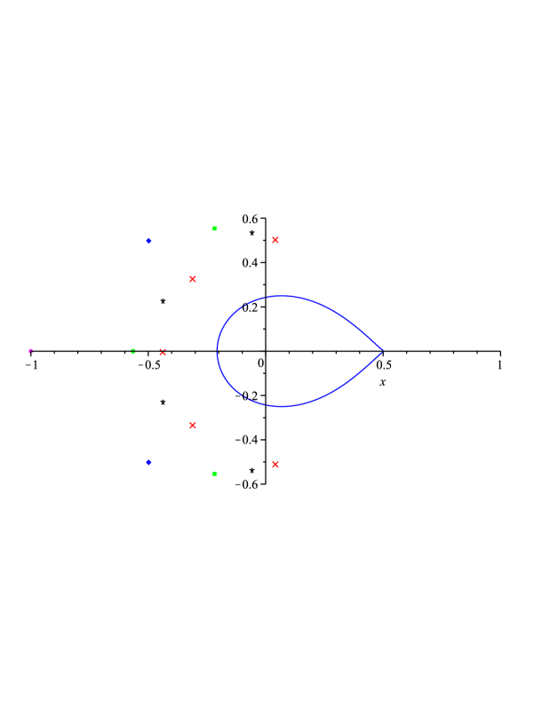
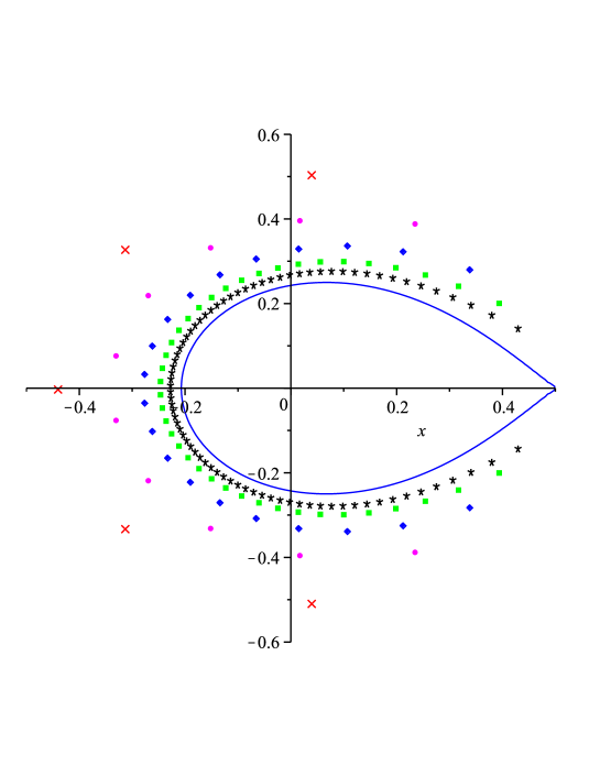
The analysis which leads to (4.5) can be carried out also in the complex $r$ plane. The simple closed curve $\Gamma$ defined by $|r(1-r)|=1/4$, ${\mathop{\rm Re}}\;r\leq 1/2$, divides the plane into an interior region $\Omega_{1}$ and an exterior region $\Omega_{2}$; see Figure 4. Then for complex $r$,

$$j^{\text{s-i}}(r)=\lim_{L\to\infty}j^{\text{s-i}}_{L}(r)=\begin{cases}r(1-r),&\hbox{if $r\in\Omega_{1}$,}\\ 1/4,&\hbox{if $r\in\Omega_{2}.$}\end{cases}$$ (4.6)

We see also that $|j^{\text{s-i}}(r)|$ is continuous on $\Gamma$.

The mechanism for the convergence (4.6) can be explored since the zeros of the polynomial $Q^{\text{s-i}}_{L}$ can be obtained and plotted numerically for reasonably large systems; this “Lee-Yang” approach to non-equilibrium systems was introduced in [16] and has been applied to the open TASEP in [17]. The zeros appear to fall on a smooth curve which approaches $\Gamma$ as $L$ increases; the limiting curve $\Gamma$ and the density of the zeros were computed in [17]. The distance of the zeros from $\Gamma$ decreases approximately as $1/L$, and the rightmost (complex conjugate) zeros lie at a distance of order approximately $1/\sqrt{L}$ from the point $r=1/2$. See Figure 4, which plots the curve $\Gamma$ and the zeros of $Q^{\text{s-i}}_{L}$ for $L=5$, $10$, $20$, $40$, and $80$. These zeros are of course poles of $j^{\text{s-i}}_{L}$. Note from (4.4) that there is no trace of these singularities in the first $L+1$ terms of the power series for $j^{\text{s-i}}_{L}$; rather they are hidden in the $O(r^{L+2})$ remainder.

Figure 4: Zeros of the denominator $Q^{\text{s-i}}_{L}(r)$: The symbols are: $L=5$, red cross, $L=10$, magenta circle; $L=20$; blue diamond; $L=40$, green square; $L=80$, black star. The solid line is the curve $\Gamma=\{r\mid|r(1-r)|=1/4\}$.

Comparison of the models: We now want to describe a certain parallelism between the blockage and semi-infinite models, and to suggest that this may extend to some properties which can be established for the latter but not for the former. To make specific comparisons, we will consider the finite-volume version of the blockage model to be that on the ring, but similar conclusions hold for the interval.

Before discussing this parallelism, however, we note a key difference between the models: in the representation (4.1) of $j^{\text{s-i}}_{L}$ the numerator and denominator are polynomials in $r$ of degree $L$, while if for the finite-volume blockage model we write

$$j^{\rm ring}_{L}(r)=\frac{P^{\rm ring}_{L}(r)}{Q^{\rm ring}_{L}(r)},$$ (4.7)

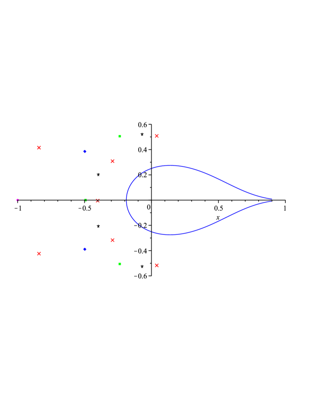
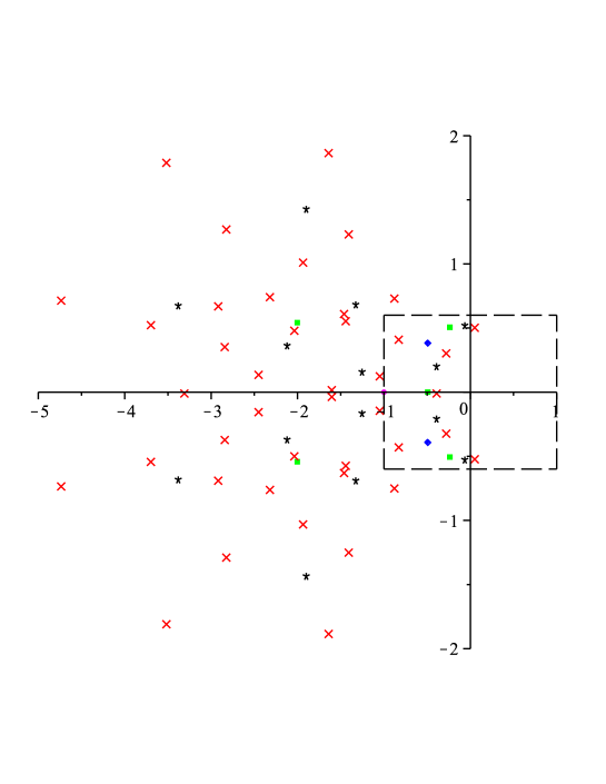
with $P^{\rm ring}_{L}(r)$ and $Q^{\rm ring}_{L}(r)$ polynomials, then the degree of $P^{\rm ring}_{L}$ and $Q^{\rm ring}_{L}$ grows exponentially with $L$. This of course makes it difficult to carry out computations in the complex $r$ plane for the blockage model similar to those described above for the semi-infinite model. To illustrate the difficulty we have calculated $Q^{\rm ring}_{L}(r)$ for $L\leq 5$; the degrees of these polynomials are $1$, $2$, $5$, $14$, and 42 for $L=1$, 2, 3, 4, and 5, respectively. Their zeros are shown in Figure 5, and one may compare the complexity of this figure with the relative simplicity of Figure 4.

Figure 5: Zeros of the denominator $Q^{\rm ring}_{L}(r)$: $L=1$, magenta circle; $L=2$; blue diamond; $L=3$, green square; $L=4$, black star; $L=5$, red cross. An expanded view of the dashed square is given in Figure 6(b).

We next note two particular similarities between the models.

1. In each model the coefficient of order $k$ of the Taylor series for the finite volume current, $j^{\rm ring}_{L}(r)$ or $j^{\text{s-i}}_{L}(r)$, is independent of $L$ for $L\geq k$; compare (2.3) and (4.4). The parallelism is not complete: if we pass to the power series obtained from the $L$-independent terms we obtain in the semi-infinite model just a polynomial of degree two, $r(1-r)$, and in the original model the rather complicated function $J(r)$ studied in Section 2, but for our present purposes we will ignore this distinction.

2. Although we have emphasized above that the singularity structure of $j^{\rm ring}_{L}(r)$ is much more complicated than that of $j^{\text{s-i}}_{L}(r)$, there nevertheless are similarities. To see this, consider the two plots of Figure 6. Here we show:

   • for the semi-infinite model (Figure 6(a)) the zeros of $Q^{\text{s-i}}_{L}$ for $L=1,2,3,4,5$, as well as the limiting curve $\Gamma$;

   • for the blockage model (Figure 6(b)), only the zeros of $Q^{\rm ring}_{L}$, $L=1,2,3,4,5$, which lie near the origin; for the window chosen, exactly $L$ zeros appear for $Q^{\rm ring}_{L}$ (as for the semi-infinite model) except for $L=5$, for which two extra zeros, farthest from the origin, also appear. Also shown is a possible limiting curve discussed below.

   The similarity of these sets of zeros is clear.

Figure 6(a)

Figure 6(b)

Figure 6: Zeros of the denominator of the current for the semi-infinite model (a) and the blockage system on the ring (b), for $N=1$, magenta circle; $N=2$; blue diamond; $N=3$, green square; $N=4$, black star; $N=5$, red cross. Also shown are the limiting curve $\Gamma$ for the semi-infinite model and an approximation to the conjectured limiting curve $\hat{\Gamma}$ of (4.8).

This parallelism suggests the following possible behavior for the blockage model:

• Some subset of the zeros of $Q^{\rm ring}_{L}$ converge as $L\nearrow\infty$ to a curve $\hat{\Gamma}$ somewhat similar to $\Gamma$. The simplest hypothesis is that $\hat{\Gamma}$ is determined by the relation

  $$|J(r)|=\frac{1}{4},$$ (4.8)

  in parallel with the definition of $\Gamma$. The curve shown in Figure 6(b) was obtained by numerical solution of $K(r)=1/4$, where $K(r)$ is the approximation to $J(r)$ defined in (3.7).

• In the interior of the curve $\hat{\Gamma}$, $J(r)$ is analytic and the finite volume current $j^{\rm ring}_{L}(r)$ converges to $J(r)$ as $L\nearrow\infty$. In particular, Assumption A of Section 2 is valid.

• The behavior of $J(r)$ outside $\hat{\Gamma}$ has no direct connection with the behavior of the finite volume current $j^{\rm ring}_{L}(r)$ there.

This suggested behavior is not sufficiently well founded to be called a conjecture, but we hope that it may be a guide to further investigation.

Acknowledgments: We have greatly benefited from discussions with M. Bramson and B. Derrida, and also thank M. den Nijs, T. Seppäläinen, V. Sidoravicius, and H. Spohn for helpful conversations and correspondence. J.L.L and E.R.S. thank the IHES for hospitality. The work of OC was supported in part by NSF Grants DMS-0600369 and DMS-1108794, and that of JLL in part by NSF Grant DMR-1104501 and AFOSR grant FA9550-10-1-0131.

Appendix A Agreement of $J_{\rm max}(r)$ and $j(r)$

In this appendix we sketch a proof that the current $j(r)$ defined in Section 1 is identical to the current $J_{\rm max}(r)$ introduced in [8] and shown there to be continuous, showing that $j(r)$ is continuous.

Consider three versions of the 1-d TASEP process: $\eta_{t}$ is a process on ${\mathbb{Z}}$ with initial configuration $\eta_{0}(i)=1$ if $i\leq 0$, $\eta_{0}(i)=0$ if $i>0$; $\zeta_{t}$ is likewise a process on ${\mathbb{Z}}$ but with arbitrary initial configuration $\zeta_{0}$, and $\tau_{t}$ is a process on the interval $\{-L+1,\ldots,L\}$ with entry and exit rates 1 and with initial configuration the restriction of $\eta_{0}$ to this interval. Transitions in these processes occur at rate 1 on all bonds except $\{0,1\}$, where the rate is $r$; moreover, the dynamics are coupled so that the same Poisson clock on each bond controls transitions in each process, and the clocks on $\{-L,-L+1\}$ and $\{L,L+1\}$ control also the entry and exit, respectively, of particles in the $\tau$ process.

Suppose now that $\mu$ is a measure on $\{0,1\}^{{\mathbb{Z}}}$ which is invariant for the TASEP dynamics with the rates given above and has (maximal) current $j(r)=r\langle\eta_{0}(1-\eta_{1})\rangle_{\mu}$. (For the sake of precision we define also $j^{1,1}_{L}(r)=r\langle\eta_{0}(1-\eta_{1})\rangle_{\mu^{1,1}_{L}}$ with $\mu^{1,1}_{L}$ the invariant measure for the open system.) Let $N_{\eta}(t)$ be the number of particles that cross the special bond in the $\eta$ process between times $0$ and $t$, with $N_{\zeta}(t)$ and $N_{\tau}(t)$ defined similarly. From the coupling one sees easily that $N_{\tau}(t)\geq N_{\eta}(t)\geq N_{\zeta}(t)$ for all $t$ and all $\zeta_{0}$, so that for $t>0$,

$${\mathbb{E}}{\left[\frac{N_{\tau}(t)}{t}\right]}\geq{\mathbb{E}}{\left[\frac{N_{\eta}(t)}{t}\right]}\geq{\mathbb{E}}{\left[\frac{\langle N_{\zeta}(t)\rangle_{\mu}}{t}\right]},$$ (A.1)

where ${\mathbb{E}}{\left[\cdot\right]}$ denotes the average over the dynamics and in $\langle N_{\zeta}(t)\rangle_{\mu}$ the initial configuration $\zeta_{0}$ is averaged over $\mu$. But also

$$j(r) = {\mathbb{E}}{\left[\frac{\langle N_{\zeta}(t)\rangle_{\mu}}{t}\right]},\quad t>0,$$ (A.2)

$$j^{1,1}_{L}(r) = \lim_{t\to\infty}{\mathbb{E}}{\left[\frac{N_{\tau}(t)}{t}\right]},$$ (A.3)

We show below that $\lim_{t\to\infty}{\mathbb{E}}{\left[N_{\eta}(t)/t\right]}=J_{\rm max}(r)$; with (1.1) and (A.1)–(A.3) this completes the proof.

For $n\geq 1$ let $T_{n}$ be the time of the $n^{\rm th}$ crossing of the $\{0,1\}$ bond by a particle in the $\eta_{t}$ process. It is shown in [8] that $\kappa(r)=\lim_{n\to\infty}T_{n}/n$ exists almost surely and is constant. The current $J_{\rm max}$ is defined to be $1/\kappa(r)$, so that $J_{\rm max}(r)=\lim_{n\to\infty}n/T_{n}$ a.s. It is easy to see that $N_{\eta}(t)\to\infty$ and so $T_{N_{\eta}(t)}\to\infty$ a.s. as $t\to\infty$; from this and the inequalities

$$\frac{N_{\eta}(t)+1}{T_{N_{\eta}(t)+1}}-\frac{1}{T_{N_{\eta}(t)+1}}<\frac{N_{\eta}(t)}{t}\leq\frac{N_{\eta}(t)}{T_{N_{\eta}(t)}},$$ (A.4)

we see that $\lim_{t\to\infty}N_{\eta}(t)/t=J_{\rm max}$ a.s. We complete the proof by verifying that the family of random variables $\{N_{\eta}(t)/t\mid t\geq 1\}$ is uniformly integrable, that is, that

$$\lim_{c\nearrow\infty}\,\max_{t\geq 1}\,{\mathbb{E}}\left[\frac{N_{\eta}(t)}{t}\chi_{\bigl{\{}\frac{N_{\eta}(t)}{t}\geq c\bigr{\}}}\right],$$ (A.5)

where $\chi_{S}$ denotes the characteristic function of the set $S$.

Note first that $T_{n}\geq S_{n}$, where $S_{n}$ is the sum of $n$ independent exponential random variables of mean 1 (these can be taken, for example, to be the variables $Y_{i,i}$, $1\leq i\leq n$, of [8]). Then for $c\geq 2$, and using $T_{N_{\eta}(t)}\leq t$, we have

$${\mathbb{E}}\left[\frac{N_{\eta}(t)}{t}\chi_{\{N_{\eta}(t)\geq ct\}}\right] = \sum_{n=2}^{\infty}{\mathbb{E}}\left[\frac{n}{t}\chi_{\{N_{\eta}(t)=n\}}\chi_{\{n\geq ct\}}\right]$$ (A.6)

$$\leq \sum_{n=2}^{\infty}{\mathbb{E}}\left[\frac{n}{S_{n}}\chi_{\{n\geq cS_{n}\}}\right].$$

Now $n/S_{n}$ is gamma-distributed with density $n^{n}x^{n-1}e^{-nx}/(n-1)!$, so that, using $n!\geq n^{n}e^{-n}$, we have

$${\mathbb{E}}\left[\frac{n}{S_{n}}\chi_{\{n\geq cS_{n}\}}\right]\leq\frac{n^{n}}{(n-1)!}\int_{0}^{1/c}x^{n}\,dx\leq\frac{e^{n}}{c^{n+1}},$$ (A.7)

and (A.5) follows from (A.6) and (A.7).

Appendix B Tables of coefficients

We give in Table 1 below the coefficients in the power series (3.1) for the current $J(r)$, to order 16, and in Table 2 the coefficients in the series

$$\rho_{i}(r)=\sum_{k=0}^{\infty}d_{ik}r^{k}$$ (B.1)

for $\rho_{i}$, up to order $16-i$, for $i=1,\ldots,5$. In Table 1 we report the values to 20 decimal places. We believe that these digits are reliable because in our computation of $c_{0},\ldots c_{15}$ the first 24 digits obtained were stable under increase in the system size (this test is not available for $c_{16}$). For $c_{0},\ldots c_{13}$ a check for stability under change in the precision used in the program found the same reliability.

$k$	$c_{k}$		$k$	$c_{k}$
0	0.00000000000000000000		9	0.09696668201649961665
1	1.00000000000000000000		10	-0.05607405058503243547
2	-1.50000000000000000000		11	0.04033294103506195933
3	1.18750000000000000000		12	-0.02482314806701423240
4	-0.77889901620370370370		13	0.01477809455732788252
5	0.52961027553406380931		14	-0.01328263357536883488
6	-0.32787247554422253211		15	0.00277198065020739725
7	0.22700745336484005616		16	-0.00936905520626202337
8	-0.13514784111152134747

Table 1: The coefficients of the power series $J(r)$.

$k$	$d_{1k}$	$d_{2k}$	$d_{3k}$	$d_{4k}$	$d_{5k}$
0	0.00000000	0.00000000	0.00000000	0.00000000	0.00000000
1	1.00000000	1.00000000	1.00000000	1.00000000	1.00000000
2	-0.75000000	-0.68750000	-0.65625000	-0.63671875	-0.62304688
3	0.45312500	0.40075231	0.37939743	0.36763019	0.36002612
4	-0.32345016	-0.31775049	-0.32035731	-0.32441081	-0.32884964
5	0.19113754	0.16723143	0.15934419	0.15807536	0.16042006
6	-0.13508488	-0.13527025	-0.14002291	-0.14544675	-0.15090756
7	0.08218276	0.07251374	0.06758191	0.06440565	0.06221118
8	-0.05412219	-0.05222456	-0.05418729	-0.05745286	-0.06108373
9	0.03743811	0.03658774	0.03602396	0.03505521	0.03382992
10	-0.01961547	-0.01492080	-0.01314674	-0.01296838	-0.01376695
11	0.01873543	0.02252206	0.02556734	0.02764994	0.02887908
12	-0.00544623	0.00051738	0.00480082	0.00795647
13	0.01025427	0.01536259	0.02003591
14	-0.00040069	0.00489313
15	0.00558944

Table 2: The coefficients $d_{ik}$ of the power series $\rho_{i}=\sum_{k}d_{ik}r^{k}$.

Appendix C The value of $r_{0}$

As observed in Section 3, the power series for the current suggests the existence of a pole at some value $r_{0}\approx-1.5$. In this appendix we attempt to determine an accurate value for $r_{0}$ by two independent methods.

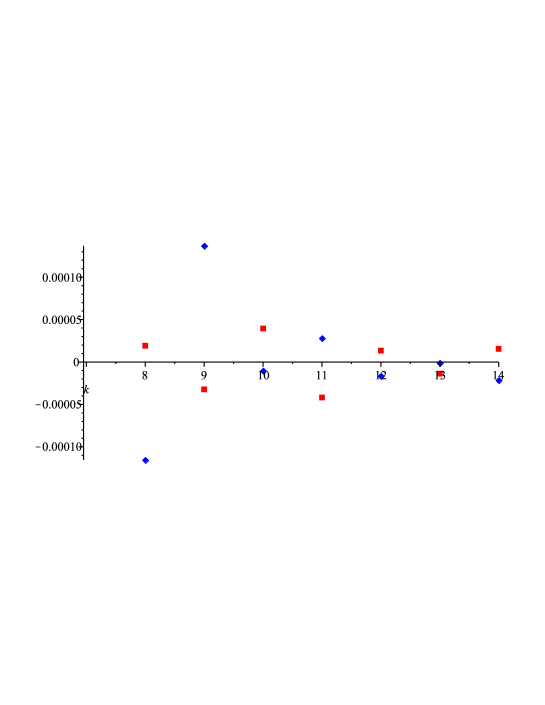
Method 1. We let $W(r)=(r-r_{0})\,J(r)$ and compute, for various values of $r_{0}$, the Taylor polynomial $W_{16}(r)=\sum_{k=0}^{16}w_{k}r^{k}$. The oscillation in the coefficients $w_{k}$ should be minimized for the correct value of $r_{0}$; to emphasize the oscillation we compute the second difference $\hat{w}_{k}=w_{k+2}-2w_{k+1}+w_{k}$ as well as $\tilde{w}(k)$, the least-squares linear fit to $\hat{w}_{k}$ over the range $k=8\ldots 14$, and plot in Figure 7 the difference $\hat{w}_{k}-\tilde{w}(k)$ for $r_{0}=-1.5435$ and $-1.5440$. The oscillations clearly change sign over this range of $r_{0}$ and will be minimized at some intermediate value.

Figure 7: The difference $\hat{w}_{k}-\tilde{w}(k)$ for $r_{0}=3.5435$ (red squares) and $r_{0}=3.5440$ (blue diamonds).

Method 2. Consider the function $V(r)=1/(1/4-J(r))$, which has a zero at $r=r_{0}$ and for which we expect a singularity at $r=1$, due both to the vanishing of the denominator and to the (hypothetical) exponential singularity of $J(r)$ suggested in (1.2). The fractional linear transformation

$$u=u(r)=\left(\frac{1-r_{1}}{r_{1}}\right)\frac{r}{1-r},\quad\Leftrightarrow\quad r=r(u)=\frac{r_{1}u}{1+r_{1}(1-u)},$$ (C.1)

with $r_{1}=-1.5$, leaves the origin unchanged, carries $r=r_{1}$ to $u=1$, and moves the singularity at $r=1$ as far away as possible, to $u=\infty$. We write $\hat{V}(u)=V(r(u))$ and find that $\hat{V}_{16}(u)$ has one zero $u_{0}$ very near to $u=1$, corresponding to $r_{0}=r(u_{0})=1.5437$, and that all other zeros are a distance at least 1.39 from $u=0$. The value of $r_{0}$ found by this procedure is independent, to very high precision, of the choice of $r_{1}$ in (C.1) for $-3\leq r_{1}\leq-1$.

Thus the two methods above give good agreement and suggest that $r_{0}\in[-1.540,-1.535]$. We take $r_{0}=-1.5437$ and expect this value to be accurate within an error of $\pm 0.0005$.

Appendix D Asymptotics of Taylor coefficients

In this section we find the large $k$ asymptotic behavior of the coefficients $b_{k}$ in the Maclaurin series

$$e^{a/(1-r)}=\sum_{k=0}^{\infty}b_{k}r^{k},\ \ |r|<1,$$ (D.1)

where $a$ is a positive number. We have

$$b_{k}=\frac{1}{2\pi i}\oint_{\mathcal{C}_{1}}\frac{e^{a/(1-s)}}{s^{k+1}}ds=\oint_{\mathcal{C}_{2}}e^{-a/t-(k+1)\ln(1+t)}dt,$$ (D.2)

with $\mathcal{C}_{1}$ a circle of radius $R<1$ centered at $0$, traversed anticlockwise, and $\mathcal{C}_{2}=-1+\mathcal{C}_{1}$. The saddle points of $-a/t-(k+1)\ln(1+t)$ are:

$$t_{+}=\frac{a+\sqrt{a(a+4k+4)}}{2(k+1)}\ \text{and}\ t_{-}=\frac{a-\sqrt{a(a+4k+4)}}{2(k+1)}.$$ (D.3)

The steepest variation path homotopic to $\mathcal{C}_{2}$ and passing through $t_{-}$ is an analytic curve orthogonal at $t_{-}$ to the real line. The saddle point method applied at $t=t_{-}$ gives

$$b_{k}={\rm const}\cdot k^{-3/4}e^{2\sqrt{ak}}(1+o(1))\ \text{as}\ k\to\infty.$$ (D.4)

References

- [1] T. M. Liggett, Interacting particle systems, Springer-Verlag, New York, 1985.
- [2] T. M. Liggett, Stochastic interacting systems: contact, voter and exclusion processes, Springer-Verlag, Berlin, 1999.
- [3] B. Derrida, M. R. Evans, V. Hakim, and V. Pasquier, Exact solution of a D asymmetric exclusion model using a matrix formulation. J. Phys. A 26, 1493–1517 (1993).
- [4] G. Schütz and E. Domany, Phase transitions in an exactly soluble one-dimensional asymmetric exclusion model. J. Stat. Phys. 72, 277-296 (1993).
- [5] S. Janowsky and J. L. Lebowitz, Finite size effects and shock fluctuations in the asymmetric simple exclusion process. Physical Review A 45, 618-625 (1992).
- [6] S. Janowsky and J. L. Lebowitz, Exact Results for the Asymmetric Simple Exclusion Process with a Blockage. Journal of Statistical Physics 77, 35-51 (1994).
- [7] P. Covert and F. Rezakhanlou, Hydrodynamic limit for particle systems with nonconstant speed parameter. J. Stat. Phys. 88, 383–426 (1997).
- [8] T. Seppäläinen, Hydrodynamic profiles for the totally asymmetric exclusion process with a slow bond. J. Stat. Phys. 102, 69–96 (2001).
- [9] K. Johansson, Shape Fluctuations and Random Matrices. Communications in Mathematical Physics 209, 437–476 (2000).
- [10] M. Prähofer and H. Spohn, Current fluctuations for the totally asymmetric simple exclusion process. In Progress in Probability 51: In and Out of Equilibrium, ed. V. Sidoravicius, Birkh user, 2002.
- [11] M. Ha, J. Timonen, and M. den Nijs, Queuing transitions in the asymmetric simple exclusion process. Phys. Rev. E 68, 056122 (2003).
- [12] T. Hwa and T. Natterman, Disorder induced depinning transition. Phys. Rev. B 51, 455–469 (1995).
- [13] V. Beffara, V. Sidoravicius, and M. E. Vares, Randomized polynuclear growth with a columnar defect. Probab. Theory Relat. Fields 147, 565–581 (2010).
- [14] V. Sidoravicius, private communication.
- [15] J. Baik and E. M. Rains, Symmetrized random permutations. In MSRI Publications 40: Random Matrix Models and Their Applications, ed. P. Bleher and A. Its, Cambridge, 2001.
- [16] P. F. Arndt, Lee-Yang theory for a nonequilibrium phase transition. Phys. Rev. Lett. 84, 814–817 (2000).
- [17] R. A. Blythe and M. R. Evans, Lee-Yang Zeros and Phase Transitions in Nonequilibrium Steady States. Phys. Rev. Lett. 89, 080601 (2002).