A Rogue-Langmuir-type traveling wave continuous solution to nonlinearly dispersive Schrödinger equation using a polynomial expansion scheme

Abstract

In this paper, traveling wave solutions to the nonlinearly dispersive Schrödinger equation are given in the case of one-dimensional non-relativistic electron confined to a cylindrical quantum well. Investigations gave evidence to the possibility of implementing continuous solutions for a quantum-based problem.
 
Keywords: Schrödinger equation; Non-relativistic electron, Quantum well; Boubaker Polynomials expansion scheme (BPES); Rogue-Langmuir traveling wave.

 
 
 

1 Introduction

The well-known nonlinearly dispersive Schrödinger equation [1]-[8], described as:

$$\mathrm{i}\frac{\partial u}{\partial t}+\frac{\partial^{2}\left(u\left\lvert\mspace{1.0mu}u\mspace{1.0mu}\right\rvert^{n-1}\right)}{\partial x^{2}}+\mu u\left\lvert\mspace{1.0mu}u\mspace{1.0mu}\right\rvert^{m-1}=0,$$ (1.1)

where $u$ is the unknown function which determines the probability distribution, $\mu$ is a given parameter and $m$ and $n$ are positive integers and denote the intensity of the nonlinear term. This equation arises from the research of nonlinear wave propagation in dispersive and inhomogeneous media. It has been also encountered in problems of plasma physics, hydrodynamics, self trapping of light with formation of spatiotemporal solitons, evolution of slowly varying electromagnetic field as well as early studies of pulses in optical wave fibers [5]-[12].

Exact and analytical solutions for nonlinearly dispersive Schrödinger equation have attracted considerable attention [9]-[16]. Several attempts yielded families of exact analytical solutions which were obtained using elementary functions [11]-[14].

In the present work, a polynomial expansion scheme is performed in order to obtain Rogue-Langmuir-type traveling wave solution to Eq. (1.1). This paper is organized as follows. In Section 2, the resolution protocol is presented along with the studied system patterns. In Section 3, plots of the solutions are shown ad discussed. Last section is the conclusion.

2 Resolution protocol

Schrödinger’s equation is introduced here in the case of a one-dimensional non-relativistic electron $e$- of mass $m$, moving inside a cylindrical quantum well $(C)$ of radius $R$ (Fig. 1).

Figure 1: Non-relativistic electron moving inside a cylindrical quantum well

The potential in the whole space is defined as

$$\begin{cases}V(r)=0,&r\in(0,R)\\ V(r)=\infty,&r\in(R,\infty)\end{cases}$$ (2.1)

That is to say, there is an infinitely high cylindrical infinite R-radius envelop at walls at $r=R$ and the particle is trapped in the region $r\in[0,R]$.

Schrödinger’s equation in cylindrical co-ordinate system for the non-relativistic electron in quantum well is

$$\mathrm{i}\hbar\frac{\partial u(r,t)}{\partial t}+\frac{\hbar^{2}}{2m}\frac{\partial^{2}\left(u(r,t)\left\lvert\mspace{1.0mu}u(r,t)\mspace{1.0mu}\right\rvert^{n-1}\right)}{\partial x^{2}}=V(r)u(r,t)\left\lvert\mspace{1.0mu}u(r,t)\mspace{1.0mu}\right\rvert^{m-1}.$$ (2.2)

Since it is the matter of finding a Rogue-Langmuir traveling wave solution of Eq. (1.1), we introduce the wave variable $\theta$, so that

$$x=-\frac{\mathrm{i}\hbar}{p}\theta+Et.$$ (2.3)

We have consequently:

$$\begin{cases}\frac{\partial}{\partial x}(\cdot)&=-\frac{\mathrm{i}\hbar}{p}\frac{\partial}{\partial\theta}(\cdot)\\ \frac{\partial^{2}}{\partial^{2}x}(\cdot)&=-\frac{\mathrm{i}\hbar}{p}\frac{\partial^{2}}{\partial^{2}\theta}(\cdot)\\ \frac{\partial}{\partial t}(\cdot)&=-\frac{\mathrm{i}\hbar}{pE}\frac{\partial}{\partial\theta}(\cdot)\\ \end{cases}$$ (2.4)

so that Eq. (1.1) becomes, for $n=2$ and $m=3$:

$$\begin{cases}\left(\frac{p}{\hbar}\right)^{2}\frac{d^{2}f(\theta)}{d\theta^{2}}+\left(\frac{E}{\hbar}+\left(\frac{p}{\hbar}\right)^{2}\right)f(\theta)-V(r)f^{3}(\theta)=0&\\ f(\theta)=u(x,t)\exp\left(-\frac{\mathrm{i}}{\hbar}(px-Et)\right)=u(x,t)e^{-\theta}&{}\textstyle\end{cases}$$ (2.5)

Since $\left\lvert\mspace{1.0mu}u\mspace{1.0mu}\right\rvert^{2}$ represents the probability of finding the electron anywhere, we have the trivial condition $\left\lvert\mspace{1.0mu}u\mspace{1.0mu}\right\rvert\equiv 0$ for $r\in(R,\infty)$. According to the BPES principles, the expression of the unknown term of the traveling wave solution is proposed as following

$$f(\theta)=\frac{1}{2N_{0}}\sum^{N_{0}}_{k=1}\widetilde{\xi_{k}}\cdot B_{4k}(\theta\mu_{k}),$$ (2.6)

where $B_{4k}$ are the $4k$-order Boubaker polynomials, $\mu_{k}$ are $B_{4k}$ minimal positive roots [17]-[36], $N_{0}$ is a prefixed integer, and $\widetilde{\xi_{k}}(k=1,\ldots,N_{0})$ are unknown pondering real coefficients.

The main advantage of these formulations Eq. (2.6) is the fact of verifying boundary conditions, at the earliest stage of resolution protocol thanks to the properties of the Boubaker polynomials [19]-[33]:

$$\begin{cases}\sum^{N}_{q=1}B_{4q}(x)|_{x=0}&=-2N\neq 0\\ \sum^{N}_{q=1}B_{4q}(x)|_{x=\mu_{q}}&=0\\ \end{cases}$$ (2.7)

and

$$\begin{cases}\sum^{N}_{q=1}\frac{dB_{4q}(x)}{dx}|_{x=0}&=0\\ \sum^{N}_{q=1}\frac{dB_{4q}(x)}{dx}|_{x=\mu_{q}}&=\sum^{N}_{q=1}H_{q}\\ \end{cases}$$ (2.8)

with

$$H_{n}=B_{4n}(\mu_{n})=\frac{4\mu_{n}(2-\mu^{2}_{n})\sum^{n}_{q=1}B^{2}_{4q}(\mu_{n})}{B_{4(n+1)}(\mu_{n})}+4\mu^{3}_{n}.$$

Thanks to the properties expressed by Eqs. (2.7), (2.8), boundary conditions are trivially verified in advance to resolution process. Eq. (2.5) becomes, for the given potential expression in Eq. (2.1):

$$\left(\frac{p}{\hbar}\right)^{2}\sum^{N_{0}}_{k=1}\widetilde{\xi_{k}}\mu^{2}_{k}\frac{d^{2}B_{4k}(\theta\mu_{k})}{d\theta^{2}}+\left(\frac{E}{\hbar}+\left(\frac{p}{\hbar}\right)^{2}\right)\sum^{N_{0}}_{k=1}\widetilde{\xi_{k}}B_{4k}(\theta\mu_{k})=0.$$ (2.9)

The BPES solution is obtained by determining the non-null set of coefficients $\widetilde{\xi_{k}}^{\mathrm{(sol.)}}(k=1,\ldots,N_{0})$ that minimizes the absolute functional $\Omega_{N_{0}}$:

$$\Omega_{N_{0}}=\left\lvert\mspace{1.0mu}\sum^{N_{0}}_{k=1}\mu^{2}_{k}\widetilde{\xi_{k}}^{\mathrm{(sol.)}}\Lambda_{k}+\frac{1}{2N_{0}}\sum^{N_{0}}_{k=1}\widetilde{\xi_{k}}^{\mathrm{(sol.)}}\Lambda^{\prime}_{k}\mspace{1.0mu}\right\rvert$$ (2.10)

with

$$\Lambda_{k}=\frac{p^{2}}{2\hbar^{2}N_{0}}\oint_{(C)}\frac{d^{2}B_{4k}(\theta\mu_{k})}{d\theta^{2}}d\theta,\quad\Lambda^{\prime}_{k}=\frac{1}{2N_{0}}\left(\frac{E}{\hbar}+\left(\frac{p}{\hbar}\right)^{2}\right)\oint_{(C)}B_{4k}(\theta\mu_{k})d\theta.$$

Finally the solution of Eq. (2.2) is

$$u^{\mathrm{(sol.)}}(x,t)=\frac{1}{2N_{0}}\sum^{N_{0}}_{k=1}\widetilde{\xi_{k}}^{\mathrm{(sol.)}}B_{4k}\left(\frac{\mathrm{i}}{\hbar}(px-Et)\mu_{k}\right)\exp\left(-\frac{\mathrm{i}}{\hbar}(px-Et)\right)$$ (2.11)

where $x\in[0,R],t\in[0,t_{m}],t_{m}=\frac{2\pi\hbar}{E}$.

The main advantage of this solution is the fact that, oppositely to most on classical solutions [37]-[40], no quantification is imposed to the couple $(p,E)$. The solution is hence uni-modal and piecewise continuous. Moreover, convergence is obtained for moderate values of $N_{0}$, since, as mentioned above, boundary conditions were verified in advance to resolution process.

3 Solution plots and patterns

Fig. 2 shows that plots of the solution, for increasing values of $N_{0}(N_{0}=11,23,43)$, while Fig. 3 corresponds to the convergent solution modulus, obtained for $N_{0}>57$. All the solutions have been represented with $[0,1]$ and $[0,t_{m}]$ as space and time ranges, respectively.

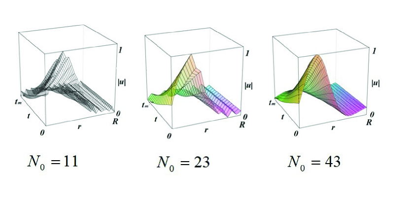
Figure 2: Solution convergence patterns(plots for $N_{0}=11,23,43$)

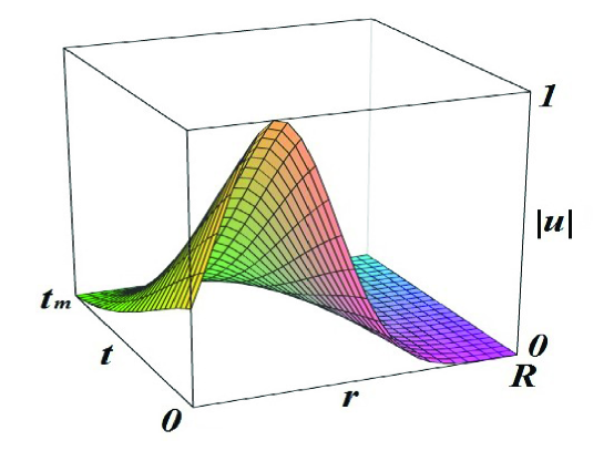
Figure 3: Solution plots for $N_{0}>57$

It may be appropriate to point out that Eq. (2.2) is derived for short amplitude quasi-stationary slow motion describing the Rogue-Langmuir pondero-motive force. Most of classical solutions, which describe a classical-type particle motion under the action of such forces, consist of linear sums of wave functions corresponding to different energies [41]. The present solution accounts for the trapping of such waves in an infinite well, and oppositely to many other results, it concentrates the electron energy into a small region near at the vicinity of the central zone (Fig. 4). This paradox can be explained by the nonlinear properties of the medium as well as the abrupt potential discontinuity at the envelope $r=R$.

Fig. 4 presents the probability distribution within the cylinder $(C)$. It monitors a typical single energy wave function having a static probability distribution.

Figure 4: Probability distribution $\left(\left\lvert\mspace{1.0mu}u\mspace{1.0mu}\right\rvert^{2}\right)$ within the cylinder $(C)$

4 Conclusion

In summary, we have proposed piecewise continuous and uni-modal Rogue-Langmuir-type traveling wave solution to the well known Schrödinger equation. The performed polynomial scheme has ensured the verification of boundary condition in advance to resolution process. The obtained solutions have been expressed in terms of wave function modulus and presented the singular advantage of imposing no quantification for both particle momentum and energy oppositely to most classical solutions. The convergence of the protocol has been discussed and enhanced.

References

- [1] T.A. Davvdova, A.I. Fishchuk, Phys. Lett. A 245: 453-459 (1998).
- [2] M. Porkolab, M.V. Goldman, Phys. Fluid 19: 872-881 (1976).
- [3] K.P. Sharma, P.K. Shukla, Phys. Rev. A 28: 1182-1185 (1983).
- [4] A.G. Litvak, A.M. Sergeev, Pisma Zh. Eksp. Teor. Fiz. 27: 549-553 (1978).
- [5] T.A. Davydova, A.I. Fishchuk, Ukrainian J. Phys. 40: 487-494 (1995).
- [6] T.A. Davydova, A.I. Fishchuk, Phys. Scripta 57: 118-126 (1998).
- [7] Y.F. Chen, C.Y. Wang, S.H. Wang, I.A. Yu, Phys. Rev. Lett. 96: 043603 (2006).
- [8] X. Wang , D. Brown, K. Lindenberg, Phys. Rev. A 37:3557-3566 (1988).
- [9] Kh.I. Pushkarov, D. I. Pushkarov, and I.V. Tomov: Opt. Quant. Electr. 11: 471 (1979).
- [10] J.M. Zhu and Z.Y. Ma, Chaos, Solitons & Fractals 33: 958 (2007).
- [11] S. Tanev and D.I. Pushkarov, Opt. Commun. 141: 322 (1997).
- [12] L. Gagnon, J. Opt. Soc. Am. A 6: 1477 (1989).
- [13] H.W. Schürmann: Phys. Rev. E 54: 4312 (1996).
- [14] Z. Birnbaum and B.A. Malomed: Physica D 237: 3252 (2008).
- [15] J. Fujioka and A. Espinosa, J. Phys. Soc. Jpn. 65: 2440 (1996).
- [16] S.L. Palacios, Chaos, Solitons & Fractals 19: 203 (2004).
- [17] A. Milgram, J. of Theoretical Biology 271: 157-158 (2011).
- [18] J. Ghanouchi, H. Labiadh and K. Boubaker, Int. J. of Heat and Technology 26: 49-53 (2008).
- [19] S. Slama, J. Bessrour, K. Boubaker and M. Bouhafs, Eur. Phys. J. Appl. Phys. 44: 317-322 (2008).
- [20] S. Slama, M. Bouhafs and K.B. Ben Mahmoud, Int. J. of Heat and Techn.26(2): 141-146 (2008).
- [21] S. Lazzez, K.B. Ben Mahmoud, S. Abroug, F. Saadallah, M. Amlouk, Current Applied Physics 9(5): 1129-1133 (2009).
- [22] T. Ghrib, K. Boubaker and M. Bouhafs, Modern Physics Letters B 22: 2893-2907 (2008).
- [23] S. Fridjine, K.B. Ben Mahmoud, M. Amlouk, M. Bouhafs, Journal of Alloys and Compounds 479(1-2): 457-461 (2009).
- [24] C. Khélia, K. Boubaker, T. Ben Nasrallah, M. Amlouk, S. Belgacem, Journal of Alloys and Compounds 477(1-2): 461-467 (2009).
- [25] K.B. Ben Mahmoud, M. Amlouk, Materials Letters 63(12): 991-994 (2009).
- [26] M. Dada, O.B. Awojoyogbe, K. Boubaker, Current Applied Physics, 9(3): 622-624(2009).
- [27] S. Tabatabaei, T. Zhao, O. Awojoyogbe, F. Moses, Int.J. Heat Mass Transfer 45: 1247-1255 (2009).
- [28] A. Belhadj, J. Bessrour, M. Bouhafs, L. Barrallier, J. of Thermal Analysis and Calorimetry 97: 911-920 (2009).
- [29] A. Belhadj, O. Onyango, N. Rozibaeva, J. Thermophys. Heat Transf. 23: 639-642 (2009).
- [30] P. Barry, A. Hennessy, Journal of Integer Sequences 13: 1-34 (2010).
- [31] M. Agida, A.S. Kumar, El. Journal of Theoretical Physics 7: 319-326 (2010).
- [32] A. Yildirim, S.T. Mohyud-Din, D.H. Zhang, Computers and Mathematics with Applications 59: 2473-2477 (2010).
- [33] A.S. Kumar, Journal of the Franklin Institute 347: 1755-1761 (2010).
- [34] S. Fridjine, M. Amlouk, Modern Phys. Lett. B 23: 2179-2182 (2009).
- [35] M. Benhaliliba, C.E. Benouis, K. Boubaker,M. Amlouk, A. Amlouk, A New Guide To Thermally Optimized Doped Oxides Monolayer Spray-grown Solar Cells: The Amlouk-boubaker Optothermal Expansivity ab in the book : Solar Cells - New Aspects and Solutions, Edited by: Leonid A. Kosyachenko, [ISBN 978-953-307-761-1, by InTech] 27-41 (2011).
- [36] H. Rahmanov, Studies in Nonlinear Sciences 2(1): 46-49 (2011).
- [37] N. Fabien II, M. Alidou, K.T. Crépin, Modulational instability in the cubic-quintic nonlinear Schrödinger equation through the variational approach. Optics Commun. 275(2): 421-428 (2007).
- [38] V.E. Zakharov, E.A. Kuznetsov, Optical solitons and quasisolitons. Sov. Phys. JETP 86: 1035-1046 (1998).
- [39] G.S. Agarwal and S.D. Gupta, Phys. Rev. A 38: 5678 (1988).
- [40] J. Fujioka and A. Espinosa, J. Phys. Soc. Jpn. 66: 2601 (1997).
- [41] M.Ya Amusia, L.V. Chernvsheva, Computation of Atomic Processes, Taylor & Francis (1997).