Reliable estimation of the column density in Smoothed Particle Hydrodynamic simulations.

Abstract

We describe a simple method for estimating the vertical column density in Smoothed Particle Hydrodynamics (SPH) simulations of discs. As in the method of Stamatellos et al. (2007), the column density is estimated using pre-computed local quantities and is then used to estimate the radiative cooling rate. The cooling rate is a quantity of considerable importance, for example, in assessing the probability of disc fragmentation. Our method has three steps: (i) the column density from the particle to the mid plane is estimated using the vertical component of the gravitational acceleration, (ii) the “total surface density” from the mid plane to the surface of the disc is calculated, (iii) the column density from each particle to the surface is calculated from the difference between (i) and (ii). This method is shown to greatly improve the accuracy of column density estimates in disc geometry compared with the method of Stamatellos. On the other hand, although the accuracy of our method is still acceptable in the case of high density fragments formed within discs, we find that the Stamatellos method performs better than our method in this regime. Thus, a hybrid method (where the method is switched in regions of large over-density) may be optimal.

1 Introduction

Smooth Particle Hydrodynamics (SPH) (Lucy, 1977; Gingold & Monaghan, 1977) is a Lagrangian technique for simulating fluid flows using a particle representation. This technique assigns each particle a mass, position and internal energy and then interpolates state variables, such as density, by “smoothing” over neighbouring particles. Gravity has been incorporated into the SPH formalism, allowing SPH to be used to simulate astrophysical fluids. However, the thermal evolution of many astrophysical systems is often governed by radiative transfer effects, in addition to hydrodynamic energy transfer. As an accurate description of a system’s thermal evolution is of vital importance in many astrophysical systems (e.g. accretion discs, stellar gas clouds) a lot of effort has recently been made to add radiative transfer to SPH (Oxley & Woolfson, 2003; Whitehouse & Bate, 2004a; Stamatellos et al., 2007; Forgan et al., 2009). Unfortunately, a full three dimensional, frequency dependent description of radiative transfer is currently computationally impossible, so simplifying assumptions have to be made.

Since SPH is a Lagrangian method, the purpose of modeling radiative transfer effects is to provide a net cooling (or heating) rate per particle as a result of radiative processes. For example, a popular choice for simulating self-gravitating discs is to use a cooling time prescription, where the radiative cooling rate $\dot{U}$ is set equal to $\frac{-U}{t_{cool}}$ where $U$ is the cooling rate per unit mass and $t_{cool}$ is simply parameterised as a prescribed multiple of the local dynamical timescale (Rice et al., 2003). Although such a description grossly oversimplifies the underlying physics, it has a very low computational cost and so simulations including approximating radiative cooling can be run without sacrificing spatial or temporal resolution. Recently, Stamatellos et al have proposed a method that improves upon the cooling time prescription without significantly increasing the computational cost (Stamatellos et al., 2007). Forgan et al extended this method to include heat transfer between particles, by combining the Stamatellos method with the flux limited diffusion (FLD) method (Forgan et al., 2009).

The Stamatellos method estimates the optical depth by assuming that the relationship between the two locally computed variables, density and gravitational potential, and the optical depth is the same as it is for a mass-weighted average of that relationship over a self-gravitating polytropic sphere. They then estimate the local cooling rate using only the local temperature and optical depth. This estimate tends to the radiative diffusion approximation at high optical depths but does not involve calculating noisy derivatives as is required in a proper implementation of radiative diffusion (Whitehouse & Bate, 2004b). The aim of such methods is not to achieve perfect agreement with the full radiative transfer equations, but to achieve an accuracy that is comparable in magnitude to the other uncertainties such as those associated with the grey approximation and the appropriate values of the frequency averaged opacity.

However, although the Stamatellos method has proved successful for modelling spherical systems, Wilkins & Clarke have shown that it can systematically underestimate the cooling in disc geometries by as much as a factor of four in the region of the mid plane, where column density estimation is critical to estimating the cooling (Wilkins & Clarke, 2012). This underestimate stems from the Stamatellos method overestimating the column density, $\Sigma$, which appears as a quadratic term in the expression for the cooling rate in the optically thick limit. An example of where radiative transfer is important to the evolution of a disc system is the study of gravitational instabilities in proto-planetary disc. The cooling time prescription has been used to study these discs in great detail, but a more accurate description of the cooling in such systems is necessary to improve our understanding of these gravitational instabilities (Forgan et al., 2011).

In this paper we propose a variation on the Stamatellos method for calculating the cooling rate for the special case of disc geometries, by improving the estimate of the column density in this case. Our method still only requires the use of local quantities, already calculated by the gravitational and hydrodynamic codes and as such remains computationally inexpensive. The paper is organized as follows. In section 2, we describe our new method in detail. In section 3, we test our method on a series of discs for which all quantities of interest can be obtained analytically or semi-analytically. In section 4 we test our method on realistic disc simulations that have been evolved long enough to either fragment or reach marginal stability. Finally, section 5 summarises our conclusions.

2 The Method

For a typical astrophysical disc, most of the cooling occurs at the disc’s surface. Therefore, we assume that the greatest contribution to the radiative cooling of a particle within such a disc comes from energy radiated vertically out of the disc, rather than along the optically thick mid-plane. Assuming this is true, we estimate the cooling rate of each particle using the optical depth, $\tau$, along a vertical path from the particle to the disc’s surface. The true optical depth is given by $\tau=\int\kappa(z)\rho(z)dz$. In order to avoid evaluating this costly integral we make the approximation that $\tau=\kappa\int\rho dz=\kappa\Sigma$, where $\Sigma$ is the column density to the surface and $\kappa$ is the local opacity. Next, we follow Stamatellos et al in defining the cooling rate per unit mass to be:

$$\dot{U}=\frac{\sigma(T^{4}-T_{0}^{4})}{\tau\Sigma+\widetilde{\kappa}^{-1}}$$ (1)

where, $\tau$ is the optical depth to the surface of the disc, $\sigma$ is the Stefan Boltzman constant, $\Sigma$ is the column density from the particle to the surface of the disc and $\widetilde{\kappa}$ is the local Planck-mean opacity. The $T_{0}$ term is a background temperature below which particles are not allowed to cool.

In the regime where $T^{4}\gg T_{0}^{4}$, we find that there are two limiting cases. The first limiting case is the optically thin limit, where $\tau\Sigma\ll\widetilde{\kappa}^{-1}$. In this limit, the cooling simply reduces to

$$\dot{U}=\sigma T^{4}\widetilde{\kappa}$$ (2)

which is just the cooling rate for an isolated particle, in an environment with opacity $\widetilde{\kappa}$. However, note that this is not a good approximation to the cooling rate per unit mass for an optically thin layer on top of an optically thick disc, which is a commonly encountered situation. Fortunately, in practice the thermodynamics of such layers are often controlled by the background temperature, $T_{0}$.

In the optically thick limit, $\tau\Sigma\gg\widetilde{\kappa}^{-1}$ and equation 1 becomes

$$\dot{U}=\frac{\sigma T^{4}}{\Sigma\tau}$$ (3)

which is an approximation to the commonly used diffusion approximation (see Mihalas (1970), section 2.3). To see why, consider the optically thick limit, in which the radiative flux is given by:

$$F=-\frac{4}{3\kappa\rho}\nabla\sigma T^{4}$$ (4)

and the corresponding cooling rate per unit mass as:

$$\dot{U}=\frac{1}{\rho}\nabla.F$$ (5)

If integration and differentiation over $z$ are replaced by simple multiplication and division by an effective vertical scale height, $H$, then an expression of the same form as 3 is obtained.

$$\dot{U}=\frac{1}{\rho}\nabla.F\approx\frac{\sigma T^{4}}{\kappa\Sigma^{2}}\approx\frac{\sigma T^{4}}{\tau\Sigma}$$ (6)

Note that because $\dot{U}\propto\Sigma^{-2}$, any inaccuracy in the column density to the surface, $\Sigma$, will have a large effect on the inaccuracy of the cooling rate.

$\Sigma$ is calculated in a three step process. Firstly, an estimate of the column density between the particle and the mid-plane is obtained. This is done using only the vertical component of the gravitational acceleration, which is already calculated by the simulation making this step essentially “free” from a computational standpoint. Secondly, a total surface density map (i.e. map of column density from the mid-plane to the surface) is computed. Finally, the column density to the surface is calculated by subtracting the column density to the mid-plane from the total surface density.

2.1 Estimating the column density to the mid-plane

We estimate the column density of each particle to the mid-plane using the approximation:

$$g_{z}=-\frac{GMz}{r^{3}}-4\pi G\Sigma^{\prime}sign(z)$$ (7)

where $M$ is the mass of the central star, $r=\sqrt{x^{2}+y^{2}+z^{2}}$ and $\Sigma^{\prime}$ is the column density between the point at height $z$ and the mid-plane. The first term in this expression is the contribution from the central star, whereas the second term comes from assuming that the disc is infinite in extent and has the same vertical density structure everywhere. In reality, there will be further corrections to this expression due to radial variation in the disc’s vertical density structure and its finite extent (see e.g. Appendix of Bertin & Lodato (1999).) However, we expect these contributions to be small in most cases, an assumption that will be investigated in detail in section 3.

As the gravitational acceleration, $g_{z}$, is already calculated by the simulation for every particle, we can re-arrange equation (7) to estimate the column density from the particle to the mid-plane.

$$\Sigma^{\prime}=-\frac{sign(z)}{4\pi G}\left(g_{z}+\frac{GMz}{r^{3}}\right)$$ (8)

2.2 Constructing a surface density map

In order to calculate the cooling, we need to know the column density between the particle and the surface of the disc, and therefore the column density to the mid-plane, estimated in equation (8) above, has to be subtracted from an estimate of the total column density. This map can be calculated in a number of different ways, discussed at length in Appendix B and the section below. In this paper, we calculate the map by projecting all particles onto the mid-plane and then interpolating for each particle from a density map evaluated at the location of a subset of particles ($10\%$). The surface density for the remaining 90% of points are interpolated when needed. Once obtained, we can estimate the column density to the surface, $\Sigma$, by:

$$\Sigma=\Sigma_{map}-\Sigma^{\prime}$$ (9)

2.3 Computational efficiency

The construction of a total surface density map, has the potential to be computationally expensive. The potentially expensive aspect of this step is the estimation of the surface density at each particle from the particle positions and masses, projected onto the mid plane. There already exists an extensive literature devoted to solving this problem, which we will not attempt to reproduce in detail here. Importantly, the choice of method for estimating density involves a trade off between accuracy, computational speed and the ability to recover sharp density gradients (see (Ferdosi et al., 2011) for a discussion of these trade-offs in the context of astronomical datasets).

SPH density estimation methods give excellent accuracy, but a high computational cost ($O(N^{2})$, e.g. the “DEDICA” method in Ferdosi et al. (2011))). At the other extreme, grid based methods offer excellent computational efficiency ($O(N)$), but with reduced accuracy (e.g. the “MBE” method in Ferdosi et al. (2011)). The method we use here (describe in appendix B) is intermediate in complexity between these two extremes and is very similar to the “kNN” method described in Ferdosi et al. (2011), which has $O(NlogN)$ scaling.

The computational cost of any of the above method can be reduced, at the cost of “smoothing out” the density distribution, by evaluating the density at a subset of points and then interpolating the values at the particle locations.

It is important to note that the calculation of a total surface density map is a two-dimensional version of the calculation of the three-dimensional density of each particle, which must be performed by any SPH code. As such, even in the worst case scenario this step will be no more expensive than the 3D density calculation already performed by the code. Furthermore, as there is little gain in calculating the surface density to greater accuracy than the other sources of error in our method (see discussion below), a computationally cheaper density estimator can usually be used.

2.4 Sources of inaccuracy

The accuracy of this method can be affected by a number of different factors. Each of these potential sources of error will be tested independently in Section 3.

i) The gravitational force calculation in self-gravitating SPH codes does not simply consist of summing pairwise interactions. In particular, the usual gravitational force is typically “softened” for small separations and distant particles are grouped together in a ‘tree’ structure, e.g. an oct-tree (Barnes & Hut, 1986). How aggressively particles are grouped and the extent of the gravitational softening is controlled by the user. As our method relies on the gravity estimated from the tree code, inaccuracies in the gravitational force may propagate in our method also.

ii) The discrete realisation of a given density distribution may produce accelerations that differ from those produced by a continuous density field since quantising the density distribution inevitably introduces “clumpiness”, which affects the resulting gravitational acceleration. Note that this error decreases with increasing resolution. The gravitational softening mentioned above also mitigates this effect.

iii) No physical disc is really an infinite slab of constant height, with density structure depending only on $z$. Deviations from this structure will obviously influence the accuracy of our method.

iv) Any inaccuracy in our map of surface densities $\Sigma_{map}$ will lead to inaccuracies in our final estimate of $\Sigma$. This inaccuracy will arise from a combination of interpolation error (as the map is only calculated for 10% of particles) and error due to the calculation of the surface density itself.

To quantify the size of these relative errors, we note that effects i)-iii) produce errors in the estimate of $\Sigma^{\prime}$, while iv) produces errors in $\Sigma_{map}$. We represent the size of these errors as $\delta\Sigma^{\prime}$ and $\delta\Sigma_{map}$, respectively. We then see that the relative error in our estimate of $\Sigma$ is:

$$\delta\left(\frac{\Sigma_{estim}}{\Sigma}\right)=\pm\frac{\sqrt{\delta\Sigma^{\prime 2}+\delta\Sigma_{map}^{2}}}{|\Sigma|}$$ (10)

Since $\Sigma$ is always smallest at large $z$, it follows that the fractional inaccuracy of our estimate is generally worst far from the mid-plane.

3 Analytic tests

As outlined in the previous section, there are a number of possible sources of inaccuracy in our column density estimate. These are: inaccuracies in the gravitational tree code, the quantization of a continuous system, the “infinite slab” approximation and inaccuracy of the surface density map.

In this section we construct a series of discs for which the gravitational acceleration, density and column density can be calculated analytically or semi-analytically. As described in Appendix A, these discs have power law density profiles between adjustable inner and outer radii, with a Gaussian variation of density with $z$ at each radius. The scale height of this Gaussian is adjusted so that it corresponds to the hydrostatic equilibrium profile of a locally isothermal non-self gravitating disc where the temperature is a power law function of radius. Because we are given a continuous, analytic density distribution, we can integrate it semi-analytically to calculate the resulting vertical component of the gravitational acceleration (equation 20). Furthermore, we can analytically determine the gravitational acceleration for the continuous density distribution under the infinite slab approximation (equation 7 without the term due to the star, where $\Sigma^{\prime}$ is given by equation 23). We also calculate the vertical component of gravitational acceleration using the oct-tree on the discretized distribution. We will henceforth refer to the gravitational acceleration calculated by integration of the continuous density distribution as the “continuous gravitational acceleration” and the value calculated using the oct-tree as the “oct-tree gravitational acceleration”. Combining these three estimates of $g_{z}$, we can independently test the sources of error identified in section 2.4. We also test the accuracy of our total surface density map by comparing it to the analytic value given by 23.

We emphasise that these discs do not represent realistic physical conditions that would result from the steady state evolution of accretion discs, but are designed to test our method for calculating the column density. As such, many of these discs will have non-uniform values of the Toomre Q parameter (Toomre, 1964), significantly different from unity and would change significantly if allowed to evolve with time.

The properties of our analytic discs are summarised in Table 1. In each case the density structure (Equation 14) corresponds to a hydrostatic structure of uniform temperature with mid-plane density scaling as $R^{-0.5}$. In running the simulations, typical parameters for the tree gravity were used (adaptive gravitational softening on the SPH smoothing length $h$, Barnes & Hut opening angle threshold of 0.3).

Parameter	Thin Disc	Thick Disc	Small Disc	High resolution
$H/R$	$0.025\sqrt{R/R_{i}}$	$0.76\sqrt{R/R_{i}}$	$0.025\sqrt{R/R_{i}}$	$0.025\sqrt{R/R_{i}}$
$\frac{R_{o}-R_{i}}{R_{o}}$	0.95	0.95	0.33	0.95
$N$	$10^{5}$	$10^{5}$	$10^{5}$	$5*10^{5}$

Table 1: The relevant properties for the gravitational force and column density, for different analytic disc geometries. $H/R$ is the aspect ratio of the disc, given as a function of cylindrical radius, $R_{o}$ and $R_{i}$ are the disc’s outer and inner radii and $N$ is the number of particles in the simulation. All discs are run with $q=M_{*}/M_{disc}=0.1$.

3.1 Varying scale heights

We first test how the accuracy of our method depends on disc thickness, where thickness is measured by $H/R$ and $H$ is the scale height of the disc. We consider a thin disc with $0.025<H/R<0.11$ and a thick disc with $0.76<H/R<3.4$.

Figures 1 and 3 show the inaccuracy in the vertical component of gravitational acceleration due to making the continuous density distribution (equation 14) discrete and demonstrate that, as expected, the errors are highest in thinner discs, particularly close to the disc mid-plane where any given particle is most affected by the “lumpy” nature of its environment (see Figures 2 and 4). The effect is exacerbated by the fact that $g_{z}\rightarrow 0$ in the densest parts of the disc, so the relative errors are largest here. Note that such quantization errors are reduced by increasing the resolution (see section 3.2).

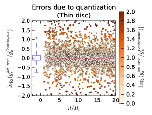
Figure 1: The log2 ratio of the vertical component of the oct-tree and continuous gravitational accelerations, as a function of cylindrical radius for a subset of 5000 particles in the ‘thin disc’ calculation ($H/R=0.025\sqrt{R/R_{i}}$). The boxplot on the left of the plot shows the distribution of errors. The box bounds the central 50% of particles (the edges are the 25% and 75% percentiles), the red line is the median and the whiskers mark the 5% and 95% percentiles.

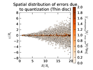
Figure 2: The locations of the particles with errors in vertical component of the gravitational acceleration colour coded as in Figure 1.

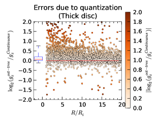
Figure 3: The log2 ratio of the vertical component of the oct-tree and continuous gravitational accelerations, as a function of cylindrical radius for a subset of 5000 particles in the ‘thick disc’ calculation ($H/R=0.76\sqrt{R/R_{i}}$). The boxplot represents the distribution of errors on this plot (see Figure 1 for explanation).

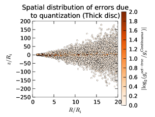
Figure 4: The locations of the particles with errors in vertical component of the gravitational acceleration colour coded as in Figure 3.

Next we investigate the inaccuracy in the gravitational acceleration due to use of the infinite slab approximation. Figure 5 show that this error is small for the thin disc, with most points being accurate to within 50% of the expected analytic value. Figure 7 shows that the accuracy of this approximation breaks down significantly in the thick disc limit. Note that this disc has been chosen to test the thick disc limit and does not represent a realistic physical situation. Figures 6 and 8 show a strong trend towards greater inaccuracy where the disc is thickest, since it is at large $z$ that particles ‘see’ the gravitational influence of radial gradients in the disc. The accuracy also decreases at the disc’s edges where the finite nature of disc has the largest effect.

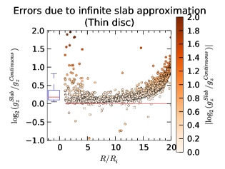
Figure 5: The log2 ratio of the vertical component of the gravitational acceleration calculated using the infinite slab approximation to the “continuous” value of the same quantity is plotted as a function of cylindrical radius for a subset of 5000 particles in the ‘thin disc’ calculation ($H/R=0.025\sqrt{R/R_{i}}$). The boxplot represents the distribution of errors on this plot (see Figure 1 for explanation).

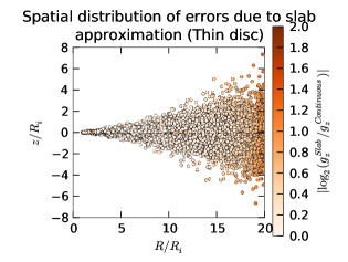
Figure 6: The locations of the particles with errors in the vertical component of the gravitational acceleration due to the infinite slab approximation colour coded as in Figure 1.

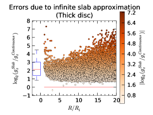
Figure 7: The log2 ratio of the vertical component of the gravitational acceleration calculated using the infinite slab approximation to the “continuous” value of the same quantity is plotted as a function of cylindrical radius for a subset of 5000 particles in the ‘thick disc’ calculation ($H/R=0.76\sqrt{R/R_{i}}$). The boxplot represents the distribution of errors on this plot (see Figure 1 for explanation).

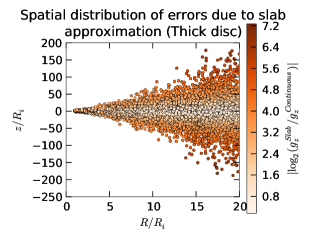
Figure 8: The locations of the particles with errors in vertical component of the gravitational acceleration colour coded as in Figure 7

Figures 9 and 10 test the accuracy of the total surface density map for the thin and thick discs, i.e. we here compare the result of interpolating the column density map obtained by sampled measurements of the projected particle distribution with the analytic value. It is clear that the accuracy is relatively insensitive to disc thickness and that most points are accurate to within a few 10s of %, with a median accuracy of $\sim 10\%$ for both discs.

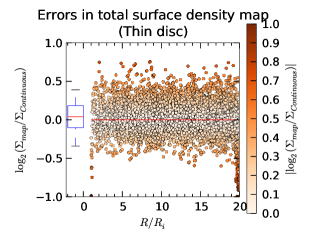
Figure 9: The log2 ratio of the calculated total surface density map to the known analytic values is shown as a function of radius for 5000 particles from the ‘thin disc’ simulation. The boxplot represents the distribution of errors on this plot (see Figure 1 for explanation).

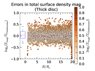
Figure 10: The log2 ratio of the calculated total surface density map to the known analytic values is shown as a function of radius for 5000 particles from the ‘thick disc’ simulation. See Figure The boxplot represents the distribution of errors on this plot (see Figure 1 for explanation).

Overall, we find that the accuracy of our estimation of the column density to the surface is controlled by errors in determining the column density to the mid-plane, rather than by errors in the total surface density. The main source of the error in determining the column density to the mid-plane depends on disc thickness (and resolution, see 3.2): thin discs are dominated by discreteness effects whereas in thick discs the accuracy of the infinite slab approximation is the limiting factor.

3.2 Effect of resolution

On theoretical grounds, we expect that the error due to quantisation will roughly depend on the “extra” acceleration imparted on a particle by its neighbours. Given that all particles are identical, the mass of each particle is given by $m=M_{disc}/N$, where $N$ is the number of particles in the simulation. Furthermore, the mean particle separation, $\lambda$, will scale roughly as $\lambda\propto N^{-1/3}$ in a three-dimensional environment. Therefore, we expect the inaccuracy due to quantization to scale as:

$$\frac{Gm}{\lambda^{2}}\propto\frac{1}{N^{1/3}}$$ (11)

This effect will be mitigated by the inclusion of gravitational softening, which for a typical SPH simulation will modify gravity so the effect of the quantized particles becomes:

$$\frac{Gm}{(\lambda+\varepsilon)^{2}}$$ (12)

where $\varepsilon$ is typically set to the SPH smoothing length $h$ and $h$ is given by,

$$\rho h^{3}=\nu^{3}m$$ (13)

where $\nu$ is a numerical parameter usually set to 1.2. Combining equations 12 and 13 we see that the inclusion of gravitational softening does not change the $N^{-1/3}$ dependence of the quantization error, it merely decreases it by a factor of $1/(1+\nu)^{2}\sim 0.25$, compared to no gravitational softening.

In order to validate this predicted dependence on resolution, we repeat the thin disc simulation with 5 times as many particles ($5*10^{5}$). The two runs are compared in Figure 11, which shows that inaccuracy decreases as $N$ increases. We calculate the median relative error for both the high and low resolution simulations and find they have a ratio of $\sim 1.6$. Comparing this with equation 11, which predicts a decrease in error $\approx 5^{1/3}=1.7$, we see that our simulations are consistent with our theoretical predictions. All other comparisons have not been shown as they are essentially unchanged with resolution.

We see that for both our $N=10^{5}$ and $N=5*10^{5}$ runs, the error in column density estimate to the mid-plane is dominated for most particles by the inaccuracy of the infinite slab approximation (compare boxplots in Figure 11 with that in Figure 5) rather than by (resolution dependent) errors in computing $g_{z}$. Considering the region at $R/R_{i}\sim 16$ (where $H/R\sim 0.1$ in the thin disc, a value typical of protostellar discs) we can estimate (using the above $N^{-1/3}$ scaling of discreteness errors) that $N$ would have to be reduced to of order $10^{4}$ before discreteness errors dominated. Such a low value of $N$ would never be employed in a hydrodynamic calculation in any case, since it would imply that the smoothing length was larger than the disc’s vertical scale height (see Lodato & Clarke (2011) and references therein). We therefore conclude that our method of estimating the column density to the mid-plane imposes no extra resolution requirements on the code.

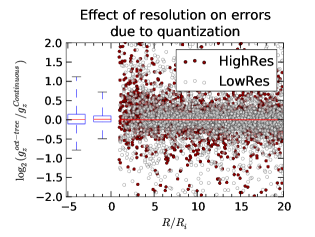
Figure 11: The log2 ratio of the vertical component of the oct-tree to the continuous gravitational acceleration for a subset of 5000 particles as a function of cylindrical radius in the ’thin disc’ calculation ( $H/R=0.025\sqrt{R/R_{i}}$) at two different resolutions ($10^{5}$ and $5*10^{5}$ particles). The left and right boxplots show the low and high resolution data respectively. The boxplots represents the distribution of errors on this plot (see Figure 1 for explanation).

3.3 Other parameters: disc mass and radial extent

The accuracy of our method is independent of the ratio of the disc mass to central object mass since the gravitational contribution due to the star is not used by our method. Changing the radial extent of the disc means that edge effects affect the accuracy of the infinite slab approximation - for example, we found that a radially restricted disc (with fractional width of $\sim 0.33$ compared with $\sim 0.95$ in the simulations discussed above) increased such errors by a factor of a few.

Generally, the infinite slab approximation is very accurate for most particles in the simulation, with 90% of particles being accurate to within a factor of 2 and over 50% of particles accurate to within a few 10s of percent. Although the inaccuracy is acceptable, we find that the infinite slab approximation slightly over-estimates the gravitational acceleration in a systematic way. Furthermore, the approximation does worst at the edges of the disc (both radially and vertically), where the deviation from an infinite slab is most obvious.

The accuracy of the total surface density map produced by our method is high, higher even than the accuracy of the infinite slab approximation, which is already very good. As such, we do not expect the total surface density map to be a significant source of error in any application.

3.4 Accuracy of the column density to the surface estimate.

Having dissected the various sources in error in calculating total surface densities and column densities to the mid-plane, we can understand the over-all accuracy of our determination of $\Sigma$ (the column density from each particle to the surface) which is to be used in the calculation of optical depths and cooling rates. Figures 12 and 13 show the relative error in $\Sigma$ (the column density from the particle to the surface), and the spatial distribution of these errors.

It is evident that the over-all accuracy is good (most particles are accurate to within a factor 2) and that the largest errors are found at large $z$. This is to be expected since for particles close to the mid-plane, the column density to the surface is controlled by the total surface density whose accuracy is of order $10\%$, regardless of the accuracy of determination of the column density to the mid-plane. At high $z$, the column density to the surface is obtained by the subtraction of two quantities of similar magnitude and the result is particularly sensitive to errors in determining the column density to the mid-plane (which, at large $z$, derive from the breakdown of the infinite slab approximation).

In practice, however, inaccuracies at high $z$ may be irrelevant to the computation of the cooling rate according to equation 1. This is because once the disc enters the optically thin regime, the cooling rate according to equation 1 is in any case independent of optical depth.

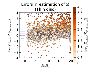
Figure 12: The relative error in $\Sigma$ (the column density to the surface from a particle) is plotted for a subset of 5000 particles as a function of cylindrical radius in the ’thin disc’ calculation ($H/R=0.025\sqrt{R/R_{i}}$). The boxplot represents the distribution of errors on this plot (see Figure 1 for explanation).

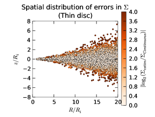
Figure 13: The locations of the particles with errors in $\Sigma$ (the column density to the surface from a particle) colour coded as in Figure 12.

4 Application to realistic discs

Up until now we have focused on evaluating our approximation in discs for which the column density could be analytically determined, rather than those that represent the outcome of realistic disc evolution. If our method is to be of any use, it is important that it is accurate not only in idealised problems, but in “real world” simulations. To provide such a test, we evaluate our method on a disc simulation kindly provided by Ken Rice and detailed in Section 3 of (Forgan et al., 2011) (Simulation 1, Table 1). Briefly, the disc was evolved using SPH with radiative cooling implemented using the method describe in (Forgan et al., 2009). The disc was constructed using $5*10^{5}$ particles distributed between 10 AU and 50 AU with a surface density profile $\Sigma\propto R^{-3/2}$. The disc to star mass ratio, $q$, was set to $0.25$. The simulation was run for 27 outer rotation periods, which was long enough for the disc to develop spiral structures and settle into marginal stability ($Q\sim 1$), where radiative cooling was matched by heat generated through gravitational instabilities.

Unlike the analytic discs, we cannot evaluate the effects of quantization and the infinite slab approximation separately. Therefore, we test our method by comparing our estimated column densities to the mid-plane and the surface, to those obtained using a counting method described in Appendix C.

Figure 14 shows a comparison of the gravity based estimates of the column density to the mid-plane and the results of the counting method. Even though this comparison includes inaccuracies from both the infinite slab approximation and the quantization of the disc, the overall accuracy remains extremely high. In fact, over 90% of particles agree to within a factor of two, with most particles agreeing to within a few 10s of percent. Furthermore, Figure 15 shows that those particles with high inaccuracy are located in surface layers where they are unlikely to affect calculations of the cooling rate.

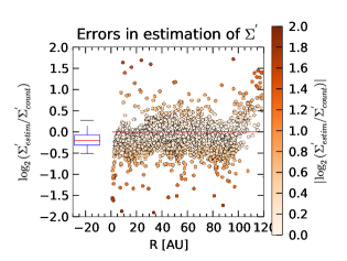
Figure 14: The log2 ratio of $\Sigma^{\prime}$ (the column density between a particle and the mid-plane) calculated using our method and by direct counting for a subset of 5000 particles as a function of cylindrical radius for the ‘marginally stable’ disc (Simulation 1, (Forgan et al., 2011)). The boxplot represents the distribution of errors on this plot (see Figure 1 for explanation).

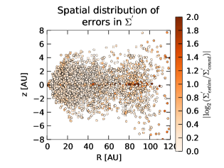
Figure 15: The locations of the particles with errors in $\Sigma^{\prime}$ colour coded as in Figure 14.

Figure 16 shows the accuracy of the column density to the surface, $\Sigma$, obtained by subtracting $\Sigma^{\prime}$ from $\Sigma_{map}$. As expected, the use of our total surface density map to infer column density to the surface does not significantly increase the error. The spatial distribution of the errors, shown in Figure 17, show that the inaccuracy in our method only becomes significant in the optically thin region, where it is unimportant for our calculation of the cooling rate.

For comparison, the column densities to the surface estimated by the Stamatellos et al (Stamatellos et al., 2007) method are also shown in black in Figure 16. The discrepancy is less large than that found by Wilkins & Clarke (2012) (who used a thinner disc), but is significant nonetheless. Specifically, the Stamatellos method has a larger dispersion than our method and has a systematic offset of around a factor of 4. As can be seen in equation 6, the cooling rate depends on $\Sigma$ quadratically in the optically thick limit, so this factor 4 discrepancy gives an order of magnitude under-estimate of the cooling rate.

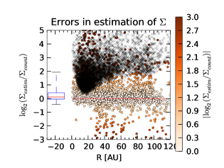
Figure 16: The log2 ratio of $\Sigma$ (the column density between a particle and the surface) calculated using our method and by direct counting, for a subset of 5000 particles as a function of cylindrical radius for the ‘marginally stable’ disc (Simulation 1, (Forgan et al., 2011)). The black crosses show the log2 ratio of estimating $\Sigma$ using the Stamatellos et al method (Stamatellos et al., 2007) and the same value calculated by direct counting. The boxplot represents the distribution of errors on this plot (see Figure 1 for explanation).

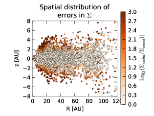
Figure 17: The locations of the particles with errors in $\Sigma$ colour coded as in Figure 16.

For simulations involving spiral structures, such as the one considered here, it is important to be able to resolve the differences between the cooling rates in the spiral arms and outside of them. In Figure 18 we plot our estimated total surface density map next to an “exact map” and show that the essential features of the disc are still clearly visible. This implies that our method would be able to correctly distinguish between on arm and off arm cooling. We find that $\delta\Sigma/\Sigma<0.05$ for $R<20$ and then rises steadily to a mean value of $\sim 0.2$. Comparing this with Figure 18, we conclude that we can easily resolve density perturbation for which $\delta\Sigma/\Sigma>0.05$. Resolving smaller density perturbations could be achieved by increasing from 10% the number of points at which the surface density map is calculated.

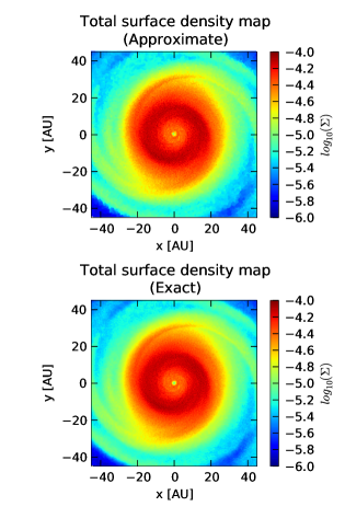
Figure 18: The two heat maps show the total surface density inferred by the method used to estimate the column density (top) and an “exact” counting method (bottom). The colour bars show the mapping between total surface density and colour used in this plot (log scale).

4.1 Fragmented discs

While the above section shows that our method works well for self-gravitating discs in marginal stability (where heating due to gravitational turbulence is balanced by cooling), it does not test its ability to recover the cooling of fragments if they form. To test this, we consider a fragmented disc, which is originally 50 AU in size, with a disc to star mass ratio of .1, which has been evolved for  5 outer rotational periods (data provided by Peter Cossins). Figure 19 shows a total surface density map calculated using our method, which clearly shows the presence of several fragments.

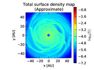
Figure 19: A heat map showing the total surface density estimate for the fragmented disc described in section 4.1. The colour bar shows the mapping between total surface density and colour on a log scale.

To test our methods ability to recover the column density within a fragment, we focus the rest of our analysis on the .25 AU around the fragment at  (-40,15) (see Figure 19). We calculate the column density to the surface ($\Sigma$) for each particle in this region and compare it to the column density obtained using the same counting method as used in section 4 above. The results of this comparison are shown in Figure 20. As with Figure 16, we also include the column density estimated by the Stamatellos method for comparison (the black dots in the figure). Figure 20 shows that our method does not perform as well as the Stamatellos method in reproducing the column density within fragments. Although our method is still accurate to within a factor of two for the majority of the particles, there is a systematic trend for our method to over-estimate the column density, while the Stamatellos method shows no systematically bias here, unlike the rest of the disc. Figure 21 shows that as before, the lowest accuracy points are still located at high $z$, where the column density is less important to estimating the cooling rate.

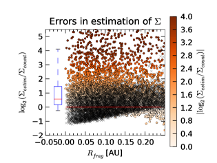
Figure 20: The log2 ratio of $\Sigma$ (the column density between a particle and the surface) calculated using our method and by direct counting, for all particles within .25 AU of the fragment located at (-40,15) in Figure 19, as a function of cylindrical radius from the centre of the fragment. The black crosses show the log2 ratio of estimating $\Sigma$ using the Stamatellos et al method (Stamatellos et al., 2007) and the same value calculated by direct counting. The boxplot represents the distribution of errors on this plot (see Figure 1 for explanation).

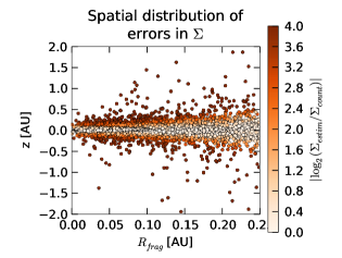
Figure 21: The locations of the particles with errors in $\Sigma$ colour coded as in Figure 20 as a function of cylindrical radius $R_{frag}$ and $z$ from the centre of the fragment.

It is perhaps unsurprising that our method performs less well within a fragment, as fragments have a roughly spherical geometry where the infinite slab approximation is likely to break down. The same reasoning explains why the Stamatellos method does so well here, as it is known to perform well for problems with a spherical geometry.

The calculation of our total surface density map provides a mechanism for combining the advantages of our method with those of the Stamatellos method in fragmented discs. That is, the Stamatellos method can be used to estimate $\Sigma$ within the fragments and our method can be used everywhere else, where a fragment can be defined to be a region where the total surface density exceeds the average value by two orders of magnitude. Indeed, this is the exact definition used to identify fragments in many studies of fragmenting discs (e.g. Forgan et al. (2011)). Such a scheme would combine the advantages of the two methods and provide an estimate of the column density without systematic bias for the entirety of the fragmented disc and may be optimal when the cooling within fragments is an important consideration.

5 Conclusion

In this paper we have presented a new method for efficiently and accurately estimating the cooling in disc geometries. To achieve this, our method estimates the column density between each particle and the surface of the disc, via estimates of the column density to the mid-plane and the total surface density. We verify the accuracy of our column density estimation (and hence our cooling rates) by comparison with discs for which the analytic form of the column density can be calculated. We test our method on a realistic proto-planetary disc simulation, that has been evolved for long enough to reach marginal stability and develop a typical spiral structure. Finally, we test our method on a fragmented disc and find that our method does not perform as well as the Stamatellos method within the fragments, due to the locally spherical geometry. We suggest that this shortcoming can be resolved by using the Stamatellos method only within regions of extremely high density (i.e. the fragments). We find throughout our tests that the accuracy of our method remains high (i.e. typical errors of order a few tens of per cent) and conclude that it is ideally suited for use in problems that depend on an accurate estimate of the cooling rate in disc geometries.

6 Materials & Methods

In the interests of reproducibility and transparency, all code and data used in performing this work have been made freely available online.

The generation of initial conditions and the code used to perform the analyses described in this paper can be found at https://bitbucket.org/constantAmateur/disccolumndensity. See the readme file in this repository for further details. The gravitational acceleration for the analytic discs was calculated using a modified version of GADGET-2.0 (Springel, 2005), which can be obtained from https://bitbucket.org/constantAmateur/gadgetoutputgravaccel. Converting of initial conditions to/from ascii files was done using the code from https://bitbucket.org/constantAmateur/easyic.

The data from the spiral simulation used in section 4 were provided by Ken Rice (Forgan et al., 2011). The fragmented disc used in section 4.1 were provided by Peter Cossins and Giuseppe Lodato (unpublished). Both are made available at https://bitbucket.org/constantAmateur/disccolumndensity with the original authors’ permission.

7 Acknowledgements

We would like to thank Ken Rice for providing the simulation data used is section 4. We would also like to thank Giuseppe Lodato and Peter Cossins for providing the simulation data use in section 4.1. Finally, we thank an anonymous referee for valuable comments that have improved the paper. Matthew Young gratefully acknowledges the support of a Poynton Cambridge Australia Scholarship.

Appendix A The analytic column density

Consider a disc with density profile ($\rho(R,z)$) given by:

$$\rho=\frac{M_{d}(\alpha_{\rho}+2)}{2\pi\left(R_{o}^{\alpha_{\rho}+2}-R_{i}^{\alpha_{\rho}+2}\right)}R^{\alpha_{\rho}}\frac{e^{-z^{2}/2H^{2}}}{\sqrt{2\pi H^{2}}}$$ (14)

This corresponds to a disc of mass $M_{d}$, inner and outer radii $R_{i}$ and $R_{o}$ and surface density profile $\Sigma\propto R^{\alpha_{\rho}}$; the Gaussian distribution with respect to $z$ corresponds to a situation of hydrostatic equilibrium in the case that the disc is locally vertically isothermal, in which case the scale height $H$ is given by:

$$H = \frac{c_{s}}{\Omega}$$ (15)

$$c_{s} = \sqrt{\frac{\gamma k_{b}T}{\mu m_{H}}}$$ (16)

$$\Omega = \sqrt{\frac{GM_{*}}{R^{3}}}$$ (17)

where $\gamma=5/3$ is the adiabatic index, $\mu=2.3$ is the molecular weight, $m_{H}$ is the mass of Hydrogen and $k_{b}$ is the Boltzmann constant. Finally, the temperature profile is given by

$$T=T_{0}\left(\frac{R}{R_{i}}\right)^{\alpha_{T}}$$ (18)

Putting this all together gives:

$$H=\sqrt{\frac{\gamma k_{b}T_{0}}{GM_{*}\mu m_{H}R_{i}^{\alpha_{T}}}}R^{\frac{\alpha_{T}+3}{2}}$$ (19)

The vertical component of gravitational acceleration at $R$,$z$ is given by the following integral:

$$\int_{R_{i}}^{R_{o}}\int_{0}^{2\pi}\int_{-\infty}^{\infty}\frac{GR^{\prime}\rho(R^{\prime},z^{\prime})(z^{\prime}-z)dR^{\prime}d\theta^{\prime}dz}{\left(R^{2}+R^{\prime 2}-2RR^{\prime}\cos(\theta-\theta^{\prime})+(z^{\prime}-z)^{2}\right)^{3/2}}$$ (20)

Since this integral cannot be solved analytically, we evaluated it numerically using the “NIntegrate” function in mathematica using the “Adaptive Monte Carlo” method. The column density from each particle at $R$,$z$ to the surface and to the mid-plane are obtained from integration of equation 14, i.e.

$$\Sigma^{\prime} = \frac{M_{d}(\alpha_{\rho}+2)}{4\pi\left(R_{o}^{\alpha_{\rho}+2}-R_{i}^{\alpha_{\rho}+2}\right)}R^{\alpha_{\rho}}erf\left(\frac{z}{\sqrt{2H^{2}}}\right)$$ (21)

$$\Sigma = \frac{M_{d}(\alpha_{\rho}+2)}{4\pi\left(R_{o}^{\alpha_{\rho}+2}-R_{i}^{\alpha_{\rho}+2}\right)}R^{\alpha_{\rho}}erfc\left(\frac{z}{\sqrt{2H^{2}}}\right)$$ (22)

$$\Sigma_{total} = \frac{M_{d}(\alpha_{\rho}+2)}{4\pi\left(R_{o}^{\alpha_{\rho}+2}-R_{i}^{\alpha_{\rho}+2}\right)}R^{\alpha_{\rho}}$$ (23)

where $erf$ is the error function and $erfc$ is the complementary error function.

Appendix B Calculating the total surface density map

For our method to be useful, we have to be able to convert column densities to the mid-plane to column densities to the surface without significant loss of accuracy. The most obvious way to do this is to try and use the fact that we know the column density to the mid-plane for all particles and use the particles at the top of the disc to approximate the surface density. However, as is shown in the main text, the accuracy of the column density to the mid-plane estimates is lowest at the top of the disc. As each estimate of the surface density will potentially effect several particles below it, even small inaccuracies will be compounded.

In essence, what is required is a method for estimating the two-dimensional surface density from the particle positions and masses projected onto the mid-plane. There are many such methods available, each with advantages and disadvantages (see section 2.3 and Ferdosi et al. (2011)). Our method is not tied to any one technique for estimating the total surface density and so the advantages and disadvantages of the different techniques should be weighed against the scientific application of interest. In this paper, we adopt the following algorithm to calculate a total surface density map.

1. Randomly select 10% of the particles, call these the tracer particles.

2. Project all particles on the xy plane and for each tracer particle, find its 60 closest projected neighbours

3. The column density at each tracer particle is then given by (mass of 60 nearest particles)/$\pi R_{max}^{2}$ where $R_{max}$ is the distance between the tracer particle and its 60th furthest neighbour

Because the tracer particles are chosen at random, the resolution of our surface map automatically adjusts to the density profile of our disc. Furthermore, because we are calculating the surface density directly, the inaccuracies of the gravity based estimates at large $z$ are not an issue. This method has a computational complexity that is roughly $O(NlogN)$.

An alternative of only slightly lower accuracy (data not shown), but significantly improved computational efficiency $O(N)$, is to construct a two dimensional grid and evaluate the column density by adding up the masses in each grid cell and dividing by the grid area. The grid can be spaced so that roughly the same number of particles is located in each radial annulus, allowing the grid to adjust to the disc’s density profile. The surface density for each particle is then given by the cell within which it resides.

The exact computational cost of both the “random sampling” and “grid” methods suggested here will in general depend upon the code which is used for the rest of the simulation (i.e. the hydrodynamics and gravity). This is because different codes have different costs associated with cross process communication and different logical times where all particles in the simulation are easily accessible.

Appendix C Calculating an “exact” column density

For the realistic simulation considered in section 4, the column density at each point to the surface or the mid-plane cannot be determined analytically. As such, we require some method to calculate the column density that we can use as our gold standard , to test the accuracy of our method. To do this we use the same basic idea as employed in Appendix B to build the total surface density map. In detail, we do the following for each particle.

1. Remove all particles from the simulation that are below the particle (for column density to surface) or not between the particle and the mid-plane (for column density to the mid-plane).

2. Project all remaining particles onto the xy plane, find either the 60 closest particles or the number of particles within a circle of radius 3 AU, centred on the point for which we are trying to calculate the column density.

3. The column density is then given by the sum of the masses of our neighbouring particles divided by $\pi R_{max}^{2}$ which $R_{max}$ is either the distance to the 60th particle (in the xy plane) or 3 AU if there are fewer than 60 neighbours within 3 AU.

References

- Barnes & Hut (1986) Barnes J., Hut P., 1986, Nat., 324, 446
- Bertin & Lodato (1999) Bertin G., Lodato G., 1999, A&A, 350, 694
- Ferdosi et al. (2011) Ferdosi B. J., Buddelmeijer H., Trager S. C., Wilkinson M. H. F., Roerdink J. B. T. M., 2011, A&A, 531, A114
- Forgan et al. (2011) Forgan D., Rice K., Cossins P., Lodato G., 2011, MNRAS, 410, 994
- Forgan et al. (2009) Forgan D., Rice K., Stamatellos D., Whitworth A., 2009, MNRAS, 394, 882
- Gingold & Monaghan (1977) Gingold R. A., Monaghan J. J., 1977, MNRAS, 181, 375
- Lodato & Clarke (2011) Lodato G., Clarke C. J., 2011, MNRAS, 413, 2735
- Lucy (1977) Lucy L. B., 1977, AJ, 82, 1013
- Mihalas (1970) Mihalas D., 1970, Stellar Atmospheres. W.H. Freeman and Company
- Oxley & Woolfson (2003) Oxley S., Woolfson M. M., 2003, MNRAS, 343, 900
- Rice et al. (2003) Rice W. K. M., Armitage P. J., Bate M. R., Bonnell I. A., 2003, MNRAS, 339, 1025
- Springel (2005) Springel V., 2005, MNRAS, 364, 1105
- Stamatellos et al. (2007) Stamatellos D., Whitworth A. P., Bisbas T., Goodwin S., 2007, A&A, 475, 37
- Toomre (1964) Toomre A., 1964, ApJ, 139, 1217
- Whitehouse & Bate (2004a) Whitehouse S. C., Bate M. R., 2004a, MNRAS, 353, 1078
- Whitehouse & Bate (2004b) Whitehouse S. C., Bate M. R., 2004b, MNRAS, 353, 1078
- Wilkins & Clarke (2012) Wilkins D. R., Clarke C. J., 2012, MNRAS, 419, 3368