Space-time correlations in urban population flows

Abstract

Evidences are presented concerning tantalizing regularities in cities’ population-flows in what regards to space and time correlations. The former exhibit a distance-behavior (for large distances) compatible with the inverse square law, following an overall Lorentzian dependence with an scale-parameter of $74\pm 6$ km. The later decay exponentially with a characteristic time of $17.2\pm 1.3$ years. These features can be explained by a dynamical model for cities’ population-growth of a Lagevinian nature. Numerical simulations based on the model confirm its applicability. The model also allows for the identification of collective normal modes of city-growth dynamics that can be empirically identified.

The application of mathematical models to social sciences has a long and distinguished history 1sta ; 1stb . A large number of studies show that the population-evolution in urban agglomerations exhibits patterns that can be modeled by mathematical laws (Refs. ciudad, ; ciudad2, ; thermoflow, ; empirical, ; gmodel, ; mob1, and references therein). In particular, the interaction between cities (as measured by, for instance, the number of crossed phone callsgmodel or human mobilitymob1 ) displays predictable characteristics. Thus, it is plausible to conjecture that some kind of universality underlies collective human behaviorthermoflow ; mob2 . The observation and detection of regular space-time patterns in urban-population evolution may be viewed as constituting an important step towards understanding collective, human dynamics. Indeed, the parametrization of such regularities could lead to a potential improvement of the present population-projection toolstools .

Based on official Census-dataine , we analyzed the time-evolution of the population of the $n=8116$ Spanish Municipalities in a time-window of $13$ years, from 1998 to 2010, with a total population $N$ of 47021031 in 2010. We write the total population at year $t$ (setting $t=1$ for the year 1998) as $N(t)=\sum_{i=1}^{n}\,X_{i}(t)$, where $X_{i}(t)$ is the population of the $i$-th Municipality at that year. In order to guarantee that we take into account internal-flow effects we work with relative-populations $x_{i}(t)=X_{i}(t)/N(t)$. The annual relative population change then reads

$$\dot{x}_{i}(t)=x_{i}(t+1)-x_{i}(t),$$ (1)

thus obtaining $T=12$ data sets for this variable. We specifically focus attention upon the pairs of data, $\{x_{i}(t),\dot{x}_{i}(t)\}$ so as to assess:

• The mean value of the population and the variance of its annual change in our time window. As shown in Ref. thermoflow, , some dependence of the later on the former is expected.

• The spatial dependence of the Pearson product-moment correlation coefficientcorrec for the annual change of each pair of municipalities $i,j$.

• The time-dependence of that correlation coefficient for each pair of years of available data.

• Finally, we advance a Langevin equationlangevin for the evolution of the populations able to reproduce all these three characteristics.

Following the above scheme one has in step I) the mean value of the population, the mean annual change, and the variance of each population $i$ written as, respectively

$$\begin{array}[]{c}\displaystyle\langle x_{i}\rangle=\frac{1}{T+1}\sum_{t=1}^{T+1}x_{i}(t),\leavevmode\nobreak\ \leavevmode\nobreak\ \langle\dot{x}_{i}\rangle=\frac{1}{T}\sum_{t=1}^{T}\dot{x}_{i}(t),\\ \displaystyle V[\dot{x}_{i}]=\langle[\dot{x}_{i}-\langle\dot{x}_{i}\rangle]^{2}\rangle=\frac{1}{T}\sum_{t=1}^{T}(\dot{x}_{i}(t)-\langle\dot{x}_{i}\rangle)^{2}.\end{array}$$ (2)

In the wake of Ref. thermoflow, we plot in Fig. 1 the pairs $\{\langle x_{i}\rangle,V[\dot{x}_{i}]/\langle x_{i}\rangle\}$. The results nicely fit an expression of the type

$$V[\dot{x}_{i}]/\langle x_{i}\rangle=\sigma^{2}\langle x_{i}\rangle+\sigma_{1/2}^{2}$$ (3)

i.e., proportional growth ($\sigma$-term) plus finite-size noise ($\sigma_{1/2}-$noise). A fit of the data to that expression yields $\sigma=0.0119$ years^-1 and $\sigma_{1/2}=6.9\times 10^{-5}$ years^-1. Proportional growth becomes dominant for large-population cities, while finite-size noise becomes dominant for low-populations. As shown in the above cited reference, for a network-based model proportional growth depends on the actual structure of the social network, while numerical noise is a consequence of the Central Limit Theorem. It is then to be expected that the former will convey information about the nature of the system, while the later would constitute just uncorrelated noise.

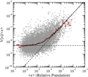
Figure 1: $\{\langle x_{i}\rangle,V[x_{i}]/\langle x_{i}\rangle\}$ pairs for each Spanish municipality. Red Triangles: median values. Solid black: fit to the median following Eq. (3). Dashed black lines: Finite-size’s fluctuations are constant, while the multiplicative regime is given by a straight line.

Let us pass now to step II), i.e., to spatial correlations. The distance between cities is $r_{ij}$ for the $i,j$-th ones. The correlation coefficient reads

$$c_{ij}=\mathrm{Cor}[\dot{x}_{i},\dot{x}_{j}]=\frac{\mathrm{Cov}[\dot{x}_{i},\dot{x}_{j}]}{\sqrt{V[\dot{x}_{i}]V[\dot{x}_{j}]}},$$ (4)

where we use the covariance $\mathrm{Cov}[\dot{x}_{i},\dot{x}_{j}]=\langle[\dot{x}_{i}-\langle\dot{x}_{i}\rangle][\dot{x}_{j}-\langle\dot{x}_{j}\rangle]\rangle$. Fig. 2 displays the empirical distribution $p(r,c)$ of the pairs $\{r_{ij},c_{ij}\}$ for Spanish cities of population $>20000$ inhabitants ($x>4\times 10^{-4}$, $n=396$), where proportional growth clearly dominates over finite-size noise (see Fig. 1). We base bottom panel of Fig. 2 on an histogram of the distance-correlation pairs, normalized along the $c$ direction (using intervals of $\Delta\ln(r)=0.1$ and $\Delta c=1/15$) in a window such that $1.7<\ln(r_{ij})<6$. We have applied a “moving average” of 10 points in the $\ln(r)$ direction so as to get a smoother surface for guiding the eye. A clear dependence on the distance becomes evident. The ensuing distribution perfectly adjusts the expected correlation coefficient’s distribution for a bivariate normal distribution given in Ref. pc, . Using a finite number of data-points $T$, we name this distribution as $P(c,C,T)$ where $c$ stands for the correlation-value that one might numerically obtains using Eq. (4), and $C$ for the actual correlation value. We assume for the latter the analytical form

$$C(r)=\frac{C(0)}{1+|r/r_{0}|^{\alpha}},$$ (5)

where $C(0)$, $r_{0}$, and $\alpha$ are adjustable parameters. $P(c,C,T)$ and $p(r,c)$ become then related via $p(r,c)=P[c,C(r),T]$ (see Fig. 2). We have found that the empirical median value of the correlation, measured in the same intervals $\Delta\ln(r)$ for a window $5<r_{ij}<1000$ km, nicely fits the above expression with $C(0)=0.254\pm 0.009$, $r_{0}=74\pm 6$ km, $\alpha=2.1\pm 0.3$, and a goodness coefficient of $R^{2}=0.996$ (Fig. 2). Remarkably enough, for large distances one has $C(r)\sim 1/r^{2}$, in agreement with the Gravity Modelgmodel . For the smallest cities ($x<2\times 10^{-5}$) no evidence of spatial correlation is encountered because of numerical noise $\propto\sqrt{x}$, confirming our expectations. For mid-populated cities we find a mixture between the two regimes.

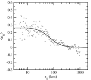
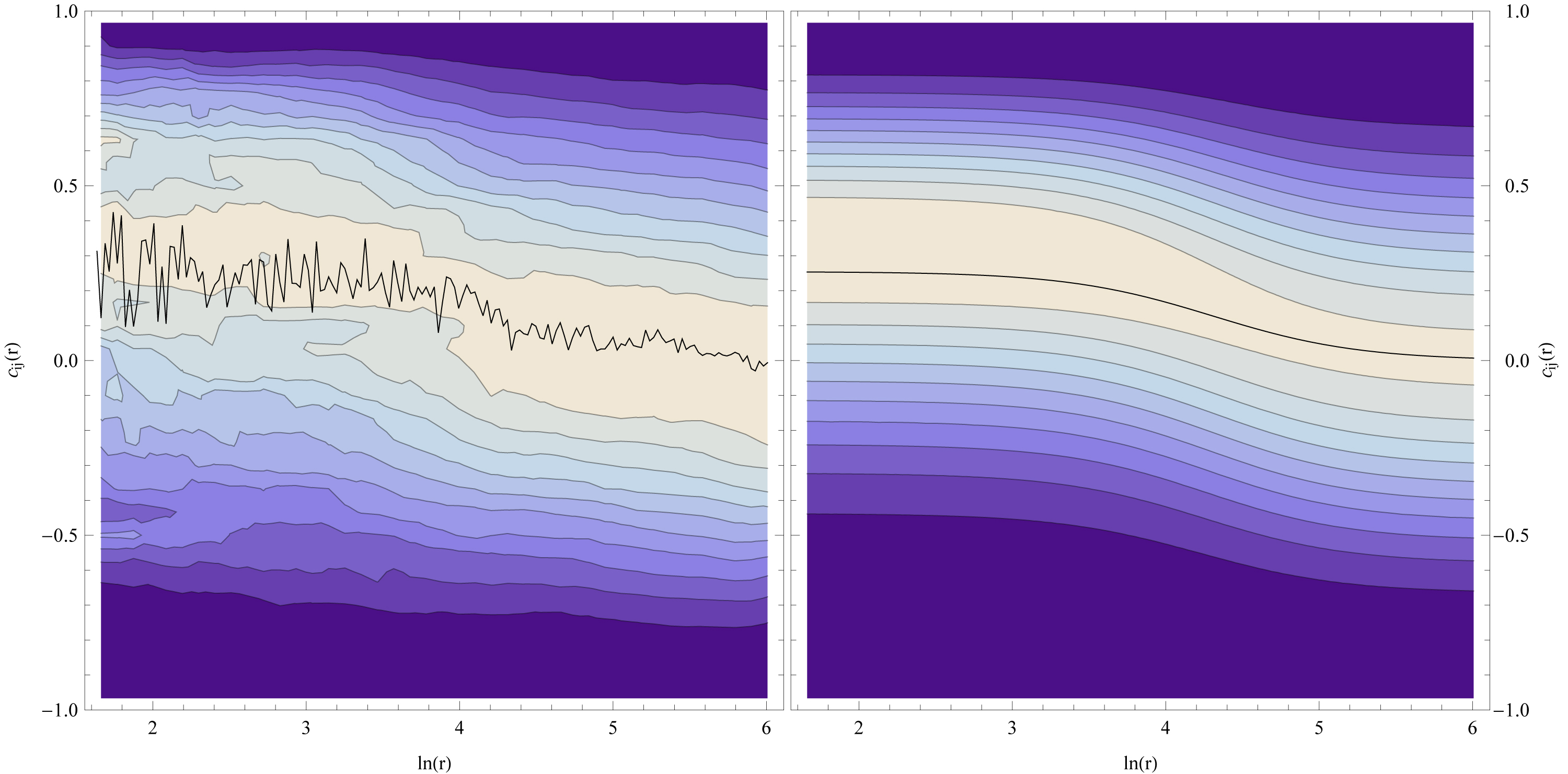
Figure 2: Top panel: Empirical mean correlation vs. distance (points), fitted to Eq. (5) (line). Bottom panels: empirical $p(r,c)$ and theoretical $P[c,C(r),T]$ distributions, together with the pertinent mean value (black line).

We pass now to step III), time-correlations. Consider i) the $n$-cities-average and variance such that

$$\langle\dot{x}(t)\rangle=\frac{1}{n}\sum_{i=1}^{n}\dot{x}_{i}(t),\leavevmode\nobreak\ V[\dot{x}(t)]=\frac{1}{n}\sum_{i=1}^{n}[\dot{x}_{i}(t)-\langle\dot{x}(t)\rangle]^{2},$$ (6)

and ii) the ensuing correlation coefficient. We estimate time-correlations via the average

$$c(\Delta t)=\frac{1}{T-\Delta t}\sum_{t=1}^{T-\Delta t}\mathrm{Cor}[\dot{x}(t),\dot{x}(t+\Delta t)].$$ (7)

Here $\Delta t$ adopts the discrete values 1, 2, 3,$\ldots$, T-1. Fig. 3 depicts results for the major Spanish cities, as in the previous case. The ensuing temporal dependence can be parameterized using the expression $c(\Delta t)=ae^{-\gamma\Delta t}$. We find $1/\gamma=17.2\pm 1.3$ years and $a=0.70\pm 0.02$, with a goodness coefficient $R^{2}=0.997$. Again, correlations are not clearly discernible in the case of small-population cities, telling us that a finite-size noise, proportional to $\sqrt{x}$, is indeed independent of time. The transition between both regimes is depicted in Fig. 3. We display the empirical value of $c(\Delta t=1)$ as a function of the population in intervals of $\Delta\ln(x)=0.25$. Growth from $0$ to $\sim 0.7$ is clearly visible.

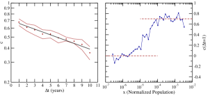
Figure 3: Left: Empirical correlation vs. time (dots) fitted to an exponential function (straight line). The red lines represent the standard deviation of the sum of Eq. (6). Note the log-scale on the vertical axis. Right: One-year correlation vs. relative population, where the transition from uncorrelated finite-size noise regime (zero correlation) to correlated proportional growth regime ($C(1)\sim 0.7$) is clearly appreciated.

In our final (IV) step, we advance a dynamical model able to reproduce the three empirical results we have encountered above, namely, i) uncorrelated numerical noise, independent from $r,t$, for small cities together with proportional growth for large populations, ii) Lorentz-type spatial correlations, and iii) exponential time-correlation. We propose here the Langevin-like equation langevin

$$\dot{x}_{i}(t) = x_{i}(t)v_{i}(t)+\sqrt{x_{i}(t)}w_{i}(t)$$ (8)

$$\dot{w}_{i}(t) = W_{i}(t)$$ (9)

$$\dot{v}_{i}(t) = F_{i}(t)-\gamma_{i}v_{i}(t)$$ (10)

$$F_{i}(t) = \sum_{i^{\prime}}R_{ii^{\prime}}f_{i^{\prime}}(t),$$ (11)

where i) $W_{i}(t)$ characterizes a Wiener-process ($\langle w_{i}(t)w_{j}(t+\Delta t)\rangle=V[w]\delta_{ij}\delta(\Delta t)$, where $V[w]$ is the corresponding variance), ii) $\gamma_{i}$ are dumping-parameters to be empirically determined, with regards to time-correlations, iii) the $R_{ii^{\prime}}$ are matrix-elements related to spatial correlations, and iv) $f_{i^{\prime}}(t)$ are stochastic forces. We assume that the forces fluctuate and are independent of each other, being of the form

$$\mathrm{Cov}[f_{i}(t),f_{j}(t+\Delta t)]=V_{f}\delta_{ij}\delta(\Delta t),$$ (12)

where $V_{f}$ stands for the variance of $f$. For the total force $F$ the covariance $\mathrm{Cov}[F_{i}(t),F_{j}(t+\Delta t)]\equiv K$ is

$$K=V_{f}\sum_{i^{\prime}}R_{ii^{\prime}}R_{ji^{\prime}}\delta(\Delta t)=V_{f}Q_{ij}\delta(\Delta t).$$ (13)

The matrix $Q=R\cdot R^{T}$ is normalized in such a fashion that its diagonal elements are all equal to unity, and thus $\mathrm{cor}[F_{i}(t),F_{j}(t)]=Q_{ij}$. Since $w_{i}(t)$ and $f_{i}(t)$ are not correlated by definition, Eq. (3) in automatically fulfilled from the variance of $\dot{x}_{i}(t)$ with $\sigma^{2}=V[v_{i}]$ and $\sigma_{1/2}^{2}=V[w]$. If the $w-$term is the dominant one (low population) there is no correlation among cities (nor in time) since we deal with a Wiener process (no memory, either). For large populations the $v-$term dominates and we have $C_{ij}(\Delta t)=\mathrm{Cor}[\dot{x}_{i}(t),\dot{x}_{j}(t+\Delta t)]=\mathrm{Cor}[v_{i}(t),v_{j}(t+\Delta t)]$ with a general solution to the Langevin equation for $v$

$$v_{i}(t)=e^{-\gamma_{i}t}v_{i}(0)+\int_{0}^{t}d\tau e^{-\gamma_{i}(t-\tau)}F_{i}(\tau).$$ (14)

Since the initial time is arbitrary, we assume $t\rightarrow\infty$ so as to obtain the $v-$correlation

$$C_{ij}(\Delta t)=\mathrm{cor}[v_{i}(t),v_{j}(t+\Delta t)]=Q_{ij}e^{-\gamma_{j}\Delta t}\frac{2\sqrt{\gamma_{i}\gamma_{j}}}{\gamma_{i}+\gamma_{j}}.$$ (15)

Note that $2\sqrt{\gamma_{i}\gamma_{j}}/(\gamma_{i}+\gamma_{j})\in[0,1]$, and its mean value depends on the distribution of the $\gamma-$values.

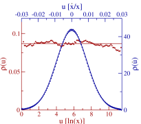
Figure 4: Equilibrium density distribution of the log-population and the relative growth obtained in the simulation (dots), compared with the thermodynamical prediction Eq. (20) (lines).

Our goal would now be nicely achieved if we could show that $Q_{ij}=1/(1+|r_{ij}/r_{0}|^{2})$. To attain such result, let us start with a result of Ref. gmodel, . The number of phone-calls between two cities can be fitted to our Lorentzian shape. If we assume such a pattern for the information flow in a human social network, we may regard the forces $F$ as resulting from the average of the stochastic forces $f$ weighted by that Lorentzian function. Thus, $F$ becomes a “coarse-grained" force. This is reflected by the definition

$$R_{ij}=\frac{2[2/\pi r_{0}^{2}]^{1/4}}{1+4|r_{ij}/r_{0}|^{2}}.$$ (16)

Let us consider for our derivation of $Q$ the continuous limit $x_{i}\rightarrow x(\mathbf{r})$, with $\mathbf{r}$ a planar spatial coordinate. $x(\mathbf{r})$ represents the relative population at $\mathbf{r}$, and the total normalized population becomes $1=\int_{S}d\mathbf{r}x(\mathbf{r}),$ where $S$ is the pertinent region’s area. Since we deal now with the coordinates $\mathbf{r}$ and $\mathbf{r}^{\prime}$ instead of the indexes $i,j$, the $R$ matrix-elements are a function $R(|\mathbf{r}-\mathbf{r}^{\prime}|)$ and the total coarse-grained force follows the convolution ($\otimes$)

$$F(\mathbf{r},t)=R(\mathbf{r})\otimes f(\mathbf{r},t)=\int_{S}d\mathbf{r}^{\prime}\frac{2[2/\pi r_{0}^{2}]^{1/4}f(\mathbf{r}^{\prime},t)}{1+4|(\mathbf{r}-\mathbf{r}^{\prime})/r_{0}|^{2}}.$$ (17)

Since the convolution of two Lorentzians of equal scale is also a Lorentzian with twice that scale-parameter, we find for the forces-correlation

$$\begin{array}[]{r}\displaystyle\mathrm{cor}[F(\mathbf{r}),F(\mathbf{r}^{\prime})]=R(|\mathbf{r}-\mathbf{r}^{\prime}|)\otimes R(|\mathbf{r}-\mathbf{r}^{\prime}|)\\ \displaystyle=Q(|\mathbf{r}-\mathbf{r}^{\prime}|)=\frac{1}{1+|(\mathbf{r}-\mathbf{r}^{\prime})/r_{0}|^{2}},\end{array}$$ (18)

i.e., the result we wished to reach. We can now interpret our equations in the following fashion: i) initially, some stochastic, independent forces $f_{i}$ act on the cities’ populations, ii) the information-flow within the population can be characterized via a Lorentzian distribution, so that the effective total force becomes the convolution of the $f_{i}$ with the distribution, iii) the observed correlations are thus Lorentzian, and at large distances decay as the square of the distance. Finally, setting $\gamma_{i}=1/17\leavevmode\nobreak\ \forall i$ and $r_{0}=74$ km, our model can reproduce the empirical correlations. The result $C(0)<1$ can be attributed to both i) some numerical, uncorrelated noise and ii) to the empirical distribution of the dumping parameters $\gamma_{i}$ [as can be verified by looking at Eq. (15)].

As an application we have performed a suitable simulation. We randomly select $n=100$ positions for population-centers on a square surface of side $L=250$ km (see Supplementary Figure). We took $V_{f}=10^{-5}$ years^-2, $\gamma=1/17$ years^-1, and $r_{0}=74$ km, forcing the population to evolve within the range $X_{0}<X<X_{M}$, with $X_{0}=1$ and $X_{M}=10^{4}$ people. We do not include finite-size effects $W$ for simplicity ($V[w]=0$). The computational cost of solving our Langevin equation can be reduced via a normal-mode treatment: define a change-of-basis matrix $A$ such that $R$ (and $Q$) become diagonal. This generates new variables $u^{\prime}_{i}(t)=\sum_{i^{\prime}}A_{ii^{\prime}}\log[X_{i}(t)]$ whose motion-equations become

$$\dot{u}^{\prime}_{i}(t)=v^{\prime}_{i}(t);\leavevmode\nobreak\ \leavevmode\nobreak\ \dot{v}^{\prime}_{i}(t)=\sqrt{\varepsilon_{i}}f^{\prime}_{i}(t)-\gamma v^{\prime}_{i}(t),$$ (19)

with $v^{\prime}_{i}(t)=\sum_{i^{\prime}}A_{ii^{\prime}}v_{i}(t)$, $f^{\prime}_{i}(t)=\sum_{i^{\prime}}A_{ii^{\prime}}f_{i}^{\prime}(t)$, and $\sqrt{\varepsilon_{i}}$ is the $i$-th eigenvalue of $R$ (with $\varepsilon_{i}$ that of $Q$). One easily checks that the forces $f^{\prime}$ are statistically equivalent to those indicated by $f$ [i.e., $\langle f^{\prime}_{i}(t)f^{\prime}_{j}(t+\Delta t)\rangle=V_{f}\delta_{ij}\delta(\Delta t)$], so that the simulation involves directly the random generation of $f^{\prime}$, without having to actually effect the basis-change. The variables $u^{\prime}_{i}(t)$ evolve in independent fashion, representing normal-mode evolution. The presence of $\sqrt{\varepsilon_{i}}$ accounts for different mode-equilibrations between $f^{\prime}$ and the dumping $\gamma$, which might be conceived as originating mass-factors. The Supplementary Figure displays the first four modes in such a way that the color at the Municipality $i$ represents the coefficient $A_{ii^{\prime}}$ for the eigenvector $i^{\prime}$ (we also shown the same decomposition for Catalonia (Spain), using the empirical value of $r_{0}$ found above). Our simulations use Verlet-integrationverlet with an interval $\delta t=1$. Equilibrium states are detected, compatible with the thermodynamics developed in Ref. thermoflow, . We verified that in equilibrium $\langle[v(t)]^{2}\rangle=V_{f}/2\gamma=8.5\times 10^{-5}$ and that the normalized equilibrium distribution $\rho(X,\dot{X})dXd\dot{X}$ follows the tenets applicable to for a thermal system confined in a constant volume. As a matter of fact, defining the log-population $u=\log(X)$ ($\dot{X}/X=\dot{u}$) one hasthermoflow

$$\rho(X,\dot{X})dXd\dot{X}=\rho(u,\dot{u})dud\dot{u}=\frac{\sqrt{\beta/2\pi}}{\log{X_{0}/X_{M}}}e^{-\frac{\beta\dot{u}}{2}},$$ (20)

where $\beta=2\gamma/V_{f}$, as depicted in Fig. 4.

Summing up, our model can be fine-tuned to any socio-geographical area via the dumping parameters $\gamma_{i}$ and the inclusion, in the forces, of any empirically-known factor that may affect population growth. There is also room to include in the correlation matrix $Q$ any other empirically-known distance-independent correlation. The model may improve on the predictive mathematical tools available today tools . Also, the study of the past evolution of the population in terms of normal models ould lead to a deeper understanding of collective human behavior at the macro-scale.

Supplementary Figure. Top: Components of the first four eigenvectos of the simulated system (from white to red: positive values; from white to blue: negative values). The surface of each municipality is defined by its Voronoi area (http://en.wikipedia.org/wiki/Voronoi_diagram). Bottom: Components of the first four eigenvectos for Catalonia, using the modelled spatial correlations (see text). The radii of the circles are proportional to the log-population.

References

- (1) J. Kemeny and J. L. Snell, Mathematical Models in the Social Sciences (MIT Press, Cambridge, Mass. 1978).
- (2) M. Schroeder, Fractals, chaos and power laws (Freeman, NY, 1990).
- (3) L. C. Malacarne, R. S. Mendes, and E. K. Lenzi, Phys. Rev. E 65, 017106 (2001).
- (4) M. Marsili, Y. C. Zhang, Phys. Rev. Lett. 80, 2741 (1998).
- (5) A. Hernando, A. Plastino. “The thermodynamics of urban population flows”. Preprint submitted to PRE (arXiv:1206.7020) (2012).
- (6) A. Hernando, A. Plastino. “The workings of the Maximum Entropy Principle in collective human behavior”. Preprint submitted to Journal of the Royal Society Interface (arXiv:1201.0905) (2012).
- (7) G. Krings et al., J. Stat. Mech. L07003 (2009).
- (8) M.C. González et al., Nature, 453, 779 (2008)
- (9) F. Simini et al. Nature, 484, 96 (2012).
- (10) Willekens, F.J. y Drewe, P. (1984) “A multiregional model for regional demographic projection”, in Heide, H. y Willekens, F.J. (ed) Demographic Research and Spatial Policy, Academic Press, Londres.
- (11) National Statistics Institute of Spain, Government of Spain (web).
- (12) Pearson product-moment correlation coefficient, from Wikipedia (web).
- (13) W.T. Coffey, Y.P. Kalmylov, J.T. Waldron, The Langevin equation, with applications to stochastic problems in Physics, Chemistry and Electrical Engineering (Second Edition), World Scientific Series in Contemporary Chemical Physics, Vol. 14.
- (14) E. W. Weisstein, MathWorld – A Wolfram Web Resource.
- (15) L. Verlet, Phys. Rev. 159, 98 (1967).