Characterisation of candidate members of (136108) Haumea’s family

Abstract

Context. From a dynamical analysis of the orbital elements of transneptunian objects (TNOs), Ragozzine & Brown reported a list of candidate members of the first collisional family found among this population, associated with (136 108) Haumea (a.k.a. 2003 EL₆₁).

Aims. We aim to distinguish the true members of the Haumea collisional family from interlopers. We search for water ice on their surfaces, which is a common characteristic of the known family members. The properties of the confirmed family are used to constrain the formation mechanism of Haumea, its satellites, and its family.

Methods. Optical and near-infrared photometry is used to identify water ice. We use in particular the $CH_{4}$ filter of the Hawk-I instrument at the European Southern Observatory Very Large Telescope as a short $H$-band ($H_{S}$), the $(J-H_{S})$ colour being a sensitive measure of the water ice absorption band at 1.6 $\mu m$.

Results. Continuing our previous study headed by Snodgrass, we report colours for 8 candidate family members, including near-infrared colours for 5. We confirm one object as a genuine member of the collisional family (2003 UZ₁₁₇), and reject 5 others. The lack of infrared data for the two remaining objects prevent any conclusion from being drawn. The total number of rejected members is therefore 17. The 11 confirmed members represent only a third of the 36 candidates.

Conclusions. The origin of Haumea’s family is likely to be related to an impact event. However, a scenario explaining all the peculiarities of Haumea itself and its family remains elusive.

1 Introduction

The dwarf planet (136 108) Haumea (Santos-Sanz et al. 2005) is among the largest objects found in the Kuiper Belt (Rabinowitz et al. 2006, Stansberry et al. 2008), together with Pluto, Eris, and Makemake. It is a highly unusual body with the following characteristics:

1. It has a very elongated cigar-like shape (Rabinowitz et al. 2006, Lellouch et al. 2010).

2. It is a fast rotator ($P_{rot}\sim 3.9$ h, Rabinowitz et al. 2006).

3. It has two non-coplanar satellites (Brown et al. 2006, Ragozzine & Brown 2009, Dumas et al. 2011).

4. It is the largest member of a dynamical family (Brown et al. 2007, Ragozzine & Brown 2007), whose velocity dispersion is surprisingly small (Schlichting & Sari 2009, Leinhardt et al. 2010).

5. Its surface composition is dominated by water ice (Tegler et al. 2007, Trujillo et al. 2007, Merlin et al. 2007, Pinilla-Alonso et al. 2009, Dumas et al. 2011), yet it has a high density of 2.5-3.3 g cm^-3 (Rabinowitz et al. 2006).

6. It surface has a hemispherical colour heterogeneity, with a dark red “spot” on one side (Lacerda et al. 2008, Lacerda 2009).

Brown et al. (2007) proposed that Haumea suffered a giant collision that ejected a large fraction of its ice mantle, which formed both the two satellites and the dynamical family and left Haumea with rapid rotation. A number of theoretical studies have since looked at the family formation in more detail (see Sect. 5).
A characterisation of the candidate members (35 bodies listed by Ragozzine & Brown 2007, including Haumea itself) however showed that only 10 bodies out of 24 studied share their surface properties with Haumea (Snodgrass et al. 2010), and can thus be considered genuine family members. Moreover, these confirmed family members cluster in the orbital elements space (see Fig. 4 in Snodgrass et al. 2010), and the highest velocity found was $\sim$123 m s^-1 (for 1995 SM₅₅).
We report on follow-up observations to Snodgrass et al. (2010) of 8 additional candidate members of Haumea’s family. We describe our observations in Sect. 2, the colour measurements in Sect. 3, the lightcurve analysis and density estimates in Sect. 4, and we discuss in Sect. 5 the family memberships of the candidates and the implication of these for the characteristics of the family.

2 Observations and data reduction

We performed our observations at the European Southern Observatory (ESO) La Silla and Paranal Very Large Telescope (VLT) sites (programme ID: 84.C-0594). Observations in the visible wavelengths ($BVRi$ filters) were performed using the EFOSC2 instrument (Buzzoni et al. 1984) mounted on the NTT (since April 2008; Snodgrass et al. 2008); while near-infrared observations ($J$, $CH_{4}$ filters) were performed using the wide-field camera Hawk-I (Pirard et al. 2004, Casali et al. 2006, Kissler-Patig et al. 2008) installed on the UT4/Yepun telescope. We use the medium-width $CH_{4}$ filter as a narrow H band (1.52–1.63 $\mu$m, hereafter $H_{S}$) to measure the $J$-$H_{S}$ colour as a sensitive test for water ice (see Snodgrass et al. 2010, for details). We list the observational circumstances in Table 1.
We reduced the data in the usual manner (i.e., bias subtraction, flat fielding, sky subtraction, as appropriate). We refer readers to Snodgrass et al. (2010) for a complete description of the instruments and the methods we used to detect the targets, and both measure and calibrate their photometry.
For each frame, we used the SkyBoT cone-search method (Berthier et al. 2006) to retrieve all known solar system objects located in the field of view. We found 3 main-belt asteroids, and the potentialy hazardeous asteroid (29 075) 1950 DA (e.g. Giorgini et al. 2002, Ward & Asphaug 2003), in our frames. We report the circumstances of their serendipitous observations in Table 1 and their apparent magnitude in Table 2, together with the family candidates and our back-up targets.

Table 1: Observational circumstances.

Object		$\Delta^{\mathrm{a}}$	$r^{\mathrm{b}}$	$\alpha^{\mathrm{c}}$	Runsd
(#)	(Designation)	(AU)	(AU)	(°)
	1999 CD 158	47.5	46.5	0.5	B
	1999 OK 4	46.5	45.5	0.3	$\star$
	2000 CG 105	45.8	46.8	0.1	A,B
	2001 FU 172	32.2	32.0	1.7	A
	2002 GH 32	43.2	42.9	1.2	B
	2003 HA 57	32.7	32.3	1.6	A
	2003 UZ 117	39.4	39.4	1.4	A
	2004 FU 142	33.5	33.2	0.0	A
	2005 CB 79	39.9	39.0	0.4	A
	2005 GE 187	30.3	30.2	1.9	A
24	Themis	3.4	4.0	12.0	B
10 199	Chariklo	13.8	13.6	4.1	B
29 075	1950 DA	0.8	1.0	62.7	A
158 589	Snodgrass	3.5	3.1	15.5	A
104 227	2000 EH 125	3.0	2.5	18.5	A
202 095	2004 TQ 20	2.2	1.9	2.4	A
	2010 CU 19	1.3	1.6	0.6	A

3 Colours

We report the photometry of all the objects in Table 2, where we give the apparent magnitude in each band, averaged over all the observations. We used a common sequence of filters (RBViR) to observe all the objects. This limits the influence of the shape-related lightcurve on the colour determination. In Table 3, we report the average colours of all the family candidates observed here, and refer to Snodgrass et al. (2010) for a complete review of the published photometry.

Table 2: Mean apparent magnitudes for each object.

Object	$B$	$V$	$R$	$i$	$J$	$CH_{4}$
1999 CD 158	–	–	–	–	20.79 $\pm$ 0.08	20.44 $\pm$ 0.10
1999 OK 4	24.90 $\pm$ 0.16	24.54 $\pm$ 0.17	23.95 $\pm$ 0.14	23.64 $\pm$ 0.20	–	–
2000 CG 105	24.32 $\pm$ 0.14	23.62 $\pm$ 0.10	23.15 $\pm$ 0.05	22.61 $\pm$ 0.07	21.89 $\pm$ 0.10	21.64 $\pm$ 0.14
2001 FU 172	23.40 $\pm$ 0.05	21.73 $\pm$ 0.04	20.82 $\pm$ 0.03	19.99 $\pm$ 0.03	–	–
2002 GH 32	–	–	–	–	21.49 $\pm$ 0.12	21.31 $\pm$ 0.15
2003 HA 57	24.37 $\pm$ 0.09	23.48 $\pm$ 0.09	22.96 $\pm$ 0.05	22.69 $\pm$ 0.12	–	–
2003 UZ 117†	21.86 $\pm$ 0.09	21.34 $\pm$ 0.08	21.09 $\pm$ 0.08	20.67 $\pm$ 0.07	–	–
2003 UZ 117⋆	22.04 $\pm$ 0.10	21.32 $\pm$ 0.06	21.01 $\pm$ 0.06	20.62 $\pm$ 0.06	–	–
2005 CB 79	–	–	20.29 $\pm$ 0.01	–	–	–
2005 GE 187	23.73 $\pm$ 0.14	22.91 $\pm$ 0.12	22.23 $\pm$ 0.09	21.49 $\pm$ 0.06	–	–
1950 DA	19.59 $\pm$ 0.07	19.15 $\pm$ 0.06	18.82 $\pm$ 0.02	18.56 $\pm$ 0.04	–	–
2000 EH 125	21.58 $\pm$ 0.03	20.78 $\pm$ 0.02	20.37 $\pm$ 0.02	20.05 $\pm$ 0.03	–	–
2004 TQ 20	21.93 $\pm$ 0.06	21.23 $\pm$ 0.07	21.19 $\pm$ 0.08	20.73 $\pm$ 0.07	–	–
2010 CU 19	–	19.26 $\pm$ 0.04	–	–	–	–
Chariklo	–	–	–	–	16.98 $\pm$ 0.02	16.86 $\pm$ 0.02
Themis	–	–	–	–	12.38 $\pm$ 0.02	12.25 $\pm$ 0.02
Snodgrass	22.40 $\pm$ 0.14	21.61 $\pm$ 0.10	21.20 $\pm$ 0.05	20.69 $\pm$ 0.08	–	–

From these average colours, we calculate reflectances by comparing them to the solar colours. We also report the visible slope for each object (%/100 nm) in Table 3, calculated from the reflectances via a linear regression over the full $BVRi$ range. The reflectance “spectra” of the candidates from this photometry are shown in Fig. 1. The reflectance spectrum of (136 108) Haumea from Pinilla-Alonso et al. (2009) is shown for comparison to the photometry. For all the objects but 1999 CD₁₅₈ (Delsanti et al. 2004), the link between the visible and near-infrared wavelengths was made by extrapolating the visible spectral slope to the $J$-band, owing to a lack of simultaneous observations. Among these objects, 2002 GH₃₂ has a distinctive spectral behaviour. It displays a slight dip at 1.5 $\mu$m despite a red slope, as its $(J-H_{S})$ colour (0.18 $\pm$ 0.19) is slightly bluer than that of the Sun (0.28; Snodgrass et al. 2010). Given the uncertainty in this point, and the red optical slope, we do not believe that this is evidence of strong water ice absorption.
From the visible and near-infrared colours that we report here, we confirm that 2003 UZ₁₁₇ is a genuine family member, in agreement with Ragozzine & Brown (2007) and Snodgrass et al. (2010), and reject 1999 CD₁₅₈, 2000 CG₁₀₅, 2001 FU₁₇₂, 2002 GH₃₂, and 2005 GE₁₈₇. The TNO 1999 OK₄ remains a possible candidate, as it has a neutral slope in the visible, but the poor signal-to-noise ratio of the data for this faint target does not allow us to draw a stronger conclusion. In any case, a neutral slope by itself does not confirm family membership without near-infrared observations. This object is dynamically very near to the centre of the family and remains worthy of further investigation. 2003 HA₅₇ has a red slope, but not a very strong one. It is further from the centre of the distribution, with $\delta v>200$ m s^-1, so it is unlikely to be a family member (see below). We cannot firmly conclude anything about the membership of 1999 OK₄ and 2003 HA₅₇. The current number of confirmed family members is 11 over 36 (including Haumea and an additional dynamical candidate (2009 YE₇) that was found and directly confirmed by Trujillo et al. (2011)), or 31%. The number of rejected candidates is 17 over 36, hence 47% of the population, and there are only 8 objects whose status remains unknown.

Figure 1: Visible and near-infrared photometry for the candidate family members (see Table 3). The data are normalized at 0.55 $\mu$m ($V$ filter). The spectrum of Haumea (taken from Pinilla-Alonso et al. 2009) is shown for comparison in each.

Table 3: Average colours in $BVRiJH_{S}$, and assessment of likely membership based on these colours.

Object	$(B-V)$	$(V-R)$	$(R-i)$	$(R-J$)	$(J-H_{S})^{\star}$	Vis. slope	Ref.	Family?
Designation	(mag.)	(mag.)	(mag.)	(mag.)	(mag.)	(%/100nm)
1999 CD 158	0.83 $\pm$ 0.06	0.51 $\pm$ 0.05	0.54 $\pm$ 0.06	1.38 $\pm$ 0.09	0.35 $\pm$ 0.12	15.8 $\pm$ 0.6	1,5,8	N
1999 OK 4	0.36 $\pm$ 0.23	0.58 $\pm$ 0.22	0.32 $\pm$ 0.24	–	–	1.4 $\pm$ 18.1	8	?
2000 CG 105	0.71 $\pm$ 0.17	0.56 $\pm$ 0.11	0.77 $\pm$ 0.29	–	0.25 $\pm$ 0.17	11.3 $\pm$ 4.3	5,8	N
2000 JG 81	–	0.50 $\pm$ 0.11	0.33 $\pm$ 0.12	–	–	5.6 $\pm$ 21.6	6	?
2001 FU 172	1.67 $\pm$ 0.06	0.91 $\pm$ 0.05	0.83 $\pm$ 0.03	–	–	64.2 $\pm$ 4.3	5,8	N
2002 GH 32	0.91 $\pm$ 0.06	0.66 $\pm$ 0.06	0.56 $\pm$ 0.05	–	0.18 $\pm$ 0.19	24.8 $\pm$ 4.7	5,8	N
2003 HA 57	0.89 $\pm$ 0.13	0.52 $\pm$ 0.10	0.27 $\pm$ 0.12	–	–	8.7 $\pm$ 11.6	8	?
2003 UZ 117	0.52 $\pm$ 0.12	0.25 $\pm$ 0.11	0.42 $\pm$ 0.11	–	-0.74 $\pm$ 0.16	-0.5 $\pm$ 3.7	2-5,7,8	Y
2005 GE 187	0.81 $\pm$ 0.18	0.69 $\pm$ 0.14	0.74 $\pm$ 0.11	1.22 $\pm$ 0.19	0.65 $\pm$ 0.14	32.8 $\pm$ 12.3	5,8	N
Haumea	0.64 $\pm$ 0.01	0.33 $\pm$ 0.01	0.34 $\pm$ 0.01	0.88 $\pm$ 0.01	-0.60 $\pm$ 0.11	-0.6 $\pm$ 0.9	5	Y

[1] Delsanti et al. (2004); [2] DeMeo et al. (2009); [3] Pinilla-Alonso et al. (2007); [4] Alvarez-Candal et al. (2008); [5] Snodgrass et al. (2010, and references therein); [6] Benecchi et al. (2011); [7] Trujillo et al. (2011); [8] This work. Where colours for a given object are published by multiple authors, we quote a weighted mean.

4 Rotation and density

To constrain the density of family members, and therefore test the hypothesis that they are formed of almost pure water ice, we investigated their rotational lightcurves. In the February 2010 observing run, we performed a time series of $R$-band photometry on 2005 CB₇₉, which was demonstrated to be a family member by Schaller & Brown (2008) and Snodgrass et al. (2010). We measured 69 points over the course of three nights, with a typical uncertainty in each measurement of 0.03 magnitudes. We observed a variation of around 0.15 magnitudes, but found no convincing periodicity. Thirouin et al. (2010) found a period of 6.76 hours and a similar magnitude range.
A total of 8 family members have published lightcurve measurements (Table 4). These can be used to estimate the density by two methods. By either balancing gravitational and centrifugal forces for an assumed strengthless (rubble pile) body, as applied to asteroids (Pravec et al. 2002) and comets (Snodgrass et al. 2006), or by assuming a fluid equilibrium shape (i.e., a Jacobi ellipsoid), which may be more appropriate for large icy bodies such as TNOs (Lacerda & Jewitt 2007). The densities of TNOs derived from lightcurves was reviewed by Duffard et al. (2009) and Thirouin et al. (2010). Of particular interest is the high value of 2.38 g cm^-3 determined for 2003 OP₃₂, which is a large confirmed family member with a strong water-ice spectrum (Brown et al. 2007). The quoted value is considerably higher than that of water ice, and close to the value determined for Haumea itself (2.61 g cm^-3, Thirouin et al. 2010), and is therefore inconsistent with this body being a pure water-ice fragment from the original Haumea’s outer mantle. However, this (minimum) density is derived assuming that the best-fit single peaked period of 4.05 hours is the correct spin rate, which can only be true if the variation is due to an albedo patch on a spheroidal body, i.e., a Maclaurin spheroid rather than a Jacobi ellipsoid. If the true rotation period is instead twice this value (i.e., the double peaked lightcurve is due to shape instead of albedo features), then the required minimum density is 0.59 g cm^-3, which provides a far weaker constraint. No other family member (aside from Haumea itself) has a reported rotation rate fast enough to require a high density (Table 4 and Fig. 2).

Table 4: Rotational periods (SP: single peak, DP: double peak) of family candidates.

Object		$H$	$d^{\dagger}$	$\Delta m$	Period SP		Period DP		Ref.	$\rho_{m}^{\star}$
#	Designation		(km)		(h)		(h)			(g cm-3)
24835	1995 SM 55	4.8	174	0.19	4.04  $\pm$	0.03	8.08  $\pm$	0.03	2	0.60
19308	1996 TO 66	4.5	200	0.32	3.96  $\pm$	0.04	7.92  $\pm$	0.04	2	0.63
							11.9		5
							6.25  $\pm$	0.03	1
86047	1999 OY 3	6.74	71
55636	2002 TX 300	3.2	364	0.08	8.16				8	0.16
					8.12  $\pm$	0.08	16.24  $\pm$	0.08	3
					12.10  $\pm$	0.08	24.20  $\pm$	0.08	3
					7.89  $\pm$	0.03	15.78  $\pm$	0.03	4
136108	Haumea	0.01	1313	0.28			3.9154  $\pm$	0.0001	6,8,10	2.56
120178	2003 OP 32	3.95	258	0.13	4.05				8	0.59
	2003 SQ 317	6.3	87	1.00	3.74  $\pm$	0.10	7.48  $\pm$	0.10	9	0.5
	2003 UZ 117	5.3	138	0.20	$\sim$6				7	0.27
	2005 CB 79	4.7	182	0.04	6.76				8	0.21
145453	2005 RR 43	4.0	252	0.12	7.87				8	0.38
					5.08  $\pm$	0.03			7
	2009 YE 7	4.4	209

[1] Hainaut et al. (2000); [2] Sheppard & Jewitt (2002); [3] Sheppard & Jewitt (2003); [4] Ortiz et al. (2004); [5] Belskaya et al. (2006); [6] Lacerda et al. (2008); [7] Perna et al. (2010); [8] Thirouin et al. (2010); [9] Snodgrass et al. (2010); [10] Lellouch et al. (2010)

Instead of considering individual rotation periods, we consider the family as a whole. Fig. 2 compares all confirmed family members (black points) with all other TNO lightcurve measurements (open circles) taken from the compilation of Duffard et al. (2009). The rotation period plotted assumes a double-peaked period for all objects (i.e., shape-controlled lightcurve), and the curved lines show densities calculated based on the assumption of hydrostatic equilibrium (Jacobi ellipsoids). Rotation rates from the Duffard et al. (2009) table are taken at face value (no further attempt has been made to judge the reliability of the determined periods), with the exception of two very short rotation periods (1996 TP₆₆ and 1998 XY₉₅, with single peak periods of 1.96 and 1.31 hours respectively; Collander-Brown et al. 1999, 2001) that appear in the table despite the original authors stating that these were unrealistic (and statistically insignificant) mathematical best fits. We removed these values and regard the rotation periods of these two objects as unknown. For all other objects where there are both multiple period determinations and no preferred period in Duffard et al., we take the shortest period to give the highest possible minimum density.

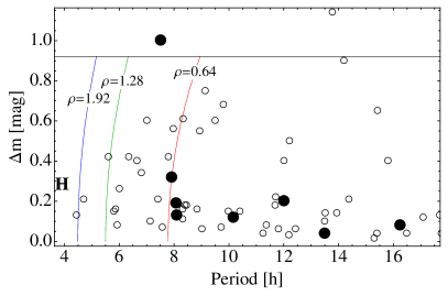
Figure 2: Lightcurve amplitude ($\Delta m$) as a function of the rotation period (in hours) for the TNOs in the vicinity of Haumea. Filled and open circles stand for confirmed family members and background population (from Duffard et al. 2009, Thirouin et al. 2010), respectively. The letter H shows the position of Haumea. Vertical blue, red, and green curves are the limit for stability, assuming the objects are in hydrostatic equilibrium, i.e., stable objects left of a line are denser than the number in the label (in g cm^-3). Objects above the black line ($\Delta m$ $\sim$ 0.9 mag) are unstable (under the hydrostatic equilibrium assumption), and are likely contact binaries.

Seven of the eight family members fall into the relatively long-period (low-density) area of this plot, with $\rho\leq 0.64$ g cm^-3. The exception is 2003 SQ₃₁₇, which has a large lightcurve amplitude (Snodgrass et al. 2010), implying that it is likely to be a contact binary (therefore the Jacobi ellipsoid model does not hold, Lacerda & Jewitt 2007).
A direct comparison between the densities of family members and other TNOs is not straightforward since analysis of the rotational properties based on hydrostatic equilibrium can in general only set lower limits on the densities of the objects. We can, however, use the observed lightcurve properties (Fig. 2) to assess the probability that the family members and other TNOs were drawn from the same 2-D distribution in spin period vs. $\Delta m$. To do so, we use the 2-D Kolmogorov-Smirnov (K-S) test (Peacock 1983). The 2-D K-S test uses the $Z$ statistic (the maximum absolute difference between the cumulative distributions of the samples) to quantify the dissimilarity between the distributions of two samples. The larger the value of $Z$, the more dissimilar the distributions.
We exclude Haumea and objects with $\Delta m$ $>$ $0.9$ mag from this calculation: Haumea is not representative of the densities of its family, and objects with very large $\Delta m$ obey a different relationship between rotational properties and bulk density (Lacerda & Jewitt 2007). Considering the two populations made of the 7 family members and the 64 background TNOs, we obtain a value of $Z=1.276$. The corresponding probability that the $P$ vs. $\Delta m$ distributions of family members and other TNOs would differ by more than they do is $P_{>Z}=0.040$. If we furthermore discard objects with $\Delta m$ $<$ $0.1$ mag that are unlikely to be Jacobi ellipsoids, the populations are made of 5 and 42 TNOs respectively, and the K-S probability lowers to $P_{>Z}=0.014$. These low values of $P_{>Z}$ suggest that the family members have different rotational properties from other TNOs, although the current data are still insufficient to quantitatively compare the densities of family members and other TNOs.
We note that the small numbers of objects and rather uncertain rotation periods for many, make such an analysis approximate at best, i.e., this is not yet a statistically robust result. Furthermore, many of the larger objects with long rotation periods and low lightcurve amplitudes are likely to be spheroidal rather than ellipsoidal bodies, with single peak lightcurves due to albedo features (Pluto is an example), and we have made no attempt to separate these from the shape controlled bodies in Fig. 2. In addition, no restriction on orbit type (e.g., classicals, scattered disk) is imposed on the objects in Fig. 2, as the total number of TNOs with lightcurves in the Duffard et al. (2009) compilation is still relatively low (67 objects included in Fig. 2).

5 Family membership and formation scenario

5.1 Orbital elements

We show in Fig. 3 the orbital parameters (semi-major axis, inclination and eccentricity) of the candidates. As already noted by Snodgrass et al. (2010), the confirmed family members cluster tightly around the centre of the distribution in both plots, at the supposed location of the pre-collision Haumea (Haumea itself having now a higher eccentricity, owing to its interaction with Neptune through orbital resonance, see Ragozzine & Brown 2007). Water ice has been detected on all the objects within the isotropic $\delta v$ limit of 150 m s^-1 defined for a collision-formation scenario by Ragozzine & Brown (2007), while only 14% of the objects with a larger velocity dispersion harbour water ice surfaces. Even assuming that all the as-yet uncharacterised candidates have water ice on their surfaces brings this number to only 32%, which significantly differs from the proportion inside the 150 m s^-1 region. The probability of randomly selecting the single most clustered set of 11 out of a sample of 36 is only $10^{-9}$. The clustering of water-bearing objects around the position of the proto-Haumea in orbital parameter space is therefore real, with a very high statistical significance. Wider photometric surveys of the trans-Neptunian region (Trujillo et al. 2011, Fraser & Brown 2012) find no further bodies with the strong water-ice spectrum characteristic of the family, which appears to be a unique cluster of objects.

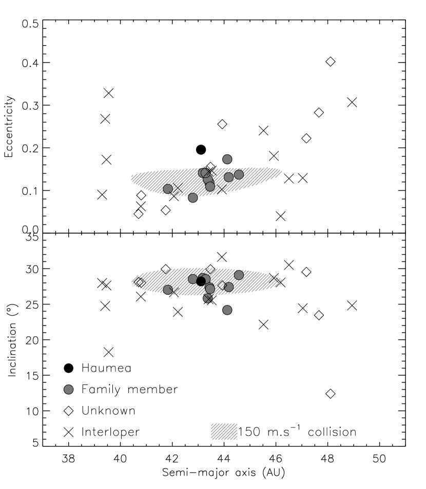
Figure 3: Confirmed family members (grey filled circles with a black outline), rejected candidates: interlopers (crosses), and those with unknown surface properties (open diamonds) plotted in terms of the orbital osculating parameters semi-major axis, inclination and eccentricity. Haumea itself is shown as a black disk. We also drawn the area corresponding to a simulation of ejected particules from a nominal collision with an isotropic $\Delta v$ of 150 m s^-1 (Ragozzine & Brown 2007).

5.2 Mass of the family

We discuss below how current observations can constraint the formation scenario of Haumea and its family. We first evaluate the mass of the family by summing over all confirmed members. We evaluate the mass $M$ of each object from its absolute magnitude $H$, from

$$M=\frac{\pi\rho}{6}\left(\frac{1329}{\sqrt{p_{V}}}\right)^{3}10^{-0.6H},$$ (1)

where $p_{V}$ is the geometric albedo (assumed to be 0.7 for family members), and $\rho$ their density (assumed to be 0.64 g cm^-3, the largest found for a family member, see Fig. 2, and consistent with the typical density of TNOs, see Carry 2012). The 11 confirmed family members account for only 1% of the mass of Haumea (4 $\times$ $10^{21}$ kg, Ragozzine & Brown 2009), raising to 1.4% when also considering Hi‘iaka and Namaka, the two satellites of Haumea, as family members. Including all the 8 remaining candidates adds only another 0.01%.
This mass fraction is however a lower limit, as more icy family members can be expected to be found. The area encompassed by the confirmed family member in orbital element space (Fig. 3) is wide (6 AU). Given the small fraction of known TNOs (a couple of percent, for TNOs of 100 km diameter, see Trujillo 2008), many more objects are still to be discovered in the vicinity of Haumea. To estimate how much mass has yet to be discovered, we compare the observed cumulative size-distribution of family members with three simple models, described by power laws of the form $N(>r)\propto r^{-q}$ (Fig. 4). The observed distribution includes the satellites of Haumea (namely Hi‘aka and Namaka) which have 0.29 and 0.14 times Haumea’s diameter of 1250 km (Fraser & Brown 2009, Ragozzine & Brown 2009, Carry 2012), and is based on the observed distribution of absolute magnitudes $H$ and an assumed Haumea-like albedo of 0.7 (Table 4), with the exception of 2002 TX₃₀₀, which has a diameter determined by stellar occultation (Elliot et al. 2010). We also include the remaining candidates (open circles) that have not yet been ruled out, which are nearly all smaller (fainter) than the confirmed family members. The first model is based on the classical distribution for collisional fragments, with $q=2.5$ (Dohnanyi 1969). The second takes the size distribution for large TNOs measured by Fraser & Kavelaars (2009), $q=3.8$. The third is a simplification of the model presented by Leinhardt et al. (2010), with the mass distribution shown in their Fig. 3 approximated by a $q_{\rm M}=1.5$ power law, which corresponds to a very steep size distribution of $q=4.5$. We normalise the distribution to the largest object, Hi‘iaka, on the assumption that there are no more family members with $H\approx 3$ ($D\approx 400$ km) to be found.

Figure 4: Cumulative size distribution for confirmed (filled blue circles) and remaining candidate (open green circles) family members, compared with three power law models (see text). The models have $q=2.5$ (solid line), $q=3.8$ (dashed line) and $q=4.5$, approximating the model of Leinhardt et al. (2010), (dotted line). The satellites of Haumea, Hi‘iaka and Namaka, are represented by blue squares.

The $q=2.5$ model predicts that the largest object still to be discovered has a diameter of around 140 km, or $H\approx 5$. This corresponds to an apparent magnitude at opposition fainter than 21, which is below the detection limits of wide area TNO surveys to date (Trujillo & Brown 2003). Extrapolating this model to small sizes predicts a total mass of the family of $\sim$2% of Haumea’s mass, with nearly all of that mass in the already discovered large fragments. Models 2 and 3 predict the largest family members still to be discovered of diameters $\sim$220 km and 250 km respectively, objects at least a magnitude brighter, which would have had a chance of being found by existing surveys, depending on where in their orbits they currently are. These models cannot be extrapolated (model 2 is based on the observed TNO size distribution, which has a different slope at smaller sizes, and model 3 is a coarse approximation to the simulations by Leinhardt et al. (2010), which give a total family mass of $\sim$7% of Haumea), but they do allow there to be considerable missing mass in these large undetected bodies. These models show that in the case of a collisional size distribution we already know of all the large bodies, and all the significant mass, while steeper distributions can be observationally tested as they imply missing members with large diameters that should easily be found by new surveys (e.g., Pan-STARRS, LSST).

5.3 Family formation models

The clustering of Haumea’s family, with a low $\delta v$ between fragments, may be its most peculiar property (Marcus et al. 2011), and can be used as a strong constraint on formation models. Additionally, the models must explain the spin of Haumea and the mass and velocity dispersion of its fragments, keeping in mind that some of the original mass has been lost over time (TNO region is thought to be far less populous today than it was in the early solar system, see, e.g., Morbidelli et al. 2008). None of the models below studied the long-term stability of the satellites or the fate of ejected fragment formed during the collision/fission, but Lykawka et al. (2012) found that about 25% of the fragments would not survive over 4 Gyr, the first Gyr being when most of the dynamical evolution took place.
The model by Schlichting & Sari (2009), which describes the cataclysmic disruption of a large icy satellite around Haumea, reproduces the velocity distribution of the family, and gives an original mass of the family of around 1% of Haumea. The spin period of Haumea, however, is expected to be longer than observed, based on considerations on physics of impacts and tides in the system (see arguments by Leinhardt et al. 2010, Ortiz et al. 2012, and reference therein). The rotational fission scenario presented by Ortiz et al. (2012) does reproduce Haumea’s spin period, but predicts a velocity distribution several times higher than observed. a peculiar kind of graze and merge impact can explain Haumea’s shape and spin, and a family of icy objects with low $\delta v$, that have a total original mass $\sim 7\%$ of the proto-Haumea. This mass is higher than that observed, but may be consistent with objects lost from the family by dynamical interactions.
Cook et al. (2011) suggested an alternative solution, that bodies without the unique strong water ice signature could also be family members but from different layers in a differentiated proto-Haumea. This black sheep hypothesis has fewer observational constraints, as currently too few objects are known to be able to identify the family by dynamics alone (i.e., without spectral information), so it is possible to imagine a higher mass and larger velocity dispersion. However, as discussed above, the clustering of family members with icy surfaces suggests that the true family members have a small velocity dispersion. Further modelling is required to tell whether a low $\delta v$ population of pure ice bodies can come from a population of a mixture of higher-velocity collisional fragments.

6 Conclusions

We have presented optical and near-infrared colours for 8 of the 36 candidate members of Haumea’s collisional family (Ragozzine & Brown 2009), in addition to the 22 objects we already reported (Snodgrass et al. 2010). We confirmed the presence of water ice on the surface of 2003 UZ₁₁₇, confirming its link with Haumea, and rejected 5 other candidates (following our prediction that most of the remaining objects would be interlopers, Snodgrass et al. 2010).
Of the 36 family member candidates including Haumea, only 11 (30%) have been confirmed on the basis of their surface properties, and a total of 17 have been rejected (47%). All the confirmed members are tightly clustered in orbital elements, the largest velocity dispersion remaining 123.3 m s^-1 (for 1995 SM₅₅). These fragments, together with the two satellites of Haumea, Hi‘iaka and Namaka, account for about 1.5% of the mass of Haumea.
The current observational constraints on the family formation can be summarised as:

1. A highly clustered group of bodies with unique spectral signatures.

2. An elongated and fast-rotating largest group member.

3. A velocity dispersion and total mass lower than expected for a catastrophic collision with a parent body of Haumea’s size, but a size distribution consistent with a collision.

Various models have been proposed to match these unusual constraints, although so far none of these match the full set of constraints.