Optimal Data Collection For Informative
Rankings Expose Well-Connected Graphs

Abstract

Given a graph where vertices represent alternatives and arcs represent pairwise comparison data, the statistical ranking problem is to find a potential function, defined on the vertices, such that the gradient of the potential function agrees with the pairwise comparisons. Our goal in this paper is to develop a method for collecting data for which the least squares estimator for the ranking problem has maximal Fisher information. Our approach, based on experimental design, is to view data collection as a bi-level optimization problem where the inner problem is the ranking problem and the outer problem is to identify data which maximizes the informativeness of the ranking. Under certain assumptions, the data collection problem decouples, reducing to a problem of finding multigraphs with large algebraic connectivity. This reduction of the data collection problem to graph-theoretic questions is one of the primary contributions of this work. As an application, we study the Yahoo! Movie user rating dataset and demonstrate that the addition of a small number of well-chosen pairwise comparisons can significantly increase the Fisher informativeness of the ranking. As another application, we study the 2011-12 NCAA football schedule and propose schedules with the same number of games which are significantly more informative. Using spectral clustering methods to identify highly-connected communities within the division, we argue that the NCAA could improve its notoriously poor rankings by simply scheduling more out-of-conference games.

Keywords: Ranking, active learning, scheduling, optimal experimental design, graph synthesis, algebraic connectivity

1 Introduction

The problem of statistical ranking arises in a variety of applications, where a collection of alternatives is ranked based on pairwise comparisons. Methods for ranking must address a number of inherent difficulties including incomplete, inconsistent, and imbalanced data. Despite and possibly as a consequence of these difficulties, although ranking from pairwise comparison data is an old problem (David, 1963), there have been several recent contributions to the subject with applications in social networking, game theory, e-commerce, and logistics (Langville and Meyer, 2012; Osting et al., 2013b; Hirani et al., 2011; Jiang et al., 2010; Callaghan et al., 2007).

The statistical ranking problem can be generally posed as finding an estimate for a ranking, $\phi$, for a set of alternatives from a dataset which consists of (i) a set of alternative pairs which have been queried, $w$, and (ii) noisy, cardinal pairwise comparisons for those alternative pairs, $y$. We symbolically express an estimator for the ranking problem,

$$\hat{\phi}_{w}=\mathcal{R}(y,w),$$ (1)

where the dependence of the ranking, $\hat{\phi}_{w}$, on the queried pairs (data collected), $w$, is emphasized by the subscript.

Consider the dependence of a ranking, $\hat{\phi}_{w}$, satisfying (1), on the collected data, $w$. Generally speaking, for a fixed number of alternatives, the more alternative pairs which have been queried, the more informative we expect the ranking, $\hat{\phi}_{w}$. That is, there is a tradeoff between the amount of pairwise data collected and the informativeness of the ranking. In this paper, we consider the following question: Given a pairwise comparison dataset, $(w_{0},y_{0})$, and the opportunity to collect $\xi$ additional pairwise comparisons, which pairs should be targeted to maximally improve the informativeness of a statistical ranking, $\hat{\phi}_{w}$, satisfying (1)?

We propose a learning algorithm for ranking from cardinal pairwise comparisons. To accomplish this, we follow the methodology of the optimal design community (Haber et al., 2008; Pukelsheim, 2006; Melas, 2006; Fedorov, 1972), and consider the Fisher information for the ranking estimate, $\hat{\phi}_{w}$, denoted $\text{F.I.}(\hat{\phi}_{w})$. We are thus led to the following bilevel optimization problem:

$$\max_{w}\ \ f\left(\text{F.I.}(\hat{\phi}_{w})\right)$$ (2a)

such that $$\hat{\phi}_{w}=\mathcal{R}(y,w)$$ (2b)

$$w\in\mathbb{Z}^{N}_{+},\ \ w\succeq w_{0},\ \ \|w-w_{0}\|_{1}\leq\xi.$$ (2c)

where $N:=\binom{n}{2}=\frac{n(n-1)}{2}$ and $f\colon\mathbb{S}_{+}^{n}\rightarrow\mathbb{R}$ is a convex function. For general optimal design problems, common choices for the scalar function $f(A)$ include

$$f(A) =\min_{i}\ \lambda_{i}(A)$$ E-optimal (3a)

$$f(A) =-\text{tr}A^{-1}=-\sum_{i}\lambda_{i}(A^{-1})$$ A-optimal (3b)

$$f(A) =\det A=\prod_{i}\lambda_{i}(A)$$ D-optimal (3c)

where $\{\lambda_{i}(A)\}_{i=1}^{n}$ denote the eigenvalues of $A$. The constraint in (2c) specifies that only a limited amount of additional data is collected.

The ranking problem can be represented on a complete directed graph, $G=(V,A)$, with vertices representing the alternatives and the pairwise comparison data, $y$, is a function on the arcs. The queried pairs, $w$, can be viewed as an integer valued function on the arcs representing the number of times a pairwise comparison has been queried for that particular pair. In §4, we show that for the least squares ranking estimate, $\hat{\phi}_{w}=\arg\min_{\langle\phi,1\rangle=0}\|B\phi-y\|_{2,w}$, where $B$ is defined in §3, the constraint (2b) in the optimization problem (2) decouples, yielding a graph synthesis problem of finding the graph whose $w$-weighted graph Laplacian has desired spectral properties. For example, an E-optimal design (3a) corresponds to finding edge weights $w$ for which the $w$-weighted graph Laplacian has maximal second eigenvalue (algebraic connectivity). This reduction of the data collection problem to graph-theoretic questions is one of the primary contributions of this and previous work (Osting et al., 2013a).

For the active learning problem for ranking from ordinal pairwise data, there has been a large amount of recent work, which we briefly discuss in §2. However, the analogous cardinal problem considered here has received less attention. Several recent papers have proposed using iid random sampling (corresponding to an Erdös-Rényi graph) for quality assessment algorithms and crowdsourcing experiments, see, e.g., Eichhorn et al. (2010) and Xu et al. (2012). These algorithms collect pairwise comparisons from a large number of distributed sources without considering the informativeness of the resulting rankings. Like random sampling, the data collection methodology advocated here does not depend on the previous pairwise preferences to select new pairwise queries; our proposed learning algorithm is parallelizable.

In §5, we consider several applications of the methodology developed in §4 for the optimal data collection problem (2). We begin with a few constructed examples and show that graphs can be generated which have larger algebraic connectivity than Erdös-Rényi randomly generated graphs. The rankings of the datasets represented by these well-connected graphs are more informative then those represented by Erdös-Rényi graphs. We then consider the data collection problem for ranking Yahoo! movies and for the 2011-2012 NCAA Division 1 football season.

Application: improving the informativeness of Yahoo! movie rankings

The Yahoo! Movie user rating dataset consists of an incomplete user-movie matrix where entries represent a score given to the movie by the user. By considering the differences in movie reviews by each user, a pairwise comparison dataset $(w_{0},y_{0})$ can be constructed. For this dataset, we empirically demonstrate that the assumptions made in §4 are reasonable. By applying the methodology developed in §4, we show that the addition of a small number of well-chosen pairwise comparisons can significantly increase the Fisher informativeness of the ranking. The same number of randomly chosen additional pairs has no appreciable impact on the Fisher information.

Application: sports scheduling

The statistical ranking problem arises in competitive sports. Here, teams (alternatives) are ranked based on the schedule (queried alternative pairs) and the game results (pairwise comparisons). The dataset is incomplete if not all teams play all other teams; inconsistent if there are teams A, B, and C, such that team A beats team B, team B beats team C, and team C beats team A; and imbalanced if the “strength of schedule” varies among the teams. In this setting, the tradeoff between the amount of data collected (number of games) and the informativeness of the ranking is especially transparent. In a single elimination tournament with $n$ teams, there are only $n-1$ games played. Here, we expect that the “best team” wins the tournament, but it is difficult to rank the remaining teams in any reasonable way. At the other extreme, a round-robin tournament among $n$ teams requires $\binom{n}{2}$ games which may not be possible if $n$ is large. The optimal data collection problem (2) can be interpreted as designing the schedule so that the rankings are the most informative, and thus we refer to the optimal design problem in this context as schedule design. In §5.4, we study the 2011-12 NCAA football schedule and, using the methodology developed in §4, propose schedules with the same number of games which are significantly more informative. Using spectral clustering methods to identify highly-connected communities within the division, we argue that the NCAA could improve its notoriously poor rankings by simply scheduling more out-of-conference games. In §5.5, we continue with the graph constructed in §5.4 and demonstrate using synthetic data that ranking estimates obtained via active sampling are more accurate (in the sense of both the $L^{2}$-distance and the Kendall-$\tau$ rank distance) than via random sampling.

Outline

In §2, we review related work. In §3, we review properties of the eigenvalues of the graph Laplacian and establish notation used in subsequent sections. In §4 we study the optimal data collection problem (2) and show the reduction of (2) to a graph synthesis problem. In §5, we conduct a number of numerical experiments to demonstrate how the optimal data collection methodology developed in §4 can be employed. Finally, we conclude in §6 with a discussion of further directions.

2 Related work

Our work is related to several subject areas, which we discuss in turn: active learning methods for ordinal ranking, statistics and experimental design, sports scheduling, and graph theory. This work is an extension of the conference proceeding, Osting et al. (2013a). In particular, the present article includes a more extended survey of related work, provides a comparison of Erdös-Rényi graphs and those with maximal algebraic connectivity and a discussion of the implications of this for the optimal data collection problem, a more complete discussion of the scalarizing criterion for the Fisher information (3), and additional examples.

Active learning methods for ordinal ranking

Ailon et al. (2011) and Ailon (2012) study the problem of optimally sampling preference labels for the minimum feedback arc-set in weighted tournaments (MFAST) also known as Kemeny-Young ranking. In this work, the dataset considered is ordinal, i.e., only pairwise preference labels are specified, whereas in the present work, the dataset is cardinal, i.e., the preferences are represented as quantitative (real valued) differences between items. Jamieson and Nowak (2011) and Jamieson and Nowak (2012) consider the problem of actively learning the optimal permutation for a collection of alternatives under the assumption that the alternatives have additional geometric structure, namely a Euclidian embedding in a low dimensional space. Wauthier et al. (2013) propose ranking methods based on independent random sampling, which have worse theoretical complexity, but are relatively simple and easily parallelizable.

Statistics and experimental design

Excellent surveys of the optimal experiment design literature can be found in (Haber et al., 2008; Pukelsheim, 2006; Melas, 2006; Fedorov, 1972). Methods of optimal experiment design have been applied to ill-posed inverse problems, e.g., in geophysical (Haber et al., 2008) or biomedical imaging (Horesh et al., 2011, ch. 13, p. 273-290), (Chung and Haber, 2012; Quinn and Keough, 2002; DiStefano 3rd, 1976). It is instructive to consider the analogy between these applications and the optimal data collection problem considered here. In imaging systems, there is a tradeoff between the amount of collected data and the accuracy of the reconstruction, or equivalently, the sparsity of the measurement and the uncertainty in the solution to the inverse problem. For application dependent reasons (e.g., high radiation dose to a patient or the cost of collecting data), it is often desirable to place as few sensors as possible while still maintaining an acceptable accuracy in the reconstruction. In the current work, the goal is to construct the best ranking possible from a small number of pairwise comparisons. In both situations, it is desirable to take “measurements” which are maximally informative.

Methods for scheduling from sports

As discussed in the introduction, in the context of sports ranking, (2) is equivalent to optimal schedule design. There are large variations in the methods currently used for sports scheduling. It is convenient to distinguish between static and dynamic scheduling. In static scheduling, the schedule is determined prior to the season, independent of the performance of teams throughout the season. Examples of leagues employing static schedules include NCAA football and Major League Baseball (MLB). In dynamic scheduling, the schedule is determined by past score results. For example, in a single elimination tournament, a team advances to the next round only if they win in the current round. Leagues which partially rely on single elimination tournaments include ATP tennis and FIFA World Cup soccer. Glickman (2005) proposes a dynamic scheduling method where games are scheduled which maximize the expected gain in information and thus one can view the resulting schedules as a greedy algorithm to learn as much as possible about the rankings. This active learning algorithm is similar to several in the machine learning community, where past observations are used to control the process of gathering future observations, see, for example, (Krause et al., 2008; Seeger and Nickisch, 2011; Silva and Carin, 2012). While dynamic schedules utilize the results of previous games and can thus be more informative than static schedules, they have the disadvantage that they may not be completely determined prior to the season. The algorithm developed in this paper is a static scheduling method.

Another type of scheduling in sports focuses on the seeding policy of single-elimination tournaments with the objective of arranging the teams so that the outcome of the tournament agrees with a preexisting ranking (Glickman, 2008; D’Souza, 2010; Scarf and Yusof, 2011) or an arrangement which favors a particular team (Vu et al., 2009). These objectives depend on a preexisting ranking of the teams, which we do not assume to know in this paper. Another type of tournament scheme is investigated by Ben-Naim and Hengartner (2007), where a sequence of rounds of diminishing size are used to determine the best team.

Graph theory

In this paper, we reduce the schedule design problem (2) to a graph synthesis problem. We focus on the optimality condition given in (3a), which reduces to finding graphs with maximal algebraic connectivity. There is a tremendous amount of work on the algebraic connectivity of graphs, originating with studies by Miroslav Fiedler (Fiedler, 1973). Many properties of algebraic connectivity are reviewed in (Mohar, 1991; Biyikoglu et al., 2007) and we also review some of these results in §3. The problems arising from the other optimality conditions, (3b) and (3c), are less well studied (Grimmett, 2010; Ghosh and Boyd, 2006a; Ghosh et al., 2008).

The robustness of a network to node/edge failures is highly dependent on the algebraic connectivity of the graph. Also, the rate of convergence of a Markov process on a graph to the uniform distribution is determined by the algebraic connectivity (Boyd et al., 2004; Sun et al., 2004). In the “chip-firing game” of Björner et al. (1991), the algebraic connectivity dictates the length of a terminating game. Consequently, algebraic connectivity is a measure of performance for the convergence rate in sensor networks, data fusion, load balancing, and consensus problems (Olfati-Saber et al., 2007).

Finally, we mention recent work of Boumal et al. (2012) on a problem of estimating a set of rotations from a set of noisy measurements. Here, bounds on synchronization are connected to the algebraic connectivity of a measurement graph, where the edge weights are proportional to the measurement quality.

3 Eigenvalues of the graph Laplacian and the algebraic connectivity

In this section, we briefly survey relevant results on the eigenvalues of the graph Laplacian and algebraic connectivity. More extensive treatments are given in (Fiedler, 1973; Biyikoglu et al., 2007; Mohar, 1991; Chung, 1997). In §3.1, we recall algorithms for computing graphs with large algebraic connectivity (Ghosh and Boyd, 2006b; Wang and Mieghem, 2008).

Let $B\in\mathbb{R}^{N\times n}$ where $N:=\binom{n}{2}$ be the arc-vertex incidence matrix for the complete directed graph $G=(V,E)$ on $|V|=n$ nodes,

$$B_{k,j}=\begin{cases}1&j=\text{head}(k)\\ -1&j=\text{tail}(k)\\ 0&\text{otherwise}.\end{cases}$$ (4)

Here, we have used the terminology that if an arc $k=(i,j)$ is directed from node $i$ to node $j$ then $i$ is the tail and $j$ is the head of arc $k$. The arc orientations (heads and tails of arcs) can be chosen arbitrarily. The matrix $B$ as defined in (4) is also sometimes referred to as the graph gradient (Hirani et al., 2011; Jiang et al., 2010). Given an edge-weight $w\in\mathbb{Z}^{N}_{+}$, the $w$-weighted graph Laplacian is defined

$$\Delta_{w}:=B^{t}WB\qquad\text{where }W=\text{diag}(w).$$

If we consider a subset of the edges, $\tilde{E}\subset E$, and let $w$ be the indicator function on $\tilde{E}$, then $\Delta_{w}$ is referred to as the un-normalized (symmetric) graph Laplacian for $(G,\tilde{E})$. One may interpret the triple $(G,E,w)$ for $w\in\mathbb{Z}^{N}_{+}$ as a directed multigraph where $w_{k}$ for $k=(i,j)$ is the number of arcs connecting vertices $i$ and $j$. The $w$-weighted degree vector $d\in\mathbb{R}^{n}$ is defined by $d_{i}=\sum_{j}w_{ij}$. Let $M:=\|w\|_{1}=\frac{1}{2}\|d\|_{1}$ and $d_{+}$ and $d_{-}$ denote the maximum and minimum $w$-weighted degrees in the graph.

Let $\lambda_{i}(w)$ for $i=1,\ldots,n$ denote the eigenvalues of the $w$-weighted graph Laplacian, $\Delta_{w}$. The eigenvalues are contained in the interval $[0,d_{+}]$. The first eigenvalue of $\Delta_{w}$, $\lambda_{1}$, is zero with corresponding eigenvector $v_{1}=1$. The second eigenvalue, $\lambda_{2}$, is nonzero if and only if the graph is connected. The second eigenvalue is characterized by

$$\lambda_{2}(w)=\min_{\begin{subarray}{c}\|v\|=1\\ \langle v,1\rangle=0\end{subarray}}\|Bv\|_{2,w}.$$ (5)

In the case where $w$ is the indicator function for an edge set $\tilde{E}$, $\lambda_{2}(w)$ is referred to as the algebraic connectivity of the graph $G=(V,\tilde{E})$. The eigenvector $v_{2}$ corresponding to $\lambda_{2}$ is sometimes called the Fiedler vector after Miroslav Fiedler for his contribution to the subject (Fiedler, 1973). For $w\in\mathbb{Z}_{+}^{N}$, $\lambda_{2}(w)$ is the algebraic connectivity for the multigraph with $w_{ij}$ edges between nodes $i$ and $j$.

Let $w_{i}\in\mathbb{Z}_{+}^{N}$ for $i=1,2$ be edge weights on $G$. It follows from (5) that $w_{1}\leq w_{2}$ implies $\lambda_{2}(w_{1})\leq\lambda_{2}(w_{2})$. That is, the function $\lambda_{2}(w)$ is non-decreasing in $w$. In particular, if $w_{i}\in\{0,1\}^{N}$ are the indicator functions for two edge sets $E_{i}$, $i=1,2$ and $w_{1}\leq w_{2}$ (component-wise), then $E_{1}\subseteq E_{2}$ and the more connected graph has greater algebraic connectivity.

Let $U\subset V$ and $\text{cut}(U,U^{c}):=\sum_{i\in U,j\in U^{c}}w_{ij}$ measure the set of edges connecting $U$ and $U^{c}:=V\setminus U$. Then the algebraic connectivity is bounded by the normalized graph cut,

$$\lambda_{2}(w)\leq\min_{U\subseteq V}\frac{n|\text{cut}(U,U^{c})|}{|U||U^{c}|}.$$ (6)

In particular, if $U=\{v\}$ where $v\in V$ is the node with smallest degree, i.e., $d_{v}=d_{-}$, then $d_{v}\leq\frac{2M}{n}$ where $M=\|w\|_{1}$ and we obtain

$$\lambda_{2}(w)\leq\frac{nd_{-}}{n-1}\leq\frac{2M}{n-1}.$$ (7)

Properties of graphs for which the bound in (7) is tight have been studied (Fallat et al., 2003).

If $w\in\{0,1\}^{N}$ is the indicator function for an incomplete edge set $\tilde{E}$ and $\tilde{G}:=(V,\tilde{E})$, then the edge connectivity of a $\tilde{G}$, $C_{e}(\tilde{G})$, is the minimal number of edges whose removal would result in a disconnected graph,

$$C_{e}(\tilde{G})=\min_{A\subset V}\ \sum_{i\in A,j\in A^{c}}w_{ij}.$$

The vertex connectivity of $\tilde{G}$, $C_{v}(\tilde{G})$ is the minimal number of vertices (together with adjacent edges) whose removal would result in a disconnected graph. In this case, the algebraic connectivity is bounded above by both the edge and vertex connectivities,

$$\lambda_{2}(w)\leq C_{v}(\tilde{G})\leq C_{e}(\tilde{G}),$$

(Fiedler, 1973). The algebraic connectivity can also be bounded in terms of Cheeger’s inequality, Buser’s inequality, and the diameter of the graph (Biyikoglu et al., 2007; Mohar, 1991; Chung, 1997).

There are also a number of results for the perturbation of the eigenvalues of $\Delta_{w}$ under changes to the weights $w$. Let $\Delta_{w}v=\lambda v$, $\lambda>0$, $w_{0}=\min_{k}w_{k}$ and $w^{\prime}=w-w_{0}$. Then

$$\Delta_{w^{\prime}}v=(\lambda-w_{0}n)v.$$ (8)

This follows from the fact that $B^{t}B=n\ \text{Id}-1_{n}1_{n}^{t}$. Thus, adding weight $w_{0}$ to $w$ simply increases all of the eigenvalues of $\Delta_{w}$ by $w_{0}$.

Consider the weight $w^{\prime}=w+\delta_{k}$ where $\delta_{k}$ is the indicator function for edge $k$. Then using Weyl’s theorem (Horn and Johnson, 1990), we obtain

$$\lambda_{2}(w^{\prime}) \leq\lambda_{2}(w)+\|B^{t}\text{diag}(\delta_{k})B\|=\lambda_{2}(w)+2.$$ (9)

Consider the weight $w^{\prime}=w+\delta_{k}$ where $\delta_{k}$ is the indicator function for edge $k$. Denote the eigenvalues of the $w$ and $w^{\prime}$-weighted graph Laplacians by $\lambda_{j}$ and $\lambda_{j}^{\prime}$ respectively. Then the eigenvalues $\lambda$ and $\lambda^{\prime}$ interlace (Mohar, 1991), i.e.,

$$0=\lambda_{1}=\lambda_{1}^{\prime}\leq\lambda_{2}\leq\lambda_{2}^{\prime}\leq\lambda_{3}\leq\ldots\leq\lambda_{n}\leq\lambda_{n}^{\prime}.$$ (10)

3.1 Finding graphs with large algebraic connectivity

In several applications, it is useful to compute graphs with large algebraic connectivity, (5). The problem of finding weights $w\in\mathbb{R}^{N}$ which maximize $\lambda_{2}(w)$ is a convex optimization problem and can be formulated as a semidefinite program (SDP) (Ghosh and Boyd, 2006b). However, if $w\in\mathbb{Z}_{+}^{N}$, the problem is NP-hard (Mosk-Aoyama, 2008). This is the case arising in the optimal data collection problem.

The integer constrained problem may be solved by relaxing to the unconstrained problem and then rounding the solution. This is clearly a lower bound on the optimal solution and, if the values $w$ are large, a reasonable approximation. Another approach, advocated by (Ghosh and Boyd, 2006b; Wang and Mieghem, 2008), is to use the greedy algorithm based on the Fiedler vector described in Algorithm 1. This algorithm adds a specified number of edges to an input graph to maximize the algebraic connectivity of the resulting augmented graph. In this work, we refer to graphs produced via this method as nearly-optimal.

Algorithm 1 A greedy heuristic for finding integer-valued edge weights $w$ for which the $w$-weighted graph Laplacian has large second eigenvalue (Ghosh and Boyd, 2006b; Wang and Mieghem, 2008). See §3.1.

  Input: An initial edge weight $w_{0}\in\mathbb{Z}_{+}^{N}$ defined on the complete graph of $n$ nodes and an integer, $\xi$.

  Output: An edge weight, $w\succeq w_{0}$, such that $\|w-w_{0}\|_{1}=\xi$, and $\Delta_{w}$ has large second eigenvalue.

  Set $w=w_{0}$ (current edge weight)

  for $\ell=1$  to  $\xi$, do

     Compute the second eigenvector, $\displaystyle F=\arg\min_{\begin{subarray}{c}\|v\|=1\\ \langle v,1\rangle=0\end{subarray}}\|Bv\|_{w}$

     Find the edge $(i,j)$ which maximizes $(F_{i}-F_{j})^{2}$

     Set $w=w+\delta_{ij}$

  end for

4 Optimal scheduling using a least squares ranking

We assume that each alternative $j=1,\ldots,n$ has a ranking (measure of strength) given by $\phi_{j}$. We consider a complete graph with $n$ nodes representing the alternatives. The edges of the graph are given an arbitrary orientation and enumerated $k=1,\ldots,\binom{n}{2}\equiv N$. Let $B\in\mathbb{R}^{N\times n}$ denote the arc-vertex incidence matrix (4) for the complete graph. For each ordered pair $k=(i,j)$, we assume that the pairwise comparison data collected is of the form

$$y_{k}=(B\phi)_{k}+\epsilon_{k}$$ (11)

where $\epsilon_{k}$ is a random variable with zero mean, i.e., ${\mathbb{E}}\epsilon=0$. Let $w_{k}\in\mathbb{Z}_{+}$ denote the number of pairwise comparisons between alternatives $i$ and $j$. We assume that the variance of $\epsilon_{k}$ is given by $\sigma^{2}/w_{k}$ for some constant $\sigma$. More comparisons between alternatives $i$ and $j$, reduce the variance in the observed pairwise comparisons.

Ranking

There are several choices for the ranking $\mathcal{R}(y,w)$ in (1). The Gauss-Markov theorem states that the least squares estimator,

$$\hat{\phi}_{w} =\arg\min_{\langle\phi,1\rangle=0}\|B\phi-y\|_{2,w}$$ (12a)

$$=(B^{t}WB)^{{\dagger}}B^{t}Wy,$$ (12b)

is the linear, unbiased ($\mathbb{E}[\hat{\phi}_{w}]=\phi$) estimator with smallest covariance. In (12b), $W:=\text{diag}(w)$ is the diagonal matrix with entries $W_{kk}=w_{k}$. Equation (12a) can be interpreted as finding a potential function, $\phi$, defined on the vertices, such that the gradient of the potential function agrees with the pairwise comparisons in the least squares sense. The least-squares estimate (12) is also sometimes referred to as HodgeRank (Jiang et al., 2010) and is related to the Massey and Colley methods used in sports rankings (Langville and Meyer, 2012). The least squares estimator has proven to have relatively good predictive power when empirically compared against a number of other ranking methods on sports datasets (Barrow et al., 2013) and is the ranking method considered in the present work.

Proposition 4.1

Consider the data model (11) where $\epsilon$ is a random vector with ${\mathbb{E}}\epsilon=0$ and $\mathrm{Var}(\epsilon)=\sigma^{2}W^{-1}$ where $W=\mathrm{diag}(w)$ and $w\in\mathbb{Z}_{+}^{N}$. The Fisher information of the least squares estimator $\hat{\phi}_{w}$, as defined in (12), is given by

$$\mathrm{F.I.}(\hat{\phi}_{w})=\sigma^{-2}(B^{t}WB)=\sigma^{-2}\Delta_{w},$$ (13)

where $\Delta_{w}$ is the $w$-weighted graph Laplacian.

Proof  Let $\hat{\phi}_{w}$ be the least squares estimator (12) for $\phi$ in (11). We first compute

$$\hat{\phi}_{w} =(B^{t}WB)^{{\dagger}}B^{t}Wy=(B^{t}WB)^{{\dagger}}B^{t}W(B\phi+\epsilon)=\phi+(B^{t}WB)^{{\dagger}}B^{t}W\epsilon.$$

Thus,

$$\text{Var}(\hat{\phi}_{w}) ={\mathbb{E}}\left[(\hat{\phi}_{w}-\phi)(\hat{\phi}_{w}-\phi)^{t}\right]=(B^{t}WB)^{{\dagger}}B^{t}W{\mathbb{E}}\left[\epsilon\epsilon^{t}\right]WB(B^{t}WB)^{{\dagger}}.$$

Assuming that ${\mathbb{E}}\left[\epsilon\epsilon^{t}\right]=\sigma^{2}W^{-1}$, we obtain

$$\text{Var}(\hat{\phi}_{w})=\sigma^{2}(B^{t}WB)^{{\dagger}}=\sigma^{2}\Delta_{w}^{{\dagger}},$$ (14)

which is the Moore-Penrose pseudoinverse of the $w$-weighted graph Laplacian. Since the least squares ranking is unbiased, i.e., ${\mathbb{E}}\hat{\phi}_{w}=\phi$, the Fisher information is the pseudoinverse of the covariance matrix, $\text{Var}(\hat{\phi}_{w})$.  

Optimal Data Collection

The optimal data collection problem (2) is a scalarization of maximizing $\text{F.I.}(\hat{\phi}_{w})$ in the sense of the semi-definite ordering (i.e., $A\geq B$ if $A-B\succeq 0$). Traditional optimality criteria are functions of the eigenvalues of $\text{F.I.}(\hat{\phi}_{w})$ such as given in (3) (Haber et al., 2008; Pukelsheim, 2006; Melas, 2006; Fedorov, 1972).

Proposition 4.2

Consider the data model (11) with $\epsilon$ as in Prop. 4.1 and let $\hat{\phi}_{w}$ be the least squares estimator (12). The three optimality criteria (3) for the bi-level optimization problem (2) are given by

$$f\left(\mathrm{F.I.}(\hat{\phi}_{w})\right)=\lambda_{2}(w)$$ E-optimal (15a)

$$f\left(\mathrm{F.I.}(\hat{\phi}_{w})\right)=-\sum_{i\geq 2}\lambda^{-1}_{i}(w)$$ A-optimal (15b)

$$f\left(\mathrm{F.I.}(\hat{\phi}_{w})\right)=\prod_{i\geq 2}\lambda_{i}(w) \text{D-optimal},$$ (15c)

where $\lambda_{i}(w)$ for $i=1,\ldots,n$ denote the eigenvalues of the $w$-weighted graph Laplacian, $\Delta_{w}$.

Proof  For a connected graph, the only zero eigenvalue of the graph Laplacian is the first one. The expressions in (15) then follow directly from $\mathrm{F.I.}(\hat{\phi}_{w})=\Delta_{w}$, as shown in Prop. 4.1, and the optimal criteria definitions in (3).  
Proposition 4.1 shows that $\text{F.I.}(\hat{\phi}_{w})$ doesn’t depend on the scores, $y$. Consequently, the constraint in the optimal data collection problem (2b) decouples. Using the E-optimal criteria (15a), the bilevel optimization problem (2) reduces to the following eigenvalue optimization problem

$$\max_{w}\ \ \lambda_{2}(w)$$ (16)

such that $$w\in\mathbb{Z}^{N}_{+},\ \ w\succeq w_{0},\ \ \|w-w_{0}\|_{1}\leq\xi.$$

Equation (16) can be interpreted as the graph synthesis problem of adding $\xi$ edges to the multigraph representing the dataset to maximize the algebraic connectivity.

Remark 1

The A- and D-optimal conditions given in Proposition 4.2 also have interesting interpretations in terms of the graph. By Kirchhoff’s matrix-tree theorem, the D-optimal condition can be interpreted as the number of spanning trees within the graph (Ghosh and Boyd, 2006a). The A-optimal condition is the total effective resistance of a electric circuit constructed by identifying each edge of the graph with a resistor of equal resistance (Ghosh and Boyd, 2006a; Ghosh et al., 2008) and is related to the return time for a reversible Markov chain (Grimmett, 2010).

We also comment that the T-optimality condition, $\text{tr}\left(\mathrm{F.I.}(\hat{\phi}_{w})\right)$, which is another criteria commonly used in optimal design, simplifies in this setting to $\text{tr}(\Delta_{w})=\|w\|_{1}$, which is simply the total number of pairwise comparisons.

5 Numerical experiments

In this section, we study graphs corresponding to datasets which have informative rankings, which, by Proposition 4.2, are those with large algebraic connectivity. In §5.1, we consider structured graphs for which the eigenvalues of the Laplacian can be analytically computed and small graphs with $\leq 5$ edges. In §5.2, we compare the expected algebraic connectivity of Erdös-Rényi random graphs with graphs obtained using the greedy algorithm described in §3.1. In §5.3, we consider the informativeness of the ranking for the Yahoo! Movie user ratings dataset. In §5.4, we discuss the algebraic connectivity for the graph corresponding to the 2011-12 NCAA Division I football schedule. In §5.5, we continue with the graph constructed in §5.4 and demonstrate using synthetic data that ranking estimates obtained via active sampling are more accurate (in an $L^{2}$ sense) than via random sampling.

				complete
	path, $P_{n}$	cycle, $C_{n}$	complete, $K_{n}$	bipartite, $K_{n,\ell}$
diagram
eigenvalues	$2-2\cos(\pi k/n)$	$2-2\cos(2\pi k/n)$	$0_{1}$ , $n_{n-1}$	$0_{1}$ , $n_{\ell-1}$,
	$k=0,\ldots n-1$	$k=0,\ldots n-1$		$\ell_{n-1}$, $(\ell+n)_{1}$
alg. conn. (5)	$2-2\cos(\pi/n)$	$2-2\cos(2\pi/n)$	$n$	$\min(n,\ell)$
edge conn.	1	2	$n-1$	$\min(n,\ell)$
diameter	$n-1$	$\lfloor n/2\rfloor$	1	2

Table 1: A comparison of several measures of connectivity for 4 well-known graphs. We assume $n\geq 3$. Subscripts on the eigenvalues denote multiplicity and $\lfloor\cdot\rfloor$ indicates the floor function. See §5.1.

Figure 1: The $4$- and $5$-node connected graphs and their algebraic connectivity, $\lambda_{2}$. Graphs with large algebraic connectivity represent datasets with informative rankings. See §5.1.

5.1 Algebraic connectivity for example graphs

In this section, we give results on the algebraic connectivity for graphs with easily computable spectra and graphs with a small number of nodes. In Table 1, we tabulate the eigenvalues, algebraic connectivity (5), edge connectivity, vertex connectivity, and diameter for 4 well-known graphs.

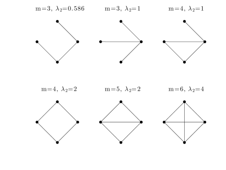
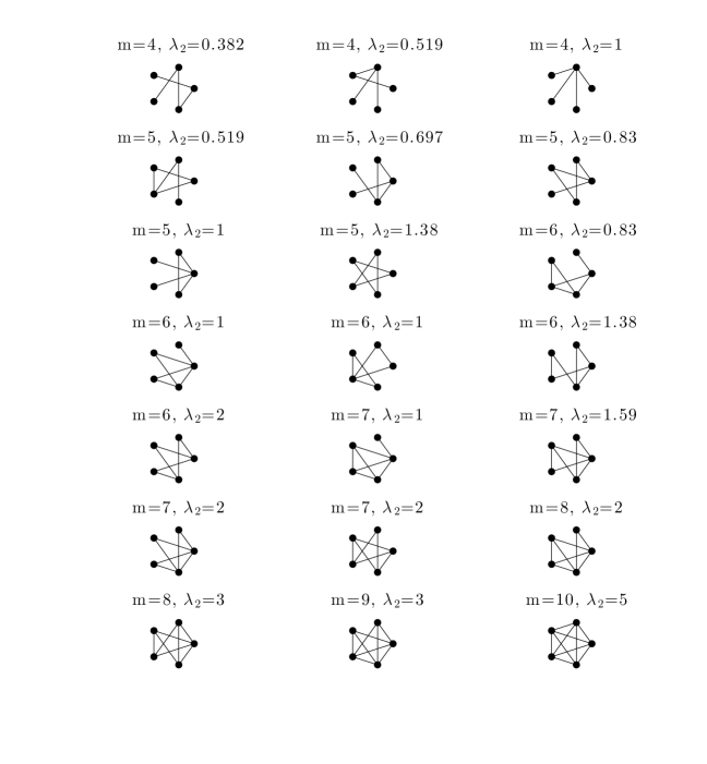
The number of distinct $n$-node, connected, unlabeled graphs for $n=$1, 2, 3, …are 1, 1, 2, 6, 21, 112, 853, 11117, 261080,…(Sloane A001349). In Fig. 1 we plot, for $n=4$ and $n=5$, each of these graphs together with the algebraic connectivity, $\lambda_{2}$. In Fig. 1, we observe that as the number of edges, $m$, is increased, the algebraic connectivity, $\lambda_{2}$, generally increases. Furthermore, for a fixed number of edges, $m$, the algebraic connectivity can vary significantly. For $m=5$, $6$, and $7$, the value of $\lambda_{2}$ varies by a factor $\geq 2$. For $m=5$, the graph with smallest $\lambda_{2}$ has small edge connectivity (and hence small algebraic connectivity) and the graph with largest $\lambda_{2}$ has nodes with equal degree. These small graphs beautifully illustrate the bounds given in §3.

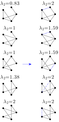
In Fig. 2, we illustrate the effect of adding edges on the algebraic connectivity of a graph by studying (16) where $\|w_{0}\|_{1}=6$ and $\xi=1$. Although the graphs in Fig. 2 are small in size, it is already nontrivial to determine which edge should be added to maximally increase the algebraic connectivity. We observe that for graphs with low algebraic connectivity, a significant gain can be achieved, while the results for graphs with relatively high algebraic connectivity are modest. In the lowermost panel in Fig. 2, the algebraic connectivity remains constant as an edge is added. This follows from the fact that the second eigenvalue for the graph on the left has multiplicity 2 and the interlacing property described in (10).

Figure 2: Targeted data collection for small graphs. (left) The five topologically distinct connected graphs with $n=5$ nodes and $m=6$ edges. (right) For each edgeset on the left, we select one additional edge (blue dashes) so that $\lambda_{2}$ for the perturbed graph is maximal. The algebraic connectivity of each graph is indicated. By Prop. 4.2, a ranking on a dataset represented by a graph on the right is more informative than one from a graph on the left. See §5.1.

Further consideration of the algebraic connectivity for certain families of graphs is considered in Kolokolnikov (2013). Here, it is observed that the greedy algorithm (Algorithm 1) is unable to discover certain small, structured graphs with maximal algebraic connectivity.

5.2 Algebraic connectivity of Erdös-Rényi random graphs and computed nearly-optimal graphs

We consider the Erdös-Rényi random graph model $G(n,p)$ containing graphs with $n$ nodes and edges included with probability $p$, independent from every other edge. The expected number of edges for a graph in $G(n,p)$ is $p\binom{n}{2}$ and the threshold for connectedness is $p_{c}=\frac{\log n}{n}$.

There are several results on the spectrum of the graph Laplacian for Erdös-Rényi graphs, especially in the limit $n\uparrow\infty$; see, for example, (Juhász, 1991; Chung et al., 2003; Feige and Ofek, 2005; Coja-Oghlan, 2007; Jamakovic and Mieghem, 2008; Oliveira, 2009; Chung and Radcliffe, 2011; Kolokolnikov et al., 2013). The algebraic connectivity of Erdös-Rényi, Watts-Strogatz, and Barabási-Albert random graphs has been studied numerically in (Jamakovic and Uhlig, 2007). The algebraic connectivity of a Watts-Strogatz graph is known to have a phase transition (Olfati-Saber et al., 2007).

We will utilize the following elementary upper bound on the algebraic connectivity, analogous to (7), derived using a concentration inequality.

Proposition 5.1

Let $\epsilon>0$ and assume $n$ to be even. With probability at least $1-\epsilon$, the algebraic connectivity, $\lambda_{2}$, of an Erdös-Rényi graph $G(n,p)$ satisfies

$$\lambda_{2}\leq np+4n^{-2}\sqrt{2\log(1/\epsilon)}.$$ (17)

Proof  Choose any subset $U\subset V$ with $|U|=\frac{n}{2}$. Equation (6) implies that $\lambda_{2}\leq\frac{4C}{n}$ where $C\sim\mathcal{B}(\frac{n^{2}}{4},p)$. For $a>0$, we compute

$$\mathrm{pr}\left(\lambda_{2}\geq np+a\right) \leq\mathrm{pr}\left(4C/n\geq np+a\right)=\mathrm{pr}\left(C-pn^{2}/4\geq+an/4\right)\leq\exp\left(-a^{2}n^{4}/32\right)$$

where the last inequality is due to Hoeffding. Setting $a=4n^{-2}\sqrt{2\log(1/\epsilon)}$, we find that $\mathrm{pr}\left(\lambda_{2}\geq np+a\right)\leq\epsilon$ as desired.  
For a random graph $G(n,p)$, the number of edges $m\sim\mathcal{B}(N,p)$ where $N:=n(n-1)/2$. Thus, ${\mathbb{E}}[m]=pN$ and we may restate (17) as: with probability at least $1-\epsilon$,

$$\lambda_{2}\leq\frac{2E[m]}{n-1}+4n^{-2}\sqrt{2\log(1/\epsilon)}.$$ (18)

Indeed, the first term on the right hand side of (18) matches the right hand side of (7).

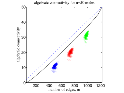
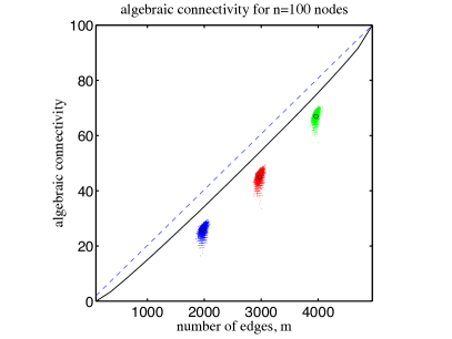
In Figure 3, we plot, for $n=50$ (left) and $n=100$ (right) and $p=.4$ (blue), $p=.6$ (red), and $p=.8$ (green) the value of $m$ vs. $\lambda_{2}$ for 5,000 randomly generated Erdös-Rényi graphs. The mean values obtained are indicated by circles. We use the greedy algorithm described in §3.1 (see Algorithm 1) with initial graph taken to be the path with $n$ vertices, $P_{n}$, to compute nearly-optimal graphs with $n$-nodes and $m$-edges. The solid black line in Figure 3 represents the value of $\lambda_{2}$ for these graphs. Finally, the dashed blue line in Figure 3 represents the upper bound on $\lambda_{2}$ given in (7) (compare also to (18)).

We observe in Figure 3 that nearly-optimal graphs have values which are indeed close to the upper bound on the algebraic connectivity, indicating (i) the upper bound is nearly-tight and (ii) the greedy heuristic (Algorithm 1) produces graphs which are nearly-optimal. We also observe that the algebraic connectivity of nearly-optimal graphs is significantly better than the values for an average Erdös-Rényi random graph.

Figure 3: Algebraic connectivity, $\lambda_{2}$ as a function of $m$ for $50$- and $100$-node graphs. The dashed blue line represents the upper bound on $\lambda_{2}$ given in (7). The solid black line represents the nearly-optimal value of $\lambda_{2}$. Finally, for $p=.4$ (blue), $.6$ (red), and $.8$ (green) we give a scatter plot of $(m,\lambda_{2})$ for 5,000 randomly generated Erdös-Rényi graphs. The mean values obtained are indicated by circles. See §5.2.

5.3 Informativeness of the ranking for the Yahoo! Movie user ratings dataset

In this section, we apply the methodology formulated in §4, to study the Fisher informativeness of the Yahoo! Movie user rating dataset. We show that the addition of targeted edges can significantly improve the informativeness of the movie rating system.

The dataset

The Yahoo! Movie user rating dataset consists of a $7,642\times 11,915$ user-movie matrix where each of the $211,197$ nonzero entries (0.23% sparsity density) is a 1 to 13 rating (yah, ). Each movie was rated by between 1 and 4,238 users (the average number of reviews per movie is 17.7). Each user rated between 10 and 1,632 movies (the average number of reviews made by each reviewer is 27.6). Of the 70,977,655 (movie) pairs $(i,j)$ where $i>j$, there are 5,742,557 for which a user has given a rating to both movies $i$ and $j$ implying that the pairwise comparisons for the raw dataset are 8.1% complete. The majority of movies in the dataset received relatively few reviews, as reported in Table 2.

# times movie reviewed	1	2	3	4	5	6	7	8	9	$\geq 10$
occurrences	4,901	1,882	897	548	398	316	237	202	167	2,367

Table 2: Frequency of reviews for items in the Yahoo! Movie user rating dataset. See §5.2.

The movies which received less than 10 rankings were discarded from the dataset, leaving 2,367 movies, each of which were reviewed by an average of 79.8 users. We then removed 11 users who did not review any of the remaining movies. The remaining 7,631 reviewers reviewed between 1 and 1,220 movies (on average they reviewed 24.8 movies).

Construction of pairwise comparison data from movie-user rating data

Let $\Sigma$ be the set of Yahoo! users, $V$ be the set of all Yahoo! movies and $r_{i}^{\sigma}$ be the rating given to movie $i\in V$ by user $\sigma\in\Sigma$. For each unordered movie pair $\{i,j\}\in V^{2}$, we define

$$\Sigma_{ij}=\{\sigma\in\Sigma\text{ who rated both movies }i\text{ and }j\}.$$

For each movie pair $\{i,j\}\in V^{2}$, we define $w_{ij}$ to be the number of users who have viewed both movies $i$ and $j$, i.e., $w_{ij}=|\Sigma_{ij}|$, and $y_{k}$ to be the average difference in movie reviews, written

$$y_{ij}=\frac{1}{|\Sigma_{ij}|}\sum_{\sigma\in\Sigma_{ij}}(r^{\sigma}_{j}-r^{\sigma}_{i}),\,\,\text{where }\{i,j\}\in V^{2}\text{ and }i<j.$$ (19)

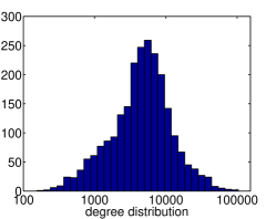
Note that the expression in parenthesis is anti-symmetric in the indices $i$ and $j$ and lies in the interval $[-12,12]$. The choice $i<j$ corresponds to the choice in arc direction in (4). For the Yahoo! Movie user rating dataset, we have $n:=|V|=2,367$, $N:=\binom{n}{2}=2,800,161$, $m:=\|w\|_{0}=1,884,504$, and $M:=\|w\|_{1}=8,322,538$. Thus, there exists at least one comparison for $m/N=67\%$ of the movie pairs. The mean $w$-weighted degree of each node is given by $2\cdot M/n=3,516$. A log-histogram of the $w$-weighted degree distribution of the graph representing the pairwise comparison data is given in Fig. 4 (top left).

$\hat{\phi}_{w}$	Movie Name
4.46	It’s a Wonderful Life (1946)
4.45	Singin’ in the Rain (1952)
4.34	Rear Window (1954)
4.11	24: Season 1 (2002)
3.96	The Longest Day (1962)
3.94	The Man Who Shot Liberty Valance (1962)
3.92	Rebecca (1940)
3.87	Friends - The Complete Fourth Season (1997)
3.79	Lady and the Tramp (1955)
3.79	It Happened One Night (1934)

Figure 4: (top left) A log-histogram of the $w$-weighted degree distribution for the graph representing the Yahoo! movie pairwise comparison data. (top right) A histogram of the residual, $y-B\hat{\phi}_{w}$, where $\hat{\phi}_{w}$ is the least squares ranking. (bottom) Top 10 movies and ranking, $\hat{\phi}_{w}$. See §5.3.

	additional comparisons
method of	original	$.005\%\ M$	$.01\%\ M$
data collection	$\xi=0$	$\xi=416$	$\xi=832$
random	154.38	154.38	154.38
optimal	154.38	298.44	332.78
upper bound (7)	7,035	7,035	7,036

Figure 5: (left) The informativeness of the ranking, $\lambda_{2}(w)$, as a small number ($.01\%\cdot M$) of targeted pairwise comparisons (black) and randomly selected pairwise comparisons (blue) are added. (right) The value of $\lambda_{2}(w)$ for this augmented dataset and the upper bound on $\lambda_{2}$ given in (7). The change in informativeness for randomly added data is unappreciable compared to a 2.2 fold increase for targeted data. See §5.3.

The least squares ranking

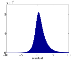
A ranking is obtained by solving the least squares problem, (1), using Matlab’s lsqr function. The top ten movies found are given in Figure 4. The relative residual norm of the least squares estimator, $\hat{\phi}_{w}$, is $\frac{\|B\hat{\phi}_{w}-y\|_{w}}{\|y\|_{w}}=0.53.$ In Fig. 4 (top right), we plot a histogram of the residual, $y-B\hat{\phi}_{w}$. For this pairwise comparison dataset, the normality assumption in Prop. 4.2 is reasonable.

The informativeness of the ranking is $\lambda_{2}(w)=[\text{Var}(\hat{\phi}_{w})]^{-1}=154.38$. This value is small compared to the upper bound given in (7), $\lambda_{2}(w)\leq\frac{2M}{n-1}=7,036$. We next demonstrate that the Fisher information can be significantly improved by the addition of a small number of targeted pairwise comparisons.

Targeted data collection

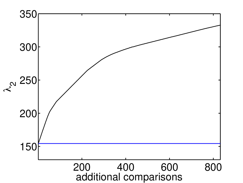
We apply the optimal experimental design approach developed in §4 to improve the Fisher information of the least squares ranking. To approximate the solution of (16), we use the greedy algorithm described in Algorithm 1. The second eigenpair of the graph Laplacian is computed using Matlab’s eigs function, initialized using the eigenvector from the previous iteration. We choose a very modest value of pairwise comparison edges to add, $\xi=.01\%\cdot M=832$ edges. The results are given in Fig. 5. The addition of the targeted pairwise comparisons leads to an increase in the second eigenvalue of the $w$-weighted graph Laplacian by a factor of $2.2$. The maximum increase for the addition of a single pairwise comparison is $\approx 1$, less than the upper bound given in (9). We observe in Fig. 5, that the rate of information increase slows as more pairwise comparisons are added. For a comparison, we also consider the addition of randomly chosen movie pairs. For this modest value of additional edges, $\xi$, the effect of the informativeness of the ranking is unappreciable.

Figure 6: Yahoo! Movie ratings and targeted data collection. (top) A (15% randomly chosen) subset of the pairwise comparison graph for the Yahoo! user-movie database. Nodes represent movies, node size reflects weighted degree (i.e., number of comparisons with other movies), and node color indicates genre (see legend). Edges represent weighted pairwise comparisons colored by edge weights (i.e., number of comparisons). (bottom) Pairwise comparisons targeted for collection to improve the informativeness of the least squares ranking. Targeted comparisons are colored by weight (multiplicity). See §5.3.

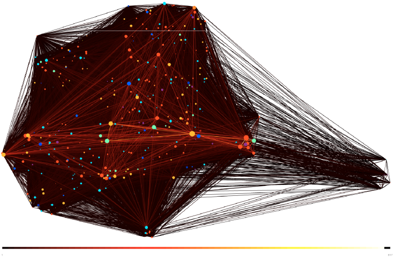
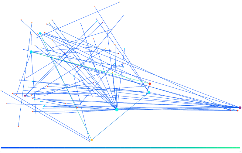
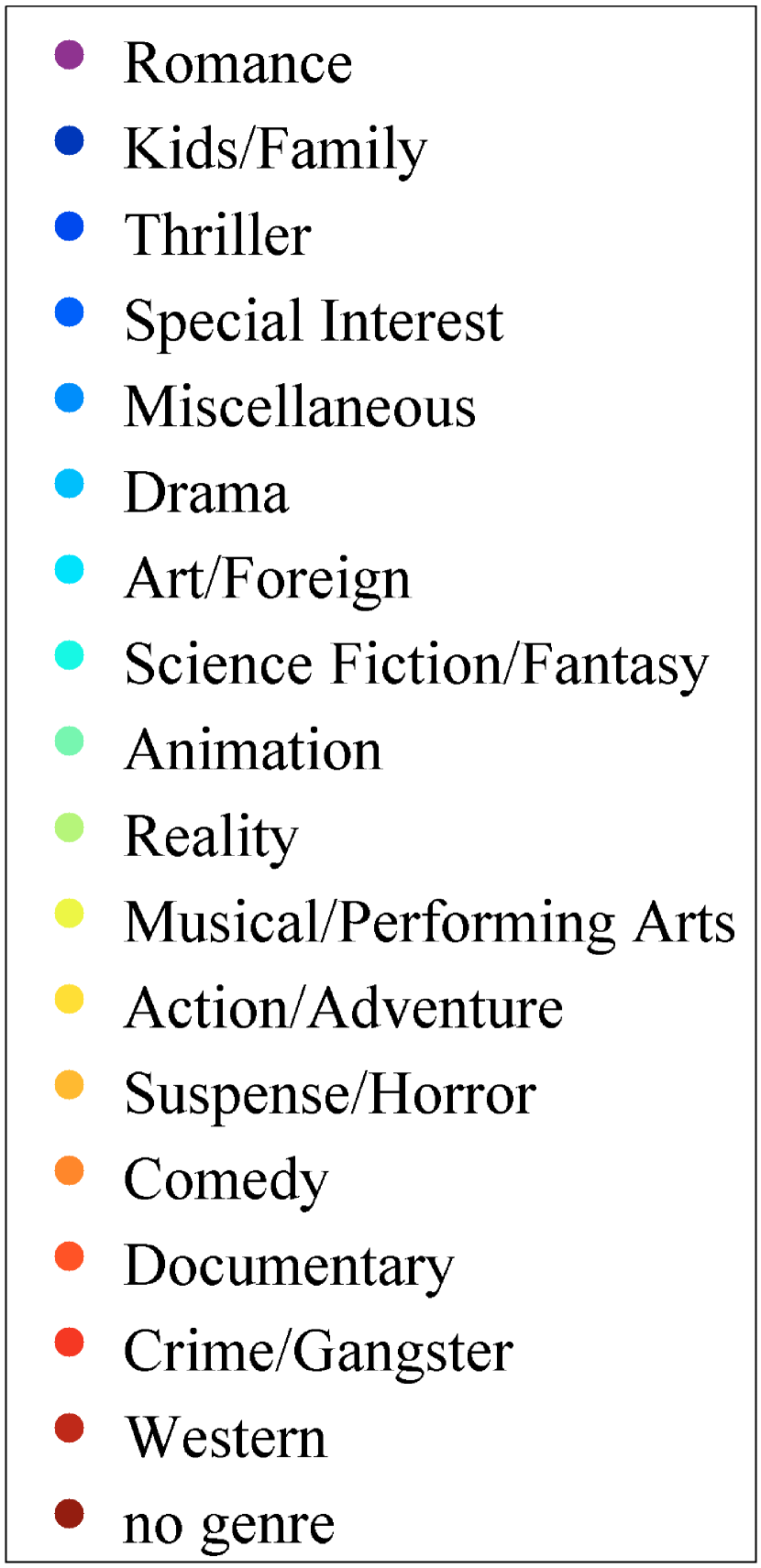
Finally, we use graph visualization via spectral clustering to illustrate the pairwise comparison and targeted data. In Fig. 6(top) we plot the pairwise movie comparisons obtained from the Yahoo! user-movie database. In Fig. 6(bottom) we plot the proposed pairwise comparisons, targeted to improve the informativeness of the rating system. To enhance the readability of the graph representation, we plot only $15\%$ randomly selected nodes ($356$ of $n=2367$) and the interconnecting edges ($45,327$ of $m=1,884,504$). Figure 6(top) was generated as follows. First normalized spectral clustering (based on $k$-means) was used to detect clusters of movies. Next, the Fruchterman-Reingold algorithm was used to generate reasonable positions for the movie clusters and the Kamada-Kawai algorithm was used to place movies within the clusters (Traud et al., 2009). The node placement was obtained using the full dataset. Finally, the weighted graphs were plotted using wgPlot (Wu, 2009). Figure 6(bottom) was then generated using the same node placements as in Figure 6(top).

A comparison of the top and bottom panels of Fig. 6 shows that the primary improvement to informativeness arises from the addition of edges which connects two relatively weakly connected components of the graph. With 4 exceptions, each targeted movie pair is only incremented once; it isn’t generally advantageous to add an edge multiple times.

5.4 2011-12 NCAA Division I football schedule

Recall from §1 that in sports the optimal pairwise data collection problem in equivalent to designing the schedule. In this section, we study the 2011-12 NCAA Division 1 football schedule, downloaded from Massey Ratings. The NCAA Division 1 Football League is divided into the Football Bowl Subdivision (FBS) and Football Championship Subdivision (FCS). The FBS is further decomposed into 12 conferences and the FCS into 15. Of the 246 teams in Division 1, 120 belong to FBS and 126 belong to FCS. Lafayette College is a member of FBS, however every opponent of Lafayette during the 2011-12 season was a member of the FCS. For our purposes, it is more convenient to reclassify Lafayette as a member of FCS and thus, in what follows, FBS has 119 teams and FCS has 127. There were $m=1430$ games among the Division 1 teams and $m=693$ games among the FBS teams.

For static schedules, an important statistic is the the ratio of the total number of games played to the total number of teams. For example, in Major League Baseball (MLB), there are 30 teams, divided into two leagues: the American League (14 teams) and the National League (16 teams). During the regular season, each team plays approximately 160 games, primarily against teams within the same division. Thus, within each league, teams play an average of $160/15\approx 10$ times. With so many games and equal strength of schedule among teams, it is intuitive that the scheduling has little effect on the rankings. And, in fact, MLB simply uses win/loss percentages for ranking purposes. In the NCAA football considered here however, there are 120 teams in the NCAA Football Bowl Subdivision (FBS) and each team plays approximately 6 games per year within FBS. Thus each team only plays roughly $5\%$ of the other teams. There are several rankings for NCAA football which are generated either mathematically or by expert opinion and then aggregated to determine official rankings and select teams to compete in the prestigious end-of-season “bowl games”. The fact that these rankings generally disagree and that none of them is more reliable than the others suggest that none of them are very informative. It is this situation, where there are relatively few games compared to the number of teams, that the schedule has a large effect on the rankings.

Figure 7: 2011-12 NCAA Division 1 (FBS and FCS) football schedule. Graph representation of schedule via spectral clustering by games, top: vertices represent teams, edges represent games, coloring indicates conference membership. bottom: community detection of teams (represented using pie-graphs) reveals that teams primarily play within their own conference. The dashed lines indicate an edge cut which is discussed in the text. See §5.4.

Data visualization via spectral clustering

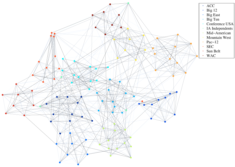
We use the data visualization method described below to demonstrate that NCAA Division 1 teams primarily play against other teams within their own conference. We then show that this clustering of teams by conference results in the graph having poor algebraic connectivity.

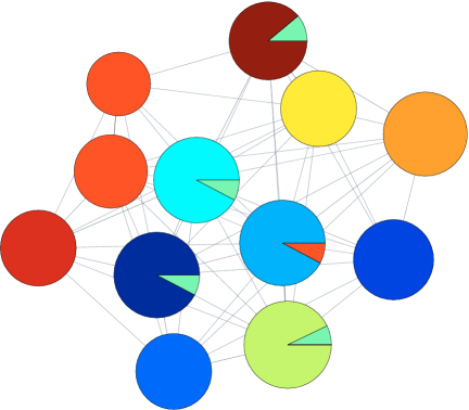
We first use normalized spectral clustering to detect communities within the teams (Shi and Malik, 2000). This, in turn, relies on the $k$-means algorithm where $k$ is the desired number of communities (27 for Division 1 and 12 for Division 1 FBS). Then, using the Matlab toolbox described in (Traud et al., 2009), the Fruchterman-Reingold algorithm finds an optimal placement of the communities and the Kamada-Kawai algorithm is used for the placement of nodes within each community. The mean within-cluster sum of point-to-centroid distances for the $k$-means clustering obtained for the Divsion 1 and Division 1 FBS data is $0.147$ and $0.133$ respectively.

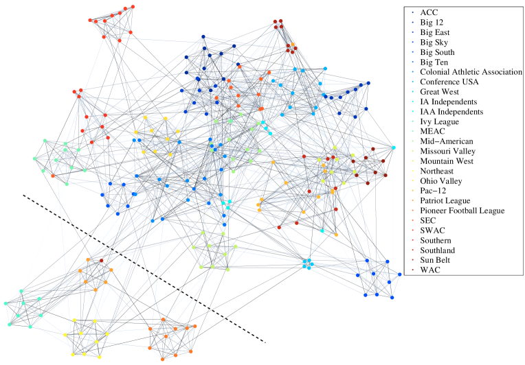
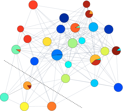
In Figures 7 and 8, we plot the 2011-12 NCAA Division 1 and Division 1 FBS football schedules respectively. In 7(top) and 8(top), the vertices represent teams, the edges represent games, and each vertex (team) is colored by conference membership. In 7(bottom) and 8(bottom), the vertices represent the spectrally clustered communities and the edges represent the community interactions. We observe from Figures 7 and 8 that the teams primarily play within their own conference, which has implications discussed below.

We next compare the value of the algebraic connectivity for these schedules with schedules from Erdös-Rényi random graphs and proposed nearly-optimal schedules.

Figure 8: 2011-12 NCAA Division 1 (only FBS) football schedule. Graph representation of schedule via spectral clustering by games, top: vertices represent teams, edges represent games, coloring indicates conference membership. bottom: community detection of teams (represented using pie-graphs) reveals that teams primarily play within their own conference. See §5.4.

Comparison of NCAA Division 1, Erdös-Rényi random, and nearly-optimal schedules

In the introduction, we noted that there are several common scalar measures of $\text{Var}(\hat{\phi}_{w})$, three of which are given in (3). In this section, we compare these various measures for the NCAA Division 1, Erdös-Rényi random, and nearly-optimal schedules.

More concretely, let $w$ be a given schedule (defining a graph on $n$ vertices) and define the graph Laplacian: $\Delta_{w}:=B^{t}[\text{diag}(w)]B$. Define the following three functions of $w$:

$$J_{E}(w) :=\lambda_{2}(w)$$ (20a)

$$J_{A}(w) :=\left[\frac{1}{n}\text{tr}(\Delta_{w}^{{\dagger}})\right]^{-1}=\left[\frac{1}{n}\sum_{i\geq 2}\frac{1}{\lambda_{i}(w)}\right]^{-1}$$ (20b)

$$J_{D}(w) :=\log[\text{det}(\Delta_{w})]^{\frac{1}{n}}=\frac{1}{n}\sum_{i\geq 2}\log[\lambda_{i}(w)]$$ (20c)

To obtain quantities more comparable to those for the E-optimality condition, for $J_{A}(w)$ we have used the harmonic mean of the eigenvalues rather than the negative of the inverses as in (15b) and for $J_{D}(w)$, we have taken the logarithm of the determinant in (15c). An interpretation of the three quantities defined in (20) in terms of the graph is given in Remark 1.

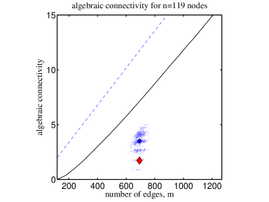
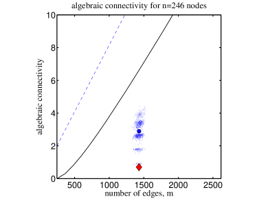
For the Division 1 and Division 1 FBS schedules, we compute the various measures of the quality of schedule given in (20) and record them in Table 3. We also plot $J_{E}(w)$ given in (20a) in Fig. 9 by a red diamond. We next discuss schedules for which we compare the Division 1 and Division 1 FBS schedules in Table 3 and Fig. 9.

The expected number of edges for a $G(n,p)$ Erdös-Rényi random graph is $pN$ where $N:=\binom{n}{2}$. To compare to the football schedules, we take $p=m/N$ and consider the family of random graphs, $G(n,m/N)$. For $n=119$ and $m=693$, we choose $p=m/N\approx 0.0987$ which is approximately $2.5$ times the threshold for connectivity, $p_{c}=\log(n)/n\approx 0.0402$. For $n=246$ and $m=1430$, we choose $p=m/N\approx 0.0475$ which is approximately $2.1$ times the threshold for connectivity, $p_{c}=\log(n)/n\approx 0.0224$. In Table 3, we tabulate the expected values of the three quantities given in (20) for $G(n,m/N)$ graphs, obtained by averaging over a sample size of 1000. Similar to §5.2, in Fig. 9, we give a scatter plot of $(m,\lambda_{2})$ for $G(n,m/N)$ graphs and indicate the mean values with a blue circle.

As in §5.2 and §5.3, we again use the greedy algorithm described in §3.1 (see Algorithm 1) to compute graphs with $n$ nodes and $m$ edges which nearly-maximize $J_{E}=\lambda_{2}$. We then evaluate all three quantities given in (20) for these graphs and tabulate these values in Table 3. The solid black line in Fig. 9 is the best value of $J_{E}=\lambda_{2}$ obtained. Finally, the dashed blue line in Fig. 9 represents the upper bound on $\lambda_{2}$ given in (7).

We observe in Fig. 9 and Table 3 that the schedules which nearly-maximize $J_{E}(w)=\lambda_{2}$ have significantly larger values of $J_{E}$ than the NCAA Division 1 and Division 1 FBS schedules. In fact, the NCAA schedules have worse values than schedules associated with Erdös-Rényi random graphs of the same size. Furthermore, we show in Table 3 that schedules which maximize $J_{E}$ also have larger values of $J_{A}$ and $J_{D}$. That is, the schedules which are good in the sense of E-optimality are also good schedules in the sense of D- and E-optimality as defined in (3).

The reason for the relatively poor value of $J_{E}(w)=\lambda_{2}$ for the NCAA Division 1 and Division 1 FBS schedules can be understood from Figures 7 and 8. Figures 7 and 8 reveal that teams primarily play within their own conference. This results in a small edge cut between a conference (or set of conferences) and its vertex complement, which, by (6), implies a small algebraic connectivity. For example, the edge cut indicated by the dashed line in Fig. 7 (entire NCAA Division 1 schedule) results in an upper bound on the algebraic connectivity of 1.297. The edge cut obtained by considering the set consisting of teams in the SWAC conference yields an upper bound equal to 1.043. Both of these bounds are already less than the expected value of $\lambda_{2}$ for Erdös-Rényi random graphs of comparable size (compare with the top part of the first column in Table 3). To summarize, the NCAA primarily schedules games among teams within the same conferences and this reduces the informativeness of the rankings.

The schedule design methodology advocated in Eq. (16) is flexible in the following two senses: (i) The optimal schedules contain symmetry with respect to permutations in the seeding of the teams. This problem has been studied previously for tournaments; see the discussion in §2. (ii) The optimal schedule is not time dependent and thus the scheduling of future games does not depend on past game performances, i.e., the schedule is completely known before the season begins and the games may be played in any order. These properties can be exploited in the further design of the schedule.

Figure 9: A comparison of $J_{E}(w)=\lambda_{2}$ defined in (20a) for the Division 1 and Division 1 FBS schedules, Erdös-Rényi random schedules, and schedules which nearly-maximize $\lambda_{2}$. The red diamonds represents the 2011 NCAA Division 1 (right) and Division 1 FBS (left) football schedule. The solid black lines represent the nearly-optimal values of $\lambda_{2}$ obtained for $n=119$ (left) and $n=246$ (right). The dashed blue lines represent the upper bound on $\lambda_{2}$ given in (7). The blue dots represent a scatter plot of $(m,\lambda_{2})$ for 1,000 randomly generated Erdös-Rényi graphs, $G(n,m/N)$. The mean values are indicated by blue circles. See §5.4.

	$J_{E}(w)$ in (20a)	$J_{A}(w)$ in (20b)	$J_{D}(w)$ in (20c)
Div. 1 FBS and FCS	0.7015	8.780	2.363
Erdös-Rényi, $n=246$	2.892	9.681	2.358
E-optimal design, $n=246$	6.630	10.71	2.403
Div. 1 FBS	1.725	9.634	2.372
Erdös-Rényi, $n=119$	3.497	9.911	2.361
E-optimal design, $n=119$	7.142	10.92	2.402

Table 3: A comparison of the three objective functions defined in (20) for the Division 1 and Division 1 FBS schedules, Erdös-Rényi random schedules, and schedules which nearly-maximize $J_{E}(w)=\lambda_{2}$. Schedules which nearly-maximize $J_{E}(w)=\lambda_{2}$ also have larger values of $J_{A}$ and $J_{D}$ than the comparison schedules. See §5.4

5.5 Synthetic data experiment on the 2011-2012 NCAA Division 1 FBS graph

To further illustrate and test our proposed active learning method, we again consider the graph generated in §5.4 from the 2011-12 NCAA Division I Football Bowl Subdivision (FBS) schedule with $n=119$ nodes and $m=693$ edges, as shown in Figure 8. We take as ground truth rating, $\phi$, a normally distributed vector with mean zero and variance, $\sigma^{2}=1$. The ground truth rating, $\phi$, is used to generate new data according to the normal model (11) with $\sigma^{2}=5$. With this data, we solve (12) to obtain a least squares estimate, $\hat{\phi}_{w_{0}}$. We compute $\|\hat{\phi}_{w_{0}}-\phi\|_{2}=17.31$ and $K(\phi_{w_{0}},\phi)=0.35$. Here, the Kendall-$\tau$ rank distance between two rankings $\phi_{1}$ and $\phi_{2}$ is defined as the fraction of pairwise disagreements between the rankings,

$$K(\phi_{1},\phi_{2}):=\frac{\#\{(i,j)\colon i>j,\ \phi_{1}(i)<\phi_{1}(j),\text{ and }\phi_{2}(i)>\phi_{2}(j)\}}{n(n-1)/2}.$$ (21)

Figure 10: A comparison of ranking errors and algebraic connectivity, a measure of the informativeness of the ranking, for two data collection strategies: the proposed active sampling method (black and green) and random sampling (red and blue). (left) The $L^{2}$-error, $\|\hat{\phi}_{\xi}-\phi\|_{2}$ between the estimated and ground truth rankings. (center) The Kendall-$\tau$ rank distance, (21), between the estimated and ground truth rankings. (right) The algebraic connectivity of the graph representing the dataset. See §5.5.

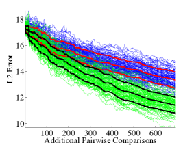
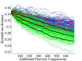
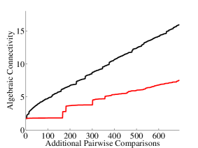
We then consider enhancing the dataset by adding $\xi$ more pairwise comparisons. Using the enhanced dataset, we compute an estimate of the ranking, $\hat{\phi}_{\xi}$, and, as $\hat{\phi}_{\xi}$ is an unbiased estimate of $\phi$, expect $\|\hat{\phi}_{\xi}-\phi\|_{2}$ to diminish as $\xi\to\infty$. We choose $\xi=693$, so that the number of pairwise comparisons (games played) is doubled. As in §5.3, we add pairwise comparisons either by the greedy algorithm (Algorithm 1) or by random selection. As with the data collected on the initial graph, the new data are collected according to the normal model (11) with $\sigma^{2}=5$. In Fig. 10(left), we plot the number of additional pairwise comparisons vs. the $L^{2}$-error, $\|\hat{\phi}_{\xi}-\phi\|_{2}$, for an ensemble of ranking estimates determined using the two data collection strategies. The (thin) blue and green lines represent the error for 100 instances of data collection using the random and greedy methods respectively. The (thick) red and black lines represent the mean and mean plus/minus one standard deviation for each of the two data collection strategies. For $\xi=693$, the mean $L^{2}$-error for the proposed data collection strategy is 11.38 while the mean error for the random data collection strategy is 13.32, representing a reduction in error of $34\%$ and $23\%$ respectively. In Fig. 10(center), we plot the number of additional pairwise comparisons vs. the Kendall-$\tau$ rank distance, $K(\phi,\phi_{\xi})$, for these two data collection strategies. For $\xi=693$, the mean distance for the proposed data collection strategy is .27 while the mean error for the random data collection strategy is 0.30, representing a reduction in distance of $22\%$ and $14\%$ respectively. In Fig. 10(right), we plot the algebraic connectivity, a measure of the informativeness of the ranking, vs. the number of additional pairwise comparisons. The black (red) line is the algebraic connectivity for the graph representing the dataset where edges are added using the greedy algorithm (random sampling). Supported by Propositions 4.1 and 4.2, the dataset represented by a graph with larger algebraic connectivity is more informative and thus produces a ranking estimate with greater fidelity to the ground truth estimate.

6 Discussion and future directions

We have applied methods from optimal experiment design to provide a new framework for data collection for more informative statistical rankings. At the heart of this framework is a bi-level optimization problem (2) where the inner problem is to determine the unbiased ranking for a given schedule and the outer problem is to identify data which maximizes the Fisher information of the ranking. For the least-squares estimate, the outer problem decouples from the inner problem and reduces to an eigenvalue optimization problem. For the E-optimality criterion for the Fisher information, this is the problem of finding an edge weight $w\in\mathbb{Z}_{+}^{N}$, such that the $w$-weighted graph Laplaican has large second eigenvalue (16). This can be interpreted as finding a multigraph with large algebraic connectivity, a problem which has been well-studied in graph theory. In the case of NCAA Division 1 football, we demonstrated in §5.4 and Table 3 that the nearly-optimal data collection strategy in the sense of E-optimality is also a good startegy in the sense of D- and A-optimality; the choice of scalar function $f\colon\mathbb{S}_{+}^{n}\to\mathbb{R}$ as defined in (2) does not strongly effect the optimal data collection strategy (see Remark 1 for a further discussion of these optimality criteria). Furthermore, in §5.5, we demonstrate using a synthetically constructed dataset on this graph that the ranking estimate obtained via active sampling has greater fidelity to ground truth than the ranking estimate obtained via random sampling.

There are several applications in, e.g., social networking, game theory, and e-commerce, where improved data collection could potentially benefit ranking. In particular, for the Yahoo! Movie user ratings dataset (considered in §5.3), we have shown that the informativeness of ranking can be increased by a factor of $2.2$ if just $.01\%$ of additional optimally-targeted pairwise comparisons are added to the dataset. In contrast, if the same amount of random data is added, there is an unappreciable effect on the informativeness of the ranking. For this application, the data collection problem could be more carefully modeled. Here, the pairwise comparison data is constructed from user rating data and thus any targeted pairwise comparison addition must be solicited from a user. Since the number of pairwise comparisons for which a particular reviewer adds when a new movie is reviewed is equal to the number of previous reviews that user has contributed, it may make sense to solicit additional reviews from users with many previous reviews. That is, the propagation of information from the user reviews to the pairwise comparison data in (19) should also be considered.

We have focused on optimal data collection for improved rankings, neglecting several important factors including the cost of data collection and potential constraints on what data may be collected. There are two simple extensions to our method which may be employed to accommodate these additional factors. The cost of data collection could be incorporated by either adding a penalization term in (16) or by incorporating additional weights into the norm used to compute $\lambda_{2}$ in (16). Data collection constraints may be handled by explicitly forbidding certain edge weights to be incremented in the greedy Algorithm 1 for targeting data collection.

The least-squares ranking estimate (1) is referred to as HodgeRank by some authors Jiang et al. (2010); Xu et al. (2011), since the Hodge decomposition implies that the residual in (1), $r=B\phi-y$, can be further decomposed into two orthogonal components: (1) a divergence-free component which consists of 3-cycles and (2) a harmonic component which consists of longer cycles Jiang et al. (2010); Hirani et al. (2011). In fact, Jiang et al. (2010) argues that a dataset which has a large harmonic component is inherently inconsistent and does not have a reasonable ranking. The harmonic component lies in the kernel of the graph Helmholtzian with dimension given by the first Betti number of the associated simplical complex. Optimal reduction of the first Betti number may provide an alternative approach to improving the informativeness of the least squares ranking.

Recently, Masuda et al. (2013) developed an algorithm for removing nodes from a graph to increase the algebraic connectivity. This algorithm could be used to prune the alternatives in a dataset to increase the informativeness of a ranking.

Finally, we are interested in extending this work to nonlinear ranking methods, including robust estimators (Osting et al., 2013b), random walker methods (Callaghan et al., 2007), Perron-Frobenius eigenvalue methods (Keener, 1993; Langville and Meyer, 2012), and Elo methods (Elo, 1978; Glickman, 1995; Langville and Meyer, 2012).

Acknowledgments

We thank Lawrence Carin, Jérôme Darbon, Mark L. Green, and Yuan Yao for useful discussions. B. Osting is supported by NSF DMS-1103959. C. Brune is supported by ONR grants N00014-10-10221 and N00014-12-10040. S. Osher is supported by ONR N00014-08-1-1119, N00014-10-10221, and NSF DMS-0914561.

References

- (1) Yahoo! Webscope dataset: ydata-ymovies-user-movie-ratings-content-v1_0. http://webscope.sandbox.yahoo.com. accessed: 10/5/2011.
- Ailon (2012) N. Ailon. An active learning algorithm for ranking from pairwise preferences with an almost optimal query complexity. J. Mach. Learn. Res., 13:137–164, 2012.
- Ailon et al. (2011) N. Ailon, R. Begleiter, and E. Ezra. Active learning using smooth relative regret approximations with applications. arXiv preprint arXiv:1110.2136, 2011.
- Barrow et al. (2013) D. Barrow, I. Drayer, P. Elliott, G. Gaut, and B. Osting. Ranking rankings: an empirical comparison of the predictive power of sports ranking methods. J. Quantitative Analysis in Sports, 9(2):187–202, 2013.
- Ben-Naim and Hengartner (2007) E. Ben-Naim and N. W. Hengartner. Efficiency of competitions. Phys. Rev. E, 76:026106, 2007.
- Biyikoglu et al. (2007) T. Biyikoglu, J. Leydold, and P. F. Stadler. Laplacian Eigenvectors of Graphs. Springer, 2007.
- Björner et al. (1991) A. Björner, L. Lovász, and P. W. Shor. Chip-firing games on graphs. European J. Combin, 12(4), 1991.
- Boumal et al. (2012) N. Boumal, A. Singer, P.-A. Absil, and V. D. Blondel. Cramér-Rao bounds for synchronization of rotations. arXiv preprint arXiv:1211.1621, 2012.
- Boyd et al. (2004) S. Boyd, P. Diaconis, and L. Xiao. Fastest mixing Markov chain on a graph. SIAM Review, 46(4):667–689, 2004.
- Callaghan et al. (2007) T. Callaghan, P. J. Mucha, and M. A. Porter. Random walker ranking for NCAA Division I-A football. American Mathematical Monthly, 114(9):761–777, 2007.
- Chung (1997) F. R. K. Chung. Spectral Graph Theory. AMS, 1997.
- Chung and Radcliffe (2011) F. R. K. Chung and M. Radcliffe. On the spectra of general random graphs. Electronic Journal of Combinatorics, 18(1):215–229, 2011.
- Chung et al. (2003) F. R. K. Chung, L. Lu, and V. H. Vu. The spectra of random graphs with given expected degrees. Internet Mathematics, 1:257–275, 2003.
- Chung and Haber (2012) M. Chung and E. Haber. Experimental design for biological systems. SIAM J. Control Optim., 50(1):471–489, 2012.
- Coja-Oghlan (2007) A. Coja-Oghlan. On the Laplacian eigenvalues of . Combinatorics, Probability, & Computing, 16(6):923–946, 2007.
- David (1963) H. A. David. The Method of Paired Comparisons. Charles Griffin & Co., 1963.
- DiStefano 3rd (1976) J. J. DiStefano 3rd. Tracer experiment design for unique identification of nonlinear physiological systems. Am. J. Physiol., 230(2):476–485, 1976.
- D’Souza (2010) C. D’Souza. Optimising a tournament for use with ranking algorithms. preprint, 2010.
- Eichhorn et al. (2010) A. Eichhorn, P. Ni, and R. Eg. Randomised pair comparison: an economic and robust method for audiovisual quality assessment. In Proceedings of the 20th international workshop on Network and operating systems support for digital audio and video, pages 63–68. ACM, 2010.
- Elo (1978) A. Elo. The Rating of Chessplayers, Past and Present. Arco Pub., 1978.
- Fallat et al. (2003) S. M. Fallat, S. Kirkland, and S. Pati. On graphs with algebraic connectivity equal to minimum edge density. Linear Algebra and its Applications, 373:31–50, 2003.
- Fedorov (1972) V. V. Fedorov. Theory of Optimal Experiments. Academic Press, 1972.
- Feige and Ofek (2005) U. Feige and E. Ofek. Spectral techniques applied to sparse random graphs. Random Structures & Algorithms, 27(2):251–275, 2005.
- Fiedler (1973) M. Fiedler. Algebraic connectivity of graphs. Czech. Math. J., 23:298–305, 1973.
- Ghosh and Boyd (2006a) A. Ghosh and S. Boyd. Upper bounds on algebraic connectivity via convex optimization. Linear Algebra and its Applications, 418:693–707, 2006a.
- Ghosh and Boyd (2006b) A. Ghosh and S. Boyd. Growing well-connected graphs. Proc. IEEE Conf. Decision & Control, 2006b.
- Ghosh et al. (2008) A. Ghosh, S. Boyd, and A. Saberi. Minimizing effective resistance of a graph. SIAM Review, 50(1):37–66, 2008.
- Glickman (1995) M. E. Glickman. A comprehensive guide to chess ratings. American Chess Journal, 3, 1995.
- Glickman (2005) M. E. Glickman. Adaptive paired comparison design. Journal of Statistical Planning and Inference, 127:279–293, 2005.
- Glickman (2008) M. E. Glickman. Bayesian locally optimal design of knockout tournaments. Journal of Statistical Planning and Inference, 138(7):2117 – 2127, 2008.
- Grimmett (2010) G. Grimmett. Probability on Graphs: Random Processes on Graphs and Lattices. Cambridge University Press, 2010.
- Haber et al. (2008) E. Haber, L. Horesh, and L. Tenorio. Numerical methods for experimental design of large-scale linear ill-posed inverse problems. Inverse Problems, 24:055012, 2008.
- Hirani et al. (2011) A. N. Hirani, K. Kalyanaraman, and S. Watts. Least squares ranking on graphs. arXiv:1011.1716v4, 2011.
- Horesh et al. (2011) L. Horesh, E. Haber, and L. Tenorio. Optimal experimental design for the large-scale nonlinear ill-posed problem of impedance imaging. In L. Biegler et al, editor, in: Large-Scale Inverse Problems and Quantification of Uncertainty. Wiley Ser. Comp. Stat., 2011.
- Horn and Johnson (1990) R. A. Horn and C. R. Johnson. Matrix Analysis. Cambridge University Press, 1990.
- Jamakovic and Mieghem (2008) A. Jamakovic and P. Van Mieghem. On the robustness of complex networks by using the algebraic connectivity. In Networking 2008 Ad Hoc and Sensor Networks, Wireless Networks, Next Generation Internet, pages 183–194. Springer, 2008.
- Jamakovic and Uhlig (2007) A. Jamakovic and S. Uhlig. On the relationship between the algebraic connectivity and graph’s robustness to node and link failures. In Proceedings of the 3rd EURO-NGI Conference on Next Generation Internet Network, 2007.
- Jamieson and Nowak (2011) K. G. Jamieson and R. D. Nowak. Active ranking using pairwise comparisons. In Neural Information Processing Systems (NIPS), pages 2240–2248, 2011.
- Jamieson and Nowak (2012) K. G. Jamieson and R. D. Nowak. Active ranking in practice: General ranking functions with sample complexity bounds. 2012.
- Jiang et al. (2010) X. Jiang, L.-H. Lim, Y. Yao, and Y. Ye. Statistical ranking and combinatorial Hodge theory. Math. Program. Ser. B, 127(1):203–244, 2010.
- Juhász (1991) F. Juhász. The asymptotic behaviour of Fiedler’s algebraic connectivity for random graphs. Discrete Mathematics, 96(1):59–63, 1991.
- Keener (1993) J. P. Keener. The Perron-Frobenius theorem and the ranking of football teams. SIAM Review, 35(1):80–93, 1993.
- Kolokolnikov (2013) T. Kolokolnikov. Maximizing algebraic connectivity for certain families of graphs. submitted, 2013.
- Kolokolnikov et al. (2013) T. Kolokolnikov, B. Osting, and J. Von Brecht. Algebraic connectivity of Erdös-Rényi graphs near the connectivity threshold. submitted, 2013.
- Krause et al. (2008) A. Krause, A. Singh, and C. Guestrin. Near-optimal sensor placements in Gaussian processes: Theory, efficient algorithms and empirical studies. The Journal of Machine Learning Research, 9:235–284, 2008.
- Langville and Meyer (2012) A. N. Langville and C. D. Meyer. Who’s #1?: The Science of Rating and Ranking. Princeton University Press, 2012.
- Masuda et al. (2013) N. Masuda, T. Fujie, and K. Murota. Application of semidefinite programming to maximize the spectral gap produced by node removal. In Complex Networks IV, pages 155–163. Springer, 2013.
- Melas (2006) V. B. Melas. Functional approach to optimal experimental design. Springer, 2006.
- Mohar (1991) B. Mohar. The Laplacian spectrum of graphs. In Graph Theory, Combinatorics, and Applications, volume 2, pages 871–898. Wiley, 1991.
- Mosk-Aoyama (2008) D. Mosk-Aoyama. Maximum algebraic connectivity augmentation is NP-hard. Operations Research Letters, 36(6):677–679, 2008.
- Olfati-Saber et al. (2007) R. Olfati-Saber, A. Fax, and R. M. Murray. Consensus and cooperation in networked multi-agent systems. Proceedings of the IEEE, 95(1):215–233, 2007.
- Oliveira (2009) R. I. Oliveira. Concentration of the adjacency matrix and of the Laplacian in random graphs with independent edges. arXiv:0911.0600v2, 2009.
- Osting et al. (2013a) B. Osting, C. Brune, and S. Osher. Enhanced statistical rankings via targeted data collection. JMLR, W&CP, 28(1):489–497, 2013a.
- Osting et al. (2013b) B. Osting, J. Darbon, and S. Osher. Statistical ranking using the -norm on graphs. AIMS J. Inverse Problems and Imaging, 7(3):907–926, 2013b.
- Pukelsheim (2006) F. Pukelsheim. Optimal Design of Experiments. SIAM, 2006.
- Quinn and Keough (2002) G. P. Quinn and M. J. Keough. Experimental design and analysis for biologists. Cambridge University Press, Cambridge, UK, 2002.
- Scarf and Yusof (2011) P. A. Scarf and M. M. Yusof. A numerical study of tournament structure and seeding policy for the soccer world cup finals. Statistica Neerlandica, 65(1):43–57, 2011.
- Seeger and Nickisch (2011) M. Seeger and H. Nickisch. Large scale Bayesian inference and experimental design for sparse linear models. SIAM Journal of Imaging Sciences, 4(1):166–199, 2011.
- Shi and Malik (2000) J. Shi and J. Malik. Normalized cuts and image segmentation. IEEE Transactions on Pattern Analysis and Machine Intelligence, 22(8):888–905, 2000.
- Silva and Carin (2012) J. Silva and L. Carin. Active learning for online Bayesian matrix factorization. accepted paper at the 18th ACM SIGKDD conference on knowledge discovery and data mining, Beijing, China, 2012.
- Sun et al. (2004) J. Sun, S. Boyd, L. Xiao, and P. Diaconis. The fastest mixing Markov process on a graph and a connection to a maximum variance unfolding problem. SIAM Review, 48:2006, 2004.
- Traud et al. (2009) A. L. Traud, C. Frost, P. J. Mucha, and M. A. Porter. Visualization of communities in networks. Chaos, 19:041104, 2009.
- Vu et al. (2009) T. Vu, A. Altman, and Y. Shoham. On the complexity of schedule control problems for knockout tournaments. In Proc. of 8th Int. Conf. on Autonomous Agents and Multiagent Systems (AA-MAS 2009) in Budapest, Hungary, 2009.
- Wang and Mieghem (2008) H. Wang and P. Van Mieghem. Algebraic connectivity optimization via link addition. In Bionetics 2008, Hyogo, Japan, 2008.
- Wauthier et al. (2013) F. L. Wauthier, M. I. Jordan, and N. Jojic. Efficient ranking from pairwise comparisons. In Proceedings of the 30th International Conference on Machine Learning (ICML), 2013.
- Wu (2009) M. Wu. wgPlot. http://www.mathworks.com/matlabcentral/fileexchange/24035, 2009.
- Xu et al. (2011) Q. Xu, Y. Yao, T. Jiang, Q. Huang, B. Yan, and W. Lin. Random partial paired comparison for subjective video quality assessment via HodgeRank. In ACM Multimedia, 2011.
- Xu et al. (2012) Q. Xu, Q. Huang, and Y. Yao. Online crowdsourcing subjective image quality assessment. In Proceedings of the 20th ACM international conference on Multimedia, pages 359–368. ACM, 2012.