Low Rank Approximation and Regression in
Input Sparsity Time

Abstract

We design a new distribution over ${\mathrm{poly}}(r\varepsilon^{-1})\times n$ matrices $S$ so that for any fixed $n\times d$ matrix $A$ of rank $r$, with probability at least $9/10$, ${\|SAx\|}_{2}=(1\pm\varepsilon){\|Ax\|}_{2}$ simultaneously for all $x\in\mathbb{R}^{d}$. Such a matrix $S$ is called a subspace embedding. Furthermore, $SA$ can be computed in $O(\operatorname{\mathtt{nnz}}(A))$time, where $\operatorname{\mathtt{nnz}}(A)$ is the number of non-zero entries of $A$. This improves over all previous subspace embeddings, which required at least $\Omega(nd\log d)$ time to achieve this property. We call our matrices $S$ sparse embedding matrices.

Using our sparse embedding matrices, we obtain the fastest known algorithms for overconstrained least-squares regression, low-rank approximation, approximating all leverage scores, and $\ell_{p}$-regression:

• to output an $x^{\prime}$ for which

  $${\|Ax^{\prime}-b\|}_{2}\leq(1+\varepsilon)\min_{x}{\|Ax-b\|}_{2}$$

  for an $n\times d$ matrix $A$ and an $n\times 1$ column vector $b$, we obtain an algorithm running in $O(\operatorname{\mathtt{nnz}}(A))+\tilde{O}(d^{3}\varepsilon^{-2})$ time, and another in $O(\operatorname{\mathtt{nnz}}(A)\log(1/\varepsilon))+\tilde{O}(d^{3}\log(1/\varepsilon))$ time. (Here $\tilde{O}(f)=f\cdot\log^{O(1)}(f)$.)

• to obtain a decomposition of an $n\times n$ matrix $A$ into a product of an $n\times k$ matrix $L$, a $k\times k$ diagonal matrix $D$, and an $n\times k$ matrix $W$, for which

  $${\|A-LDW^{\top}\|}_{F}\leq(1+\varepsilon){\|A-A_{k}\|}_{F},$$

  where $A_{k}$ is the best rank-$k$ approximation, our algorithm runs in

  $$O(\operatorname{\mathtt{nnz}}(A))+\tilde{O}(nk^{2}\varepsilon^{-4}+k^{3}\varepsilon^{-5})$$

  time.

• to output an approximation to all leverage scores of an $n\times d$ input matrix $A$ simultaneously, with constant relative error, our algorithms run in $O(\operatorname{\mathtt{nnz}}(A)\log n)+\tilde{O}(r^{3})$ time.

• to output an $x^{\prime}$ for which

  $${\|Ax^{\prime}-b\|}_{p}\leq(1+\varepsilon)\min_{x}{\|Ax-b\|}_{p}$$

  for an $n\times d$ matrix $A$ and an $n\times 1$ column vector $b$, we obtain an algorithm running in $O(\operatorname{\mathtt{nnz}}(A)\log n)+{\mathrm{poly}}(r\varepsilon^{-1})$ time, for any constant $1\leq p<\infty$.

We optimize the polynomial factors in the above stated running times, and show various tradeoffs. Finally, we provide preliminary experimental results which suggest that our algorithms are of interest in practice.

1 Introduction

A large body of work has been devoted to the study of fast randomized approximation algorithms for problems in numerical linear algebra. Several well-studied problems in this area include least squares regression, low rank approximation, and approximate computation of leverage scores. These problems have many applications in data mining [5], recommendation systems [19], information retrieval [45], web search [1, 35], clustering [15, 38], and learning mixtures of distributions [34, 2]. The use of randomization and approximation allows one to solve these problems much faster than with deterministic methods.

For example, in the overconstrained least-squares regression problem, we are given an $n\times d$ matrix $A$ of rank $r$ as input, $n\gg d$, together with an $n\times 1$ column vector $b$. The goal is to output a vector $x^{\prime}$ so that with high probability, $\|Ax^{\prime}-b\|_{2}\leq(1+\varepsilon)\min_{x}\|Ax-b\|_{2}$. The minimizing vector $x^{*}$ can be expressed in terms of the Moore-Penrose pseudoinverse $A^{-}$ of $A$, namely, $x^{*}=A^{-}b$. If $A$ has full column rank, this simplifies to $x^{*}=(A^{\top}A)^{-1}A^{\top}b$. This minimizer can be computed deterministically in $O(nd^{2})$ time, but with randomization and approximation, this problem can be solved in $O(nd\log d)+{\mathrm{poly}}(d\varepsilon^{-1})$ time [50, 26], which is much faster for $d\ll n$ and $\epsilon$ not too small. The generalization of this problem to $\ell_{p}$-regression is to output a vector $x^{\prime}$ so that with high probability $\|Ax^{\prime}-b\|_{p}\leq(1+\varepsilon)\min_{x}\|Ax-b\|_{p}$. This can be solved exactly using convex programming, though with randomization and approximation it is possible to achieve $O(nd\log n)+{\mathrm{poly}}(d\varepsilon^{-1})$ time [9] for any constant $p$, $1\leq p<\infty$.

Another example is low rank approximation. Here we are given an $n\times n$ matrix (which can be generalized to $n\times d$) and an input parameter $k$, and the goal is to find an $n\times n$ matrix $A^{\prime}$ of rank at most $k$ for which $\|A^{\prime}-A\|_{F}\leq(1+\varepsilon)\|A-A_{k}\|_{F}$, where for an $n\times n$ matrix $B$, $\|B\|^{2}_{F}\equiv\sum_{i=1}^{n}\sum_{j=1}^{n}B_{i,j}^{2}$ is the squared Frobenius norm, and $A_{k}\equiv\operatorname{\mathrm{argmin}}_{\operatorname{\mathtt{rank}}B\leq k}\|A-B\|_{F}$. Here $A_{k}$ can be computed deterministically using the singular value decomposition in $O(n^{3})$ time. However, using randomization and approximation, this problem can be solved in $O(\operatorname{\mathtt{nnz}}(A)\cdot(k/\varepsilon+k\log k)+n\cdot{\mathrm{poly}}(k/\varepsilon))$ time[50, 10], where $\operatorname{\mathtt{nnz}}(A)$ denotes the number of non-zero entries of $A$. The problem can also be solved using randomization and approximation in $O(n^{2}\log n)+n\cdot{\mathrm{poly}}(k/\varepsilon)$ time [50], which may be faster than the former for dense matrices and large $k$.

Another problem we consider is approximating the leverage scores. Given an $n\times d$ matrix $A$ with $n\gg d$, one can write $A=U\Sigma V^{\top}$ in its singular value decomposition, where the columns of $U$ are the left singular vectors, $\Sigma$ is a diagonal matrix, and the columns of $V$ are the right singular vectors. Although $U$ has orthonormal columns, not much can be immediately said about the squared lengths $\|U_{i}\|_{2}^{2}$ of its rows. These values are known as the leverage scores, and measure the extent to which the singular vectors of $A$ are correlated with the standard basis. The leverage scores are basis-independent, since they are equal to the diagonal elements of the projection matrix onto the span of the columns of $A$; see [21] for background on leverage scores as well as a list of applications. The leverage scores will also play a crucial role in our work, as we shall see. The goal of approximating the leverage scores is to, simultaneously for each $i\in[n]$, output a constant factor approximation to $\|U_{i}\|_{2}^{2}$. Using randomization, this can be solved in $O(nd\log n+d^{3}\log d\log n)$ time [21].

There are also solutions for these problems based on sampling. They either get a weaker additive error [27, 45, 3, 16, 17, 18, 22, 49, 13], or they get bounded relative error but are slow [14, 23, 24, 25]. Many of the latter algorithms were improved independently by Deshpande and Vempala [14] and Sarlós [50], and in followup work [26, 44, 37]. There are also solutions based on iterative and conjugate-gradient methods, see, e.g., [52], or [54] as recent examples. These methods repeatedly compute matrix-vector products $Ax$ for various vectors $x$; in the most common setting, such products require $\Theta(\operatorname{\mathtt{nnz}}(A))$ time. Thus the work per iteration of these methods is $\Theta(\operatorname{\mathtt{nnz}}(A))$, and the number of iterations $N$ that are performed depends on the desired accuracy, spectral properties of $A$, numerical stability issues, and other concerns, and can be large. A recent survey suggests that $N$ is typically $\Theta(k)$ for Krylov methods (such as Arnoldi and Lanczos iterations) to approximate the $k$ leading singular vectors [29]. One can also use some of these techniques together, for example by first obtaining a preconditioner using the Johnson-Lindenstrauss (JL) transform, and then running an iterative method.

While these results illustrate the power of randomization and approximation, their main drawback is that they are not optimal. For example, for regression, ideally we could hope for $O(\operatorname{\mathtt{nnz}}(A))+{\mathrm{poly}}(d/\varepsilon)$ time. While the $O(nd\log d)+{\mathrm{poly}}(d/\varepsilon)$ time algorithm for least squares regression is almost optimal for dense matrices, if $\operatorname{\mathtt{nnz}}(A)\ll nd$, say $\operatorname{\mathtt{nnz}}(A)=O(n)$, as commonly occurs, this could be much worse than an $O(\operatorname{\mathtt{nnz}}(A))+{\mathrm{poly}}(d/\varepsilon)$ time algorithm. Similarly, for low rank approximation, the best known algorithms that are condition-independent run in $O(\operatorname{\mathtt{nnz}}(A)(k/\varepsilon+k\log k)+n\cdot{\mathrm{poly}}(k/\varepsilon))$ time, while we could hope for $O(\operatorname{\mathtt{nnz}}(A))+{\mathrm{poly}}(k/\varepsilon)$ time.

1.1 Results

We resolve the above gaps by achieving algorithms for least squares regression, low rank approximation, and approximate leverage scores, whose time complexities have a leading order term that is $O(\operatorname{\mathtt{nnz}}(A))$, sometimes up to a log factor, with constant factors that are independent of any numerical properties of $A$. Our results are as follows:

• Least Squares Regression: We present several algorithms for an $n\times d$ matrix $A$ with rank $r$ and given $\varepsilon>0$. One has running time bound of $O(\operatorname{\mathtt{nnz}}(A)\log(n/\varepsilon)+r^{3}\log^{2}r+r^{2}\log(1/\varepsilon))$, stated at Theorem 43. (Note the logarithmic dependence on $\varepsilon$; a variation of this algorithm has $O(\operatorname{\mathtt{nnz}}(A)\log(1/\varepsilon)+d^{3}\log^{2}d+d^{2}\log(1/\varepsilon))$ running time.) Another has running time $O(\operatorname{\mathtt{nnz}}(A))+\tilde{O}(d^{3}\varepsilon^{-2})$, stated at Theorem 30; note that the dependence on $\operatorname{\mathtt{nnz}}(A)$ is is linear. We also give an algorithm for generalized (multiple-response) regression, where $\min_{X}{\|AX-B\|}$ is found for $B\in{\mathbb{R}}^{n\times d^{\prime}}$, in time

  $$O(\operatorname{\mathtt{nnz}}(A)\log n+r^{2}((r+d^{\prime})\varepsilon^{-1}+rd^{\prime}+r\log^{2}r+\log n));$$

  see Theorem 38. We also note improved results for constrained regression, §7.6.

• Low Rank Approximation: We achieve running time $O(\operatorname{\mathtt{nnz}}(A))+n\cdot{\mathrm{poly}}(k(\log n)/\varepsilon)$ to find an orthonormal $L,W\in{\mathbb{R}}^{n\times k}$ and diagonal $D\in{\mathbb{R}}^{k\times k}$ matrix with ${\|A-LDW^{\top}\|}_{F}$ within $1+\varepsilon$ of the error of the best rank-$k$ approximation. More specifically, Theorem 47 gives a time bound of

  $$O(\operatorname{\mathtt{nnz}}(A))+\tilde{O}(nk^{2}\varepsilon^{-4}+k^{3}\varepsilon^{-5}).$$

• Approximate Leverage Scores: For any fixed constant $\varepsilon>0$, we simultaneously $(1+\varepsilon)$-approximate all $n$ leverage scores in $O(\operatorname{\mathtt{nnz}}(A)\log n+r^{3}\log^{2}r+r^{2}\log n)$ time. This can be generalized to sub-constant $\varepsilon$ to achieve $O(\operatorname{\mathtt{nnz}}(A)\log n)+{\mathrm{poly}}(r/\varepsilon)$ time, though in the applications we are aware of, such as coresets for regression [11], $\varepsilon$ is typically constant (in the applications of this, a general $\varepsilon>0$ can be achieved by over-sampling [23, 11]).

• $\ell_{p}$-Regression: For $p\in[1,\infty)$ we achieve running time $O(\operatorname{\mathtt{nnz}}(A)\log n)+{\mathrm{poly}}(r\varepsilon^{-1})$ in Theorem 50 as an immediate corollary of our results and a recent connection between $\ell_{2}$ and $\ell_{p}$-regression given in [9] (for $p=2$, the $\operatorname{\mathtt{nnz}}(A)\log n$ term can be improved to $\operatorname{\mathtt{nnz}}(A)$ as stated above).

1.2 Techniques

All of our results are achieved by improving the time complexity of computing what is known as a subspace embedding. For a given $n\times d$ matrix $A$, call $S:{\mathbb{R}}^{n}\mapsto{\mathbb{R}}^{t}$ a subspace embedding matrix for $A$ if, for all $x\in{\mathbb{R}}^{d}$, $\|SAx\|_{2}=(1\pm\varepsilon)\|Ax\|_{2}$. That is, $S$ embeds the column space $C(A)\equiv\{Ax\mid x\in{\mathbb{R}}^{d}\}$ into ${\mathbb{R}}^{t}$ while approximately preserving the norms of all vectors in that subspace.

The subspace embedding problem is to find such an embedding matrix obliviously, that is, to design a distribution $\pi$ over linear maps $S:{\mathbb{R}}^{n}\mapsto{\mathbb{R}}^{t}$ such that for any fixed $n\times d$ matrix $A$, if we choose $S\sim\pi$ then with large probability, $S$ is an embedding matrix for $A$. The goal is to minimize $t$ as a function of $n,d,$ and $\varepsilon$, while also allowing the matrix-matrix product $S\cdot A$ to be computed quickly.

(A closely related construction, easily derived from a subspace embedding, is an affine embedding, involving an additional matrix $B\in{\mathbb{R}}^{n\times d^{\prime}}$, such that

$${\|AX-B\|}_{F}\approx{\|S(AX-B)\|}_{F},$$

for all $X\in{\mathbb{R}}^{d\times d^{\prime}}$; see §7.5. These affine embeddings are used for our low-rank approximation results, and immediately imply approximation algorithms for constrained regression.)

By taking $S$ to be a Fast Johnson Lindenstrauss transform, one can set $t=O(d/\varepsilon^{2})$ and achieve $O(nd\log t)$ time for $d<n^{1/2-\gamma}$ for any constant $\gamma>0$. One can also take $S$ to be a subsampled randomized Hadamard transform, or SRHT (see, e.g., Lemma 6 of [6]) and set $t=O(\varepsilon^{-2}(\log d)(\sqrt{d}+\sqrt{\log n})^{2})$, to achieve $O(nd\log t)$ time. These were the fastest known subspace embeddings achieving any value of $t$ not depending polynomially on $n$. Our main result improves this to achieve $t={\mathrm{poly}}(d/\varepsilon)$ for matrices $S$ for which $SA$ can be computed in $\operatorname{\mathtt{nnz}}(A)$ time! Given our new subspace embedding, we plug it into known methods of solving the above linear algebra problems given a subspace embedding as a black box.

In fact, our subspace embedding is nothing other than the CountSketch matrix in the data stream literature [7], see also [51]. This matrix was also studied by Dasgupta, Kumar, and Sarlós [12]. Formally, $S$ has a single randomly chosen non-zero entry $S_{h(j),j}$ in each column $j$, for a random mapping $h:[n]\mapsto[t]$. With probability $1/2$, $S_{h(j),j}=1$, and with probability $1/2$, $S_{h(j),j}=-1$.

While such matrices $S$ have been studied before, the surprising fact is that they actually provide subspace embeddings. Indeed, the usual way of proving that a random $S\sim\pi$ is a subspace embedding is to show that for any fixed vector $y\in\mathbb{R}^{d}$, $\Pr[\|Sy\|_{2}=(1\pm\varepsilon)\|y\|_{2}]\geq 1-\exp(-d)$. One then puts a net (see, e.g., [4]) on the unit vectors in the column space $C(A)$, and argues by a union bound that $\|Sy\|_{2}=(1\pm\varepsilon)\|y\|_{2}$ for all net points $y$. This then implies, for a net that is sufficiently fine, and using the linearity of the mapping, that $\|Sy\|_{2}=(1\pm\varepsilon){\|y\|}_{2}$ for all vectors $y\in C(A)$.

We stress that our choice of matrices $S$ does not preserve the norms of an arbitrary set of $\exp(d)$ vectors with high probability, and so the above approach cannot work for our choice of matrices $S$. We instead critically use that these $\exp(d)$ vectors all come from a $d$-dimensional subspace (namely, $C(A)$), and therefore have a very special structure. The structural fact we use is that there is a fixed set $H$ of size $d/\alpha$ which depends only on the subspace, such that for any unit vector $y\in C(A)$, $H$ contains the indices of all coordinates of $y$ larger than $\sqrt{\alpha}$ in magnitude. The key property here is that the set $H$ is independent of $y$, or in other words, only a small set of coordinates could ever be large as we range over all unit vectors in the subspace. The set $H$ selects exactly the set of large leverage scores of the columns space $C(A)$!

Given this observation, by setting $t\geq K|H|^{2}$ for a large enough constant $K$, we have that with probability $1-1/K$, there are no two distinct $j\neq j^{\prime}$ with $j,j^{\prime}\in H$ for which $h(j)=h(j^{\prime})$. That is, we avoid the birthday paradox, and the coordinates in $H$ are “perfectly hashed” with large probability. Call this event $\mathcal{E}$, which we condition on.

Given a unit vector $y$ in the subspace, we can write it as $y^{H}+y^{L}$, where $y^{H}$ consists of $y$ with the coordinates in $[n]\setminus H$ replaced with $0$, while $y^{L}$ consists of $y$ with the coordinates in $H$ replaced with $0$. We seek to bound

$$\|Sy\|_{2}^{2}=\|Sy^{H}\|_{2}^{2}+\|Sy^{L}\|_{2}^{2}+2\langle Sy^{H},Sy^{L}\rangle.$$

Since $\mathcal{E}$ occurs, we have the isometry $\|Sy^{H}\|_{2}^{2}=\|y^{H}\|_{2}^{2}$. Now, $\|y^{L}\|^{2}_{\infty}<\alpha$, and so we can apply Theorem 2 of [12] which shows that for mappings of our form, if the input vector has small infinity norm, then $S$ preserves the norm of the vector up to an additive $O(\varepsilon)$ factor with high probability. Here, it suffices to set $\alpha=1/{\mathrm{poly}}(d/\varepsilon)$.

Finally, we can bound $\langle Sy^{H},Sy^{L}\rangle$ as follows. Define $G\subseteq[n]\setminus H$ to be the set of coordinates $j$ for which $h(j)=h(j^{\prime})$ for a coordinate $j^{\prime}\in H$, that is, those coordinates in $[n]\setminus H$ which “collide” with an element of $H$. Then, $\langle Sy^{H},Sy^{L}\rangle=\langle Sy^{H},Sy^{L^{\prime}}\rangle$, where $y^{L^{\prime}}$ is a vector which agrees with $y^{L}$ on coordinates $j\in G$, and is $0$ on the remaining coordinates. By Cauchy-Schwarz, this is at most $\|Sy^{H}\|_{2}\cdot\|Sy^{L^{\prime}}\|_{2}$. We have already argued that $\|Sy^{H}\|_{2}=\|y^{H}\|_{2}\leq 1$ for unit vectors $y$. Moreover, we can again apply Theorem 2 of [12] to bound $\|Sy^{L^{\prime}}\|_{2}$, since, conditioned on the coordinates of $y^{L^{\prime}}$ hashing to the set of items that the coordinates of $y^{H}$ hash to, they are otherwise random, and so we again have a mapping of our form (with a smaller $t$ and applied to a smaller $n$) applied to a vector with small infinity-norm. Therefore, $\|Sy^{L^{\prime}}\|_{2}\leq O(\varepsilon)+\|y^{L^{\prime}}\|_{2}$ with high probability. Finally, by Bernstein bounds, since the coordinates of $y^{L}$ are small and $t$ is sufficiently large, $\|y^{L^{\prime}}\|_{2}\leq\varepsilon$ with high probability. Hence, conditioned on event $\mathcal{E}$, $\|Sy\|_{2}=(1\pm\varepsilon)\|y\|_{2}$ with probability $1-\exp(-d)$, and we can complete the argument by union-bounding over a sufficiently fine net.

We note that an inspiration for this work comes from work on estimating norms in a data stream with efficient update time by designing separate data structures for the heavy and the light components of a vector [43, 33]. A key concept here is to characterize the heaviness of coordinates in a vector space in terms of its leverage scores.

Optimizing the additive term: The above approach already illustrates the main idea behind our subspace embedding, providing the first known subspace embedding that can be implemented in $\operatorname{\mathtt{nnz}}(A)$ time. This is sufficient to achieve our numerical linear algebra results in time $O(\operatorname{\mathtt{nnz}}(A))+{\mathrm{poly}}(d/\varepsilon)$ for regression and $O(\operatorname{\mathtt{nnz}}(A))+n\cdot{\mathrm{poly}}(k\log(n)/\varepsilon)$ for low rank approximation. However, for some applications $d,k,$ or $1/\varepsilon$ may also be large, and so it is important to achieve a small degree in the additive ${\mathrm{poly}}(d/\varepsilon)$ and $n\cdot{\mathrm{poly}}(k\log(n)/\varepsilon)$ factors. The number of rows of the matrix $S$ is $t={\mathrm{poly}}(d/\varepsilon)$, and the simplest analysis described above would give roughly $t=(d/\varepsilon)^{8}$. We now show how to optimize this.

The first idea for bringing this down is that the analysis of [12] can itself be tightened by using that we are applying it on vectors coming from a subspace instead of on a set of arbitrary vectors. This involves observing that in the analysis of [12], if on input vector $y$ and for every $i\in[t]$, $\sum_{j\mid h(j)=i}y_{j}^{2}$ is small then the remainder of the analysis of [12] does not require that $\|y\|_{\infty}$ be small. Since our vectors come from a subspace, it suffices to show that for every $i\in[t]$, $\sum_{j\mid h(j)=i}\|U_{j}\|_{2}^{2}$ is small, where $\|U_{j}\|_{2}^{2}$ is the $j$-th leverage score of $A$. Therefore we do not need to perform this analysis for each $y$, but can condition on a single event, and this effectively allows us to increase $\alpha$ in the outline above, thereby reducing the size of $H$, and also the size of $t$ since we have $t=\Omega(|H|^{2})$. In fact, we instead follow a simpler and slightly tighter analysis of [32] based on the Hanson-Wright inequality.

Another idea is that the estimation of $\|y^{H}\|_{2}$, the contribution from the “heavy coordinates”, is inefficient since it requires a perfect hashing of the coordinates, which can be optimized to reduce the additive term to $d^{2}\varepsilon^{-2}{\mathrm{polylog}}(d/\varepsilon)$. In the worst case, there are $d$ leverage scores of value about $1$, $2d$ of value about $1/2$, $4d$ of value about $1/4$, etc. While the top $d$ leverage scores need to be perfectly hashed (e.g., if $A$ contains the $d\times d$ identity matrix as a submatrix), it is not necessary that the leverage scores of smaller value, yet still larger than $1/d$, be perfectly hashed. Allowing a small number of collisions is okay provided all vectors in the subspace have small norm on these collisions, which just corresponds to the spectral norm of a submatrix of $A$. This gives an additive term of $d^{2}\varepsilon^{-2}{\mathrm{polylog}}(d/\varepsilon)$ instead of $O(d^{4}\varepsilon^{-4})$. This refinement is discussed in Section §4.

There is yet another way to optimize the additive term to roughly $d^{2}(\log n)/\varepsilon^{4}$, which is useful in its own right since the error probability of the mapping can now be made very low, namely, $1/{\mathrm{poly}}(n)$. This low error probability bound is needed for our application to $\ell_{p}$-regression, see Section 9. By standard balls-and-bins analyses, if we have $O(d^{2}/\log n)$ bins and $d^{2}$ balls, then with high probability each bin will contain $O(\log n)$ balls. We thus make $t$ roughly $O(d^{2}/\log n)$ and think of having $O(d^{2}/\log n)$ bins. In each bin $i$, $O(\log n)$ heavy coordinates $j$ will satisfy $h(j)=i$. Then, we apply a separate JL transform on the coordinates that hash to each bin $i$. This JL transform maps a vector $z\in\mathbb{R}^{n}$ to an $O((\log n)/\varepsilon^{2})$-dimensional vector $z^{\prime}$ for which $\|z^{\prime}\|_{2}=(1\pm\varepsilon)\|z\|_{2}$ with probability at least $1-1/{\mathrm{poly}}(n)$. Since there are only $O(\log n)$ heavy coordinates mapping to a given bin, we can put a net on all vectors on such coordinates of size only ${\mathrm{poly}}(n)$. We can do this for each of the $O(d^{2}/\log n)$ bins and take a union bound. It follows that the $2$-norm of the vector of coordinates that hash to each bin is preserved, and so the entire vector $y^{H}$ of heavy coordinates has its $2$-norm preserved. By a result of [32], the JL transform can be implemented in $O((\log n)/\varepsilon)$ time, giving total time $O(\operatorname{\mathtt{nnz}}(A)(\log n)/\varepsilon)$, and this reduces $t$ to roughly $O(d^{2}\log n)/\varepsilon^{4}$.

We also note that for applications such as least squares regression, it suffices to set $\varepsilon$ to be a constant in the subspace embedding, since we can use an approach in [23, 11] which, given constant-factor approximations to all of the leverage scores, can then achieve a $(1+\varepsilon)$-approximation to least squares regression by slightly over-sampling rows of the adjoined matrix $A\circ b$ proportional to its leverage scores, and solving the induced subproblem. This results in a better dependence on $\varepsilon$.

We can also compose our subspace embedding with a fast JL transform to further reduce $t$ to the optimal value of about $d/\varepsilon^{2}$. Since $S\cdot A$ already has small dimensions, applying a fast JL transform is now efficient.

Finally, we can use a recent result of [8] to replace most dependencies on $d$ in our running times for regression with a dependence on the rank $r$ of $A$, which may be smaller.

Note that when a matrix $A$ is input that has leverage scores that are roughly equal to each other, then the set $H$ of heavy coordinates is empty. Such a leverage score condition is assumed, for example, in the analysis of matrix completion algorithms. For such matrices, the sketching dimension can be made $d^{2}\varepsilon^{-2}\log(d/\varepsilon)$, slightly improving our $d^{2}\varepsilon^{-2}{\mathrm{polylog}}(d/\varepsilon)$ dimension above.

1.3 Recent Related Work

In the first version of our technical report on these ideas (July, 2012), the additive ${\mathrm{poly}}(k,d,1/\varepsilon)$ terms were not optimized, while in the second version, the additive terms were more refined, and results on $\ell_{p}$-regression for general $p$ were given, but the analysis of sparse embeddings in §4 was absent. In the third version, we refined the dependence still further, with the partitioning in §4. Recently, a number of authors have told us of followup work, all building upon our initial technical report.

Miller and Peng showed that $\ell_{2}$-regression can be done with the additive term sharpened to sub-cubic dependence on $d$, and with linear dependence on $\operatorname{\mathtt{nnz}}(A)$ [41]. More fundamentally, they showed that a subspace embedding can be found in $O(\operatorname{\mathtt{nnz}}(A)+d^{\omega+\alpha}\varepsilon^{-2})$ time, to dimension

$$O((d^{1+\alpha}\log d+\operatorname{\mathtt{nnz}}(A)d^{-3})\varepsilon^{-2});$$

here $\omega$ is the exponent for asymptotically fast matrix multiplication, and $\alpha>0$ is an arbitrary constant. (Some constant factors here are increasing in $\alpha$.)

Nelson and Nguyen obtained similar results for regression, and showed that sparse embeddings can embed into dimension $O(d^{2}/\varepsilon^{2})$ in $O(\operatorname{\mathtt{nnz}}(A))$ time; this considerably improved on our dimension bound for that running time, at that point (our second version), although our current bound is within ${\mathrm{polylog}}(d/\varepsilon)$ of their result. They also showed a dimension bound of $O(d^{1+\alpha})$ for $\alpha>0$, with work $O(f(\alpha)\operatorname{\mathtt{nnz}}(A)\varepsilon^{-1})$ for a particular function of $\alpha$. Their analysis techniques are quite different from ours [42].

Both of these papers use fast matrix multiplication to achieve sub-cubic dependence on $d$ in applications, where our cubic term involves a JL transform, which may have favorable properties in practice. Regarding subspace embeddings to dimensions near-linear in $d$, note that by computing leverage scores and then sampling based on those scores, we can obtain subspace embeddings to $O(d\varepsilon^{-2}\log d)$ dimensions in $O(\operatorname{\mathtt{nnz}}(A)\log n)+\tilde{O}(r^{3})$ time; this may be incomparable to the results just mentioned, for which the running times increase as $\alpha\rightarrow 0$, possibly significantly.

Paul, Boutsidis, Magdon-Ismail, and Drineas [46] implemented our subspace embeddings and found that in the TechTC-300 matrices, a collection of 300 sparse matrices of document-term data, with an average of 150 to 200 rows and 15,000 columns, our subspace embeddings as used for the projection step in their SVM classifier are about 20 times faster than the Fast JL Transform, while maintaining the same classification accuracy. Despite this large improvement in the time for projecting the data, further research is needed for SVM classification, as the JL Transform empirically possesses additional properties important for SVM which make it faster to classify the projected data, even though the time to project the data using our method is faster.

Finally, Meng and Mahoney improved on the first version of our additive terms for subspace embeddings, and showed that these ideas can also be applied to $\ell_{p}$-regression, for $1\leq p<2$ [39]; our work on this in §9 achieves $1\leq p<\infty$ and was done independently. We note that our algorithms for $\ell_{p}$-regression require constructions of embeddings that are successful with high probability, as we obtain for generalized embeddings, and so some of the constructions in [41, 42] (as well as our non-generalized embeddings) will not yield such $\ell_{p}$ results.

1.4 Outline

We introduce basic notation and definitions in §2, and then the basic analysis in §3. A more refined analysis is given in §4, and then generalized embeddings, with high probability guarantees, in §5. In these sections, we generally follow the framework discussed above, splitting coordinates of columnspace vectors into sets of “large” and “small” ones, analyzing each such set separately, and then bringing these analyses together. Shifting to applications, we discuss leverage score approximation in §6, and regression in §7, including the use of leverage scores and the algorithmic machinery used to estimate them, and considering affine embeddings in §7.5, constrained regression in §7.6, and iterative methods in §7.7. Our low-rank approximation algorithms are given in §8, where we use constructions and analysis based on leverage scores and regression. We next apply generalized sparse embeddings to $\ell_{p}$-regression, in §9. Finally, in §10, we give some preliminary experimental results.

2 Sparse Embedding Matrices

We let ${\|A\|}_{F}$ or ${\|A\|}$ denote the Frobenius norm of matrix $A$, and ${\|A\|}_{2}$ denote the spectral norm of $A$.

Let $A\in\mathbb{R}^{n\times d}$. We assume $n>d$. Let $\operatorname{\mathtt{nnz}}(A)$ denote the number of non-zero entries of $A$. We can assume $\operatorname{\mathtt{nnz}}(A)\geq n$ and that there are no all-zero rows or columns in $A$.

For a parameter $t$, we define a random linear map $\Phi D:\mathbb{R}^{n}\rightarrow\mathbb{R}^{t}$ as follows:

• $h:[n]\mapsto[t]$ is a random map so that for each $i\in[n]$, $h(i)=t^{\prime}$ for $t^{\prime}\in[t]$ with probability $1/t$.

• $\Phi\in\{0,1\}^{t\times n}$ is a $t\times n$ binary matrix with $\Phi_{h(i),i}=1$, and all remaining entries $0$.

• $D$ is an $n\times n$ random diagonal matrix, with each diagonal entry independently chosen to be $+1$ or $-1$ with equal probability.

We will refer to a matrix of the form $\Phi D$ as a sparse embedding matrix.

3 Analysis

Let $U\in\mathbb{R}^{n\times r}$ have columns that form an orthonormal basis for the column space $C(A)$. Let $U_{1,*},\ldots,U_{n,*}$ be the rows of $U$, and let $u_{i}\equiv{\|U_{i,*}\|}^{2}$.

It will be convenient to regard the rows of $A$ and $U$ to be re-arranged so that the $u_{i}$ are in non-increasing order, so $u_{1}$ is largest; of course this order is unknown and un-used by our algorithms.

For $u\in{\mathbb{R}}^{n}$ and $1\leq a\leq b\leq n$, let $u_{a:b}$ denote the vector with $i$’th coordinate equal to $u_{i}$ when $i\in[a,b]$, and zero otherwise.

Let $T>0$ be a parameter. Throughout, we let $s\equiv\min\{i|u_{i}\leq T\}$, and $s^{\prime}\equiv\max\{i|\sum_{s\leq j\leq i}u_{j}\leq 1\}$.

We will use the notation $\llbracket P\rrbracket$, a function on event $P$, that returns 1 when $P$ holds, and 0 otherwise.

The following variation of Bernstein’s inequality will be helpful.

Lemma 1

For $L,T\geq 0$ and independent random variables $X_{i}\in[0,T]$ with $V\equiv\sum_{i}\operatorname{\mathbf{Var}}[X_{i}]$, if $V\leq LT^{2}/6$, then

$$\Pr\left[\sum_{i}X_{i}\geq\sum_{i}\operatorname{\mathbf{E}}[X_{i}]+LT\right]\leq\exp(-L).$$

• Proof:   Here Bernstein’s inequality says that for $Y_{i}\equiv X_{i}-\operatorname{\mathbf{E}}[X_{i}]$, so that $\operatorname{\mathbf{E}}[Y^{2}_{i}]=\operatorname{\mathbf{Var}}[X_{i}]=V$ and $|Y_{i}|\leq T$,

  $$\log\Pr\left[\sum_{i}Y_{i}\geq z\right]\leq\frac{-z^{2}/2}{V+zT/3}.$$

  By the quadratic formula, the latter is no more than $-L$ when

  $$z\geq\frac{LT}{3}(1+\sqrt{1+18V/LT^{2}}),$$

  which holds for $z\geq LT$ and $V\leq LT^{2}/6$.      

3.1 Handling vectors with small entries

We begin the analysis by considering $y_{s:n}$ for fixed unit vectors $y\in C(A)$. Since ${\|y\|}=1$, there must be a unit vector $x$ so that $y=Ux$, and so by Cauchy-Schwartz, ${\|y_{i}\|}^{2}\leq{\|U_{i,*}\|}^{2}{\|x\|}^{2}=u_{i}$. This implies that $\|y_{s:n}\|_{\infty}^{2}\leq u_{s}$. We extend this to all unit vectors in subsequent sections.

The following is similar to Lemma 6 of [12], and is a standard balls-and-bins analysis.

Lemma 2

For $\delta_{h},T,t>0$, and $s\equiv\min\{i\mid u_{i}\leq T\}$, let $\mathcal{E}_{h}$ be the event that

$$W\geq\max_{j\in[t]}\sum_{\begin{subarray}{c}i\in h^{-1}(j)\\ i\geq s\end{subarray}}u_{i},$$

where $W\equiv T\log(t/\delta_{h})+r/t$. If

$$t\geq\frac{6{\|u_{s:n}\|}^{2}}{T^{2}\log(t/\delta_{h})},$$

then $\Pr[\mathcal{E}_{h}]\geq 1-\delta_{h}$.

• Proof:   We will apply Lemma 1 to prove that the bound holds for fixed $j\in[t]$ with failure probability $\delta_{h}/t$, and then apply a union bound.

  Let $X_{i}$ denote the random variable $u_{i}\llbracket h(i)=j,i\geq s\rrbracket$. We have $0\leq X_{i}\leq T$, $\operatorname{\mathbf{E}}[X]=\sum_{i\geq s}u_{i}/t\leq r/t$, and $V=\sum_{i\geq s}\operatorname{\mathbf{E}}[X_{i}^{2}]=\sum_{i\geq s}u_{i}^{2}/t={\|u_{s:n}\|}^{2}/t$. Applying Lemma 1 with $L=\log(t/\delta_{h})$ gives

  $$\Pr[\sum_{i}X_{i}\geq T\log(t/\delta_{h})+r/t]\leq\exp(-\log(t/\delta_{h}))=\delta_{h}/t,$$

  when ${\|u_{s:n}\|}^{2}/t\leq LT^{2}/6$, or $t\geq 6{\|u_{s:n}\|}^{2}/LT^{2}$.      

Lemma 3

For $W$ as in Lemma 2, suppose the event $\mathcal{E}_{h}$ holds. Then for unit vector $y\in C(A)$, and any $2\leq\ell\leq 1/W$, with failure probability $\delta_{L}=e^{-\ell}$, $|{\|\Phi Dy_{s:n}\|}_{2}^{2}-{\|y_{s:n}\|}^{2}|\leq K_{L}\sqrt{W\log(1/\delta_{L})}$, where $K_{L}$ is an absolute constant.

• Proof:   We will use the following theorem, due to Hanson and Wright.

  Theorem 4

  [30] Let $z\in{\mathbb{R}}^{n}$ be a vect or of i.i.d. $\pm 1$ random values. For any symmetric $B\in{\mathbb{R}}^{n\times n}$ and $2\leq\ell$,

  $$\operatorname{\mathbf{E}}\left[|z^{\top}Bz-\operatorname{\mathtt{tr}}(B)|^{\ell}\right]\leq(CQ)^{\ell},$$

  where

  $$Q\equiv\max\{\sqrt{\ell}{\|B\|}_{F},\ell\cdot{\|B\|}_{2}\},$$

  and $C>0$ is a universal constant.

We will use Theorem 4 to prove a bound on the $\ell$’th moment of ${\|\Phi Dy\|}_{2}^{2}$ for large $\ell$. Note that ${\|\Phi Dy\|}^{2}$ can be written as $z^{\top}Bz$, where $z$ has entries from the diagonal of $D$, and $B\in{\mathbb{R}}^{n\times n}$ has $B_{ii^{\prime}}\equiv y_{i}y_{i^{\prime}}\llbracket h(i)=h(i^{\prime})\rrbracket$. Here $\operatorname{\mathtt{tr}}(B)={\|y_{s:n}\|}^{2}$.

Our analysis uses some ideas from the proofs for Lemmas 7 and 8 of [32].

Since by assumption event $\mathcal{E}_{h}$ of Lemma 2 occurs, and for unit $y\in C(A)$, $y_{i^{\prime}}^{2}\leq u_{i^{\prime}}$ for all $i^{\prime}$, we have for $j\in[t]$ that $\sum_{i^{\prime}\in h^{-1}(j),i^{\prime}\geq s}y^{2}_{i^{\prime}}\leq W$. Hence

$${\|B\|}_{F}^{2} =\sum_{i,i^{\prime}\geq s}(y_{i}y_{i^{\prime}})^{2}\llbracket h(i^{\prime})=h(i)\rrbracket$$

$$=\sum_{i\geq s}y^{2}_{i}\sum_{\begin{subarray}{c}i^{\prime}\in h^{-1}(h(i))\\ i^{\prime}\geq s\end{subarray}}y^{2}_{i^{\prime}}$$

$$\leq\sum_{i\in[n]}y^{2}_{i}W$$

$$\leq W.$$ (1)

For ${\|B\|}_{2}$, observe that for given $j\in[t]$, $z(j)\in{\mathbb{R}}^{n}$ with $z(j)_{i}=y_{i}\llbracket h(i)=j,i\geq s\rrbracket$ is an eigenvector of $B$ with eigenvalue ${\|z(j)\|}^{2}$, and the set of such eigenvectors spans the column space of $B$. It follows that

$${\|B\|}_{2}=\max_{j}{\|z(j)\|}^{2}=\sum_{\begin{subarray}{c}i^{\prime}\in h^{-1}(j)\\ i^{\prime}\geq s\end{subarray}}y^{2}_{i^{\prime}}\leq W.$$

Putting this and (3.1) into the $Q$ of Theorem 4, we have,

$$Q\leq\max\{\sqrt{\ell}{\|B\|}_{F},\ell\cdot{\|B\|}_{2}\}\leq\max\{\sqrt{\ell}\sqrt{W},\ell W\}=\sqrt{\ell W},$$

where we used $\ell W\leq 1$. By a Markov bound applied to $|z^{\top}Bz-\operatorname{\mathtt{tr}}(B)|^{\ell}$ with $\ell=\log(1/\delta_{L})$,

$$\Pr[|{\|\Phi Dy_{s:n}\|}_{2}^{2}-{\|y_{s:n}\|}^{2}|\geq eC\sqrt{\ell W}] \leq e^{-\ell}$$

$$= \delta_{L}.$$

 

3.2 Handling vectors with large entries

A small number of entries can be handled directly.

Lemma 5

For given $s$, let $\mathcal{E_{B}}$ denote the event that $h(i)\neq h(i^{\prime})$ for all $i,i^{\prime}<s$. Then $\delta_{B}\equiv 1-\Pr[\mathcal{E}_{B}]\leq s^{2}/t$. Given event $\mathcal{E}_{B}$, we have that for any $y$,

$$\|y_{1:(s-1)}\|_{2}^{2}=\|\Phi Dy_{1:(s-1)}\|_{2}^{2}.$$

• Proof:   Since $\Pr[h(i)=h(i^{\prime})]=1/t$, the probability that some such $i\neq i^{\prime}$ has $h(i)=h(i^{\prime})$ is at most $s^{2}/t$. The last claim follows by a union bound.      

3.3 Handling all vectors

We have seen that $\Phi D$ preserves the norms for vectors with small entries (Lemma 3) and large entries (Lemma 5). Before proving a general bound, we need to prove a bound on the “cross terms”.

Lemma 6

For $W$ as in Lemma 2, suppose the event $\mathcal{E}_{h}$ and $\mathcal{E}_{B}$ hold. Then for unit vector $y\in C(A)$, with failure probability at most $\delta_{C}$,

$$|y_{1:(s-1)}^{\top}D\Phi^{\top}\Phi Dy_{s:n}|\leq K_{C}\sqrt{W\log(1/\delta_{C})},$$

for an absolute constant $K_{C}$.

• Proof:   With the event $\mathcal{E}_{B}$, for each $i\geq s$ there is at most one $i^{\prime}<s$ with $h(i)=h(i^{\prime})$; let $z_{i}\equiv y_{i^{\prime}}D_{i^{\prime}i^{\prime}}$, and $z_{i}\equiv 0$ otherwise. We have for integer $p\geq 1$ using Khintchine’s inequality

  $$\operatorname{\mathbf{E}}\bigg{[}\bigg{(}y_{1:(s-1)}^{\top}D\Phi^{\top}\Phi Dy_{s:n}\bigg{)}^{2p}\bigg{]}^{1/p} =\operatorname{\mathbf{E}}\bigg{[}\bigg{(}\sum_{i\geq s}y_{i}D_{ii}z_{i}\bigg{)}^{2p}\bigg{]}^{1/p}$$

  $$\leq C_{p}\sum_{i\geq s}y_{i}^{2}z_{i}^{2}$$

  $$=C_{p}\sum_{i^{\prime}<s}y_{i^{\prime}}^{2}\sum_{\begin{subarray}{c}i\in h^{-1}(i^{\prime})\\ i\geq s\end{subarray}}y_{i}^{2}$$

  $$\leq C_{p}W,$$

  where $C_{p}\leq\Gamma(p+1/2)^{1/p}=O(p)$, and the last inequality uses the assumption that $\mathcal{E}_{h}$ holds, and $\sum_{i^{\prime}<s}y_{i^{\prime}}^{2}\leq 1$. Putting $p=\log(1/\delta_{C})$ and applying the Markov inequality, we have

  $$\Pr[(y_{1:(s-1)}^{\top}D\Phi^{\top}\Phi Dy_{s:n})^{2}\geq eC_{p}W]\geq 1-\exp(-p)=1-\delta_{C}.$$

  Therefore, with failure probability at most $\delta_{C}$, we have

  $$|y_{1:(s-1)}^{\top}D\Phi^{\top}\Phi Dy_{s:n}|\leq K_{C}\sqrt{W\log(1/\delta_{C})},$$

  for an absolute constant $K_{C}$.      

Lemma 7

Suppose the events $\mathcal{E}_{h}$ and $\mathcal{E}_{B}$ hold, and $W$ is as in Lemma 2. Then for $\delta_{y}>0$ there is an absolute constant $K_{y}$ such that, if $W\leq K_{y}\epsilon^{2}/\log(1/\delta_{y})$, then for unit vector $y\in C(A)$, with failure probability $\delta_{y}$, ${\|\Phi Dy\|}_{2}=(1\pm\varepsilon){\|y\|}_{2}$, when $\delta_{y}\leq 1/2$.

• Proof:   Assuming $\mathcal{E}_{h}$ and $\mathcal{E}_{B}$, we apply Lemmas 5, 3, and 6 , and have with failure probability at most $\delta_{L}+\delta_{C}$,

  $$| {\|\Phi Dy\|}_{2}^{2}-{\|y\|}^{2}|$$

  $$=|{\|\Phi Dy_{1:(s-1)}\|}_{2}^{2}-{\|y_{1:(s-1)}\|}^{2}$$

  $$\qquad+{\|\Phi Dy_{s:n}\|}_{2}^{2}-{\|y_{s:n}\|}^{2}+2y_{1:(s-1)}D\Phi^{\top}\Phi Dy_{s:n}|$$

  $$\leq|{\|\Phi Dy_{s:n}\|}_{2}^{2}-{\|y_{s:n}\|}^{2}|+0+|2y_{1:(s-1)}D\Phi^{\top}\Phi Dy_{s:n}|$$

  $$\leq K_{L}\sqrt{W\log(1/\delta_{L})}+2K_{C}\sqrt{W\log(1/\delta_{C})}$$

  $$\leq 3\epsilon\sqrt{K_{y}}(K_{L}+K_{C})$$

  for the given $W$, putting $\delta_{L}=\delta_{C}=\delta_{y}/2$ and assuming $\delta_{y}\leq 1/2$. Thus $K_{y}\leq 1/9(K_{L}+K_{C})^{2}$ suffices.      

Lemma 8

Suppose $\delta_{sub}>0$, $L$ is an $r$-dimensional subspace of $\mathbb{R}^{n}$, and $B:\mathbb{R}^{n}\rightarrow\mathbb{R}^{k}$ is a linear map. If for any fixed $x\in L$, $\|Bx\|_{2}^{2}=(1\pm\varepsilon/6)\|x\|_{2}^{2}$ with probability at least $1-\delta_{sub}$, then there is a constant $K_{sub}>0$ for which with probability at least $1-\delta_{sub}K_{sub}^{r}$, for all $x\in L$, $\|Bx\|_{2}^{2}=(1\pm\varepsilon)\|x\|_{2}^{2}$.

• Proof:   We will need the following standard lemmas for making a net argument. Let $S^{r-1}$ be the unit sphere in ${\mathbb{R}}^{r}$ and let $E$ be the set of points in $S^{r-1}$ defined by

  $$E=\left\{w:w\in\frac{\gamma}{\sqrt{r}}\mathbb{Z}^{r},\ \|w\|_{2}\leq 1\right\},$$

  where $\mathbb{Z}^{r}$ is the $r$-dimensional integer lattice and $\gamma$ is a parameter.

  Fact 9 (Lemma 4 of [4])

  $|E|\leq e^{cr}$ for $c=(\frac{1}{\gamma}+2)$.

  Fact 10 (Lemma 4 of [4])

  For any $r\times r$ matrix $J$, if for every $u,v\in E$ we have $|u^{\top}Jv|\leq\varepsilon$, then for every unit vector $w$, we have $|w^{\top}Jw|\leq\frac{\varepsilon}{(1-\gamma)^{2}}$.

  Let $U\in\mathbb{R}^{n\times r}$ be such that the columns are orthonormal and the column space equals $L$. Let $I_{r}$ be the $r\times r$ identity matrix. Define $J=U^{T}B^{T}BU-I_{r}$. Consider the set $E$ in Fact 9 and Fact 10. Then, for any $x,y\in E$, we have by the statement of the lemma that with probability at least $1-3\delta_{sub}$, $\|BUx\|_{2}^{2}=(1\pm\varepsilon/6)\|Ux\|_{2}^{2}$, $\|BUy\|_{2}^{2}=(1\pm\varepsilon/6)\|Uy\|_{2}^{2}$, and $\|BU(x+y)\|_{2}^{2}=(1\pm\varepsilon/6)\|U(x+y)\|_{2}^{2}=(1\pm\varepsilon/6)(\|Ux\|_{2}^{2}+\|Uy\|_{2}^{2}+2\langle Ux,Uy\rangle)$. Since $\|Ux\|_{2}\leq 1$ and $\|Uy\|_{2}\leq 1$, it follows that $|xJy|\leq\varepsilon/2$. By Fact 9, for $\gamma=1-1/\sqrt{2}$ and sufficiently large $K_{sub}$, we have by a union bound that with probability at least $1-\delta_{sub}K_{sub}^{r}$ that $|xJy|\leq\varepsilon/2$ for every $x,y\in E$. Hence, with this probability, by Fact 10, $|w^{T}Jw|\leq\varepsilon$ for every unit vector $w$, which by definition of $J$ means that for all $y\in L$, $\|By\|_{2}^{2}=(1\pm\varepsilon)\|y\|_{2}^{2}$.      

The following is our main theorem in this section.

Theorem 11

There is $t=O((r/\epsilon)^{4}\log^{2}(r/\epsilon))$ such that with probability at least $9/10$, $\Phi D$ is a subspace embedding matrix for $A$; that is, for all $y\in C(A)$, ${\|\Phi Dy\|}_{2}=(1\pm\varepsilon){\|y\|}_{2}$. The embedding $\Phi D$ can be applied in $O(\operatorname{\mathtt{nnz}}(A))$ time. For $s=\min\{i^{\prime}\mid u_{i^{\prime}}\leq T\}$, where $T$ is a parameter in $\Omega(\epsilon^{2}/r\log(r/\epsilon))$, it suffices if $t\geq\max\{s^{2}/30,r/T\}$.

• Proof:   For suitable $t$, $T$, and $s$, with failure probability at most $\delta_{h}+\delta_{B}$, events $\mathcal{E}_{h}$ and $\mathcal{E}_{B}$ both hold. Conditioned on this, and assuming $W$ is sufficiently small as in Lemma 7, we have with failure probability $\delta_{y}$ for any fixed $y\in C(A)$ that $\|\Phi Dy\|_{2}=(1\pm\varepsilon)\|y\|_{2}$. Hence by Lemma 8, with failure probability $\delta_{h}+\delta_{B}+\delta_{y}K_{sub}^{r}$, $\|\Phi Dy\|_{2}=(1\pm 6\varepsilon)\|y\|_{2}$ for all $y\in C(A)$. We need $\delta_{h}+\delta_{B}+\delta_{y}K_{sub}^{r}\leq 1/10$, and the parameter conditions of Lemmas 2, Lemma 3, and Lemma 7 holding. Listing these conditions:

  1. $\delta_{h}+\delta_{B}+\delta_{y}K_{sub}^{r}\leq 1/10$, where $\delta_{B}$ can be set to be $s^{2}/t$;

  2. $u_{s}\leq T$;

  3. $t\geq 6{\|u_{s:n}\|}^{2}/\log(t/\delta_{h})T^{2}$;

  4. $\ln(2/\delta_{y})\cdot W\leq 1$ (corresponding to the condition $\ell\leq 1/W$ of Lemma 3 since we set $\delta_{y}/2=\delta_{L}=e^{-\ell}$)

  5. $W=T\log(t/\delta_{h})+r/t\leq K_{y}\epsilon^{2}/\log(1/\delta_{y})$.

  We put $\delta_{y}=K_{sub}^{-r}/30$, $\delta_{h}=1/30$, and require $t\geq s^{2}/30$. For the last condition it suffices that $T=O(\epsilon^{2}/r\log(t))$, and $t=\Omega(r^{2}/\epsilon^{2})$. The last condition implies the fourth condition for small enough constant $\varepsilon$. Also, since ${\|u_{s:n}\|}^{2}=\sum_{i\geq s}u_{i}^{2}\leq\sum_{i\geq s}u_{i}T\leq rT$, the bound for $T$ implies that $t=O((r/\epsilon)^{2}\log(t))$ suffices for Condition 3. Thus when the leverage scores are such that $s$ is small, $t$ can be $O((r/\epsilon)^{2}\log(r/\epsilon))$. Since $\sum_{i}u_{i}=r$, $s\leq r/T$ suffices, and so $t=O((r/T)^{2})=O((r/\epsilon)^{4}\log^{2}(r/\epsilon))$ suffices for the conditions of the theorem.      

4 Partitioning Leverage Scores

We can further optimize our low order additive ${\mathrm{poly}}(r)$ term by refining the analysis for large leverage scores (those larger than $T$). We partition the scores into groups that are equal up to a constant factor, and analyze the error resulting from the relatively small number of collisions that may occur, using also the leverage scores to bound the error. In what follows we have not optimized the ${\mathrm{poly}}(\log(r/\varepsilon))$ factors.

Let $q\equiv\log_{2}1/T=O(\log(r/\varepsilon))$. We partition the leverage scores $u_{i}$ with $u_{i}\geq T$ into groups $G_{j}$, $j\in[q]$, where

$$G_{j}=\{i\mid 1/2^{j}<u_{i}\leq 1/2^{j-1}\}.$$

Let $\beta_{j}\equiv 2^{-j}$, and $n_{j}\equiv|G_{j}|$. Since $\sum_{i=1}^{n}u_{i}=r$, we have for all $j$ that $n_{j}\leq r/\beta_{j}$.

We may also use $G_{j}$ to refer to the collection of rows of $U$ with leverage scores in $G_{j}$.

For given hash function $h$ and corresponding $\Phi$, let $G^{\prime}_{j}\subset G_{j}$ denote the collision indices of $G_{j}$, those $i\in G_{j}$ such that $h(i)=h(i^{\prime})$ for some $i^{\prime}\in G_{j}$. Let $k_{j}\equiv|G^{\prime}_{j}|$.

First, we bound the spectral norm of a submatrix of the orthogonal basis $U$ of $C(A)$, where the submatrix comprises rows of $G^{\prime}_{j}$.

4.1 The Spectral Norm

We have a matrix $B\in{\mathbb{R}}^{n_{j}\times r}$, with ${\|B\|}_{2}\leq 1$, and each row of $B$ has squared Euclidean norm at least $\beta_{j}$ and at most $2\beta_{j}$, for some $j\in[q]$.

We want to bound the spectral norm of the matrix $\hat{B}$ whose rows comprise those rows of $U$ in the collision set $G^{\prime}_{j}$. We let $t=\Theta(r^{2}q^{6}/\epsilon^{2})$ be the number of hash buckets. The expected number of collisions in the $t$ buckets is $\operatorname{\mathbf{E}}[|G^{\prime}_{j}|]=\frac{{n_{j}\choose 2}}{t}\leq\frac{n_{j}^{2}}{2t}.$ Let $\mathcal{D}_{j}$ be the event that the number $k_{j}\equiv|G^{\prime}_{j}|$ of such collisions in the $t$ buckets is at most $n_{j}^{2}q^{2}/t$. Let $\mathcal{D}=\cap_{j=1}^{q}\mathcal{D}_{j}$. By a Markov and a union bound, $\Pr[\mathcal{D}]\geq 1-1/(2q)$. We will assume that $\mathcal{D}$ occurs.

While each row in $B$ has some independent probability of participating in a collision, we first analyze a sampling scheme with replacement.

We generate independent random matrices $\hat{H}_{m}$ for $m\in[\ell_{j}]$, for a parameter $\ell_{j}>k_{j}$, by picking $i\in[n_{j}]$ uniformly at random, and letting $\hat{H}_{m}\equiv B_{i:}^{\top}B_{i:}$. Note that $\operatorname{\mathbf{E}}[\hat{H}_{m}]=\frac{1}{n_{j}}B^{\top}B$.

Our analysis will use a special case of the version of matrix Bernstein inequalities described by Recht.

Fact 12 (paraphrase of Theorem 3.2 [47])

Let $\ell$ be an integer parameter. For $m\in[\ell]$, let $H_{m}\in{\mathbb{R}}^{r\times r}$ be independent symmetric zero-mean random matrices. Suppose $\rho_{m}^{2}\equiv{\|\operatorname{\mathbf{E}}[H_{m}H_{m}]\|}_{2}$ and $M\equiv\max_{m\in[\ell]}{\|H_{m}\|}_{2}$. Then for any $\tau>0$,

$$\log\Pr\left[\left\|\sum_{m\in[\ell]}H_{m}\right\|_{2}>\tau\right]\leq\log 2r-\frac{\tau^{2}/2}{\sum_{m\in[\ell]}\rho_{m}^{2}+M\tau/3}.$$

We apply this fact with $\ell=\ell_{j}=(4e^{2})k_{j}+\Theta(q)$ and $H_{m}\equiv\hat{H}_{m}-\operatorname{\mathbf{E}}[\hat{H}_{m}]$, so that

$$\rho_{m}^{2} \equiv{\|\operatorname{\mathbf{E}}[H_{m}H_{m}]\|}_{2}$$

$$\leq\left\|\frac{1}{n_{j}}\sum_{i\in[n_{j}]}{\|B_{i:}\|}^{2}B_{i:}^{\top}B_{i:}-\frac{1}{n_{j}^{2}}B^{\top}BB^{\top}B\right\|_{2}$$

$$\leq\frac{2\beta_{j}}{n_{j}}+\frac{1}{n_{j}^{2}}.$$

Also $M\equiv{\|H_{m}\|}_{2}\leq 2\beta_{j}+\frac{1}{n_{j}}$.

Applying the above fact with these bounds for $\rho_{m}^{2}$ and $M$, we have

$$\log\Pr\left[\left\|\sum_{m\in[\ell_{j}]}H_{m}\right\|_{2}>\tau\right] \leq\log 2r-\frac{\tau^{2}/2}{\sum_{m\in[\ell_{j}]}\rho_{m}^{2}+M\tau/3}$$

$$\leq\log 2r-\frac{\tau^{2}/2}{(2\beta_{j}+1/n_{j})\left(\frac{\ell_{j}}{n_{j}}+\frac{\tau}{3}\right)}.$$

We will assume that $n_{j}\geq\sqrt{t}/q^{2}$, as discussed in lemma 13 below (otherwise we have perfect hashing). With this assumption, setting $\tau=\Theta(q(\beta_{j}+1/n_{j}+\sqrt{r/t}))$ gives a probability bound of $1/r$. (Here we use that $\beta_{j}+1/n_{j}\leq 2$, $\ell_{j}/n_{j}=O(qn_{j}/t)$, and $\frac{n_{j}}{t}(\beta_{j}+1/n_{j})\leq(r+1)/t$.) We therefore have that with probability at least $1-1/r$,

$${\|\sum_{m\in[\ell_{j}]}\hat{H}_{m}\|}_{2} =O(q(\beta_{j}+1/n_{j}+\sqrt{r/t})+\frac{\ell_{j}}{n_{j}}{\|B^{\top}B\|}_{2}$$

$$=O(q(\beta_{j}+1/n_{j}+\sqrt{r/t}+\frac{n_{j}}{t})),$$

where we use that $\|B\|_{2}\leq 1$, and use again $\ell_{j}/n_{j}=O(qn_{j}/t)$.

We can now prove the following lemma.

Lemma 13

With probability $1-o(1)$, for all leverage score groups $G_{j}$, and for $U$ an orthonormal basis of $C(A)$, the submatrix $\hat{B}_{j}$ of $U$ consisting of rows in $G^{\prime}_{j}$, that is, those in $G_{j}$ that collide in a hash bucket with another row in $G_{j}$ under $\Phi$, has squared spectral norm $O(q(\beta_{j}+1/n_{j}+\sqrt{r/t}+n_{j}/t))$.

• Proof:   Fix a $j\in[q]$. If $n_{j}\equiv|G_{j}|\leq\sqrt{t}/q^{2}$, then with probability $1-o(1/q)$, the items in $G_{j}$ are perfectly hashed into the $t$ bins. So with probability $1-o(1)$, for all $j\in[q]$, if $n_{j}\leq\sqrt{t}/q^{2}$, then there are no collisions. Condition on this event.

  Now consider a $j\in[q]$ for which $n_{j}\geq\sqrt{t}/q$. Then

  $$\ell_{j}=(4e^{2})k_{j}+\Theta(q)\leq n_{j}^{2}/t+O(q)\leq n_{j}+O(q)\leq 2n_{j}.$$

  When sampling with replacement, the expected number of distinct items is

  $$n_{j}\cdot{\ell_{j}\choose 1}\frac{1}{n_{j}}\left(1-\frac{1}{n_{j}}\right)^{\ell_{j}-1}\geq\ell_{j}(1-o(1))/e^{2}.$$

  By a standard application of Azuma’s inequality, using that $\ell_{j}=\Omega(q)$ is sufficiently large, we have that the number of distinct items is at least $\ell_{j}/(4e^{2})$ with probability at least $1-1/r$. By a union bound, with probability $1-o(1)$, for all $j\in[q]$, if $n_{j}\geq r$, then at least $\ell_{j}/(4e^{2})$ distinct items are sampled when sampling $\ell_{j}$ items with replacement from $G_{j}$. Since $\ell_{j}=4e^{2}k_{j}+O(q)$, it follows that at least $k_{j}$ distinct items are sampled from each $G_{j}$.

  By the analysis above, for a fixed $j\in[q]$ we have that the submatrix of $U$ consisting of the $\ell_{j}$ sampled rows in $G_{j}$ has squared spectral norm $O(q(\beta_{j}+1/n_{j}+\sqrt{r/t}+n_{j}/t))$ with probability at least $1-1/r$ (notice that $\|\sum_{m\in[\ell_{j}]}\hat{H}_{m}\|_{2}$ is the square of the spectral norm of the submatrix of $U$ consisting of the $\ell_{j}$ sampled rows from $G_{j}$). Since the probability of this event is at least $1-1/r$ for a fixed $j\in[q]$, we can conclude that it holds for all $j\in[q]$ simultaneously with probability $1-o(1)$. Finally, using that the spectral norm of a submatrix of a matrix is at most that of the matrix, we have that for each $j$, the squared spectral norm of a submatrix of $k_{j}$ random distinct rows among the $\ell_{j}$ sampled rows of $G_{j}$ from $U$ is at most $O(q(\beta_{j}+1/n_{j}+\sqrt{r/t}+n_{j}/t))$.      

4.2 Within-Group Errors

Let $L_{j}\subset{\mathbb{R}}^{n}$ denote the set of vectors $y$ so that $y_{i}=0$ for $i$ not in the collision set $G^{\prime}_{j}$, and there is some unit $y^{\prime}\in C(A)$ such that $y_{i}=y^{\prime}_{i}$ for $i\in G^{\prime}_{j}$. (Note that the error for such vectors is that same as that for the corresponding set of vectors with zeros outside of $G_{j}$.)

In this subsection, we show that for all $y\in L_{j}$, the error in estimating ${\|y\|}^{2}$ using $y^{\top}D\Phi^{\top}\Phi Dy$ is at most $O(\varepsilon)$.

For $y\in L_{j}$, the error in estimating ${\|y\|}^{2}$ by using $y^{\top}D\Phi^{\top}\Phi Dy$ contributed by collisions among coordinates $y_{i}$ for $i\in G_{j}$ is

$$\kappa_{j}\equiv\sum_{t^{\prime}\in[t]}\sum_{i,i^{\prime}\in h^{-1}(t^{\prime})\cap G_{j}}y_{i}y_{i^{\prime}}D_{ii}D_{i^{\prime}i^{\prime}},$$ (2)

and we need a bound on this quantity that holds with high probability.

By a standard balls-and-bins analysis, every bucket has $O(\log t)=O(q)$ collisions, with high probability, since $n_{j}\leq r/T\leq O(r^{2}/\varepsilon^{2})=O(t)$; we assume this event.

The squared Euclidean norm of the vector of all $y_{i}$ that appear in the summands, that is, with $i\in G^{\prime}_{j}$, is at most $\beta_{j}+1/n_{j}+\sqrt{r/t}+n_{j}/t)$ by Lemma 13. Thus the squared Euclidean norm of the vector comprising all summands in (2) is at most

$$\gamma_{j} \equiv\sum_{t^{\prime}\in[t]}\sum_{i,i^{\prime}\in h^{-1}(t^{\prime})\cap G_{j}}y_{i}^{2}y_{i^{\prime}}^{2}$$ (3)

$$\leq\sum_{t^{\prime}\in[t]}\sum_{i\in h^{-1}(t^{\prime})\cap G_{j}}y_{i}^{2}O(q)2\beta_{j}$$

$$\leq O(q^{2}\beta_{j}(\beta_{j}+1/n_{j}+\sqrt{r/t}+n_{j}/t)).$$ (4)

By Khintchine’s inequality, for $p\geq 1$,

$$\operatorname{\mathbf{E}}[\kappa_{j}^{2p}]^{1/p} \leq O(p)\gamma_{j}\leq O(p)(q^{2}\beta_{j}(\beta_{j}+1/n_{j}+\sqrt{r/t}+n_{j}/t)),$$

and therefore $|\kappa_{j}|^{2}$ is less than the last quantity, with failure probability at most $4^{-p}$.

Putting $p=k^{\prime}_{j}\equiv\min\{r,k_{j}\}$, with failure probability at most $4^{-k^{\prime}_{j}}$, for any fixed vector $y\in L_{j}$, the squared error in estimating ${\|y\|}^{2}$ using the sketch of $y$ is at most $O(k^{\prime}_{j}(q^{2}\beta_{j}(\beta_{j}+1/n_{j}+\sqrt{r/t}+n_{j}/t))$. Assuming the event $\cal D$ from the section above, we have $k^{\prime}_{j}\leq\min\{r,q\cdot n_{j}^{2}q/t\}$. We have, using $\beta_{j}n_{j}\leq r$,

$$\frac{n_{j}^{2}q^{2}}{t}(q^{2}\beta_{j}(\beta_{j}+1/n_{j}))\leq\frac{q^{4}r(r+1)}{t},$$

and $r\cdot q^{2}\beta_{j}n_{j}/t\leq q^{2}r^{2}/t$, and finally

$$q^{2}\beta_{j}\sqrt{r/t}\min\{r,q^{2}n_{j}^{2}/t\}\leq q^{3}\sqrt{r/t}\min\{\beta_{j}r,\frac{qr^{2}}{\beta_{j}t}\}\leq q^{4}r^{2}/t,$$

using $\beta_{j}n_{j}\leq r$. Putting these bounds on the terms together, the squared error is $O(q^{4}r^{2}/t)$, or $\epsilon^{2}/q^{2}$, for $t=\Omega(q^{6}r^{2}/\epsilon^{2})$, so that the error is $O(\epsilon/q)$.

Since the dimension of $L_{j}$ is bounded by $k^{\prime}_{j}$, it follows from the net argument of Lemma 8 that for all $y\in L_{j}$, ${\|Sy\|}^{2}={\|y\|}^{2}\pm O(\epsilon/q)$, and so the total error for unit $y\in C(A)$ is $O(\epsilon)$.

We thus have the following theorem.

Theorem 14

There is an absolute constant $C^{\prime}>0$ for which for any parameters $\delta_{1}\in(0,1)$, $P\geq 1$, and for sparse embedding dimension $t=O(P(r/\varepsilon)^{2}\log^{6}(r/\varepsilon))$, for all unit $y\in C(A)$, $\sum_{j\in[q]}{\|Sy^{j}\|}=1\pm C^{\prime}\epsilon/P\delta_{1}$, with failure probability at most $\delta_{1}+O(1/\log r)$, where $y^{j}$ denotes the member of $L_{j}$ derived from $y$.

4.3 Handling the Cross Terms

To complete the optimization, we must also handle the error due to “cross terms”.

Let $\delta_{1}\in(0,1)$ be an arbitrary parameter. For $j\neq j^{\prime}\in\{1,\ldots,q\}$, let the event $\mathcal{E}_{j,j^{\prime}}$ be that the number of bins containing both an item in $G_{j}$ and in $G_{j^{\prime}}$ is at most $\frac{n_{j}n_{j^{\prime}}q^{2}}{t\delta_{1}}.$ Let $\mathcal{E}=\cap_{j,j^{\prime}}\mathcal{E}_{j,j^{\prime}}$, the event that no pair of groups has too many inter-group collisions.

Lemma 15

$\Pr[\mathcal{E}]\geq 1-\delta_{1}.$

• Proof:   Fix a $j\neq j^{\prime}\in\{1,\ldots,q\}$. Then the expected number of bins containing an item in both $G_{j}$ and in $G_{j^{\prime}}$ is at most $t\cdot\frac{n_{j}}{t}\cdot\frac{n_{j^{\prime}}}{t}=\frac{n_{j}n_{j^{\prime}}}{t},$ and so by a Markov bound the number of bins containing an item in both $G_{j}$ and $G_{j^{\prime}}$ is at most $\frac{n_{j}n_{j^{\prime}}q^{2}}{t\delta_{1}}$ with probability at least $1-\delta_{1}/q^{2}$. The lemma follows by a union bound over the ${q\choose 2}$ choices of $j,j^{\prime}$.      

In the remainder of the analysis, we set $t=P(r/\varepsilon)^{2}q^{6}$ for a parameter $P\geq 1$.

Let $\mathcal{F}$ be the event that no bin contains more than $Cq$ elements of $\cup_{i=1}^{q}G_{j}$, where $C>0$ is an absolute constant.

Lemma 16

$\Pr[\mathcal{F}]\geq 1-1/r$.

• Proof:   Observe that $|\cup_{i=1}^{q}G_{j}|=\sum_{i=1}^{q}n_{j}\leq r\sum_{i=1}^{q}2^{j}\leq 2r^{2}/\varepsilon^{2}.$ By standard balls and bins analysis with the given $t$, with $P\geq 1$, with probability at least $1-1/r$ no bin contains more than $Cq$ elements, for a constant $C>0$.      

Lemma 17

Condition on events $\mathcal{E}$ and $\mathcal{F}$ occurring. Consider any unit vector $y=Ax$ in the column space of $A$. Consider any $j\neq j^{\prime}\in[q]$. Define the vector $y^{j}$: $y^{j}_{i}=y_{i}$ for $i\in G_{j}$, and $y^{j}_{i}=0$ otherwise. Then,

$$|\langle Sy^{j},Sy^{j^{\prime}}\rangle|=O\left(\frac{1}{P\delta_{1}q^{2}}\right).$$

• Proof:   Since $\mathcal{E}$ occurs, the number of bins containing both an item in $G_{j}$ and $G_{j^{\prime}}$ is at most $n_{j}n_{j^{\prime}}q^{2}/(t\delta_{1})$. Call this set of bins $S$. Moreover, since $\mathcal{F}$ occurs, for each bin $i\in S$, there are at most $C\log r$ elements from $G_{j}$ in the bin and at most $C\log r$ elements from $G_{j^{\prime}}$ in the bin. Hence, for any $S=\Phi\cdot D$, we have, using $n_{j}\beta_{j}\leq r$ for all $j$,

  $$|\langle Sy^{j},Sy^{j^{\prime}}\rangle| \leq\frac{n_{j}n_{j^{\prime}}q^{2}}{t\delta_{1}}\cdot(Cq)^{2}\beta_{j}\beta_{j^{\prime}}\leq\frac{(Cq)^{2}d^{2}q^{2}}{t\delta_{1}}=\frac{C^{2}}{P\delta_{1}q^{2}}.$$

   

The following is our main theorem concerning cross-terms in this section.

Theorem 18

There is an absolute constant $C^{\prime}>0$ for which for any parameters $\delta_{1}\in(0,1)$, $P\geq 1$, and for sparse embedding dimension $t=O(P(r/\varepsilon)^{2}\log^{6}r)$, the event

$$\forall y=Ax\textrm{ with }\|y\|_{2}=1,\ \sum_{j,j^{\prime}\in[q]}|\langle Sy^{j},Sy^{j^{\prime}}\rangle|\leq\frac{C\varepsilon^{2}}{P\delta_{1}}$$

occurs with failure probability at most $\delta_{1}+\frac{1}{r}$, where $y^{j},y^{j^{\prime}}$ are as defined in Lemma 17.

• Proof:   The theorem follows at once by combining Lemma 15, Lemma 16, and Lemma 17.      

4.4 Putting it together

Putting the bounds for within-group and cross-term errors together, and replacing the use of Lemma 5 in the proof of Theorem 11, we have the following theorem.

Theorem 19

There is an absolute constant $C^{\prime}>0$ for which for any parameters $\delta_{1}\in(0,1)$, $P\geq 1$, and for sparse embedding dimension $t=O(P(r/\varepsilon)^{2}\log^{6}(r/\varepsilon))$, for all unit $y\in C(A)$, ${\|Sy\|}=1\pm C^{\prime}\epsilon/P\delta_{1}$, with failure probability at most $\delta_{1}+O(1/\log r)$.

5 Generalized Sparse Embedding Matrices

5.1 Johnson-Lindenstrauss transforms

We start with a theorem of Kane and Nelson [32], restated here in our notation. We also present a simple corollary that we need concerning very low dimensional subspaces. Let $\varepsilon>0,a=\Theta(\varepsilon^{-1}\log(r/\varepsilon))$, and $v=\Theta(\varepsilon^{-1})$. Let $B:\mathbb{R}^{n}\rightarrow\mathbb{R}^{va}$ be defined as follows. We view $B$ as the concatenation (meaning, we stack the rows on top of each other) of matrices $\sqrt{1/a}\cdot\Phi_{1}\cdot D_{1},\ldots,\sqrt{1/a}\cdot\Phi_{a}\cdot D_{a}$, each $\Phi_{i}\cdot D_{i}$ being a linear map from $\mathbb{R}^{n}$ to $\mathbb{R}^{v}$, which is an independently chosen sparse embedding matrix of Section 3 with associated hash function $h_{i}:[n]\rightarrow[v]$.

Theorem 20

([32]) For any $\delta_{KN},\varepsilon>0$, there are $a=\Theta(\varepsilon^{-1}\log(1/\delta_{KN}))$ and $v=\Theta(\varepsilon^{-1})$ for which for any fixed $x\in\mathbb{R}^{n}$, a randomly chosen $B$ of the form above satisfies $\|Bx\|_{2}^{2}=(1\pm\varepsilon)\|x\|_{2}^{2}$ with probability at least $1-\delta_{KN}$.

Corollary 21

Let $\delta\in(0,1)$. Suppose $L$ is an $O(\log(r/\varepsilon\delta))$-dimensional subspace of $\mathbb{R}^{n}$. Let $C_{subKN}>0$ be any constant. Then for any $\varepsilon\in(0,1)$, there are $a=\Theta(\varepsilon^{-1}\log(r/\varepsilon\delta))$ and $v=\Theta(\varepsilon^{-1})$ such that with failure probability at most $(\varepsilon/r\delta)^{C_{subKN}}$, $\|By\|_{2}^{2}=(1\pm\varepsilon)\|y\|_{2}^{2}$ for all $y\in L$.

• Proof:   We use Theorem 20 together with Lemma 8; for the latter, we need that for any fixed $y\in L$, $\|By\|_{2}^{2}=(1\pm\varepsilon/6)\|y\|_{2}^{2}$ with probability at least $1-\delta_{sub}$. By Theorem 20, we have this for $\delta_{sub}=(\delta\varepsilon/r)^{C_{KN}}$ for an arbitrarily large constant $C_{KN}>0$. Hence, by Lemma 8, there is a constant $K_{sub}>0$ so that with probability at least $1-(K_{sub})^{O(\log(r/\varepsilon\delta))}(\delta\varepsilon/r)^{C_{KN}}=1-(\delta\varepsilon/r)^{C_{subKN}}$, for all $y\in L$, $\|By\|_{2}^{2}=(1\pm\varepsilon)\|y\|_{2}^{2}$. Here we use that $C_{KN}>0$ can be made arbitrarily large, independent of $K_{sub}$.      

5.2 The construction

We now define a generalized sparse embedding matrix $S$. Let $A\in\mathbb{R}^{n\times d}$ with rank $r$.

Let $a=\Theta(\varepsilon^{-1}\log(r/\varepsilon\delta))$ and $v=\Theta(\varepsilon^{-1})$, be such that Theorem 20 and Corollary 21 apply with parameters $a$ and $v$, for a sufficiently large constant $C_{subKN}>0$. Further, let

$$q\equiv C_{t}r\varepsilon^{-2}(r+\log(1/\delta\varepsilon)),$$

where $C_{t}>0$ is a sufficiently large absolute constant, and let $t\equiv avq$.

Let $h:[n]\rightarrow[q]$ be a random hash function. For $i=1,2,\ldots,q$, define $a_{i}=|h^{-1}(i)|$. Note that $\sum_{i=1}^{q}a_{i}=n$.

We choose independent matrices $B^{(1)},\ldots,B^{(q)}$, with each $B^{(i)}$ as in Theorem 20 with parameters $a$ and $v$. Here $B^{(i)}$ is a $va\times a_{i}$ matrix. Finally, let $P$ be an $n\times n$ permutation matrix which, when applied to a matrix $A$, maps the rows of $A$ in the set $h^{-1}(1)$ to the set of rows $\{1,2,\ldots,a_{1}\}$, maps the rows of $A$ in the set $h^{-1}(2)$ to the set of rows $\{a_{1}+1,\ldots,a_{1}+a_{2}\}$, and for a general $i\in[q]$, maps the set of rows of $A$ in the set $h^{-1}(i)$ to the set of rows $\{a_{1}+a_{2}+\cdots+a_{i-1}+1,\ldots,a_{1}+a_{2}+\cdots+a_{i}\}$.

The map $S$ is defined to be the product of a block-diagonal matrix and the matrix $P$:

$$S\equiv\left[\begin{matrix}B^{(1)}&&\\ &B^{(2)}&&\\ &&\ddots&\\ &&&B^{(q)}\\ \end{matrix}\right]\cdot P$$

Lemma 22

$S\cdot A$ can be computed in $O(\operatorname{\mathtt{nnz}}(A)(\log(r/\varepsilon\delta))/\varepsilon)$ time.

• Proof:   As $P$ is a permutation matrix, $P\cdot A$ can be computed in $O(\operatorname{\mathtt{nnz}}(A))$ time and has the same number of non-zero entries of $A$. For each non-zero entry of $P\cdot A$, we multiply it by $B^{(i)}$ for some $i$, which takes $O(a)=O(\log(r/\varepsilon\delta)/\varepsilon)$ time. Hence, the total time to compute $S\cdot A$ is $O(\operatorname{\mathtt{nnz}}(A)(\log(r/\varepsilon\delta))/\varepsilon)$.      

5.3 Analysis

We adapt the analysis given for sparse embedding matrices to generalized sparse embedding matrices. Again let $U\in\mathbb{R}^{n\times r}$ have columns that form an orthonormal basis for the column space $C(A)$. Let $U_{1,*},\ldots,U_{n,*}$ be the rows of $U$, and let $u_{i}\equiv{\|U_{i,*}\|}^{2}$. For $\delta\in(0,1)$, we set the parameter:

$$T\equiv\frac{r}{C_{T}q\log(t/\delta)}=\frac{O(\varepsilon^{2})}{\log(r/\varepsilon\delta)(r+\log(1/\varepsilon\delta))},$$ (5)

where $C_{T}$ is a sufficiently large absolute constant.

5.3.1 Vectors with small entries

Let $s\equiv\min\{i^{\prime}\mid u_{i}\leq T\}$, and for $y^{\prime}\in C(A)$ of at most unit norm, let $y\equiv y^{\prime}_{s:n}$. Since $y_{i}^{2}\leq u_{i}$, this implies that $\|y\|_{\infty}^{2}\leq T$. Since $P$ is a permutation matrix, we have $\|Py\|_{\infty}^{2}\leq T$.

In this case, we can reduce the analysis to that of a sparse embedding matrix. Indeed, observe that the matrix $B^{(i)}\in{\mathbb{R}}^{va\times a_{i}}$ is the concatenation of matrices $\Phi^{(i)}_{1}D^{(i)}_{1},\ldots,\Phi^{(i)}_{a}D^{(i)}_{a}$, where each $\Phi^{(i)}_{j}D^{(i)}_{j}\in{\mathbb{R}}^{v\times a_{i}}$ is a sparse embedding matrix. Now fix a value $j\in[a]$ and consider the block-diagonal matrix $N_{j}\in{\mathbb{R}}^{qv\times a_{i}}$:

$$N_{j}\equiv\left[\begin{matrix}\Phi^{(1)}_{j}D^{(1)}_{j}&&\\ &\Phi^{(2)}_{j}D^{(2)}_{j}&&\\ &&\ddots&\\ &&&\Phi^{(q)}_{j}D^{(q)}_{j}\\ \end{matrix}\right]\cdot P$$

Lemma 23

$N_{j}$ is a random sparse embedding matrix with $qv=t/a$ rows and $n$ columns.

• Proof:   $N_{j}$ has a single non-zero entry in each column, and the value of this non-zero entry is random in $\{+1,-1\}$. Hence, it remains to show that the distribution of locations of the non-zero entries of $N_{j}$ is the same as that in a sparse embedding matrix. This follows from the distribution of the values $a_{1},\ldots,a_{q}$, and the definition of $P$.      

Lemma 24

Let $\delta\in(0,1)$. For $j=1,\ldots,a$, let $\mathcal{E}_{h}^{j}$ be the event $\mathcal{E}_{h}$ of Lemma 2, applied to matrix $N_{j}$, with $\delta_{h}\equiv\delta/a$, and $W\equiv T\log(qv/\delta_{h})+r/qv\leq 2r/C_{T}q$. Suppose $\cap_{j\in[a]}\mathcal{E}_{h}^{j}$ holds. This event has probability at least $1-\delta$. Then there is an absolute constant $K_{L}$ such that with failure probability at most $\delta_{L}$,

$$|{\|Sy_{s:n}\|}^{2}-{\|y_{s:n}\|}^{2}|\leq K_{L}\sqrt{W\log(a/\delta_{L})}.$$

• Proof:   We apply Lemma 3 with $N_{j}$ the sparse embedding matrix $\Phi D$, and $qv$, the number of rows of $N_{j}$, taking on the role of $t$ in Lemma 2, so that the parameter $W=T\log(qv/\delta_{h})+r/qv$ as in the lemma statement. (And since $t=avq$, $qv/\delta_{h}=t/\delta$, so $W=r/C_{T}q+r/qv\leq 2r/C_{T}q$.) Since ${\|u_{s:n}\|}^{2}\leq rT$, it suffices for Lemma 2 if $qv$ is at least $2rT/T^{2}\log(t/\delta_{h})=2C_{T}q$, or $v\geq 2C_{T}$.

  With $\delta_{h}=\delta/a$, by a union bound $\cap_{j\in[a]}E_{h}^{j}$ occurs with failure probability $\delta$, as claimed.

  We have, for given $N_{j}$, that with failure probability $\delta_{L}/a$, $|{\|N_{j}y_{s:n}\|}^{2}-{\|y_{s:n}\|}^{2}|\leq K_{L}\sqrt{W\log(a/\delta_{L})}$. Applying a union bound, and using

  $$\|Sy_{s:n}\|_{2}^{2}=\frac{1}{a}\sum_{j=1}^{a}\|N_{j}y_{s:n}\|_{2}^{2},$$

  the result follows.      

5.3.2 Vectors with large entries

Again, let $s\equiv\min\{i^{\prime}\mid u_{i^{\prime}}\leq T\}$. Since $\sum_{i}u_{i}=r$, we have

$$s\leq r/T=C_{T}q\log(t/\delta).$$

The following is a standard non-weighted balls-and-bins analysis.

Lemma 25

Suppose the previously defined constant $C_{t}>0$ is sufficiently large. Let $\mathcal{E}_{nw}$ be the event that $|h^{-1}(i)\cap[s]|\leq C_{t}\log(r/\varepsilon\delta)$, for all $i\in[q]$. Then $\Pr[\mathcal{E}_{nw}]\geq 1-\delta/r$.

• Proof:   For any given $i\in[q]$,

  $$\operatorname{\mathbf{E}}[|h^{-1}(i)\cap[s]|]=s/q\leq C_{T}\log(t/\delta)=O(\log(r/\epsilon\delta)).$$

  Hence, by a Chernoff bound, for a constant $C_{t}>0$,

  $$\Pr[|h^{-1}(i)\cap[s]|>C_{t}\log(r/\varepsilon\delta)]\leq e^{-\Theta(\log(r/\varepsilon\delta))}=\frac{\delta}{rq},$$

  The lemma now follows by a union bound over all $i\in[q]$.      

Lemma 26

Assume that $\mathcal{E}_{nw}$ holds. Let $\mathcal{E}_{s}$ be the event that for all $y\in C(A)$, $\|Sy_{1:(s-1)}\|^{2}=(1\pm\varepsilon/2)\|y_{1:(s-1)}\|^{2}$. Then $\Pr[\mathcal{E}_{s}]\geq 1-\delta/r$.

• Proof:   For $i=1,2,\ldots,q$, let $L^{i}$ be the at most $C_{t}\log(r/\varepsilon\delta)$-dimensional subspace which is the restriction of the column space $C(A)$ to coordinates $j$ with $h(j)=i$ and $j<s$. By Corollary 21, for any fixed $i$, with probability at least $1-(\delta\varepsilon/r)^{C_{subKN}}$, for all $y\in L^{i}$, $\|Sy\|^{2}=(1\pm\varepsilon)\|y\|^{2}$. By a union bound and sufficiently large $C_{subKN}>0$, this holds for all $i\in[q]$ with probability at least $1-q(\delta\varepsilon/r)^{C_{subKN}}>1-\delta/r$. This condition implies $\mathcal{E}_{s}$, since $y_{1:(s-1)}$ can be expressed as $\sum_{i\in[q]}y^{(i)}$, where each $y^{(i)}\in L^{i}$, and letting $\hat{B}^{(i)}$ denote the $va$ rows of $S$ corresponding to entries from $B^{(i)}$,

  $$\|Sy_{1:(s-1)}\|^{2} =\sum_{i\in[q]}{\|\hat{B}^{(i)}y^{(i)}\|}^{2}$$

  $$=\sum_{i\in[q]}(1\pm\varepsilon)\|y^{(i)}\|^{2}$$

  $$=(1\pm\varepsilon)\|y_{1:(s-1)}\|^{2}.$$

  A re-scaling to $\varepsilon/2$ completes the proof.      

5.4 Putting it all together

Now consider any unit vector $y$ in $C(A)$, and write it as $y_{1:(s-1)}+y_{s:n}$. We seek to bound $\langle Sy_{1:(s-1)},Sy_{s:n}\rangle$. For notational convenience, define the block-diagonal matrix $\tilde{N}_{j}$ to be the matrix

$$\tilde{N}_{j}\equiv\left[\begin{matrix}0&&\\ \ldots&&\\ 0&&\\ \Phi^{(1)}_{j}D^{(1)}_{j}&&\\ 0&&\\ \ldots&&\\ 0&&\\ &0&\\ &\ldots&\\ &0&\\ &\Phi^{(2)}_{j}D^{(2)}_{j}&&\\ &0&\\ &\ldots&\\ &0&\\ &&\ddots&\\ &&&0\\ &&&\ldots\\ &&&0\\ &&&\Phi^{(q)}_{j}D^{(q)}_{j}\\ &&&0\\ &&&\ldots\\ &&&0\end{matrix}\right]\cdot P$$

Then $S=\sqrt{1/a}\cdot\sum_{j=1}^{a}\tilde{N}_{j}$. Notice that since the set of non-zero rows of $\tilde{N}_{j}$ and $\tilde{N}_{j^{\prime}}$ are disjoint for $j\neq j^{\prime}$,

$$\langle Sy_{1:(s-1)},Sy_{s:n}\rangle =\frac{1}{a}\sum_{j=1}^{a}\langle\tilde{N}_{j}y_{1:(s-1)},\tilde{N}_{j}y_{s:n}\rangle$$

$$=\frac{1}{a}\sum_{j=1}^{a}\langle N_{j}y_{1:(s-1)},N_{j}y_{s:n}\rangle,$$ (6)

where by Lemma 23, each $N_{j}$ is a sparse embedding matrix with $qv=t/a$ rows and $n$ columns.

Lemma 27

For $W$ as in Lemma 24, and assuming events $\cap_{j=1}^{a}\mathcal{E}_{h}^{j}$, $\mathcal{E}_{nw}$, and $\mathcal{E}_{s}$, there is absolute constant $K_{C}$ such that with failure probability $\delta_{C}$,

$$|\langle Sy_{1:(s-1)},Sy_{s:n}\rangle|\leq K_{C}\sqrt{W\log(a/\delta_{C})}.$$

• Proof:   We generalize Lemma 6 slightly to bound each summand $\langle N_{j}y_{1:(s-1)},N_{j}y_{s:n}\rangle$.

  For a given $j$, and for each $i\geq s$, let

  $$z_{m}\equiv\sum_{i^{\prime}\in h_{j}^{-1}(m),i^{\prime}<s}y_{i^{\prime}}D^{(j)}_{i^{\prime}i^{\prime}},$$

  where $h_{j}$ is the hash function for $\Phi^{(j)}P$. We have for integer $p\geq 1$ using Khintchine’s inequality,

  $$\operatorname{\mathbf{E}}\big{[}\langle N_{j}y_{1:(s-1)},N_{j}y_{s:n}\rangle^{2p}\big{]}^{1/p}$$

  $$=\operatorname{\mathbf{E}}\bigg{[}\bigg{(}\sum_{i\geq s}y_{i}D^{(j)}_{ii}z_{h_{j}(i)}\bigg{)}^{2p}\bigg{]}^{1/p}$$

  $$\leq C_{p}\sum_{i\geq s}y_{i}^{2}z_{h_{j}(i)}^{2}=C_{p}\sum_{m\in h_{j}([s-1])}z_{m}^{2}\sum_{\begin{subarray}{c}i\in h_{j}^{-1}(m)\\ i\geq s\end{subarray}}y_{i}^{2}$$

  $$\leq C_{p}WV_{j},$$

  where $V_{j}\equiv\sum_{m\in h_{j}^{-1}([s-1])}z_{m}^{2}$, and $C_{p}\leq\Gamma(p+1/2)^{1/p}=O(p)$, and the last inequality uses the assumption that $\mathcal{E}^{j}_{h}$ holds. Putting $p=\log(a/\delta_{C})$ and applying the Markov inequality, we have for all $j\in[a]$ that

  $$\Pr[\langle N_{j}y_{1:(s-1)},N_{j}y_{s:n}\rangle^{2}\geq eC_{p}WV_{j}]\geq 1-a\exp(-p)=1-\delta_{C}.$$

  Moreover, $\frac{1}{a}\sum_{j\in[a]}V_{j}={\|Sy_{1:(s-1)}\|}^{2}$, which under $\mathcal{E}_{s}$ is at most $(1+\varepsilon/2){\|y_{1:(s-1)}\|}^{2}\leq 1+\varepsilon/2$. Therefore, with failure probability at most $\delta_{C}$, we have

  $$|\langle Sy_{1:(s-1)},Sy_{s:n}\rangle|\leq K_{C}\sqrt{W\log(a/\delta_{C})},$$

  for an absolute constant $K_{C}$.      

The following is our main theorem in this section.

Theorem 28

For given $\delta>0$, with probability at least $1-\delta$, for $t=O(r\varepsilon^{-4}\log(r/\varepsilon\delta)(r+\log(1/\varepsilon\delta)))$, $S$ is an embedding matrix for $A$; that is, for all $y\in C(A)$, $\|Sy\|_{2}=(1\pm\varepsilon)\|y\|_{2}$. $S$ can be applied to $A$ in $O(\operatorname{\mathtt{nnz}}(A)\epsilon^{-1}\log(r/\delta))$ time.

• Proof:   Note that

  $$t=avq=O([\varepsilon^{-1}\log(r/\varepsilon\delta)][\varepsilon^{-1}][C_{t}r\varepsilon^{-2}(r+\log(1/\varepsilon\delta))]),$$

  yielding the bound claimed. From Lemma 24, event $\cap_{j\in[a]}\mathcal{E}^{j}_{h}$ occurs with failure probability at most $\delta$. From Lemma 25 and 26 the joint occurrence of $\mathcal{E}_{nw}$ and $\mathcal{E}_{s}$ holds with failure probability at most $2\delta/r\leq\delta$. Given these events, from Lemmas 27 and 24, we have with failure probability at most $\delta_{L}+\delta_{C}$ that

  $$|{\|Sy\|}^{2}-{\|y\|}^{2}|$$

  $$=|{\|Sy_{1:(s-1)}\|}^{2}-{\|y_{1:(s-1)}\|}^{2}+{\|Sy_{s:n}\|}^{2}-{\|y_{s:n}\|}^{2}$$

  $$\qquad\qquad+2\langle Sy_{1:(s-1)},Sy_{s:n}\rangle|$$

  $$\leq(\varepsilon/2){\|y_{1:(s-1)}\|}^{2}+K_{L}\sqrt{W\log(a/\delta_{L})}+2K_{C}\sqrt{W\log(a/\delta_{C})},$$

  where $W\leq 2r/C_{T}q$.

  Setting $\delta_{C}=\delta_{L}=\delta K_{sub}^{-r}$, where $K_{sub}$ is from Lemma 8, and recalling that $a=O(\varepsilon^{-1}\log(r/\varepsilon\delta))$, we have

  $$W\log(a/\delta_{L})\leq\frac{2r\log(a/\delta_{L})}{C_{T}q}=\frac{2\varepsilon^{2}O(r+\log(1/\varepsilon\delta))}{C_{T}(r+\log(1/\varepsilon\delta))}\leq\varepsilon^{2}/C^{\prime}_{T},$$

  for absolute constant $C^{\prime}_{T}$. Using Lemma 8, we have that with failure probability at most $\delta+\delta+K_{sub}^{r}(2\delta K_{sub}^{-r})\leq 4\delta$, that

  $$|{\|Sy\|}^{2}-{\|y\|}^{2}|\leq\varepsilon/2+\sqrt{\varepsilon^{2}/C^{\prime}_{T}}(K_{L}+2K_{C})\leq\varepsilon$$

  for suitable choice of $C^{\prime}_{T}$. Adjusting $\delta$ by a constant factor gives the result.      

6 Approximating Leverage Scores

Let $A\in\mathbb{R}^{n\times d}$ with rank $r$. Let $U\in\mathbb{R}^{n\times r}$ be an orthonormal basis for $C(A)$. In [20] it was shown how to obtain a $(1\pm\varepsilon)$-approximation $u_{i}^{\prime}$ to the leverage score $u_{i}$ for all $i\in[n]$, for a constant $\varepsilon>0$, in time $O(nd\log n)+O(d^{3}\log n\log d)$. Here we improve the running time of this task as follows. We state the running time for constant $\varepsilon$, though for general $\varepsilon$ the running time would be $O(\operatorname{\mathtt{nnz}}(A)\log n)+{\mathrm{poly}}(r\varepsilon^{-1}\log n)$.

Theorem 29

For any constant $\varepsilon>0$, there is an algorithm which with probability at least $2/3$, outputs a vector $(u_{1}^{\prime},\ldots,u_{n}^{\prime})$ so that for all $i\in[n]$, $u_{i}^{\prime}=(1\pm\varepsilon)u_{i}$. The running time is

$$O(\operatorname{\mathtt{nnz}}(A)\log n+r^{3}\log^{2}r+r^{2}\log n).$$

The success probability can be amplified by independent repetition and taking the coordinate-wise median of the vectors $u^{\prime}$ across the repetitions.

• Proof:   We first run the algorithm of Theorem 2.6 and Theorem 2.7 of [8]. The first theorem gives an algorithm which outputs the rank $r$ of $A$, while the second theorem gives an algorithm which also outputs the indices $i_{1},\ldots,i_{r}$ of linearly independent columns of $A$. The algorithm takes $O(\operatorname{\mathtt{nnz}}(A)\log d)+O(r^{3})$ time and succeeds with probability at least $1-O(\log d)/d^{1/3}$. Hence, in what follows, we can assume that $A$ has full rank.

  We follow the same procedure as Algorithm 1 in [20], using our improved subspace embedding. The proof of [20] proceeds by choosing a subspace embedding $\Pi_{1}$, computing $\Pi_{1}A$, then computing a change of basis matrix $R$ so that $\Pi_{1}AR$ has orthonormal columns. The analysis there then shows that the row norms $\|(AR)_{i,*}\|_{2}^{2}$ are equal to $u_{i}(1\pm\varepsilon)$. To obtain these row norms quickly, an $r\times O(\log n)$ Johnson-Lindenstrauss matrix $\Pi_{2}$ is sampled, and one first computes $R\Pi_{2}$, followed by $A(R\Pi_{2})$. Using a fast Johnson-Lindenstrauss transform $\Pi_{1}$, one can compute $\Pi_{1}A$ in $O(nr\log n)$ time. $\Pi_{1}$ has $O(r\log n\log r)$ rows, and one can compute the $r\times r$ matrix $R$ in $O(r^{3}\log n\log r)$ time by computing a QR-factorization. Computing $R\Pi_{2}$ can be done in $O(r^{2}\log n)$ time, and computing $A(R\Pi_{2})$ can be done in $O(\operatorname{\mathtt{nnz}}(A)\log n)$ time.

  Our only change to this procedure is to use a different matrix $\Pi_{1}$, which is the composition of our subspace embedding matrix $S$ of Theorem 28 with parameter $t=O(r^{2}\log r)$, together with a fast Johnson Lindenstrauss transform $F$. That is, we set $\Pi_{1}=F\cdot S$. Here, $F$ is an $O(r\log^{2}r)\times t$ matrix, see Section 2.3 of [20] for an instantiation of $F$. Then, $S\cdot A$ can be computed in $O(\operatorname{\mathtt{nnz}}(A)\log r)$ time by Lemma 22. Moreover, $F\cdot(SA)$ can be computed in $O(t\cdot r\log r)=O(r^{3}\log^{2}r)$ time. One can then compute the matrix $R$ above in $O(r^{3}\log^{2}r)$ time by computing a QR-factorization of $FSA$. Then one can compute $R\Pi_{2}$ in $O(r^{2}\log n)$ time, and computing $A(R\Pi_{2})$ can be done in $O(\operatorname{\mathtt{nnz}}(A)\log n)$ time. Hence, the total time is $O(\operatorname{\mathtt{nnz}}(A)\log n+r^{3}\log^{2}r+r^{2}\log n)$ time.

  Notice that by Theorem 28, with probability at least $4/5$, $\|Sy\|_{2}=(1\pm\varepsilon)\|y\|_{2}$ for all $y\in C(A)$, and by Lemma 3 of [20], with probability at least $9/10$, $\|FSy\|_{2}=(1\pm\varepsilon)\|Sy\|_{2}$ for all $y\in C(A)$. Hence, $\|FSAx\|_{2}=(1\pm\varepsilon)^{2}\|Ax\|_{2}$ for all $x\in\mathbb{R}^{d}$ with probability at least $7/10$. There is also a small $1/n$ probability of failure that $\|(AR\Pi_{2})_{i,*}\|_{2}\neq(1\pm\varepsilon)\|(AR)_{i,*}\|_{2}$ for some value of $i$. Hence, the overall success probability is at least $2/3$.

  The rest of the correctness proof is identical to the analysis in [20].      

7 Least Squares Regression

Let $A\in\mathbb{R}^{n\times d}$ and $b\in\mathbb{R}^{n}$ be a matrix and vector for the regression problem: $\min_{x}{\|Ax-b\|}_{2}$. We assume $n>d$. Again, let $r$ be the rank of $A$. We show that with probability at least $2/3$, we can find an $x^{\prime}$ for which

$${\|Ax^{\prime}-b\|}_{2}\leq(1+\varepsilon)\min_{x}{\|Ax-b\|}_{2}.$$

We will give several different algorithms. First, we give an algorithm showing that the dependence on $\operatorname{\mathtt{nnz}}(A)$ can be linear. Next we shift to the generalized case, with multiple right-hand-sides, and after some analytical preliminaries, give an algorithm based on sampling using leverage scores. Finally, we discuss affine embeddings, constrained regression, and iterative methods.

Theorem 30

The $\ell_{2}$-regression problem can be solved up to a $(1+\varepsilon)$-factor with probability at least $2/3$ in $O(\operatorname{\mathtt{nnz}}(A)+O(d^{3}\varepsilon^{-2}\log^{7}(d/\varepsilon))$ time.

• Proof:   By Theorem 11 applied to the column space $C(A\circ b)$, where $A\circ b$ is $A$ adjoined with the vector $b$, it suffices to compute $\Phi DA$ and $\Phi Db$ and output argmin${}_{x}{\|\Phi DAx-\Phi Db\|}_{2}$. We use the fact that $d\geq r$, and apply Theorem 19 with $t=O(d^{2}\varepsilon^{-2}\log^{6}(d/\varepsilon))$.

  The theorem implies that with probability at least $9/10$, all vectors $y$ in the space spanned by the columns of $A$ and $b$ have their norms preserved up to a $(1+\varepsilon)$-factor. Notice that $\Phi DA$ and $\Phi Db$ can be computed in $O(\operatorname{\mathtt{nnz}}(A))$ time. Now we have a regression problem with $d^{\prime}=O(d^{2}\varepsilon^{-2}\log^{6}(d/\varepsilon))$ rows and $d$ columns. Using the Fast Johnson-Lindenstrauss transform, this can be solved in $O(d^{\prime}d\log(d/\varepsilon)+d^{3}\varepsilon^{-1}\log d)$ time, see, Theorem 12 of [50]. The success probability is at least $9/10$. This is $O(d^{3}\varepsilon^{-2}\log^{7}(d/\varepsilon))$ time.      

Our remaining algorithms will be stated for generalized regression.

7.1 Generalized Regression and Affine Embeddings

The regression problem can be slightly generalized to

$$\min_{X}{\|AX-B\|}_{F},$$

where $X$ and $B$ are matrices rather than vectors. This problem, also called multiple-response regression, is important in the analysis of our low-rank approximation algorithms, and also of independent interest. Moreover, while an analysis involving the embedding of $A\circ b$ is not significantly different than for an embedding involving $A$ alone, this is not true for $A\circ B$: different techniques must be considered. This subsection gives the needed theorems needed for analyzing algorithms for generalized regression, and also gives a general result for affine embeddings.

Another form of sketching matrix relies on sampling based on leverage scores; it will be convenient to define it using sampling with replacement: for given sketching dimension $t$, for $m\in[t]$ let $S\in{\mathbb{R}}^{t\times n}$ have $S_{m,z_{m}}\leftarrow 1/\sqrt{tp_{z_{m}}}$, where $p_{i}\geq u_{i}/2r$, and $z_{m}=i$ with probability $p_{i}$.

The following fact is due to Rudelson[48], but has since seen many proofs, and follows readily from Noncommutative Bernstein inequalities [47], which are very similar to matrix Bernstein inequalities [53].

Fact 31

For rank-$r$ $A\in{\mathbb{R}}^{n\times d}$ with row leverage scores $u_{i}$, there is $t=O(r\varepsilon^{-2}\log r)$ such that leverage-score sketching matrix $S\in{\mathbb{R}}^{t\times n}$ is an $\epsilon$-embedding matrix for $A$.

7.2 Preliminaries

We collect a few standard lemmas and facts in this subsection.

Lemma 32

(Approximate Matrix Multiplication) For $A$ and $B$ matrices with $n$ rows, where $A$ has $n$ columns, and given $\epsilon>0$, there is $t=\Theta(\epsilon^{-2})$, so that for a $t\times n$ generalized sparse embedding matrix $S$, or $t\times n$ fast JL matrix, or $t\log(nd)\times n$ subsampled randomized Hadamard matrix, or leverage-score sketching matrix for $A$ under the condition that $A$ has orthonormal columns,

$$\Pr[{\|A^{\top}S^{\top}SB-A^{\top}B\|}_{F}^{2}<\epsilon^{2}{\|A\|}_{F}^{2}{\|B\|}_{F}^{2}]\geq 1-\delta,$$

for any fixed $\delta>0$.

• Proof:   For a generalized sparse embedding matrix with parameters $k$ and $v$, first suppose $v=1$, so that $S$ is the embedding matrix of §2. Let $X=A^{\top}S^{\top}SB-AB$. Then $X_{i,j}=A_{i}^{\top}S^{\top}SB_{j}-A_{i}^{\top}B_{j}$, where $A_{i}$ is the $i$-th column of $A$ and $B_{j}$ is the $j$-th column of $B$. Thorup and Zhang [51] have shown that ${\bf E}[X_{i,j}]=0$ and ${\bf Var}[X_{i,j}]=O(1/t){\|A_{i}\|}_{2}^{2}{\|B_{j}\|}_{2}^{2}.$ Consequently, ${\bf E}[X_{i,j}^{2}]={\bf Var}[X_{i,j}]=O(1/t)\cdot{\|A_{i}\|}_{2}^{2}{\|B_{j}\|}_{2}^{2},$ from which for an appropriate $t=\Theta(\epsilon^{-2})$, the lemma follows by Chebyshev’s inequality. For $v>1$, $X_{i,j}=\frac{v}{t}\sum_{i\in[t/v]}\hat{X}_{i,j}$, see (5.4), so that‘

  $$\operatorname{\mathbf{Var}}[X_{i,j}]=\frac{v^{2}}{t^{2}}\sum_{i}\operatorname{\mathbf{Var}}[\hat{X}_{i,j}]\leq\frac{v}{t^{2}}{\|A_{i}\|}_{2}^{2}{\|B_{j}\|}_{2}^{2}\leq\frac{1}{t}{\|A_{i}\|}_{2}^{2}{\|B_{j}\|}_{2}^{2},$$

  and similarly the lemma follows for the sparse embedding matrices. The result for fast JL matrices was shown by Sarlós[50], and for subsampled Hadamard by Drineas et al.[26], proof of Lemma 5. (The claim also follows from norm-preserving properties of these transforms, see [31].)

  For leverage-score sampling, first note that

  $$A^{\top}S^{\top}SB-A^{\top}B=\frac{1}{t}\sum_{\begin{subarray}{c}i\in[n]\\ m\in[t]\end{subarray}}A_{i,*}^{\top}B_{i,*}\left[\frac{\llbracket z_{m}=i\rrbracket}{p_{i}}-1\right]$$

  we have $\operatorname{\mathbf{E}}[A^{\top}S^{\top}SB-A^{\top}B]=0$, and using the independence of the $z_{m}$, the second moment of ${\|A^{\top}S^{\top}SB-A^{\top}B\|}_{F}$ is the expectation of

  $$\operatorname{\mathtt{tr}}[(A^{\top}S^{\top}SB-A^{\top}B)^{\top}(A^{\top}S^{\top}SB-A^{\top}B)]$$

  $$=\frac{1}{t^{2}}\operatorname{\mathtt{tr}}\sum_{\begin{subarray}{c}i,i^{\prime}\in[n]\\ m\in[t]\end{subarray}}B_{i^{\prime},*}^{\top}A_{i^{\prime},*}A_{i,*}^{\top}B_{i,*}\left[\frac{\llbracket z_{m}=i\rrbracket}{p_{i}}-1\right]\left[\frac{\llbracket z_{m}=i^{\prime}\rrbracket}{p_{i^{\prime}}}-1\right],$$

  which is

  $$\frac{1}{t^{2}}\sum_{m\in[t]}\operatorname{\mathtt{tr}}\left[\left[\sum_{i\in[n]}B_{i,*}^{\top}A_{i,*}A_{i,*}^{\top}B_{i,*}\frac{1}{p_{i}}\right]-B^{\top}AA^{\top}B\right],$$

  or using the cyclic property of the trace, the fact that $p_{i}\geq{\|A_{i,*}\|}^{2}/2{\|A\|}^{2}$, and the fact that $\operatorname{\mathtt{tr}}[B^{\top}AA^{\top}B]={\|A^{\top}B\|}^{2}\leq{\|A\|}^{2}{\|B\|}^{2}$,

  $$\frac{1}{t}\left[\sum_{i\in[n]}{\|A_{i,*}\|}^{2}{\|B_{i,*}\|}^{2}\frac{1}{p_{i}}-\operatorname{\mathtt{tr}}[B^{\top}AA^{\top}B]\right]\leq\frac{2}{t}{\|A\|}^{2}{\|B\|}^{2},$$

  and so the lemma follows for large enough $t$ in $O(\varepsilon^{-2})$, by Chebyshev’s inequality.      

Fact 33

Given $n\times d$ matrix $A$ of rank $k\leq n^{1/2-\gamma}$ for $\gamma>0$, and $\epsilon>0$, an $m\times n$ fast JL matrix $\Pi$ with $m=\Theta(k/\epsilon^{2})$ is a subspace embedding for $A$ with failure probability at most $\delta$, for any fixed $\delta>0$, and requires $O(nd\log n)$ time to apply to $A$.

A similar fact holds for subsampled Hadamard transforms.

Fact 34

(Pythagorean Theorem) If $C$ and $D$ matrices with the same number of rows and columns, then $C^{\top}D=0$ implies ${\|C+D\|}_{F}^{2}={\|C\|}_{F}^{2}+{\|D\|}_{F}^{2}$.

Fact 35

(Normal Equations) Given $n\times d$ matrix $C$, and $n\times d^{\prime}$ matrix $D$ consider the problem

$$\min_{X\in\mathbb{R}^{d\times d^{\prime}}}{\|CX-D\|}_{F}^{2}.$$

The solution to this problem is $X^{*}=C^{-}D$, where $C^{-}$ is the Moore-Penrose inverse of $C$. Moreover, $C^{\top}(CX^{*}-D)=0$, and so if $c$ is any vector in the column space of $C$, then $c^{\top}(CX^{*}-D)=0$. Using Fact 34, for any $X$,

$${\|CX-D\|}_{F}^{2}={\|C(X-X^{*})\|}_{F}^{2}+{\|CX^{*}-D\|}_{F}^{2}.$$

7.3 Generalized Regression: Conditions

The main theorem in this subsection is the following. It could be regarded as a generalization of Lemma 1 of [26].

Theorem 36

Suppose $A$ and $B$ are matrices with $n$ rows, and $A$ has rank at most $r$. Suppose $S$ is a $t\times n$ matrix, and the event occurs that $S$ satisfies Lemma 32 with error parameter $\sqrt{\epsilon/r}$, and also that $S$ is a subspace embedding for $A$ with error parameter $\epsilon_{0}\leq 1/\sqrt{2}$. Then if $\tilde{Y}$ is the solution to

$$\min_{Y}{\|S(AY-B)\|}_{F}^{2},$$ (7)

and $Y^{*}$ is the solution to

$$\min_{Y}{\|AY-B\|}_{F}^{2},$$ (8)

then

$${\|A\tilde{Y}-B\|}_{F}\leq(1+\epsilon){\|AY^{*}-B\|}_{F}.$$

Before proving Theorem 36, we will need the following lemma.

Lemma 37

For $S,A,B,Y^{*}$ and $\tilde{Y}$ as in Theorem 36, assume that $A$ has orthonormal columns. Then

$${\|A(\tilde{Y}-Y^{*})\|}_{F}\leq 2\sqrt{\varepsilon}{\|B-AY^{*}\|}_{F}.$$

• Proof:   The proof is in the appendix.      

• Proof of Theorem 36:   Let $A$ have the thin SVD $A=U\Sigma V^{\top}$. Since $U$ is a basis for $C(A)$, there are $X^{*}$ and $\tilde{X}$ so that $S(U\tilde{X}-B)=S(A\tilde{Y}-B)$ and $UX^{*}-B=AY^{*}-B$, and therefore ${\|U\tilde{X}-B\|}\leq(1+\varepsilon){\|UX^{*}-B\|}$ implies the theorem: we can assume without loss of generality that $A$ has orthonormal columns. With this assumption, and using the Pythagorean Theorem (Fact 34) with the normal equations (Fact 35), and then Lemma 37,

  $${\|A\tilde{Y}-B\|}_{F}^{2} ={\|AY^{*}-B\|}_{F}^{2}+{\|A(\tilde{Y}-Y^{*})\|}_{F}^{2}$$

  $$\leq{\|AY^{*}-B\|}_{F}^{2}+4\varepsilon{\|AY^{*}-B\|}_{F}^{2}$$

  $$\leq(1+4\varepsilon){\|AY^{*}-B\|}_{F}^{2},$$

  and taking square roots and adjusting $\varepsilon$ by a constant factor completes the proof.      

7.4 Generalized Regression: Algorithm

Our main algorithm for regression is given in the proof of the following theorem.

Theorem 38

Given $A\in{\mathbb{R}}^{n\times d}$ of rank $r$, and $B\in{\mathbb{R}}^{n\times d^{\prime}}$, the regression problem $\min_{Y}{\|AY-B\|}_{F}$ can be solved up to $\varepsilon$ relative error with probability at least $2/3$, in time

$$O(\operatorname{\mathtt{nnz}}(A)\log n+r^{2}(r\varepsilon^{-1}+rd^{\prime}+r\log^{2}r+d^{\prime}\varepsilon^{-1}+\log n)),$$

and obtaining a coreset of size $O(r(\varepsilon^{-1}+\log r))$.

• Proof:   We estimate the leverage scores of $A$ to relative error $1/2$, using the algorithm of Theorem 29, which has the side effect of finding $r$ independent columns of $A$, so that we can assume that $d=r$.

  If $U$ is a basis for $C(A)$, then for any $X$ there is a $Y$ so that $UX=AY$, and vice versa, so that conditions satisfied by $UX$ are satisfied by $AY$. That is, we can (and will hereafter) assume that $A$ has $r$ orthonormal columns, when considering products $AY$.

  We construct a leverage-score sketching matrix $S$ for $A$ with $t=O(r/\varepsilon+r\log r)$, so that Lemma 32 is satisfied for error parameter at most $\sqrt{\varepsilon/r}$. With this $t$, $S$ will also be an $\varepsilon$-embedding matrix with $\varepsilon<1/\sqrt{2}$, using Lemma 31. These conditions and Theorem 36 imply that the solution $\tilde{Y}$ to $\min_{Y}{\|S(AY-B)\|}$ has

  $${\|A\tilde{Y}-B\|}\leq(1+\varepsilon)\min_{Y}{\|AY-B\|}.$$

  The running time is that for computing the leverage scores, plus the time needed for finding $\tilde{Y}$, which can be done by computing a $QR$ factorization of $SA$ and then computing $R^{-1}Q^{\top}SB$, which requires $r^{3}(\varepsilon^{-1}+\log r)+r^{2}(\varepsilon^{-1}+\log r)d^{\prime}+r^{3}d^{\prime}$, and the cost bound follows.      

7.5 Affine Embeddings

We also use affine embeddings for which a stronger condition than Theorem 36 is satisfied.

Theorem 39

Suppose $A$ and $B$ are matrices with $n$ rows, and $A$ has rank at most $r$. Suppose $S$ is a $t\times n$ matrix, and the event occurs that $S$ satisfies Lemma 32 with error parameter $\varepsilon/\sqrt{r}$, and also that $S$ is a subspace embedding for $A$ with error parameter $\varepsilon$. Let $X^{*}$ be the solution of $\min_{X}{\|AX-B\|}$, and $\tilde{B}\equiv AX^{*}-B$. For all $X$ of appropriate shape,

$${\|S(AX-B)\|}^{2}-{\|S\tilde{B}\|}^{2}=(1\pm 2\varepsilon){\|AX-B\|}^{2}-{\|\tilde{B}\|}^{2},$$

for $\varepsilon\leq 1/2$. So $S$ is an affine embedding with $2\varepsilon$ relative error up to an additive constant. (That is, a weak embedding.) If also ${\|S\tilde{B}\|}^{2}=(1\pm\varepsilon){\|\tilde{B}\|}^{2}$, then

$${\|S(AX-B)\|}^{2}=(1\pm 3\varepsilon){\|AX-B\|}^{2},$$ (9)

and $S$ is a $3\varepsilon$-affine embedding.

Note that even when only the weaker first statement holds, the sketch still can be used for optimization, since adding a constant to the objective function of an optimization does not change the solution. Note also that

• Proof:   If $U$ is a basis for $C(A)$, then for any $X$ there is a $Y$ so that $UX=AY$, and vice versa, so that conditions satisfied by $UX$ are satisfied by $AY$. That is, we can (and will hereafter) assume that $A$ has $r$ orthonormal columns.

  Using the fact that ${\|W\|}^{2}=\operatorname{\mathtt{tr}}W^{\top}W$ for any $W$, the embedding property, the fact that ${\|A\|}\leq\sqrt{r}$, and the matrix product approximation condition of Lemma 32,

  $${\|S(AX-B)\|}^{2}-{\|S\tilde{B}\|}^{2}$$

  $$={\|SA(X-X^{*})+S(AX^{*}-B)\|}^{2}-{\|S\tilde{B}\|}^{2}$$

  $$={\|SA(X-X^{*})\|}^{2}-2\operatorname{\mathtt{tr}}[(X-X^{*})^{\top}A^{\top}S^{\top}S\tilde{B}]$$

  $$={\|A(X-X^{*})\|}^{2}$$

  $$\qquad\pm\varepsilon({\|A(X-X^{*})\|}^{2}+2{\|X-X^{*}\|}{\|\tilde{B}\|}).$$

  The normal equations (Fact 35) imply that ${\|AX-B\|}^{2}={\|A(X-X^{*})\|}^{2}+{\|\tilde{B}\|}^{2}$, and using the observation that $(a+b)^{2}\leq 2(a^{2}+b^{2})$ for $a,b\in{\mathbb{R}}$,

  $${\|S(AX-B)\|}^{2}- {\|S\tilde{B}\|}^{2}-({\|AX-B\|}^{2}-{\|\tilde{B}\|}^{2})$$

  $$=\pm\varepsilon({\|A(X-X^{*})\|}^{2}+2{\|X-X^{*}\|}{\|\tilde{B}\|})$$

  $$\leq\pm\varepsilon({\|A(X-X^{*})\|}+{\|\tilde{B}\|})^{2}$$

  $$\leq\pm 2\varepsilon({\|A(X-X^{*})\|}^{2}+{\|\tilde{B}\|}^{2})$$

  $$=\pm 2\varepsilon{\|AX-B\|}^{2},$$

  and the first statement of the theorem follows. When ${\|S\tilde{B}\|}^{2}=(1\pm\varepsilon){\|\tilde{B}\|}^{2}$, the second statement follows, since then

  $${\|S(AX-B)\|}^{2}=(1\pm 2\varepsilon){\|AX-B\|}^{2}\pm\varepsilon{\|\tilde{B}\|}^{2}=(1\pm 3\varepsilon){\|AX-B\|}^{2},$$

  using ${\|\tilde{B}\|}\leq{\|AX-B\|}$ for all $X$.      

To apply this theorem to sparse embeddings, we will need the following lemma.

Lemma 40

Let $A$ be an $n\times d$ matrix. Let $S\in\mathbb{R}^{t\times n}$ be a randomly chosen sparse embedding matrix for an appropriate $t=\Omega(\varepsilon^{-2})$. Then with probability at least $9/10$,

$$\|SA\|_{F}^{2}=(1\pm\varepsilon)\|A\|_{F}^{2}.$$

• Proof:   Please see the appendix.      

Lemma 41

Let $A$ be an $n\times d$ matrix. Let $S\in\mathbb{R}^{t\times n}$ be an SRHT matrix for an appropriate $t=\Omega(\varepsilon^{-2}(\log n)^{2})$. Then with probability at least $9/10$,

$$\|SA\|_{F}^{2}=(1\pm\varepsilon)\|A\|_{F}^{2}.$$

• Proof:   Please see the appendix.      

Theorem 42

Let $A$ and $B$ be matrices with $n$ rows, and $A$ has rank at most $r$. The following conditions hold with fixed nonzero probability. If $S$ is a $t\times n$ sampled randomized Hadamard transform (SRHT) matrix, there is $t=O(\varepsilon^{-2}[\log^{2}n+(\log r)(\sqrt{r}+\sqrt{\log n})^{2}])$ such that $S$ is an $\varepsilon$-affine embedding for $A$ and $B$. If $S$ is a $t\times n$ sparse embedding, there is $t=O(\varepsilon^{-2}r^{2}\log^{6}(r/\varepsilon))$ such that $S$ is an $\varepsilon$-affine embedding. If $S$ is a $t\times n$ leverage-score sampling matrix, there is $t=O(\varepsilon^{-2}r\log r)$ such that $S$ is a weak $\varepsilon$-affine embedding. If the row norms of $\tilde{B}$ are available, a modified leverage-score sampler is an $\varepsilon$-embedding. (Here $\tilde{B}$ is as in Theorem 39.)

Note that none of the dimensions $t$ depend on the number of columns of $B$.

• Proof:   To apply Theorem 39, we need each given sketching matrix to satisfy conditions on multiplicative error, subspace embedding, and preservation of ${\|\tilde{B}\|}$. As in that theorem, we can assume without loss of generality that $A$ has $r$ orthonormal columns.

  Regarding the multiplicative error bound of $\epsilon/\sqrt{r}$, Lemma 32 tells us that SRHT achieves this bound for $t=O(\log(n)^{2}\varepsilon^{-2}r)$, and the other two need $t=O(\varepsilon^{-2}r)$.

  Regarding subspace embedding, as noted in the introduction, an SRHT matrix achieves this for $t=O(\varepsilon^{-2}(\log r)(\sqrt{r}+\sqrt{\log n})^{2})$. A sparse embedding requires $t=O(\varepsilon^{-2}r^{2}\log^{6}(r/\varepsilon))$, as in Theorem 19, and leverage score samplers need $t=O(\varepsilon^{-2}r\log r)$, as mentioned in Fact 31.

  Regarding preservation of the norm of $\tilde{B}$, Lemma 41 gives the claim for SRHT matrices, and Lemma 40 gives the claim for sparse embeddings, where the “$A$” of those lemmas is $\tilde{B}$.

  Thus the conditions are satisfied for Theorem 39 to yield the the claims for SRHT and for sparse embeddings, and for the weak condition for leverage score samplers.

  We give only a terse version of the argument for the last statement of the theorem. When the squared row norms $b_{i}\equiv{\|\tilde{B}_{i,*}\|}^{2}$ of $\tilde{B}$ are available, a sampler which picks row $i$ with probability $p_{i}=\min\{1,tb_{i}/{\|\tilde{B}\|}^{2}\}$, and scales that row with $1/\sqrt{tp_{i}}$, will yield a matrix whose Frobenius norm will be $(1\pm 1/\sqrt{t}){\|\tilde{B}\|}$ with high probability. If the leverage score sampler picks rows with probability $q_{i}$, create a new sampler that picks rows with probability $p^{\prime}_{i}\equiv(p_{i}+q_{i})/2$, and scales by $1/\sqrt{tp^{\prime}_{i}}$. The resulting sampler will satisfy the norm preserving property for $\tilde{B}$, and also satisfy the same properties as the leverage score sampler, up to a constant factor. The resulting sampler is thus an $O(\varepsilon)$-affine embedding.      

7.6 Affine Embeddings and Constrained Regression

From the condition (9), an affine embedding can be used to reduce the work needed to achieve small error in regression problems, even when there are constraints on $X$. We consider the constraint $X\geq 0$, that the entries of $X$ are nonnegative. The problem $\min_{X\geq 0}{\|AX-B\|}^{2}$, for $B\in{\mathbb{R}}^{n\times n}$ and $A\in{\mathbb{R}}^{n\times d}$, arises among other places as a subroutine in finding a nonnegative approximate factorization of $B$.

For an affine embedding $S$,

$$\min_{X\geq 0}{\|S(AX-B)\|}^{2}=(1\pm\varepsilon)\min_{X\geq 0}{\|AX-B\|}^{2},$$

yielding an immediate reduction yielding a solution with relative error $\varepsilon$: just solve the sketched version of the problem.

From Theorem 42, suitable sketching matrices for constrained regression include a sparse embedding, an SRHT matrix, or a leverage score sampler. (The latter may not need the condition of preserving the norm of $\tilde{B}$ if a high-accuracy solver is used for the sketched solution, or if otherwise the additive constant is not an obstacle for that solver.)

Since it’s immediate that affine embeddings can be composed to obtain an affine embedding (with a constant factor loss), the most efficient approach might be use a sketch that first applies a sparse embedding, and then applies an SRHT matrix, resulting in a sketched problem with $O(\varepsilon^{-2}r\log(r/\varepsilon)^{2})$ rows, and where computing the sketch takes $O(\operatorname{\mathtt{nnz}}(A)+\operatorname{\mathtt{nnz}}(B))+\tilde{O}(\varepsilon^{-2}r^{2}(d+d^{\prime}))$ time, for $B\in{\mathbb{R}}^{n\times d^{\prime}}$. When $r$ is unknown, the upper bound $r\leq d$ can of course be used.

For low-rank approximation, discussed in §8, we require $X$ to satisfy a rank condition; the same techniques apply.

7.7 Iterative Methods for Regression

A classical approach to finding $\min_{X}{\|AX-B\|}$ is to solve the normal equations (Fact 35) $A^{\top}AX=A^{\top}B$ via Gaussian elimination; for $A\in{\mathbb{R}}^{n\times r}$ and $B\in{\mathbb{R}}^{n\times d^{\prime}}$, this requires $O(\min\{r\operatorname{\mathtt{nnz}}(B),d^{\prime}\operatorname{\mathtt{nnz}}(A)\}$ to form $A^{\top}B$, $O(r\operatorname{\mathtt{nnz}}(A)\}$ to form $A^{\top}A$, and $O(r^{3}+r^{2}d^{\prime})$ to solve the resulting linear systems. (Another method is to factor $A=QW$, where $Q$ has orthonormal columns and $W$ is upper triangulation; this typically trades a slowdown for a higher-quality solution.)

Another approach to regression is to apply an iterative method (from the general class of Krylov, CG-like methods) to a pre-conditioned version of the problem. In such methods, an estimate $x^{(m)}$ of a solution is maintained, for iterations $m=0,1\ldots$, using data obtained from previous iterations. The convergence of these methods depends on the condition number $\kappa(A^{\top}A)=\frac{\sup_{x,{\|x\|}=1}{\|Ax\|}^{2}}{\inf_{x,{\|x\|}=1}{\|Ax\|}^{2}}$ from the input matrix. A classical result ([36] via [40] or Theorem 10.2.6,[28]), is that

$$\frac{{\|A(x^{(m)}-x^{*})\|}^{2}}{{\|A(x^{(0)}-x^{*})\|}^{2}}\leq 2\left(\frac{\sqrt{\kappa(A^{\top}A)}-1}{\sqrt{\kappa(A^{\top}A)}+1}\right)^{m}.$$ (10)

Thus the running time of CG-like methods, such as CGNR [28], depends on the (unknown) condition number. The running time per iteration is the time needed to compute matrix vector products $Ax$ and $A^{\top}v$, plus $O(n+d)$ for vector arithmetic, or $O(\operatorname{\mathtt{nnz}}(A))$.

Pre-conditioning reduces the number of iterations needed for a given accuracy: suppose for non-singular matrix $R$, the condition number $\kappa(R^{\top}A^{\top}AR)$ is small. Then a CG-like method applied to $AR$ would converge quickly, and moreover for iterate $y^{(m)}$ that has error $\alpha^{(m)}\equiv{\|ARy^{(m)}-b\|}$ small, the corresponding $x\leftarrow Ry^{(m)}$ would have ${\|Ax-b\|}=\alpha^{(m)}$. The running time per iteration would have an additional $O(d^{2})$ for computing products involving $R$.

Consider the matrix $R$ obtained for leverage score approximation in §6, where a subspace embedding matrix $\Pi_{1}$ is applied to $A$, and $R$ is computed so that $\Pi_{1}AR$ has orthonormal columns. Since $\Pi_{1}$ is a subspace embedding matrix to constant accuracy $\varepsilon_{0}$, for all unit $x\in{\mathbb{R}}^{d}$, ${\|ARx\|}^{2}=(1\pm\varepsilon_{0}){\|\Pi_{1}ARx\|}^{2}=(1\pm\varepsilon_{0})^{2}$. It follows that the condition number

$$\kappa(R^{\top}A^{\top}AR)\leq\frac{(1+\varepsilon_{0})^{2}}{(1-\varepsilon_{0})^{2}}.$$

That is, $AR$ is very well-conditioned. Plugging this bound into (10), after $m$ iterations ${\|AR(x^{(m)}-x^{*})\|}^{2}$ is at most $2\varepsilon_{0}^{m}$ times its starting value.

Thus starting with a solution $x^{(0)}$ with relative error at most 1, and applying $1+\log(1/\varepsilon)$ iterations of a CG-like method with $\varepsilon_{0}=1/e$, the relative error is reduced to $\varepsilon$ and the work is $O((\operatorname{\mathtt{nnz}}(A)+r^{2})\log(1/\varepsilon))$ (where we assume $d$ has been reduced to $r$, as in the leverage computation), plus the work to find $R$. We have

Theorem 43

The $\ell_{2}$-regression problem can be solved up to a $(1+\varepsilon)$-factor with probability at least $2/3$ in

$$O(\operatorname{\mathtt{nnz}}(A)\log(n/\varepsilon)+r^{3}\log^{2}r+r^{2}\log(1/\varepsilon))$$

time.

Note that only the matrix $R$ from the leverage score computation is needed, not the leverage scores, so the $\operatorname{\mathtt{nnz}}(A)$ term in the running time need not have a $\log(n)$ factor; however, since reducing $A$ to $r$ columns requires that factor, the resulting running time without that factor is $O(\operatorname{\mathtt{nnz}}(A)\log(1/\varepsilon)+d^{3}\log^{2}d+d^{2}\log(1/\varepsilon))$, depends on $d$.

The matrix $AR$ is so well-conditioned that a simple iterative improvement scheme has the same running time up to a constant factor. Again start with a solution $x^{(0)}$ with relative error at most 1, and for $m\geq 0$, let $x^{(m+1)}\leftarrow x^{(m)}+R^{\top}A^{\top}(b-ARx^{(m)})$. Then using the normal equations,

$$AR(x^{(m+1)}-x^{*}) =AR(x^{(m)}+R^{\top}A^{\top}(b-ARx^{(m)})-x^{*})$$

$$=(AR-ARR^{\top}A^{\top}AR)(x^{(m)}-x^{*})$$

$$=U(\Sigma-\Sigma^{3})V^{\top}(x^{(m)}-x^{*}),$$

where $AR=U\Sigma V^{\top}$ is the SVD of $AR$.

For all unit $x\in{\mathbb{R}}^{d}$, ${\|ARx\|}^{2}=(1\pm\varepsilon_{0})^{2}$, and so we have that all singular values $\sigma_{i}$ of $AR$ are $1\pm\varepsilon_{0}$, and the diagonal entries of $\Sigma-\Sigma^{3}$ are all at most $\sigma_{i}(1-(1-\epsilon_{0})^{2})\leq\sigma_{i}3\epsilon_{0}$ for $\epsilon_{0}\leq 1$. Hence

$${\|AR(x^{(m+1)}-x^{*})\|} \leq 3\varepsilon_{0}{\|AR(x^{(m)}-x^{*})\|},$$

and by choosing $\epsilon_{0}=1/2$, say, $O(\log(1/\varepsilon))$ iterations suffice for this scheme also to attain $\varepsilon$ relative error.

This scheme can be readily extended to generalized (multiple-response) regression, using the iteration $X^{(m+1)}\leftarrow X^{(m)}+R^{\top}A^{\top}(B-ARX^{(m)})$. The initialization cost then includes that of computing $A^{\top}B$, which is $O(\min\{r\operatorname{\mathtt{nnz}}(B),d^{\prime}\operatorname{\mathtt{nnz}}(A)\})$, where again $B\in{\mathbb{R}}^{n\times d^{\prime}}$. The product $A^{\top}A$, used implicitly per iteration, could be computed in $O(r\operatorname{\mathtt{nnz}}(A))$, and then applied per iteration in time $d^{\prime}r^{2}$, or applied each iteration in time $d^{\prime}\operatorname{\mathtt{nnz}}(A)$.

That is, this method is never much worse than CG-like methods, but comparable in running time when $d^{\prime}<r$; when $d^{\prime}>r$, it is a little worse in asymptotic running time than solving the normal equations.

8 Low Rank Approximation

This section gives algorithms for low-rank approximation, understood using generalized regression analysis, as in earlier work such as [50, 10]. Let $\Delta_{k}\equiv{\|A-[A]_{k}\|}_{F}$, where $[A]_{k}$ denotes the best rank-$k$ approximation to $A$. We seek low-rank matrices whose distance to $A$ is within $1+\varepsilon$ of $\Delta_{k}$.

While Theorem 11 and Theorem 28 are stated in terms of specific constant probability of success, they can be re-stated and proven so that the failure probabilities are arbitrarily small, but still constant. In the following we’ll assume that adjustments have been done, so that the sum of a fixed number of such failure probabilities is at most $1/5$.

We will apply embedding matrices composed of products of such matrices, so we need to check that this operation preserves the properties we need.

Fact 44

If $S\in{\mathbb{R}}^{t\times n}$ approximates matrix products and is a subspace embedding with error $\epsilon$ and failure probability $\delta_{S}$, and $\Pi\in{\mathbb{R}}^{\hat{t}\times t}$ approximates matrix products with error $\epsilon$ and failure probability $\delta_{\Pi}$, then $\Pi S$ approximates matrix products with error $O(\epsilon)$ and failure probability at most $\delta_{S}+\delta_{\Pi}$.

• Proof:   This follows from two applications of Lemma 32, together with the observation that ${\|SAx\|}=(1\pm\epsilon){\|Ax\|}$ for basis vectors $x$ implies that ${\|SA\|}=(1\pm\epsilon){\|A\|}$.      

Fact 45

If $S\in{\mathbb{R}}^{t\times n}$ is a subspace embedding with error $\epsilon$ and failure probability $\delta_{S}$, and $\Pi\in{\mathbb{R}}^{\hat{t}\times t}$ is a subspace embedding with error $\epsilon$ and failure probability $\delta_{\Pi}$, then $\Pi S$ is a subspace embedding with error $O(\epsilon)$ and failure probability at most $\delta_{S}+\delta_{\Pi}$.

The following lemma implies a regression algorithm that is linear in $\operatorname{\mathtt{nnz}}(A)$, but has a worse dependence in its additive term.

Lemma 46

Let $A\in{\mathbb{R}}^{n\times d}$ of rank $r$, $B\in{\mathbb{R}}^{n\times d^{\prime}}$, and $c\equiv d+d^{\prime}$. For $\hat{R}\in{\mathbb{R}}^{t\times n}$ a sparse embedding matrix, $\Pi\in{\mathbb{R}}^{t^{\prime}\times t}$ a sampled randomized Hadamard matrix, there is $t=O(r^{2}\log^{6}(r/\epsilon)+r\varepsilon^{-1})$ and $t^{\prime}=O(r\varepsilon^{-1}\log(r/\varepsilon))$ such that for $R\equiv\Pi\hat{R}$, $\tilde{X}\equiv\operatorname{\mathrm{argmin}}_{X}{\|R(AX-B)\|}$ has ${\|A\tilde{X}-B\|}\leq(1+\varepsilon)\min_{X}{\|AX-B\|}$. The operator $R$ can be applied in $O(\operatorname{\mathtt{nnz}}(A)+\operatorname{\mathtt{nnz}}(B)+tc\log t)$ time.

Theorem 47

For $A\in{\mathbb{R}}^{n\times n}$, there is an algorithm that with failure probability $1/10$ finds matrices $L,W\in{\mathbb{R}}^{n\times k}$ with orthonormal columns, and diagonal $D\in{\mathbb{R}}^{k\times k}$, so that ${\|A-LDW^{\top}\|}\leq(1+\varepsilon)\Delta_{k}$. The algorithm runs in time

$$O(\operatorname{\mathtt{nnz}}(A))+\tilde{O}(nk^{2}\varepsilon^{-4}+k^{3}\varepsilon^{-5}).$$

• Proof:   The algorithm is as follows:

  1. Compute $AR^{\top}$ and an orthonormal basis $U$ for $C(AR^{\top})$, where $R$ is as in Lemma 46 with $r=k$;

  2. Compute $SU$ and $SA$ for $S$ the product of a $v^{\prime}\times v$ SRHT matrix with a $v\times n$ sparse embedding, where $v=\Theta(\varepsilon^{-4}k^{2}\log^{6}(k/\varepsilon))$ and $v^{\prime}=\Theta(\varepsilon^{-3}k\log^{2}(k/\varepsilon))$. (Instead of this affine embedding construction, an alternative might use leverage score sampling, where even the weaker claim of Theorem 42 would be enough.)

  3. Compute the SVD of $SU=\tilde{U}\tilde{\Sigma}\tilde{V}^{\top}$;

  4. Compute the SVD $\hat{U}DW^{\top}$ of $\tilde{V}\tilde{\Sigma}^{-}[\tilde{U}^{\top}SA]_{k}$, where again $[Z]_{k}$ denotes the best rank-$k$ approximation to matrix $Z$;

  5. Return $L=U\hat{U}$, $D$, and $W$.

  Running time. Computing $AR^{\top}$ in the first step takes $O(\operatorname{\mathtt{nnz}}(A)+\tilde{O}(nk(k+\varepsilon^{-1}))$ time, and then $\tilde{O}(n(k/\varepsilon)^{2})$ to compute the $n\times O(\varepsilon^{-1}k\log(k/\varepsilon))$ matrix $U$. Computing $SU$ and $SA$ requires $O(\operatorname{\mathtt{nnz}}(A))+\tilde{O}(nk^{2}\varepsilon^{-4})$ time. Computing the SVD of the $\tilde{O}(k\varepsilon^{-3})\times\tilde{O}(k\varepsilon^{-1})$ matrix $SU$ requires $\tilde{O}(k^{3}\varepsilon^{-5})$. Computing $\tilde{U}^{\top}SA$ requires $\tilde{O}(nk^{2}\varepsilon^{-4})$ time. Computing the SVD of the $\tilde{O}(k\varepsilon^{-1})\times n$ matrix of the next step requires $\tilde{O}(nk^{2}\varepsilon^{-2})$ time, as does computing $U\hat{U}$.

Correctness

Apply Lemma 46 with $A$ of that lemma mapping to $A_{k}^{\top}$ and $B$ mapping to $A^{\top}$. Taking transposes, this implies that with small fixed failure probability, $\tilde{Y}\equiv AR^{\top}(A_{k}R^{\top})^{-}$ has

$${\|\tilde{Y}A_{k}-A\|}\leq(1+\epsilon)\min_{Y}{\|YA_{k}-A\|}=(1+\epsilon)\Delta_{k},$$

and so

$$\min_{X,\operatorname{\mathtt{rank}}X=k}{\|AR^{\top}X-A\|} \leq{\|AR^{\top}(A_{k}R^{\top})^{-}A_{k}-A\|}$$

$$\leq(1+\epsilon)\Delta_{k}.$$ (11)

Since $U$ is a basis for $C(AR^{\top})$,

$$(1+\varepsilon)\min_{X,\operatorname{\mathtt{rank}}X=k}{\|UX-A\|}\leq(1+\varepsilon)\min_{X,\operatorname{\mathtt{rank}}X=k}{\|AR^{\top}X-A\|}.$$

With the given construction of $S$, Theorem 42 applies (twice), with $AR^{\top}$ taking the role of $A$, and $A$ taking the role of $B$, so that $S$ is an $\varepsilon$-affine embedding, after adjusting constants. It follows that for $\tilde{X}\equiv\operatorname{\mathrm{argmin}}_{X,\operatorname{\mathtt{rank}}X=k}{\|S(UX-A)\|}$,

$${\|U\tilde{X}-A\|} \leq(1+\varepsilon)\min_{X,\operatorname{\mathtt{rank}}X=k}{\|UX-A\|}$$

$$\leq(1+\varepsilon)\min_{X,\operatorname{\mathtt{rank}}X=k}{\|AR^{\top}X-A\|}$$

$$\leq(1+\varepsilon)^{2}\Delta_{k},$$

using (8). From lemma 4.3 of [10], the solution to

$$\min_{X,\operatorname{\mathtt{rank}}X=k}{\|\tilde{U}X-SA\|}$$

is $\hat{X}=[\tilde{U}^{\top}SA]_{k}$, where this denotes the best rank-$k$ approximation to $\tilde{U}^{\top}SA$. It follows that $\tilde{X}=\tilde{V}\tilde{\Sigma}^{-}\hat{X}$ is a solution to to $\min_{X,\operatorname{\mathtt{rank}}X=k}{\|S(UX-A)\|}$. Moreover, the rank-$k$ matrix $U\tilde{X}=LDW^{\top}$ has ${\|LDW^{\top}-A\|}\leq(1+\varepsilon)^{2}\Delta_{k}$, and $L$, $D$, and $W$ have the properties promised.      

9 $\ell_{p}$-Regression for any $1\leq p<\infty$

Let $A\in\mathbb{R}^{n\times d}$ and $b\in\mathbb{R}^{n}$ be a matrix and vector for the regression problem: $\min_{x}{\|Ax-b\|}_{p}$. We assume $n>d$. Let $r$ be the rank of $A$. We show that with probability at least $2/3$, we can quickly find an $x^{\prime}$ for which

$${\|Ax^{\prime}-b\|}_{p}\leq(1+\varepsilon)\min_{x}{\|Ax-b\|}_{p}.$$

Here $p$ is any constant in $[1,\infty)$.

This theorem is an immediate corollary of Theorem 28 and the construction given in section 3.2 of [9], which shows how to solve $\ell_{p}$-regression given a subspace embedding (for $\ell_{2}$) as a black box. We review the construction of [9] below for completeness.

As in the proof of Theorem 29, in $O(\operatorname{\mathtt{nnz}}(A)\log d)+O(r^{3})$ time we can replace the input matrix $A$ with a new matrix with the same column space of $A$ and full column rank, where $r$ is rank of $A$. We therefore assume $A$ has full rank in what follows.

Let $w=\Theta(r^{6}\log n(r+\log n))$ and assume $w\mid n$. Split $A$ into $n/w$ matrices $A_{1},\ldots,A_{n/w}$, each $w\times r$, so that $A_{i}$ is the submatrix of $A$ indexed by the $i$-th block of $w$ rows.

We invoke Theorem 28 with the parameters $n=w$, $r$, $\varepsilon=1/2$, and $\delta=1/(100n)$, choosing a generalized sparse embedding matrix matrix $S$ with $t=O(r\log n(r+\log n))$ rows. Theorem 28 has the guarantee that for each fixed $i$, $SA_{i}$ is a subspace embedding with probability at least $1-\delta$. It follows by a union bound that with probability at least $1-1/(100w)$, for all $i\in[n/w]$, $SA_{i}$ is a subspace embedding. We condition on this event occurring.

Consider the matrix $F\in{\mathbb{R}}^{nt/w\times n}$, which is a block-diagonal matrix comprising $n/w$ blocks along the diagonal. Each block is the $t\times w$ matrix $S$ given above.

$$F\equiv\left[\begin{matrix}S&&\\ &S&&\\ &&\ddots&\\ &&&S\\ \end{matrix}\right]$$

We will need the following theorem.

Theorem 48 (Theorem 5 of [11], restated)

Let $A$ be an $n\times r$ matrix, and let $p\in[1,\infty)$. Then there exists an $(\alpha,\beta,p)$-well-conditioned basis for the column space of $A$ such that if $p<2$, then $\alpha=r^{1/2+1/p}$ and $\beta=1$; if $p=2$, then $\alpha=r^{1/2}$ and $\beta=1$, and if $p>2$ then $\alpha=r^{1/2+1/p}$ and $\beta=r^{1/2-1/p}$. An $r\times r$ change of basis matrix $U$ for which $A\cdot U$ is a well-conditioned basis can be computed in $O(nr^{5}\log n)$ time.

The specific conditions satisfied by a well-conditioned basis are given (and used) in the proof of the theorem below. We use the following algorithm Condition($A$) given a matrix $A\in\mathbb{R}^{n\times r}$:

1. Compute $FA$;

2. Apply Theorem 48 to $FA$ to obtain an $r\times r$ change of basis matrix $U$ so that $FAU$ is an $(\alpha,\beta,p)$-well-conditioned basis of the column space of matrix $FA$;

3. Output $AU/(r\gamma_{p})$, where $\gamma_{p}\equiv\sqrt{2}t^{1/p-1/2}$ for $p\leq 2$, and $\gamma_{p}\equiv\sqrt{2}w^{1/2-1/p}$ for $p\geq 2$.

The following lemma is the analogue of that in [9] proved for the Fast Johnson Lindenstauss Transform. However, the proof in [9] only used that the Fast Johnson Lindenstrauss Transform is a subspace embedding. We state it here with our new parameters, and give the analogous proof in the Appendix for completeness.

Lemma 49

With probability at least $1-1/(100w)$, the output $AU/(r\gamma_{p})$ of Condition$(A)$ is guaranteed to be a basis that is $(\alpha,\beta\sqrt{3}r(tw)^{|1/p-1/2|},p)$-well-conditioned, that is, an $(\alpha,\beta\cdot{\mathrm{poly}}(\max(r,\log n)),p)$-well-conditioned basis. The time to compute $U$ is $O(\operatorname{\mathtt{nnz}}(A)\log n)+{\mathrm{poly}}(r\varepsilon^{-1})$.

The following text is from [9], we state it here for completeness. A well-conditioned basis can be used to solve $\ell_{p}$ regression problems, via an algorithm based on sampling the rows of $A$ with probabilities proportional to the norms of the rows of the corresponding well-conditioned basis. This entails using for speed a second projection $\Pi_{2}$ applied to $AU$ on the right to estimate the row norms, where $\Pi_{2}$ can be an $O(r)\times O(\log n)$ matrix of i.i.d. normal random variables, which is the same as is done in [20]. This allows fast estimation of the $\ell_{2}$ norms of the rows of $AU$; however, we need the $\ell_{p}$ norms of those rows, which we thus know up to a factor of $r^{|1/2-1/p|}$. We use these norm estimates in the sampling algorithm of [11]; as discussed for the running time bound of that paper, Theorem 7, this algorithm samples a number of rows proportional to $r(\alpha\beta)^{p}$, when an $(\alpha,\beta,p)$-well-conditioned basis is available. This factor, together with a sample complexity increase of $r^{p|1/2-1/p|}=r^{|p/2-1|}$ needed to compensate for error due to using $\Pi_{2}$, gives a sample complexity increase for our algorithm over that of [11] of a factor of

$$[r^{|p/2-1|}]r^{p+1}(tw)^{|p/2-1|}=\max(r,\log n)^{O(p)},$$

while the leading term in the complexity (for $n\gg r$) is reduced from $O(nr^{5}\log n)$ to $O(\operatorname{\mathtt{nnz}}(A)\log n)$.

Observe that if $r<\log n$, then ${\mathrm{poly}}(r\varepsilon^{-1}\log n)$ is less than $n\log n$, which is $O(\operatorname{\mathtt{nnz}}(A)\log n)$. Hence, the overall time complexity is $O(\operatorname{\mathtt{nnz}}(A)\log n)+{\mathrm{poly}}(r\varepsilon^{-1})$.

We adjust Theorem 4.1 of [11] and obtain the following.

Theorem 50

Given $\epsilon\in(0,1)$, a constant $p\in[1,\infty)$, $A\in{\mathbb{R}}^{n\times d}$ and $b\in{\mathbb{R}}^{n}$, there is a sampling algorithm for $\ell_{p}$ regression that constructs a coreset specified by a diagonal sampling matrix $D$, and a solution vector $\hat{x}\in{\mathbb{R}}^{d}$ that minimizes the weighted regression objective $\|D(Ax-b)\|_{p}$. The solution $\hat{x}$ satisfies, with probability at least $1/2$, the relative error bound that $\|A\hat{x}-b\|_{p}\leq(1+\epsilon)\|Ax-b\|_{p}$ for all $x\in{\mathbb{R}}^{d}$. Further, with probability $1-o(1)$, the entire algorithm to construct $\hat{x}$ runs in time

$$O\left(\operatorname{\mathtt{nnz}}(A)\log n\right)+{\mathrm{poly}}(r\varepsilon^{-1}).$$

10 Preliminary Experiments

Some preliminary experiments show that a low-rank approximation technique that is a simplified version of these algorithms is promising, and in practice may perform much better than the general bounds of our results.

Here we apply the algorithm of Theorem 47, except that we skip the randomized Hadamard and simply use a sparse embedding $\hat{R}$ and leverage score sampling. We compare the Frobenius error of the resulting $LDW^{\top}$ with that of the best rank-$k$ approximation.

In our experiments, the matrices tested are $n\times d$.

The resulting low-rank approximation was tested for $t_{R}$ (the number of columns of $\hat{R}$) taking values of the form$\lfloor 1.6^{z}-0.5\rfloor$, for integer $z\geq 1$, while $t_{R}\leq d/5$. The number $t_{S}$ of rows of $S$ was chosen such that the condition number of $SU$ was at most $1.2$. (Since $U$ has orthogonal columns, its condition number is 1, so a large enough leverage score sample will have this property.) For such $t_{R}$ and $t_{S}$, we took the ratio $R_{e}$ of the Frobenius norm of the error to the Frobenius norm of the error of the best rank-$k$ approximation. The resulting points $(k/t_{R},R_{e}-1)$ were generated, for all test matrices, for three independent trials, resulting in a set of points $P$.

The test matrices are from the University of Florida Sparse Matrix Collection, essentially most of those with at most $10^{5}$ nonzero entries, and with $n$ up to about 7000. There were 1155 matrices tested, from 70 sub-collections of matrices, each such sub-collection representing a particular application area.

The curve in Figure 1 represents the results of these tests, where for a particular point $(x,y)$ on the curve, at most one percent of points $(t/k_{R},R_{e}-1)\in P$ gave a result where $k/t_{R}<x$ but $R_{e}-1>y$.

Figure 2 shows a similar curve for the points $(t_{R}/t_{S},\operatorname{\mathrm{cond}}(SU)-1)$; thus the necessary ratio $t_{R}/t_{S}$, so that $\operatorname{\mathrm{cond}}(SU)\leq 1.2$, as for the results in FIgure 1, need be no smaller than about $1/110$.

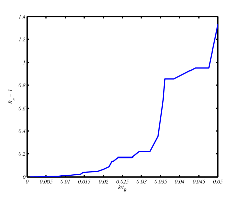
Figure 1: A “1%-Pareto” curve of error as a function of the size of $\hat{R}$

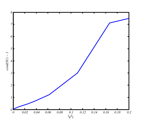
Figure 2: A 1%-Pareto curve of $\operatorname{\mathrm{cond}}(SU)-1$ as a function of the size of $\hat{S}$ relative to $\hat{R}$

Appendix A Deferred proofs

• Proof of Lemma 37:   Since by assumption $A$ has orthonormal columns, ${\|A(\tilde{X}-X^{*})\|}_{F}={\|A^{\top}A(\tilde{X}-X^{*})\|}_{F}$, so it suffices to bound the latter, or ${\|\beta\|}_{F}$ where $\beta\equiv A^{\top}A(\tilde{X}-X^{*})$. By Fact 35, we have

  $$A^{\top}S^{\top}S(A\tilde{X}-B)=0.$$ (12)

  To bound ${\|\beta\|}_{F}$, we bound ${\|A^{\top}S^{\top}SA\beta\|}_{F}$, and then show that this implies that ${\|\beta\|}_{F}$ is small. Using that $AA^{\top}A=A$ and (12), we have

  $$A^{\top}S^{\top}SA\beta =A^{\top}S^{\top}SAA^{\top}A(\tilde{X}-X^{*})$$

  $$=A^{\top}S^{\top}SA(\tilde{X}-X^{*})$$

  $$=A^{\top}S^{\top}SA(\tilde{X}-X^{*})+A^{\top}S^{\top}S(B-A\tilde{X})$$

  $$=A^{\top}S^{\top}S(B-AX^{*}).$$

  Using the hypothesis of the theorem,

  $${\|A^{\top}S^{\top}SA\beta\|}_{F}={\|A^{\top}S^{\top}S(B-AX^{*})\|}_{F}\leq\sqrt{\epsilon/r}{\|A\|}_{F}{\|B-AX^{*}\|}_{F}\leq\sqrt{\epsilon}{\|B-AX^{*}\|}_{F}.$$

  To show that this bound implies that ${\|\beta\|}_{F}$ is small, we use the subadditivity of ${\|\|}_{F}$ and the property of any conforming matrices $C$ and $D$, that ${\|CD\|}_{F}\leq{\|C\|}_{2}{\|D\|}_{F}$, to obtain

  $${\|\beta\|}_{F}\leq{\|A^{\top}S^{\top}SA\beta\|}_{F}+{\|A^{\top}S^{\top}SA\beta-\beta\|}_{F}\leq\sqrt{\epsilon}{\|B-AX^{*}\|}_{F}+{\|A^{\top}S^{\top}SA-I\|}_{2}{\|\beta\|}_{F}.$$

  By hypothesis, ${\|SAx\|}^{2}=(1\pm\epsilon_{0}){\|x\|}^{2}$ for all $x$, so that $A^{\top}S^{\top}SA-I$ has eigenvalues bounded in magnitude by $\epsilon_{0}^{2}$, which implies singular values with the same bound, so that ${\|A^{\top}S^{\top}SA-I\|}_{2}\leq\epsilon^{2}_{0}$. Thus ${\|\beta\|}_{F}\leq\sqrt{\epsilon}{\|B-AX^{*}\|}_{F}+\epsilon^{2}_{0}{\|\beta\|}_{F}$, or

  $${\|\beta\|}_{F}\leq\sqrt{\epsilon}{\|B-AX^{*}\|}_{F}/(1-\epsilon^{2}_{0})\leq 2\sqrt{\epsilon}{\|B-AX^{*}\|}_{F},$$

  since $\epsilon^{2}_{0}\leq 1/2$. This bounds ${\|\beta\|}_{F}$, and so proves the lemma.      

• Proof of Lemma 40:   Let $S=\Phi D$ with associated hash function $h:[n]\rightarrow[t]$. For $A_{i}$ denoting the $i$-th column of $A$, let $A_{i}(b)$ denote the column vector whose $\ell$-th coordinate is $0$ if $h(\ell)\neq b$, and whose $\ell$-th coordinate is $A_{\ell,i}$ if $h(\ell)=b$. We use the second moment method to bound $\|SA\|_{F}^{2}$. For the expectation,

  $${\bf E}_{D,h}[\|SA\|_{F}^{2}]=\sum_{i\in[d]}{\bf E}_{D,h}[\|SA_{i}\|_{2}^{2}]=\sum_{i\in[d]}\sum_{b\in[t]}{\bf E}_{D,h}[(\sum_{\ell\mid h(\ell)=b}A_{\ell,i}D_{\ell,\ell})^{2}]={\bf E}_{h}\left[\sum_{i\in[d]}\sum_{b\in[t]}\|A_{i}(b)\|_{2}^{2}\right]=\|A\|_{F}^{2}.$$ (13)

  For the second moment,

  $${\bf E}_{D,h}[\|SA\|_{F}^{4}]=\sum_{i\in[d]}{\bf E}_{D,h}[\|SA_{i}\|_{2}^{4}]+\sum_{i\neq j\in[d]}{\bf E}_{D,h}[\|SA_{i}\|_{2}^{2}\cdot\|SA_{j}\|_{2}^{2}].$$ (14)

  We handle the first term in (14) as follows:

  $${\bf E}_{D,h}[\|SA_{i}\|_{2}^{4}] = {\bf E}_{h}\left[\sum_{b,b^{\prime}\in[t]}{\bf E}_{D}[(SA_{i})_{b}^{2}\cdot(SA_{i})_{b^{\prime}}^{2}]\right]$$

  $$= {\bf E}_{h}\left[\sum_{b\in[t]}{\bf E}_{D}[(SA_{i})_{b}^{4}]+\sum_{b\neq b^{\prime}\in[t]}{\bf E}_{D}[(SA_{i})_{b}^{2}]\cdot{\bf E}_{D}[(SA_{i})_{b^{\prime}}^{2}]\right]$$

  $$= {\bf E}_{h}\left[\sum_{b\in[t]}{\bf E}_{D}[(\sum_{\ell\mid h(\ell)=b}A_{\ell,i}D_{\ell,\ell})^{4}]+\sum_{b\neq b^{\prime}\in[t]}{\bf E}_{D}[(\sum_{\ell\mid h(\ell)=b}A_{\ell,i}D_{\ell,\ell})^{2}]\cdot{\bf E}_{D}[(\sum_{\ell\mid h(\ell)=b^{\prime}}A_{\ell,i}D_{\ell,\ell})^{2}]\right]$$

  $$\leq {\bf E}_{h}\left[\sum_{b\in[t]}\left(\sum_{\ell\mid h(\ell)=b}A^{4}_{\ell,i}+{4\choose 2}\sum_{\ell<\ell^{\prime}\mid h(\ell)=h(\ell^{\prime})=b}A^{2}_{\ell,i}A^{2}_{\ell^{\prime},i}\right)+\sum_{b\neq b^{\prime}\in[t]}\|A_{i}(b)\|_{2}^{2}\cdot\|A_{i}(b^{\prime})\|_{2}^{2}\right]$$

  $$\leq {\bf E}_{h}\left[\|A_{i}\|_{4}^{4}\right]+\frac{6}{t}\|A_{i}\|_{2}^{4}+{\bf E}_{h}\left[\sum_{b\neq b^{\prime}\in[t]}\|A_{i}(b)\|_{2}^{2}\cdot\|A_{i}(b^{\prime})\|_{2}^{2}\right]$$

  $$\leq {\bf E}_{h}\left[\sum_{b\in[t]}\|A_{i}(b)\|_{2}^{4}\right]+\frac{6}{t}\|A_{i}\|_{2}^{4}+{\bf E}_{h}\left[\sum_{b\neq b^{\prime}\in[t]}\|A_{i}(b)\|_{2}^{2}\cdot\|A_{i}(b^{\prime})\|_{2}^{2}\right]$$

  $$\leq \frac{6}{t}\|A_{i}\|_{2}^{4}+\|A_{i}\|_{2}^{4}.$$

  For the second term in (14), for $i\neq j\in[d]$,

  $${\bf E}_{D,h}[\|SA_{i}\|_{2}^{2}\cdot\|SA_{j}\|_{2}^{2}] = {\bf E}_{D,h}\left[\sum_{b\in[t]}\left(\sum_{\ell\mid h(\ell)=b}A_{\ell,i}D_{\ell,\ell}\right)^{2}\left(\sum_{\ell^{\prime}\mid h(\ell^{\prime})=b}A_{\ell^{\prime},j}D_{\ell^{\prime},\ell^{\prime}}\right)^{2}\right]$$

  $$+{\bf E}_{D,h}\left[\sum_{b\neq b^{\prime}\in[t]}\left(\sum_{\ell\mid h(\ell)=b}A_{\ell,i}D_{\ell,\ell}\right)^{2}\left(\sum_{\ell^{\prime}\mid h(\ell^{\prime})=b^{\prime}}A_{\ell^{\prime},j}D_{\ell^{\prime},\ell^{\prime}}\right)^{2}\right]$$

  $$= {\bf E}_{h}\left[\sum_{b\in[t]}\left(\sum_{\ell,\ell^{\prime}\mid h(\ell)=h(\ell^{\prime})=b}A_{\ell,i}A_{\ell^{\prime},i}D_{\ell,\ell}D_{\ell^{\prime},\ell^{\prime}}\right)\left(\sum_{\ell,\ell^{\prime}\mid h(\ell)=h(\ell^{\prime})=b}A_{\ell,j}A_{\ell^{\prime},j}D_{\ell,\ell}D_{\ell^{\prime},\ell^{\prime}}\right)\right]$$

  $$+{\bf E}_{h}\left[\sum_{b\in[t]}\|A_{i}(b)\|_{2}^{2}\cdot\|A_{j}(b)\|_{2}^{2}+\sum_{b\neq b^{\prime}\in[t]}\|A_{i}(b)\|_{2}^{2}\cdot\|A_{j}(b^{\prime})\|_{2}^{2}\right]$$

  $$= \|A_{i}\|_{2}^{2}\cdot\|A_{j}\|_{2}^{2}+{\bf E}_{h}\left[\sum_{b\in[t]}4\sum_{\ell<\ell^{\prime}\mid h(\ell)=h(\ell^{\prime})=b}A_{\ell,i}A_{\ell^{\prime},i}A_{\ell,j}A_{\ell^{\prime},j}\right],$$

  where the constant $4$ arises because if we choose indices $\ell<\ell^{\prime}$ from $\left(\sum_{\ell,\ell^{\prime}\mid h(\ell)=h(\ell^{\prime})=b}A_{\ell,i}A_{\ell^{\prime},i}D_{\ell,\ell}D_{\ell^{\prime},\ell^{\prime}}\right)$ we need to choose the same $\ell$ and $\ell^{\prime}$ from $\left(\sum_{\ell,\ell^{\prime}\mid h(\ell)=h(\ell^{\prime})=b}A_{\ell,j}A_{\ell^{\prime},j}D_{\ell,\ell}D_{\ell^{\prime},\ell^{\prime}}\right)$ in order to have a non-zero expectation, and there are $4$ ways of doing this for distinct $\ell,\ell^{\prime}$. Continuing,

  $$\|A_{i}\|_{2}^{2}\cdot\|A_{j}\|_{2}^{2}+{\bf E}_{h}\left[\sum_{b\in[t]}4\sum_{\ell<\ell^{\prime}\mid h(\ell)=h(\ell^{\prime})=b}A_{\ell,i}A_{\ell^{\prime},i}A_{\ell,j}A_{\ell^{\prime},j}\right] \leq \|A_{i}\|_{2}^{2}\cdot\|A_{j}\|_{2}^{2}+{\bf E}_{h}\left[4\sum_{b\in[t]}\langle A_{i}(b),A_{j}(b)\rangle^{2}\right]$$

  $$\leq \|A_{i}\|_{2}^{2}\cdot\|A_{j}\|_{2}^{2}+{\bf E}_{h}\left[4\sum_{b\in[t]}\|A_{i}(b)\|_{2}^{2}\cdot\|A_{j}(b^{\prime})\|_{2}^{2}\right]$$

  $$= \|A_{i}\|_{2}^{2}\cdot\|A_{j}\|_{2}^{2}+\frac{4}{t}\sum_{\ell,\ell^{\prime}\in[n]}A_{\ell,i}^{2}A_{\ell,j}^{2}$$

  $$= \left(1+\frac{4}{t}\right)\|A_{i}\|_{2}^{2}\cdot\|A_{j}\|_{2}^{2}.$$

  Combining (13) with (14) and the bounds on the terms in (14) above,

  $${\bf Var}[\|SA\|_{F}^{2}] \leq \left(\sum_{i\in[d]}\frac{6}{t}\|A_{i}\|_{2}^{4}+\|A_{i}\|_{2}^{4}\right)+\sum_{i\neq j\in[d]}\left(1+\frac{4}{t}\right)\|A_{i}\|_{2}^{2}\cdot\|A_{j}\|_{2}^{2}-\|A\|_{F}^{2}$$

  $$\leq \frac{6}{t}\|A\|_{F}^{2}$$

  $$= \frac{6}{t}{\bf E}[\|SA\|_{F}^{2}].$$

  The lemma now follows by Chebyshev’s inequality, for appropriate $t=\Omega(\varepsilon^{-2})$.      

• Proof of Lemma 41:   Lemma 15 of [6] shows that ${\|SA\|}\leq(1+\varepsilon){\|A\|}$ with arbitrarily low failure probability, and the other direction follows from a similar argument. Briefly: the expectation of ${\|SA\|}^{2}$ is ${\|A\|}^{2}$, by construction, and Lemma 11 of [6] implies that with arbitrarily small failure probability, all rows of $SA$ will have squared norm at most $\beta\equiv\frac{\alpha}{t}{\|A\|}^{2}$, where $\alpha$ is a value in $O(\log n)$. Assuming that this bound holds, it follows from Hoeffding’s inequality that the probability that $|{\|SA\|}^{2}-{\|A\|}^{2}|\geq\varepsilon{\|A\|}^{2}$ is at most $2\exp(-2[\varepsilon{\|A\|}^{2}]^{2}/t\beta^{2})$, or $2\exp(-2\varepsilon^{2}t/\alpha^{2})$, so that $t=\Theta(\varepsilon^{-2}(\log n)^{2})$ suffices to make the failure probability at most $1/10$.      

• Proof of Lemma 49:   This is almost exactly the same as in [9], we simply adjust notation and parameters. Applying Theorem 28, we have that with probability at least $1-1/(100w)$, for all $x\in\mathbb{R}^{r}$, if we consider $y=Ax$ and write $y^{T}=[z_{1}^{T},z_{2}^{T},\ldots,z_{n/w}^{T}]$, then for all $i\in[n/w]$,

  $$\sqrt{\textstyle\frac{1}{2}}{\|z_{i}\|}_{2}\leq{\|Sz_{i}\|}_{2}\leq\sqrt{\textstyle\frac{3}{2}}{\|z_{i}\|}_{2}$$

  By relating the $2$-norm and the $p$-norm, for $1\leq p\leq 2$, we have

  $${\|Sz_{i}\|}_{p}\leq t^{1/p-1/2}{\|Sz_{i}\|}_{2}\leq t^{1/p-1/2}\sqrt{\textstyle\frac{3}{2}}{\|z_{i}\|}_{2}\leq t^{1/p-1/2}\sqrt{\textstyle\frac{3}{2}}{\|z_{i}\|}_{p},$$

  and similarly,

  $${\|Sz_{i}\|}_{p}\geq{\|Sz_{i}\|}_{2}\geq\sqrt{\textstyle\frac{1}{2}}{\|z_{i}\|}_{2}\geq\sqrt{\textstyle\frac{1}{2}}w^{1/2-1/p}{\|z_{i}\|}_{p}.$$

  If $p>2$, then

  $${\|Sz_{i}\|}_{p}\leq{\|Sz_{i}\|}_{2}\leq\sqrt{\textstyle\frac{3}{2}}{\|z_{i}\|}_{2}\leq\sqrt{\textstyle\frac{3}{2}}w^{1/2-1/p}{\|z_{i}\|}_{p},$$

  and similarly,

  $${\|Sz_{i}\|}_{p}\geq t^{1/p-1/2}{\|Sz_{i}\|}_{2}\geq t^{1/p-1/2}\sqrt{\textstyle\frac{1}{2}}{\|z_{i}\|}_{2}\geq t^{1/p-1/2}\sqrt{\textstyle\frac{1}{2}}{\|z_{i}\|}_{p}.$$

  Since ${\|Ax\|}_{p}^{p}={\|y\|}_{p}^{p}=\sum_{i}{\|z_{i}\|}^{p}$ and ${\|FAx\|}_{p}^{p}=\sum_{i}{\|Sz_{i}\|}_{p}^{p}$, for $p\in[1,2]$ we have with probability $1-1/(100w)$

  $$\sqrt{\textstyle\frac{1}{2}}w^{1/2-1/p}{\|Ax\|}_{p}\leq{\|FAx\|}_{p}\leq\sqrt{\textstyle\frac{3}{2}}t^{1/p-1/2}{\|Ax\|}_{p},$$

  and for $p\in[2,\infty)$ with probability $1-1/(100w)$

  $$\sqrt{\textstyle\frac{1}{2}}t^{1/p-1/2}{\|Ax\|}_{p}\leq{\|FAx\|}_{p}\leq\sqrt{\textstyle\frac{3}{2}}w^{1/2-1/p}{\|Ax\|}_{p}.$$

  In either case,

  $${\|Ax\|}_{p}\leq\gamma_{p}{\|FAx\|}_{p}\leq\sqrt{3}(tw)^{|1/p-1/2|}{\|Ax\|}_{p}.$$ (15)

Applying Theorem 48, we have, from the definition of a $(\alpha,\beta,p)$-well-conditioned basis, that

$$\|FAU\|_{p}\leq\alpha$$ (16)

and for all $x\in\mathbb{R}^{d}$,

$$\|x\|_{q}\leq\beta\|FAU\|_{p}.$$ (17)

Combining (15) and (16), we have that with probability at least $1-1/(100w)$,

$$\|AU/(r\gamma_{p})\|_{p}\leq\sum_{i}\|AU_{i}/r\gamma_{p}\|_{p}\leq\sum_{i}\|FAU_{i}/r\|_{p}\leq\alpha.$$

Combining (15) and (17), we have that with probability at least $1-1/(100w)$, for all $x\in\mathbb{R}^{r}$,

$$\|x\|_{q}\leq\beta\|FAUx\|_{p}\leq\beta\sqrt{3}r(tw)^{|1/p-1/2|}\|AU\frac{1}{r\gamma_{p}}x\|_{p}.$$

Hence $AU/(r\gamma_{p})$ is an $(\alpha,\beta\sqrt{3}r(tw)^{|1/p-1/2|},p)$-well-conditioned basis. The time to compute $FA$ is $O(\operatorname{\mathtt{nnz}}(A)\log n)$ by Theorem 28. Notice that $FA$ is an $nt/w\times n$ matrix, which is $O(n/r^{5})\times r$, and so the time to compute $U$ from $FA$ is $O((n/r^{5})r^{5}\log n)=O(\operatorname{\mathtt{nnz}}(A)\log n)$, since $\operatorname{\mathtt{nnz}}(A)\geq n$.

References

• [1] Dimitris Achlioptas, Amos Fiat, Anna R. Karlin, and Frank McSherry. Web search via hub synthesis. In FOCS, pages 500–509, 2001.
• [2] Dimitris Achlioptas and Frank McSherry. On spectral learning of mixtures of distributions. In COLT, pages 458–469, 2005.
• [3] Dimitris Achlioptas and Frank McSherry. Fast computation of low-rank matrix approximations. J. ACM, 54(2), 2007.
• [4] Sanjeev Arora, Elad Hazan, and Satyen Kale. A fast random sampling algorithm for sparsifying matrices. In APPROX-RANDOM, pages 272–279, 2006.
• [5] Yossi Azar, Amos Fiat, Anna R. Karlin, Frank McSherry, and Jared Saia. Spectral analysis of data. In STOC, pages 619–626, 2001.
• [6] C. Boutsidis and A. Gittens. Improved matrix algorithms via the Subsampled Randomized Hadamard Transform. ArXiv e-prints, March 2012.
• [7] Moses Charikar, Kevin Chen, and Martin Farach-Colton. Finding frequent items in data streams. Theor. Comput. Sci., 312(1):3–15, 2004.
• [8] Ho Yee Cheung, Tsz Chiu Kwok, and Lap Chi Lau. Fast matrix rank algorithms and applications. In STOC, pages 549–562, 2012.
• [9] K. Clarkson, P. Drineas, Malik Magdon-Ismail, M. Mahoney, Xiangrui Meng, and David P. Woodruff. The fast Cauchy transform and faster robust linear regression. In SODA, 2013.
• [10] Kenneth L. Clarkson and David P. Woodruff. Numerical linear algebra in the streaming model. In STOC, pages 205–214, 2009.
• [11] Anirban Dasgupta, Petros Drineas, Boulos Harb, Ravi Kumar, and Michael W. Mahoney. Sampling algorithms and coresets for $\ell_{p}$ regression. SIAM J. Comput., 38(5):2060–2078, 2009.
• [12] Anirban Dasgupta, Ravi Kumar, and Tamás Sarlós. A sparse Johnson-Lindenstrauss transform. In STOC, pages 341–350, 2010.
• [13] Amit Deshpande, Luis Rademacher, Santosh Vempala, and Grant Wang. Matrix approximation and projective clustering via volume sampling. In SODA, pages 1117–1126, 2006.
• [14] Amit Deshpande and Santosh Vempala. Adaptive sampling and fast low-rank matrix approximation. In APPROX-RANDOM, pages 292–303, 2006.
• [15] Petros Drineas, Alan M. Frieze, Ravi Kannan, Santosh Vempala, and V. Vinay. Clustering large graphs via the singular value decomposition. Machine Learning, 56(1-3):9–33, 2004.
• [16] Petros Drineas, Ravi Kannan, and Michael W. Mahoney. Fast Monte Carlo algorithms for matrices I: Approximating matrix multiplication. SIAM J. Comput., 36(1):132–157, 2006.
• [17] Petros Drineas, Ravi Kannan, and Michael W. Mahoney. Fast Monte Carlo algorithms for matrices II: Computing a low-rank approximation to a matrix. SIAM J. Comput., 36(1):158–183, 2006.
• [18] Petros Drineas, Ravi Kannan, and Michael W. Mahoney. Fast Monte Carlo algorithms for matrices III: Computing a compressed approximate matrix decomposition. SIAM J. Comput., 36(1):184–206, 2006.
• [19] Petros Drineas, Iordanis Kerenidis, and Prabhakar Raghavan. Competitive recommendation systems. In STOC, pages 82–90, 2002.
• [20] Petros Drineas, Malik Magdon-Ismail, Michael W. Mahoney, and David P. Woodruff. Fast approximation of matrix coherence and statistical leverage. CoRR, abs/1109.3843, 2011.
• [21] Petros Drineas, Michael Mahoney, Malik Magdon-Ismail, and David P. Woodruff. Fast approximation of matrix coherence and statistical leverage. In ICML, 2012.
• [22] Petros Drineas and Michael W. Mahoney. Approximating a Gram matrix for improved kernel-based learning. In COLT, pages 323–337, 2005.
• [23] Petros Drineas, Michael W. Mahoney, and S. Muthukrishnan. Sampling algorithms for $\ell_{2}$ regression and applications. In SODA, pages 1127–1136, 2006.
• [24] Petros Drineas, Michael W. Mahoney, and S. Muthukrishnan. Subspace sampling and relative-error matrix approximation: Column-based methods. In APPROX-RANDOM, pages 316–326, 2006.
• [25] Petros Drineas, Michael W. Mahoney, and S. Muthukrishnan. Subspace sampling and relative-error matrix approximation: Column-row-based methods. In ESA, pages 304–314, 2006.
• [26] Petros Drineas, Michael W. Mahoney, S. Muthukrishnan, and Tamás Sarlós. Faster least squares approximation. Numerische Mathematik, 117(2):217–249, 2011.
• [27] Alan M. Frieze, Ravi Kannan, and Santosh Vempala. Fast Monte-Carlo algorithms for finding low-rank approximations. J. ACM, 51(6):1025–1041, 2004.
• [28] Gene H. Golub and Charles F. van Loan. Matrix computations (3. ed.). Johns Hopkins University Press, 1996.
• [29] N. Halko, P.-G. Martinsson, and J. A. Tropp. Finding structure with randomness: Probabilistic algorithms for constructing approximate matrix decompositions. ArXiv e-prints, September 2009.
• [30] D.L. Hanson and F.T. Wright. A bound on tail probabilities for quadratic forms in independent random variables. The Annals of Mathematical Statistics, 42(3):1079–1083, 1971.
• [31] Daniel M. Kane and Jelani Nelson. A sparser Johnson-Lindenstrauss transform. CoRR, abs/1012.1577, 2010.
• [32] Daniel M. Kane and Jelani Nelson. Sparser Johnson-Lindenstrauss transforms. In SODA, pages 1195–1206, 2012.
• [33] Daniel M. Kane, Jelani Nelson, Ely Porat, and David P. Woodruff. Fast moment estimation in data streams in optimal space. In STOC, pages 745–754, 2011.
• [34] Ravindran Kannan, Hadi Salmasian, and Santosh Vempala. The spectral method for general mixture models. SIAM J. Comput., 38(3):1141–1156, 2008.
• [35] Jon M. Kleinberg. Authoritative sources in a hyperlinked environment. J. ACM, 46(5):604–632, 1999.
• [36] D.G. Luenberger and Y. Ye. Linear and nonlinear programming, volume 116. Springer Verlag, 2008.
• [37] Avner Magen and Anastasios Zouzias. Low rank matrix-valued Chernoff bounds and approximate matrix multiplication. In SODA, pages 1422–1436, 2011.
• [38] Frank McSherry. Spectral partitioning of random graphs. In FOCS, pages 529–537, 2001.
• [39] X. Meng and M. W. Mahoney. Low-distortion Subspace Embeddings in Input-sparsity Time and Applications to Robust Linear Regression. ArXiv e-prints, October 2012.
• [40] X. Meng, M. A. Saunders, and M. W. Mahoney. LSRN: A Parallel Iterative Solver for Strongly Over- or Under-Determined Systems. ArXiv e-prints, September 2011.
• [41] Gary L. Miller and Richard Peng. Iterative approaches to row sampling. CoRR, abs/1211.2713, 2012.
• [42] Jelani Nelson and Huy L. Nguyen. OSNAP: Faster numerical linear algebra algorithms via sparser subspace embeddings. CoRR, abs/1211.1002, 2012.
• [43] Jelani Nelson and David P. Woodruff. Fast Manhattan sketches in data streams. In PODS, pages 99–110, 2010.
• [44] Nam H. Nguyen, Thong T. Do, and Trac D. Tran. A fast and efficient algorithm for low-rank approximation of a matrix. In STOC, pages 215–224, 2009.
• [45] Christos H. Papadimitriou, Prabhakar Raghavan, Hisao Tamaki, and Santosh Vempala. Latent semantic indexing: A probabilistic analysis. J. Comput. Syst. Sci., 61(2):217–235, 2000.
• [46] Saurabh Paul, Christos Boutsidis, Malik Magdon-Ismail, and Petros Drineas. Random projections for support vector machines. CoRR, abs/1211.6085, 2012.
• [47] Benjamin Recht. A simpler approach to matrix completion. CoRR, abs/0910.0651, 2009.
• [48] M. Rudelson. Random vectors in the isotropic position. Journal of Functional Analysis, 164(1):60–72, 1999.
• [49] Mark Rudelson and Roman Vershynin. Sampling from large matrices: An approach through geometric functional analysis. J. ACM, 54(4), 2007.
• [50] Tamás Sarlós. Improved approximation algorithms for large matrices via random projections. In FOCS, pages 143–152, 2006.
• [51] Mikkel Thorup and Yin Zhang. Tabulation based 4-universal hashing with applications to second moment estimation. In SODA, pages 615–624, 2004.
• [52] Lloyd N. Trefethen and David Bau. Numerical linear algebra. SIAM, 1997.
• [53] Anastasios Zouzias. A matrix hyperbolic cosine algorithm and applications. CoRR, abs/1103.2793, 2011.
• [54] Anastasios Zouzias and Nikolaos M. Freris. Randomized extended Kaczmarz for solving least-squares. CoRR, abs/1205.5770, 2012.