Information content of weak lensing power spectrum and bispectrum: including the non-Gaussian error covariance matrix

Issha Kayo1, Masahiro Takada2 and Bhuvnesh Jain3
1 Department of Physics, Toho University, 2-2-1 Miyama, Funabashi, Chiba 274-8510, Japan
2 Kavli Institute for the Physics and Mathematics of the Universe (Kavli IPMU, WPI), The University of Tokyo, Chiba 277-8582, Japan
3 Department of Physics and Astronomy, University of Pennsylvania, Philadelphia, PA 19104, USA
E-mail: kayo@ph.sci.toho-u.ac.jpE-mail: masahiro.takada@ipmu.jpE-mail: bjain@physics.upenn.edu
Abstract

We address the amount of information in the non-Gaussian regime of weak lensing surveys by modelling all relevant covariances of the power spectra and bispectra, using 1000 ray-tracing simulation realizations for a ΛΛ\Lambda cold dark matter (ΛΛ\LambdaCDM) model and an analytical halo model. We develop a formalism to describe the covariance matrices of power spectra and bispectra of all triangle configurations. In addition to the known contributions which extend up to six-point correlation functions, we propose a new contribution ‘the halo sample variance (HSV)’ arising from the coupling of the lensing Fourier modes with large-scale mass fluctuations on scales comparable with the survey region via halo bias theory. We show that the model predictions are in good agreement with the simulation once we take the HSV into account. The HSV gives a dominant contribution to the covariance matrices at multipoles l103greater-than-or-similar-to𝑙superscript103l\ga 10^{3}, which arises from massive haloes with a mass of 1014Mgreater-than-or-similar-toabsentsuperscript1014subscript𝑀direct-product\ga 10^{14}M_{\odot} and at relatively low redshifts z0.4less-than-or-similar-to𝑧0.4z\la 0.4. Since such haloes are easily identified from a multi-colour imaging survey, the effect can be estimated from the data. By adding the bispectrum to the power spectrum, the total information content or the cumulative signal-to-noise ratio up to a certain maximum multipole lmaxsubscript𝑙maxl_{\rm max} of a few 103superscript10310^{3}, (S/N)lmaxsubscript𝑙max{}_{l_{\rm max}}, is improved by 20–50 per cent, which is equivalent to a factor of 1.4–2.3 larger survey area for the power spectrum measurement alone. However, it is still smaller than the case of a Gaussian field by a factor of 3 mostly due to the HSV. Thus bispectrum measurements are useful for cosmology, but using information from upcoming surveys requires that non-Gaussian covariances are carefully estimated.

keywords:
gravitational lensing: weak – cosmology: theory – large-scale structure of Universe.

1 Introduction

The accelerated expansion of the Universe is the most tantalizing problem in modern cosmology. Within Einstein’s gravity theory, general relativity, the cosmic acceleration can be explained by introducing dark energy, which acts as a repulsive, rather than attractive, force to expand the Universe. Alternatively, the cosmic acceleration may be a signature of the breakdown of general relativity on cosmological scales (see Jain & Khoury 2010, for a review). Many on-going and upcoming wide-area galaxy surveys aim at testing dark energy and modified gravity scenarios as the origin of cosmic acceleration; for example, the Canada–France–Hawaii Telescope (CFHT) Weak Lensing Survey 111http://www.cfhtlens.org/astronomers/content-suitable-astronomers, the Panoramic Survey Telescope & Rapid Response System (Pan-STARRS222http://pan-starrs.ifa.hawaii.edu), the VLT Survey Telescope (VST) Kilo-Degree Survey333http://www.astro-wise.org/projects/KIDS/, the Subaru Hyper Suprime-Cam Survey (Miyazaki et al. 2006)444http://www.naoj.org/Projects/HSC/index.html, the Dark Energy Survey (DES555http://www.darkenergysurvey.org), and in the next decade, the Large Synoptic Sky Survey (LSST666http://www.lsst.org), the European Space Agency (ESA) Euclid satellite mission777http://sci.esa.int/science-e/www/area/index.cfm?fareaid=102, and the NASA Wide-Field Infrared Survey Telescope (WFIRST) satellite mission. 888http://wfirst.gsfc.nasa.gov/

Among different cosmological probes, weak gravitational lensing or cosmic shear is recognized as one of the most promising methods for constraining the nature of dark energy, provided systematic errors are well under control (see Bartelmann & Schneider 2001; Schneider 2006; Hoekstra & Jain 2008, for reviews). The bending of light rays emitted from a distant galaxy due to the foreground mass distribution causes the image to be distorted. The distortion signal is too weak for us to measure in single galaxies, but we can use a sufficiently large number of galaxy images, available from wide-field survey, to detect the correlated shear signals existing in-between different galaxy images. Weak lensing is a unique method of measuring the total matter distribution including dark matter, free of galaxy bias uncertainty, and allows a direct comparison of the measurement with theory that is in most case about the statistical properties of the dark matter distribution. The theoretical predictions are obtained using N-body simulations (e.g. Springel et al. 2006) and/or analytical approaches (e.g. Bernardeau et al. 2002; Cooray & Sheth 2002). The cosmological weak lensing signal has been measured by several groups (e.g. Hamana et al. 2003; Hoekstra & Jain 2008; Schrabback et al. 2010, and also see references therein), and we are waiting for measurements with much higher statistical precision from upcoming surveys.

Most previous works on weak lensing, in theoretical and observational studies, have focused on the shear two-point correlation function or equivalently its Fourier transform, the power spectrum, as the statistics to quantify the lensing field. Although these statistics contain the full information when the field is a Gaussian random field as in the cosmic microwave background (CMB) field (Komatsu et al. 2011), it is not the case for the lensing field because non-linear clustering in structure formation causes a coupling between different Fourier modes, and the mass density field at redshifts relevant for lensing surveys is not Gaussian. In fact, various studies have shown that the information content carried by the power spectrum might be saturated at multipole scales of a few 103superscript10310^{3} [see Hamilton et al. (2006); Takahashi et al. (2009); Neyrinck et al. (2009) for the 3D mass density field, Sato et al. (2009) and Seo et al. (2011) for the lensing field, and Lee & Pen (2008) for the result from the actual data]. In particular, Sato et al. (2009) used 1000 ray-tracing simulation realizations for a ΛΛ\Lambda cold dark matter (ΛΛ\LambdaCDM) model to study the power spectrum covariance and the information content of the power spectrum. They found that the information content is reduced by a factor of 2 at multipoles l103similar-to-or-equals𝑙superscript103l\simeq 10^{3} compared to the Gaussian case for a survey with typical source redshift of zs1similar-to-or-equalssubscript𝑧𝑠1z_{s}\simeq 1. Further, they showed that large-scale mass density fluctuations of scales outside the simulation area contribute significantly to non-Gaussian terms of the covariance. They developed a formalism to describe the new non-Gaussian contribution by the number fluctuations of massive haloes based on halo bias theory, which we hereafter call the halo sample variance (HSV; also see Hu & Kravtsov 2003; Takada & Bridle 2007).

Some fundamental questions remain unresolved: how important and useful are the non-Gaussian signals in the lensing field for cosmology? Which statistical method to extract the non-Gaussian signals is most useful? Can we recover the Gaussian information content, which should have existed in the linear field or the primordial field, by combining the power spectrum and the non-Gaussian signals? For weak lensing, there is additional expectation that the non-Gaussian signals will be useful for cosmology, because the skewness, for example, has been shown complementary to the power spectrum in its dependence on cosmological parameters (Bernardeau et al. 1997; Jain & Seljak 1997; Hui 1999; Jain et al. 2000; White & Hu 2000; Hamana & Mellier 2001; Van Waerbeke et al. 2001; Cooray & Hu 2001b; Takada & Jain 2002, 2004; Dodelson & Zhang 2005; Kilbinger & Schneider 2005; Semboloni et al. 2008; Bergé et al. 2010; Munshi et al. 2011; Pires et al. 2012). The attempt to measure the non-Gaussian signals from actual data was also made by several groups (Bernardeau et al. 2002; Zhang et al. 2003; Jarvis et al. 2004), and the first significant detection was recently reported by Semboloni et al. (2011), showing an improvement in cosmological parameters compared to the two-point statistics alone.

In this paper, we study the lensing bispectrum, which contains the lowest-order non-Gaussianity of the weak lensing field and is a natural extension of the power spectrum. We consider all triangle configurations available from a given range of multipoles and their full covariance matrix including the non-Gaussian contributions up to six-point correlation functions as well as the HSV term, while only the Gaussian errors have been assumed in most previous work (Takada & Jain 2004; Martin et al. 2012). We use the 1000 simulation realizations to study the usefulness and complementarity of the lensing bispectrum compared to the power spectrum, and also develop an analytical formula to describe the bispectrum covariance for a given cosmology. In particular, we will show that the HSV gives a significant contribution to the bispectrum covariance at lgreater-than-or-similar-to𝑙absentl\ga a few 102superscript10210^{2}, and that the bispectrum does carry additional information to the power spectrum even in the presence of these significant correlations. Thus we will give a quantitative answer to the fundamental questions above.

This paper is organized as follows. After briefly reviewing the lensing power spectrum and bispectrum in Section 2, we develop a formulation to describe the bispectrum covariance in Section 3. In Section 4, we show the main results: we study the bispectrum covariance using both simulations and analytical model predictions. We quantify the information content of the lensing bispectrum by including contributions from all triangle configurations. Section 5 is devoted to discussion and conclusion.

2 Preliminaries: Lensing power spectrum and bispectrum

In the context of cosmological gravitational lensing, the convergence field is expressed as the weighted projection of the three-dimensional density fluctuation field between source and observer (see Bartelmann & Schneider 2001; Schneider 2006, for a thorough review)

κ(𝜽)=0χH𝑑χWGL(χ)δ[χ,χ𝜽],𝜅𝜽superscriptsubscript0subscript𝜒𝐻differential-d𝜒subscript𝑊GL𝜒𝛿𝜒𝜒𝜽\kappa(\mbox{\boldmath$\theta$})=\int_{0}^{\chi_{H}}\!\!d\chi W_{\rm GL}(\chi)\delta[\chi,\chi\mbox{\boldmath$\theta$}], (1)

where 𝜽𝜽\theta is the angular position on the sky, χ𝜒\chi is the comoving distance, and χHsubscript𝜒𝐻\chi_{H} is the distance to the Hubble horizon. We assume a flat geometry throughout this paper, and the radial distance χ𝜒\chi is equivalent to the comoving angular diameter distance. The comoving distance χ(a)𝜒𝑎\chi(a) from an observer at a=1𝑎1a=1 to a source at a𝑎a is expressed in terms of the Hubble expansion rate H(a)𝐻𝑎H(a) as χ(a)=a1𝑑a/[H(a)a2]𝜒𝑎subscriptsuperscript1𝑎differential-dsuperscript𝑎delimited-[]𝐻superscript𝑎superscript𝑎2\chi(a)=\int^{1}_{a}\!\!da^{\prime}/[H(a^{\prime})a^{\prime 2}]. For source galaxies at a single redshift, the lensing efficiency function WGL(χ)subscript𝑊GL𝜒W_{\rm GL}(\chi) is defined as

WGL(χ)32H02Ωm0a1χ(1χχs),subscript𝑊GL𝜒32superscriptsubscript𝐻02subscriptΩm0superscript𝑎1𝜒1𝜒subscript𝜒𝑠W_{\rm GL}(\chi)\equiv\frac{3}{2}H_{0}^{2}\Omega_{\rm m0}a^{-1}\chi\left(1-\frac{\chi}{\chi_{s}}\right), (2)

where χssubscript𝜒𝑠\chi_{s} is the distance to the source galaxies. See equation (4) in Takada & Jain (2009) for the lensing efficiency functions for tomographic redshift bins. Under the flat-sky approximation, the Fourier transform of the lensing field is defined as

κ(𝜽)=d2𝒍(2π)2κ~𝒍ei𝒍𝜽.𝜅𝜽superscript𝑑2𝒍superscript2𝜋2subscript~𝜅𝒍superscriptei𝒍𝜽\kappa(\mbox{\boldmath$\theta$})=\int\!\frac{d^{2}\mbox{\boldmath$l$}}{(2\pi)^{2}}\tilde{\kappa}_{\mbox{\boldmath$l$}}{\rm e}^{{\rm i}\mbox{\boldmath$l$}\cdot\mbox{\boldmath$\theta$}}. (3)

When the sky coverage of a survey is finite, we need to use the discrete Fourier decomposition, rather than the infinite-range Fourier decomposition (also see appendix in Takada & Bridle 2007, for details).

In this paper, we study the bispectrum of lensing field and the covariance of the bispectrum. The n𝑛n-point power spectra relevant for the bispectrum covariance are defined in terms of the ensemble averages of the convergence fields in Fourier space as

κ~𝒍1κ~𝒍2delimited-⟨⟩subscript~𝜅subscript𝒍1subscript~𝜅subscript𝒍2\displaystyle\langle{\tilde{\kappa}_{\mbox{\boldmath$l$}_{1}}\tilde{\kappa}_{\mbox{\boldmath$l$}_{2}}}\rangle \displaystyle\equiv (2π)2P(l1)δD2(𝒍1+𝒍2),superscript2𝜋2𝑃subscript𝑙1superscriptsubscript𝛿𝐷2subscript𝒍1subscript𝒍2\displaystyle(2\pi)^{2}P(l_{1})\delta_{D}^{2}(\mbox{\boldmath$l$}_{1}+\mbox{\boldmath$l$}_{2}), (4)
κ~𝒍1κ~𝒍2κ~𝒍3delimited-⟨⟩subscript~𝜅subscript𝒍1subscript~𝜅subscript𝒍2subscript~𝜅subscript𝒍3\displaystyle\langle{\tilde{\kappa}_{\mbox{\boldmath$l$}_{1}}\tilde{\kappa}_{\mbox{\boldmath$l$}_{2}}\tilde{\kappa}_{\mbox{\boldmath$l$}_{3}}}\rangle \displaystyle\equiv (2π)2B(𝒍1,𝒍2,𝒍3)δD2(𝒍1+𝒍2+𝒍3),superscript2𝜋2𝐵subscript𝒍1subscript𝒍2subscript𝒍3superscriptsubscript𝛿𝐷2subscript𝒍1subscript𝒍2subscript𝒍3\displaystyle(2\pi)^{2}B(\mbox{\boldmath$l$}_{1},\mbox{\boldmath$l$}_{2},\mbox{\boldmath$l$}_{3})\delta_{D}^{2}(\mbox{\boldmath$l$}_{1}+\mbox{\boldmath$l$}_{2}+\mbox{\boldmath$l$}_{3}), (5)
κ~𝒍1κ~𝒍2κ~𝒍3κ~𝒍4csubscriptdelimited-⟨⟩subscript~𝜅subscript𝒍1subscript~𝜅subscript𝒍2subscript~𝜅subscript𝒍3subscript~𝜅subscript𝒍4𝑐\displaystyle\langle{\tilde{\kappa}_{\mbox{\boldmath$l$}_{1}}\tilde{\kappa}_{\mbox{\boldmath$l$}_{2}}\tilde{\kappa}_{\mbox{\boldmath$l$}_{3}}\tilde{\kappa}_{\mbox{\boldmath$l$}_{4}}}\rangle_{c} \displaystyle\equiv (2π)2T(𝒍1,𝒍2,𝒍3,𝒍4)δD2(𝒍1+𝒍2+𝒍3),superscript2𝜋2𝑇subscript𝒍1subscript𝒍2subscript𝒍3subscript𝒍4superscriptsubscript𝛿𝐷2subscript𝒍1subscript𝒍2subscript𝒍3\displaystyle(2\pi)^{2}T(\mbox{\boldmath$l$}_{1},\mbox{\boldmath$l$}_{2},\mbox{\boldmath$l$}_{3},\mbox{\boldmath$l$}_{4})\delta_{D}^{2}(\mbox{\boldmath$l$}_{1}+\mbox{\boldmath$l$}_{2}+\mbox{\boldmath$l$}_{3}), (6)
κ~𝒍1κ~𝒍2κ~𝒍ncsubscriptdelimited-⟨⟩subscript~𝜅subscript𝒍1subscript~𝜅subscript𝒍2subscript~𝜅subscript𝒍𝑛𝑐\displaystyle\langle{\tilde{\kappa}_{\mbox{\boldmath$l$}_{1}}\tilde{\kappa}_{\mbox{\boldmath$l$}_{2}}\dots\tilde{\kappa}_{\mbox{\boldmath$l$}_{n}}}\rangle_{c} \displaystyle\equiv (2π)2Pn(𝒍1,𝒍2,,𝒍n)δD2(𝒍1+𝒍2++𝒍n)if n5,superscript2𝜋2subscript𝑃𝑛subscript𝒍1subscript𝒍2subscript𝒍𝑛superscriptsubscript𝛿𝐷2subscript𝒍1subscript𝒍2subscript𝒍𝑛if n5\displaystyle(2\pi)^{2}P_{n}(\mbox{\boldmath$l$}_{1},\mbox{\boldmath$l$}_{2},\dots,\mbox{\boldmath$l$}_{n})\delta_{D}^{2}(\mbox{\boldmath$l$}_{1}+\mbox{\boldmath$l$}_{2}+\cdots+\mbox{\boldmath$l$}_{n})\hskip 20.00003pt\mbox{if $n\geq 5$}, (7)

where δD2(𝒍)superscriptsubscript𝛿𝐷2𝒍\delta_{D}^{2}(\mbox{\boldmath$l$}) is the Dirac delta function; P𝑃P, B𝐵B and T𝑇T are the lensing power spectrum, bispectrum and trispectrum, respectively; Pnsubscript𝑃𝑛P_{n} is the n𝑛n-point power spectrum. For the bispectrum covariance, we need to include up to the six-point power spectra P6subscript𝑃6P_{6}. The higher-order correlation function than the bispectrum is the connected part of the n𝑛n-point function, which characterizes the non-Gaussianity of the lensing field and cannot be expressed in terms of products of the power spectrum (or any other lower-order correlation functions). Exchange symmetry of wavevectors, 𝒍i𝒍jsubscript𝒍𝑖subscript𝒍𝑗\mbox{\boldmath$l$}_{i}\leftrightarrow\mbox{\boldmath$l$}_{j}, reflects that the n𝑛n-point correlation functions are invariant under permutations of the arguments. The delta functions come from the parallel translation invariance for a statistically homogeneous field as is the convergence field.

The lensing power spectrum and bispectrum can be given as the weighted line-of-sight projection of the three-dimensional power spectrum and bispectrum of the underlying mass distribution. Employing Limber’s approximation (Limber 1954) and the flat-sky approximation, the lensing power spectrum and bispectrum are expressed as

P(l)𝑃𝑙\displaystyle P(l) =\displaystyle= 0χH𝑑χWGL2(χ)χ2Pδ(k=lχ;χ),superscriptsubscript0subscript𝜒𝐻differential-d𝜒subscriptsuperscript𝑊2GL𝜒superscript𝜒2subscript𝑃𝛿𝑘𝑙𝜒𝜒\displaystyle\int_{0}^{\chi_{H}}\!d\chi W^{2}_{\rm GL}(\chi)\chi^{-2}P_{\delta}\left(k=\frac{l}{\chi};\chi\right), (8)
B(𝒍1,𝒍2,𝒍3)𝐵subscript𝒍1subscript𝒍2subscript𝒍3\displaystyle B(\mbox{\boldmath$l$}_{1},\mbox{\boldmath$l$}_{2},\mbox{\boldmath$l$}_{3}) =\displaystyle= 0χH𝑑χWGL3(χ)χ4Bδ(𝒌1,𝒌2,𝒌3;χ)|𝒌i=𝒍i/χ,evaluated-atsubscriptsuperscriptsubscript𝜒𝐻0differential-d𝜒superscriptsubscript𝑊GL3𝜒superscript𝜒4subscript𝐵𝛿subscript𝒌1subscript𝒌2subscript𝒌3𝜒subscript𝒌𝑖subscript𝒍𝑖𝜒\displaystyle\int^{\chi_{H}}_{0}\!d\chi W_{\rm GL}^{3}(\chi)\chi^{-4}\left.B_{\delta}(\mbox{\boldmath$k$}_{1},\mbox{\boldmath$k$}_{2},\mbox{\boldmath$k$}_{3};\chi)\right|_{\mbox{\boldmath$k$}_{i}=\mbox{\boldmath$l$}_{i}/\chi}, (9)

where Pδsubscript𝑃𝛿P_{\delta} and Bδsubscript𝐵𝛿B_{\delta} are the power spectrum and bispectrum of the mass distribution at each redshift χ(=χ(z))annotated𝜒absent𝜒𝑧\chi(=\chi(z)). Thus once the n𝑛n-point spectra of the mass density field are given for a given cosmological model, we can compute the n𝑛n-point spectra of the lensing field. The above equations also mean that statistical properties of the lensing field arise from those of the mass density field, since the prefactors such as the WGL(χ)subscript𝑊GL𝜒W_{\rm GL}(\chi) are pure geometrical quantities, not statistical variables.

The power spectrum measurement for an actual survey is affected by the intrinsic shape noise due to a finite sampling of source galaxy shapes:

Pobs(l)=P(l)+σϵ2n¯g,superscript𝑃obs𝑙𝑃𝑙superscriptsubscript𝜎italic-ϵ2subscript¯𝑛𝑔P^{\rm obs}(l)=P(l)+\frac{\sigma_{\epsilon}^{2}}{\bar{n}_{g}}, (10)

where σϵsubscript𝜎italic-ϵ\sigma_{\epsilon} is the rms of intrinsic ellipticities per component, and n¯gsubscript¯𝑛𝑔\bar{n}_{g} is the mean number density of source galaxies per unit steradian. In the following, we will often omit the notation obs to refer Pobs(l)superscript𝑃obs𝑙P^{\rm obs}(l) for notational simplicity. Throughout this paper we assume that the orientation of intrinsic galaxy shape is random and the shapes of different galaxies are uncorrelated; the shape noise is a Gaussian random field. The bispectrum is a measure of the non-Gaussianity, so is not affected by the shape noise.

3 Lensing Covariance

The covariances of the lensing spectrum and bispectrum describe a measurement accuracy of the spectra for a given survey. There are several sources of the measurement errors: the shot noise arising due to a finite sampling of galaxy shapes and the sample variance arising due to a finite survey area. If the lensing field is Gaussian, the different Fourier modes with 𝒍𝒍𝒍superscript𝒍\mbox{\boldmath$l$}\neq\mbox{\boldmath$l$}^{\prime} are independent, and therefore the sample variance is determined by the number of independent Fourier modes for a given multipole bin l𝑙l that are available from the survey, yielding a simple formula of the sample variance contribution (e.g. Knox 1995). However, this is not the case for the lensing field, because the lensing field is highly non-Gaussian at scales of interest (Takada & Jain 2004, 2009; Sato et al. 2009), and the different Fourier modes correlate with each other. In the following, we discuss theory for the lensing covariance matrices.

3.1 Power spectrum covariance

The power spectrum covariance has been well studied by previous works (Scoccimarro et al. 1999; Cooray & Hu 2001a; Takada & Bridle 2007; Takada & Jain 2009; Sato et al. 2009). In particular, Sato et al. (2009) derived an expression of the power spectrum covariance including a new contribution from the mass density fluctuations at larger scales than the survey area, and showed that the formula well reproduces their ray-tracing simulation results. According to this work, the power spectrum covariance is given as

Cov[P(li),P(lj)]Cov𝑃subscript𝑙𝑖𝑃subscript𝑙𝑗\displaystyle{\rm Cov}[P(l_{i}),P(l_{j})] =\displaystyle= 2δliljKNpairs(l)[P(li)+σϵ2n¯g]2+1Ωs|𝒍|lid2𝒍A(li)|𝒍|ljd2𝒍A(lj)T(𝒍,𝒍,𝒍,𝒍)+CovHSVPP(li,lj;Ωs),2subscriptsuperscript𝛿𝐾subscript𝑙𝑖subscript𝑙𝑗subscript𝑁pairs𝑙superscriptdelimited-[]𝑃subscript𝑙𝑖superscriptsubscript𝜎italic-ϵ2subscript¯𝑛𝑔21subscriptΩssubscript𝒍subscript𝑙𝑖superscript𝑑2𝒍𝐴subscript𝑙𝑖subscriptsuperscript𝒍subscript𝑙𝑗superscript𝑑2superscript𝒍𝐴subscript𝑙𝑗𝑇𝒍𝒍superscript𝒍superscript𝒍subscriptsuperscriptCov𝑃𝑃HSVsubscript𝑙𝑖subscript𝑙𝑗subscriptΩs\displaystyle\frac{2\delta^{K}_{l_{i}l_{j}}}{N_{\rm pairs}(l)}\left[P(l_{i})+\frac{\sigma_{\epsilon}^{2}}{\bar{n}_{g}}\right]^{2}+\frac{1}{\Omega_{\rm s}}\int_{\left|\mbox{\boldmath$l$}\right|\in l_{i}}\!\frac{d^{2}\mbox{\boldmath$l$}}{A(l_{i})}\int_{\left|\mbox{\boldmath$l$}^{\prime}\right|\in l_{j}}\!\frac{d^{2}\mbox{\boldmath$l$}^{\prime}}{A(l_{j})}T(\mbox{\boldmath$l$},-\mbox{\boldmath$l$},\mbox{\boldmath$l$}^{\prime},-\mbox{\boldmath$l$}^{\prime})+{\rm Cov}^{PP}_{\rm HSV}(l_{i},l_{j};\Omega_{\rm s}), (11)

where δliljKsubscriptsuperscript𝛿𝐾subscript𝑙𝑖subscript𝑙𝑗\delta^{K}_{l_{i}l_{j}} is the Kronecker delta, δliljK=1subscriptsuperscript𝛿𝐾subscript𝑙𝑖subscript𝑙𝑗1\delta^{K}_{l_{i}l_{j}}=1 if li=ljsubscript𝑙𝑖subscript𝑙𝑗l_{i}=l_{j} within the bin width and otherwise δliljK=0subscriptsuperscript𝛿𝐾subscript𝑙𝑖subscript𝑙𝑗0\delta^{K}_{l_{i}l_{j}}=0; ΩssubscriptΩs\Omega_{\rm s} is the survey area in units of steradian; A(li)𝐴subscript𝑙𝑖A(l_{i}) is the area of the above integration in Fourier space, given as As(li)|𝒍|lid2𝒍subscript𝐴𝑠subscript𝑙𝑖subscript𝒍subscript𝑙𝑖superscript𝑑2𝒍A_{s}(l_{i})\equiv\int_{\left|\mbox{\boldmath$l$}\right|\in l_{i}}d^{2}\mbox{\boldmath$l$}, where the integration range is confined to the wavevectors satisfying the condition liΔl/2|𝒍|li+Δl/2subscript𝑙𝑖Δ𝑙2𝒍subscript𝑙𝑖Δ𝑙2l_{i}-\Delta l/2\leq|\mbox{\boldmath$l$}|\leq l_{i}+\Delta l/2 (ΔlΔ𝑙\Delta l is the bin width around the i𝑖ith bin, lisubscript𝑙𝑖l_{i}); the third term CovHSVsubscriptCovHSV{\rm Cov}_{\rm HSV} is the new contribution which we call the halo sample variance (HSV) contribution (see below). The quantity Npairs(li)subscript𝑁pairssubscript𝑙𝑖N_{\rm pairs}(l_{i}) is the number of independent pairs of two vectors 𝒍𝒍l and 𝒍𝒍-\mbox{\boldmath$l$} in Fourier space, where the vector 𝒍𝒍l has the length lisubscript𝑙𝑖l_{i} within the bin width and “independent” here means different pairs discriminated by the fundamental Fourier mode of a given survey, lf2π/Θssimilar-to-or-equalssubscript𝑙𝑓2𝜋subscriptΘsl_{f}\simeq 2\pi/\Theta_{\rm s} (ΘssubscriptΘs\Theta_{\rm s} is the angular scale of the survey area). At the limit lilfmuch-greater-thansubscript𝑙𝑖subscript𝑙𝑓l_{i}\gg l_{f}, A(li)2πliΔlsimilar-to-or-equals𝐴subscript𝑙𝑖2𝜋subscript𝑙𝑖Δ𝑙A(l_{i})\simeq 2\pi l_{i}\Delta l and the number of independent Fourier modes is given as

Npairs(li)2πliΔl(2π/Θs)2=ΩsliΔl2π=2fskyliΔl,similar-to-or-equalssubscript𝑁pairssubscript𝑙𝑖2𝜋subscript𝑙𝑖Δ𝑙superscript2𝜋subscriptΘs2subscriptΩssubscript𝑙𝑖Δ𝑙2𝜋2subscript𝑓skysubscript𝑙𝑖Δ𝑙N_{\rm pairs}(l_{i})\simeq\frac{2\pi l_{i}\Delta l}{(2\pi/\Theta_{\rm s})^{2}}=\frac{\Omega_{\rm s}l_{i}\Delta l}{2\pi}=2f_{\rm sky}l_{i}\Delta l, (12)

where fskysubscript𝑓skyf_{\rm sky} is the sky fraction defined as fskyΩs/4πsubscript𝑓skysubscriptΩs4𝜋f_{\rm sky}\equiv\Omega_{\rm s}/4\pi. See Takada & Bridle (2007) for a pedagogical derivation of the power spectrum covariance based on the discrete Fourier decomposition formulation (except for the third term CovHSVPPsubscriptsuperscriptCov𝑃𝑃HSV{\rm Cov}^{PP}_{\rm HSV}). In equation (11), we ignored effects of non-trivial survey geometry for simplicity.

The first and second terms on the r.h.s. of equation (11) are the standard covariance terms studied in most previous works. The first term describes the Gaussian covariance term that vanishes when liljsubscript𝑙𝑖subscript𝑙𝑗l_{i}\neq l_{j}, i.e. no correlation between different multipole bins. The second term gives a non-Gaussian term arising from the lensing trispectrum (four-point correlation function), which describes the mode coupling between different multipole bins. Both terms scale with survey area as 1/Ωs1subscriptΩs1/\Omega_{\rm s}; the amplitudes decrease with increasing the survey area. It should also be noted that the Gaussian term depends on the multipole bin width, while the non-Gaussian terms do not; a larger bin width relatively reduces the Gaussian term contribution at the multipole bin.

The third term of equation (11) arises from the mode coupling of the Fourier mode of our interest, lisubscript𝑙𝑖l_{i}, with large-scale modes of scales comparable with or even outside the survey region. Such large-scale modes cannot be seen by an observer, but affect the power spectrum estimation. If the entire survey region happens to be in an overdense/underdense region, which is caused by the large-scale mass density fluctuations, the number of massive haloes becomes larger/smaller than the ensemble average according to the halo bias theory (Mo & White 1996; Sheth et al. 2001). Thus the number of massive haloes found in a finite survey volume correlates with the mass density fluctuations of scales comparable with or larger than the survey field (Hu & Kravtsov 2003). To be more explicit, the number fluctuations of haloes in a mass M𝑀M and in the redshift slice centred at z𝑧z are given as

δN(M)=b(M)d2VdzdΩΩsΔzdndMδ¯m(Θs;z),𝛿𝑁𝑀𝑏𝑀superscript𝑑2𝑉𝑑𝑧𝑑ΩsubscriptΩsΔ𝑧𝑑𝑛𝑑𝑀subscript¯𝛿𝑚subscriptΘs𝑧\delta N(M)=b(M)\frac{d^{2}V}{dzd\Omega}\Omega_{\rm s}\Delta z\frac{dn}{dM}\bar{\delta}_{m}(\Theta_{\rm s};z), (13)

where d2V/dzdΩsuperscript𝑑2𝑉𝑑𝑧𝑑Ωd^{2}V/dzd\Omega is the comoving volume per unit redshift interval and per unit solid angle, d2V/dzdΩ=χ2superscript𝑑2𝑉𝑑𝑧𝑑Ωsuperscript𝜒2d^{2}V/dzd\Omega=\chi^{2} for a flat universe; dn/dM𝑑𝑛𝑑𝑀dn/dM is the ensemble-averaged mass function of haloes in the mass range [M,M+dM]𝑀𝑀𝑑𝑀[M,M+dM]; b(M)𝑏𝑀b(M) is the halo bias parameter; δm(Θs)subscript𝛿𝑚subscriptΘ𝑠\delta_{m}(\Theta_{s}) is the mass density fluctuation averaged within the survey volume in the redshift slice which has area ΩssubscriptΩs\Omega_{\rm s} and the redshift width ΔzΔ𝑧\Delta z. The lensing power spectrum amplitudes at small angular scales are sensitive to the number of massive haloes in the survey region and then correlates with the number fluctuations, which results in the HSV. Note that the ensemble average of the power spectrum is not affected by the large-scale mode due to the fact δ¯m(Θs)=0delimited-⟨⟩subscript¯𝛿𝑚subscriptΘs0\left\langle{\bar{\delta}_{m}(\Theta_{\rm s})}\right\rangle=0. At the limit of li,lj1much-greater-thansubscript𝑙𝑖subscript𝑙𝑗1l_{i},l_{j}\gg 1, the HSV contribution is given as

CovHSVPP(li,lj;Ωs)=0χs𝑑χ(d2VdΩdχ)2[𝑑MdndMb(M)|κ~li|2][𝑑MdndMb(M)|κ~lj|2][0kdk2πPmL(k)|W~(kχΘs)|2],subscriptsuperscriptCov𝑃𝑃HSVsubscript𝑙𝑖subscript𝑙𝑗subscriptΩssubscriptsuperscriptsubscript𝜒𝑠0differential-d𝜒superscriptsuperscript𝑑2𝑉𝑑Ω𝑑𝜒2delimited-[]differential-d𝑀𝑑𝑛𝑑𝑀𝑏𝑀superscriptsubscript~𝜅subscript𝑙𝑖2delimited-[]differential-dsuperscript𝑀𝑑𝑛𝑑superscript𝑀𝑏superscript𝑀superscriptsubscript~𝜅subscript𝑙𝑗2delimited-[]superscriptsubscript0𝑘𝑑𝑘2𝜋superscriptsubscript𝑃𝑚𝐿𝑘superscript~𝑊𝑘𝜒subscriptΘs2{\rm Cov}^{PP}_{\rm HSV}(l_{i},l_{j};\Omega_{\rm s})=\int^{\chi_{s}}_{0}\!\!d\chi\left(\frac{d^{2}V}{d\Omega d\chi}\right)^{2}\left[\int\!\!dM\frac{dn}{dM}b(M)\left|\tilde{\kappa}_{l_{i}}\right|^{2}\right]\left[\int\!\!dM^{\prime}\frac{dn}{dM^{\prime}}b(M^{\prime})\left|\tilde{\kappa}_{l_{j}}\right|^{2}\right]\left[\int_{0}^{\infty}\!\!\frac{kdk}{2\pi}P_{m}^{L}(k)\left|\tilde{W}(k\chi\Theta_{\rm s})\right|^{2}\right], (14)

where W~(l)~𝑊𝑙\tilde{W}(l) is the Fourier transform of the survey window function; PmLsuperscriptsubscript𝑃𝑚𝐿P_{m}^{L} is the linear mass power spectrum; κ~l(χ)subscript~𝜅𝑙𝜒\tilde{\kappa}_{l}(\chi) is the Fourier transform of the convergence field for which we assume a Navarro-Frenk-White (NFW) halo (Navarro et al. 1997) (see equation 28 in Oguri & Takada 2011 or section 3.2 in Takada & Jain 2003b for the expression of κ~lsubscript~𝜅𝑙\tilde{\kappa}_{l}). For notational simplicity, we omit to denote the redshift dependence of dn/dM𝑑𝑛𝑑𝑀dn/dM, b(M)𝑏𝑀b(M) and κ~lsubscript~𝜅𝑙\tilde{\kappa}_{l}. In this paper, we simply consider the window function given by W~(x)=2J1(x)/x~𝑊𝑥2subscript𝐽1𝑥𝑥\tilde{W}(x)=2J_{1}(x)/x, which corresponds to a circle-shaped survey geometry with a radius of ΘssubscriptΘs\Theta_{\rm s}. For the halo model ingredients [dn/dM,b(M)𝑑𝑛𝑑𝑀𝑏𝑀dn/dM,b(M) and the NFW profile], we will throughout this paper employ the same models as used in Takada & Jain (2009). Roughly speaking, the HSV term can be expressed as CovHSVPPP1h(li)P1h(lj)σm2(Ωs)similar-tosuperscriptsubscriptCovHSV𝑃𝑃subscript𝑃1subscript𝑙𝑖subscript𝑃1subscript𝑙𝑗subscriptsuperscript𝜎2𝑚subscriptΩs{\rm Cov}_{\rm HSV}^{PP}\sim P_{1h}(l_{i})P_{1h}(l_{j})\sigma^{2}_{m}(\Omega_{\rm s}), where P1hsubscript𝑃1P_{1h} is the one-halo term of the lensing power spectrum and σm(Ωs)subscript𝜎𝑚subscriptΩs\sigma_{m}(\Omega_{\rm s}) is the rms of the projected linear mass density fluctuations smoothed with the angular scale of the survey area. As implied from the above equation, the HSV affects the band powers of different multipoles in the same way, and does not change the shape of the power spectrum. This HSV term cannot be realized as long as the discrete Fourier decomposition is used for deriving the power spectrum covariance, because the large-scale modes outside the survey region cannot be described by Fourier modes confined inside the survey region.

Another important feature is that the HSV contribution depends on the survey area via the integration of the linear mass power spectrum, k𝑑kPmL(k)|W~(kχΘs)|2𝑘differential-d𝑘superscriptsubscript𝑃𝑚𝐿𝑘superscript~𝑊𝑘𝜒subscriptΘs2\int\!kdkP_{m}^{L}(k)\left|\tilde{W}(k\chi\Theta_{\rm s})\right|^{2} unlike the other terms which scale as 1/Ωs1subscriptΩs1/\Omega_{\rm s}. For a power-law linear power spectrum, PmL(k)knproportional-tosubscriptsuperscript𝑃𝐿𝑚𝑘superscript𝑘𝑛P^{L}_{m}(k)\propto k^{n}, the HSV term is found to scale as CovHSVPP1/(Ωs)1+n/2proportional-tosubscriptsuperscriptCov𝑃𝑃HSV1superscriptsubscriptΩs1𝑛2{\rm Cov}^{PP}_{\rm HSV}\propto 1/(\Omega_{\rm s})^{1+n/2}. Hence, for n<0𝑛0n<0, which is indeed the case at kkeq𝑘subscript𝑘eqk\geq k_{\rm eq} (keqsubscript𝑘eqk_{\rm eq} is the wavenumber of the matter-radiation equality), the HSV amplitude decreases more slowly with increasing area coverage than other terms. On the other hand, when n>0𝑛0n>0 or kkeq𝑘subscript𝑘eqk\leq k_{\rm eq}, the HSV term decreases more quickly. Thus the HSV term depends on the survey area in a non-trivial way, and we will study the relative importance of the HSV term for different survey areas.

There are even other sources of non-Gaussian errors arising from a correlation of the lensing field in the weakly non-linear regime with the mass density fluctuations of scales comparable with or larger than the survey area. This contribution can be formulated based on the perturbation theory of structure formation, which is valid for the mass density field in the weakly non-linear regime. Rimes & Hamilton (2005) first studied this effect for the 3D mass power spectrum, and named this new contribution the beat-coupling mode (also see Hamilton et al. 2006; Sefusatti et al. 2006; Takahashi et al. 2009). Furthermore, de Putter et al. (2012) recently pointed out that the large-scale density fluctuations cause an apparent modulation in the mean density estimated from a finite survey region, and add an additional negative contribution to the covariance. This term was shown to have a similar amplitude to the beat-coupling mode. These large-scale mode contribution, which is relevant for the weakly non-linear regime, differs from the HSV effect, and Takada & Jain (2009) showed that the contribution to the lensing power spectrum covariance is negligible compared to the non-Gaussian errors arising from the four-point function (the second term in equation 11) at multipoles of lgreater-than-or-similar-to𝑙absentl\ga a few 102superscript10210^{2}. Hence, in this paper, we ignore the non-Gaussian errors arising from the mode-coupling in the weakly non-linear regime for simplicity.

3.2 Bispectrum covariance

As we discussed above, the lensing bispectrum is given as a function of triangle configurations. An estimator of the lensing bispectrum from the finite-area lensing survey can be found, by extending the method developed in Takada & Bridle (2007) (see Appendix A for the details), as

B^(l1,l2,l3)=1ΩsNtrip(l1,l2,l3)𝒒iκ~𝒒1κ~𝒒2κ~𝒒3Δ𝒒123(l1,l2,l3),^𝐵subscript𝑙1subscript𝑙2subscript𝑙31subscriptΩssubscript𝑁tripsubscript𝑙1subscript𝑙2subscript𝑙3subscriptsubscript𝒒𝑖subscript~𝜅subscript𝒒1subscript~𝜅subscript𝒒2subscript~𝜅subscript𝒒3subscriptΔsubscript𝒒123subscript𝑙1subscript𝑙2subscript𝑙3\hat{B}({l}_{1},{l}_{2},{l}_{3})=\frac{1}{\Omega_{\rm s}N_{\rm trip}(l_{1},l_{2},l_{3})}\sum_{\mbox{\boldmath$q$}_{i}}\tilde{\kappa}_{\mbox{\boldmath$q$}_{1}}\tilde{\kappa}_{\mbox{\boldmath$q$}_{2}}\tilde{\kappa}_{\mbox{\boldmath$q$}_{3}}\Delta_{\mbox{\boldmath$q$}_{123}}(l_{1},l_{2},l_{3}), (15)

where 𝒒123𝒒1+𝒒2+𝒒3subscript𝒒123subscript𝒒1subscript𝒒2subscript𝒒3\mbox{\boldmath$q$}_{123}\equiv\mbox{\boldmath$q$}_{1}+\mbox{\boldmath$q$}_{2}+\mbox{\boldmath$q$}_{3} and the summation runs over all the pixels of 𝒒1subscript𝒒1\mbox{\boldmath$q$}_{1}, 𝒒2subscript𝒒2\mbox{\boldmath$q$}_{2} and 𝒒3subscript𝒒3\mbox{\boldmath$q$}_{3}. The function Δ𝒒123subscriptΔsubscript𝒒123\Delta_{\mbox{\boldmath$q$}_{123}} denotes the selection function which is unity if each vector has a target length of liΔli/2qili+Δli/2subscript𝑙𝑖Δsubscript𝑙𝑖2subscript𝑞𝑖subscript𝑙𝑖Δsubscript𝑙𝑖2l_{i}-\Delta l_{i}/2\leq q_{i}\leq l_{i}+\Delta l_{i}/2 (i=1,2,3𝑖123i=1,2,3) and the three vectors form the triangle configuration in Fourier space, 𝒒123=𝟎subscript𝒒1230\mbox{\boldmath$q$}_{123}=\mbox{\boldmath$0$}; otherwise Δ𝒒123(l1,l2,l3)=0subscriptΔsubscript𝒒123subscript𝑙1subscript𝑙2subscript𝑙30\Delta_{\mbox{\boldmath$q$}_{123}}(l_{1},l_{2},l_{3})=0. The prefactor 1/Ωs1subscriptΩs1/\Omega_{\rm s} is from our definition of the discrete Fourier decomposition (see Takada & Bridle 2007). The quantity Ntripsubscript𝑁tripN_{\rm trip} is the number of the triplets in Fourier space that form a given triangle configuration specified by three side lengths l1,l2,l3subscript𝑙1subscript𝑙2subscript𝑙3l_{1},l_{2},l_{3} with the bin widths. This is calculated from the selection function as Ntrip=𝒒iΔ𝒒123(l1,l2,l3)subscript𝑁tripsubscriptsubscript𝒒𝑖subscriptΔsubscript𝒒123subscript𝑙1subscript𝑙2subscript𝑙3N_{\rm trip}=\sum_{\mbox{\boldmath$q$}_{i}}\Delta_{\mbox{\boldmath$q$}_{123}}(l_{1},l_{2},l_{3}). As described in Joachimi et al. (2009) and Appendix A, for the limit of large multipole bins, l1,l2,l3lfmuch-greater-thansubscript𝑙1subscript𝑙2subscript𝑙3subscript𝑙𝑓l_{1},l_{2},l_{3}\gg l_{f}, we can analytically estimate Ntripsubscript𝑁tripN_{\rm trip} as

Ntrip(l1,l2,l3)subscript𝑁tripsubscript𝑙1subscript𝑙2subscript𝑙3\displaystyle N_{\rm trip}(l_{1},l_{2},l_{3}) \displaystyle\equiv 𝒒i;qiliΔ𝒒123Ωs2l1l2l3Δl1Δl2Δl32π32l12l22+2l12l32+2l22l32l14l24l34,similar-to-or-equalssubscriptsubscript𝒒𝑖subscript𝑞𝑖subscript𝑙𝑖subscriptΔsubscript𝒒123subscriptsuperscriptΩ2ssubscript𝑙1subscript𝑙2subscript𝑙3Δsubscript𝑙1Δsubscript𝑙2Δsubscript𝑙32superscript𝜋32superscriptsubscript𝑙12superscriptsubscript𝑙222superscriptsubscript𝑙12superscriptsubscript𝑙322superscriptsubscript𝑙22superscriptsubscript𝑙32superscriptsubscript𝑙14superscriptsubscript𝑙24superscriptsubscript𝑙34\displaystyle\sum_{\mbox{\boldmath$q$}_{i};q_{i}\in l_{i}}\Delta_{\mbox{\boldmath$q$}_{123}}\simeq\frac{\Omega^{2}_{\rm s}l_{1}l_{2}l_{3}\Delta l_{1}\Delta l_{2}\Delta l_{3}}{2\pi^{3}\sqrt{2l_{1}^{2}l_{2}^{2}+2l_{1}^{2}l_{3}^{2}+2l_{2}^{2}l_{3}^{2}-l_{1}^{4}-l_{2}^{4}-l_{3}^{4}}}, (16)

where ΔliΔsubscript𝑙𝑖\Delta l_{i} is the bin width of the i𝑖ith side length. For the small-angle scales li1much-greater-thansubscript𝑙𝑖1l_{i}\gg 1 (flat-sky approximation limit) we are interested in, this equation gives a good approximation to the Wigner- 3j𝑗j symbols which appears in the bispectrum covariance derived under the full-sky approach (see equation 16 in Takada & Jain 2004).

The bispectrum covariance can be similarly defined as

Cov[B(𝒍1,𝒍2,𝒍3),B(𝒍1,𝒍2,𝒍3)]Cov𝐵subscript𝒍1subscript𝒍2subscript𝒍3𝐵superscriptsubscript𝒍1subscriptsuperscript𝒍2subscriptsuperscript𝒍3\displaystyle{\rm Cov}[B(\mbox{$\mbox{\boldmath$l$}_{1},\mbox{\boldmath$l$}_{2},\mbox{\boldmath$l$}_{3}$}),B(\mbox{$\mbox{\boldmath$l$}_{1}^{\prime},\mbox{\boldmath$l$}^{\prime}_{2},\mbox{\boldmath$l$}^{\prime}_{3}$})] \displaystyle\equiv B^(𝒍1,𝒍2,𝒍3)B^(𝒍1,𝒍2,𝒍3)B(l1,l2,l3)B(l1,l2,l3)delimited-⟨⟩^𝐵subscript𝒍1subscript𝒍2subscript𝒍3^𝐵superscriptsubscript𝒍1subscriptsuperscript𝒍2subscriptsuperscript𝒍3𝐵subscript𝑙1subscript𝑙2subscript𝑙3𝐵superscriptsubscript𝑙1superscriptsubscript𝑙2superscriptsubscript𝑙3\displaystyle\left\langle{\hat{B}(\mbox{$\mbox{\boldmath$l$}_{1},\mbox{\boldmath$l$}_{2},\mbox{\boldmath$l$}_{3}$})\hat{B}(\mbox{$\mbox{\boldmath$l$}_{1}^{\prime},\mbox{\boldmath$l$}^{\prime}_{2},\mbox{\boldmath$l$}^{\prime}_{3}$})}\right\rangle-B(l_{1},l_{2},l_{3})B(l_{1}^{\prime},l_{2}^{\prime},l_{3}^{\prime}) (17)
=1Ωs2Ntrip(l1,l2,l3)Ntrip(l1,l2,l3)𝒒i;qili𝒒i;qili[κ~𝒒1κ~𝒒2κ~𝒒3κ~𝒒1κ~𝒒2κ~𝒒3Δ𝒒123Δ𝒒123]B(l1,l2,l3)B(l1,l2,l3).absent1superscriptsubscriptΩs2subscript𝑁tripsubscript𝑙1subscript𝑙2subscript𝑙3subscript𝑁tripsuperscriptsubscript𝑙1superscriptsubscript𝑙2superscriptsubscript𝑙3subscriptsubscript𝒒𝑖subscript𝑞𝑖subscript𝑙𝑖subscriptsuperscriptsubscript𝒒𝑖subscript𝑞𝑖superscriptsubscript𝑙𝑖delimited-[]delimited-⟨⟩subscript~𝜅subscript𝒒1subscript~𝜅subscript𝒒2subscript~𝜅subscript𝒒3subscript~𝜅superscriptsubscript𝒒1subscript~𝜅superscriptsubscript𝒒2subscript~𝜅superscriptsubscript𝒒3subscriptΔsubscript𝒒123subscriptΔsuperscriptsubscript𝒒123𝐵subscript𝑙1subscript𝑙2subscript𝑙3𝐵superscriptsubscript𝑙1superscriptsubscript𝑙2superscriptsubscript𝑙3\displaystyle=\frac{1}{\Omega_{\rm s}^{2}N_{\rm trip}(l_{1},l_{2},l_{3})N_{\rm trip}(l_{1}^{\prime},l_{2}^{\prime},l_{3}^{\prime})}\sum_{\mbox{\boldmath$q$}_{i};q_{i}\in l_{i}}\sum_{\mbox{\boldmath$q$}_{i}^{\prime};q_{i}\in l_{i}^{\prime}}\left[\left\langle{\mbox{$\tilde{\kappa}$}_{\mbox{\boldmath$q$}_{1}}\mbox{$\tilde{\kappa}$}_{\mbox{\boldmath$q$}_{2}}\mbox{$\tilde{\kappa}$}_{\mbox{\boldmath$q$}_{3}}\mbox{$\tilde{\kappa}$}_{\mbox{\boldmath$q$}_{1}^{\prime}}\mbox{$\tilde{\kappa}$}_{\mbox{\boldmath$q$}_{2}^{\prime}}\mbox{$\tilde{\kappa}$}_{\mbox{\boldmath$q$}_{3}^{\prime}}}\right\rangle\Delta_{\mbox{\boldmath$q$}_{123}}\Delta_{\mbox{\boldmath$q$}_{123}^{\prime}}\right]-B(l_{1},l_{2},l_{3})B(l_{1}^{\prime},l_{2}^{\prime},l_{3}^{\prime}).

The bispectrum covariance arises from the six-point correlation function of the lensing field.
Refer to caption
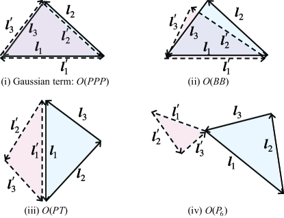
Figure 1: Illustration of the different terms of the bispectrum covariance. The triangle configurations for two bispectra in the covariance matrix, B(𝒍1,𝒍2,𝒍3)𝐵subscript𝒍1subscript𝒍2subscript𝒍3B(\mbox{$\mbox{\boldmath$l$}_{1},\mbox{\boldmath$l$}_{2},\mbox{\boldmath$l$}_{3}$}) and B(𝒍1,𝒍2,𝒍3)𝐵superscriptsubscript𝒍1subscriptsuperscript𝒍2subscriptsuperscript𝒍3B(\mbox{$\mbox{\boldmath$l$}_{1}^{\prime},\mbox{\boldmath$l$}^{\prime}_{2},\mbox{\boldmath$l$}^{\prime}_{3}$}), are specified by sets of the three vectors (𝒍1,𝒍2,𝒍3)subscript𝒍1subscript𝒍2subscript𝒍3(\mbox{$\mbox{\boldmath$l$}_{1},\mbox{\boldmath$l$}_{2},\mbox{\boldmath$l$}_{3}$}) or (𝒍1,𝒍2,𝒍3)superscriptsubscript𝒍1subscriptsuperscript𝒍2subscriptsuperscript𝒍3(\mbox{$\mbox{\boldmath$l$}_{1}^{\prime},\mbox{\boldmath$l$}^{\prime}_{2},\mbox{\boldmath$l$}^{\prime}_{3}$}), denoted by the solid and dashed lines, respectively. The three vectors satisfy the triangle conditions 𝒍1+𝒍2+𝒍3=𝟎subscript𝒍1subscript𝒍2subscript𝒍30\mbox{\boldmath$l$}_{1}+\mbox{\boldmath$l$}_{2}+\mbox{\boldmath$l$}_{3}=\mbox{\boldmath$0$} and 𝒍1+𝒍2+𝒍3=𝟎superscriptsubscript𝒍1superscriptsubscript𝒍2superscriptsubscript𝒍30\mbox{\boldmath$l$}_{1}^{\prime}+\mbox{\boldmath$l$}_{2}^{\prime}+\mbox{\boldmath$l$}_{3}^{\prime}=\mbox{\boldmath$0$}. (i) The Gaussian part of the bispectrum covariance, which arises only if the two triangle configurations have the same shape (within the coarseness of the bin widths). The two vectors with the same length but in the opposite direction such as 𝒍1subscript𝒍1\mbox{\boldmath$l$}_{1} and 𝒍1superscriptsubscript𝒍1\mbox{\boldmath$l$}_{1}^{\prime} yield the power spectrum after the ensemble average. Hence the Gaussian term amplitude is proportional to P(l1)P(l2)P(l3)𝑃subscript𝑙1𝑃subscript𝑙2𝑃subscript𝑙3P(l_{1})P(l_{2})P(l_{3}) and contributes to the diagonal terms of the covariance matrix. (ii) Non-Gaussian part of the bispectrum covariance which arises if one side of the two triangles is in the same length and direction; here 𝒍1=𝒍1subscript𝒍1superscriptsubscript𝒍1\mbox{\boldmath$l$}_{1}=\mbox{\boldmath$l$}_{1}^{\prime} is shown as an example. The amplitude of this covariance term is proportional to B(l1,l2,l3)B(l1,l2,l3)𝐵subscript𝑙1subscript𝑙2subscript𝑙3𝐵subscriptsuperscript𝑙1superscriptsubscript𝑙2superscriptsubscript𝑙3B(l_{1},l_{2},l_{3})B(l^{\prime}_{1},l_{2}^{\prime},l_{3}^{\prime}). (iii) Non-Gaussian part that arises if one side length of the two triangles is the same but in the opposite direction, 𝒍1=𝒍1subscript𝒍1superscriptsubscript𝒍1\mbox{\boldmath$l$}_{1}=-\mbox{\boldmath$l$}_{1}^{\prime}. The amplitude is O(PT)𝑂𝑃𝑇O(PT); the figure shows a case of P(l1)T(𝒍1,𝒍3,𝒍2,𝒍3)𝑃subscript𝑙1𝑇subscript𝒍1subscript𝒍3superscriptsubscript𝒍2superscriptsubscript𝒍3P(l_{1})T(\mbox{\boldmath$l$}_{1},\mbox{\boldmath$l$}_{3},\mbox{\boldmath$l$}_{2}^{\prime},\mbox{\boldmath$l$}_{3}^{\prime}). The surrounding four vectors (𝒍2,𝒍3,𝒍2,𝒍3subscript𝒍2subscript𝒍3superscriptsubscript𝒍2superscriptsubscript𝒍3\mbox{\boldmath$l$}_{2},\mbox{\boldmath$l$}_{3},\mbox{\boldmath$l$}_{2}^{\prime},\mbox{\boldmath$l$}_{3}^{\prime} ) form a quadrangular configuration satisfying the condition 𝒍2+𝒍3+𝒍2+𝒍3=𝟎subscript𝒍2subscript𝒍3superscriptsubscript𝒍2superscriptsubscript𝒍30\mbox{\boldmath$l$}_{2}+\mbox{\boldmath$l$}_{3}+\mbox{\boldmath$l$}_{2}^{\prime}+\mbox{\boldmath$l$}_{3}^{\prime}=\mbox{\boldmath$0$}, which gives the trispectrum contribution. (iv) Non-Gaussian part which arises for generic triangle configurations and therefore contributes to all diagonal and off-diagonal terms of the covariance matrix. The amplitude is proportional to the connected part of the six-point correlation function, P6subscript𝑃6P_{6}. As indicated, the 6 vectors of (𝒍1,𝒍2,𝒍3,𝒍1,𝒍2,𝒍3subscript𝒍1subscript𝒍2subscript𝒍3superscriptsubscript𝒍1subscriptsuperscript𝒍2subscriptsuperscript𝒍3\mbox{\boldmath$l$}_{1},\mbox{\boldmath$l$}_{2},\mbox{\boldmath$l$}_{3},\mbox{$\mbox{\boldmath$l$}_{1}^{\prime},\mbox{\boldmath$l$}^{\prime}_{2},\mbox{\boldmath$l$}^{\prime}_{3}$}) arise from the two triangles that form the six-point configuration in Fourier space, although the two vertices of the 6 points are collapsed to one point due to the triangle conditions.

We present the detailed derivation of the bispectrum covariance in Appendix A based on the discrete Fourier decomposition formulation. Here we just give the expression of the bispectrum covariance, which has three contributions, the Gaussian and non-Gaussian errors and the HSV contribution:

Cov[B(l1,l2,l3),B(l1,l2,l3)]Cov𝐵subscript𝑙1subscript𝑙2subscript𝑙3𝐵superscriptsubscript𝑙1superscriptsubscript𝑙2superscriptsubscript𝑙3\displaystyle{\rm Cov}\left[B(l_{1},l_{2},l_{3}),B(l_{1}^{\prime},l_{2}^{\prime},l_{3}^{\prime})\right] =\displaystyle= CovGauss+CovNG+CovHSVBBsubscriptCovGausssubscriptCovNGsubscriptsuperscriptCov𝐵𝐵HSV\displaystyle{\rm Cov}_{\rm Gauss}+{\rm Cov}_{\rm NG}+{\rm Cov}^{BB}_{\rm HSV} (18)
=\displaystyle= ΩsNtrip(l1,l2,l3)P(l1)P(l2)P(l3)[δl1l1Kδl2l2Kδl3l3K+δl1l1Kδl2l3Kδl3l2K+δl1l2Kδl2l1Kδl3l3K+3 perms.]subscriptΩssubscript𝑁tripsubscript𝑙1subscript𝑙2subscript𝑙3𝑃subscript𝑙1𝑃subscript𝑙2𝑃subscript𝑙3delimited-[]subscriptsuperscript𝛿𝐾subscript𝑙1superscriptsubscript𝑙1subscriptsuperscript𝛿𝐾subscript𝑙2superscriptsubscript𝑙2subscriptsuperscript𝛿𝐾subscript𝑙3superscriptsubscript𝑙3subscriptsuperscript𝛿𝐾subscript𝑙1superscriptsubscript𝑙1subscriptsuperscript𝛿𝐾subscript𝑙2superscriptsubscript𝑙3subscriptsuperscript𝛿𝐾subscript𝑙3superscriptsubscript𝑙2subscriptsuperscript𝛿𝐾subscript𝑙1superscriptsubscript𝑙2subscriptsuperscript𝛿𝐾subscript𝑙2superscriptsubscript𝑙1subscriptsuperscript𝛿𝐾subscript𝑙3superscriptsubscript𝑙33 perms.\displaystyle\frac{\Omega_{\rm s}}{N_{\rm trip}(l_{1},l_{2},l_{3})}P(l_{1})P(l_{2})P(l_{3})\left[\delta^{K}_{l_{1}l_{1}^{\prime}}\delta^{K}_{l_{2}l_{2}^{\prime}}\delta^{K}_{l_{3}l_{3}^{\prime}}+\delta^{K}_{l_{1}l_{1}^{\prime}}\delta^{K}_{l_{2}l_{3}^{\prime}}\delta^{K}_{l_{3}l_{2}^{\prime}}+\delta^{K}_{l_{1}l_{2}^{\prime}}\delta^{K}_{l_{2}l_{1}^{\prime}}\delta^{K}_{l_{3}l_{3}^{\prime}}+\mbox{3 perms.}\right]
+2πΩsB(l1,l2,l3)B(l1,l2,l3)[δl1l1Kl1Δl1+δl1l2Kl1Δl1+7 perms.]2𝜋subscriptΩs𝐵subscript𝑙1subscript𝑙2subscript𝑙3𝐵superscriptsubscript𝑙1superscriptsubscript𝑙2superscriptsubscript𝑙3delimited-[]subscriptsuperscript𝛿𝐾subscript𝑙1superscriptsubscript𝑙1subscript𝑙1Δsubscript𝑙1subscriptsuperscript𝛿𝐾subscript𝑙1superscriptsubscript𝑙2subscript𝑙1Δsubscript𝑙17 perms.\displaystyle+\frac{2\pi}{\Omega_{\rm s}}B(l_{1},l_{2},l_{3})B(l_{1}^{\prime},l_{2}^{\prime},l_{3}^{\prime})\left[\frac{\delta^{K}_{l_{1}l_{1}^{\prime}}}{l_{1}\Delta l_{1}}+\frac{\delta^{K}_{l_{1}l_{2}^{\prime}}}{{l_{1}\Delta l_{1}}}+\mbox{7 perms.}\right]
+δl1l1K2πΩsl1Δl1P(l1)T(𝒍2,𝒍3,𝒍2,𝒍3)+δl1l2K2πΩsl1Δl1P(l1)T(𝒍2,𝒍3,𝒍1,𝒍3)+7 perms.subscriptsuperscript𝛿𝐾subscript𝑙1superscriptsubscript𝑙12𝜋subscriptΩssubscript𝑙1Δsubscript𝑙1𝑃subscript𝑙1𝑇subscript𝒍2subscript𝒍3superscriptsubscript𝒍2superscriptsubscript𝒍3subscriptsuperscript𝛿𝐾subscript𝑙1superscriptsubscript𝑙22𝜋subscriptΩssubscript𝑙1Δsubscript𝑙1𝑃subscript𝑙1𝑇subscript𝒍2subscript𝒍3superscriptsubscript𝒍1superscriptsubscript𝒍37 perms.\displaystyle+\delta^{K}_{l_{1}l_{1}^{\prime}}\frac{2\pi}{\Omega_{\rm s}l_{1}\Delta l_{1}}P(l_{1})T(\mbox{\boldmath$l$}_{2},\mbox{\boldmath$l$}_{3},\mbox{\boldmath$l$}_{2}^{\prime},\mbox{\boldmath$l$}_{3}^{\prime})+\delta^{K}_{l_{1}l_{2}^{\prime}}\frac{2\pi}{\Omega_{\rm s}l_{1}\Delta l_{1}}P(l_{1})T(\mbox{\boldmath$l$}_{2},\mbox{\boldmath$l$}_{3},\mbox{\boldmath$l$}_{1}^{\prime},\mbox{\boldmath$l$}_{3}^{\prime})+\mbox{7 perms.}
+1Ωsdψ2πP6(𝒍1,𝒍2,𝒍3,𝒍1,𝒍2,𝒍3;ψ)1subscriptΩs𝑑𝜓2𝜋subscript𝑃6subscript𝒍1subscript𝒍2subscript𝒍3superscriptsubscript𝒍1superscriptsubscript𝒍2superscriptsubscript𝒍3𝜓\displaystyle+\frac{1}{\Omega_{\rm s}}\int\!\!\frac{d\psi}{2\pi}~{}P_{6}(\mbox{\boldmath$l$}_{1},\mbox{\boldmath$l$}_{2},\mbox{\boldmath$l$}_{3},\mbox{\boldmath$l$}_{1}^{\prime},\mbox{\boldmath$l$}_{2}^{\prime},\mbox{\boldmath$l$}_{3}^{\prime};\psi)
+CovHSVBB,superscriptsubscriptCovHSV𝐵𝐵\displaystyle+{\rm Cov}_{\rm HSV}^{BB},

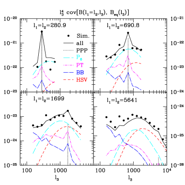
where the notation ‘NG’ stands for the ‘non-Gaussian’ error contribution, and P6subscript𝑃6P_{6} denotes the connected part of the six-point correlation function. Fig. 1 shows a diagram picture of these covariance terms from the first to the fourth lines on the r.h.s. of equation (18). When further including the intrinsic shape noise contribution, we just replace the power spectra in the terms of the above equation (O(P3)𝑂superscript𝑃3O(P^{3}) and O(PT)𝑂𝑃𝑇O(PT) terms) with the power spectrum including the shot noise contribution (equation 10).

The terms of the first line on the r.h.s. are the Gaussian covariance terms, which contribute only to the diagonal terms of the bispectrum covariances. The combination of the Kronecker deltas δl1l1Kδl2l2Kδl3l3Ksubscriptsuperscript𝛿𝐾subscript𝑙1superscriptsubscript𝑙1subscriptsuperscript𝛿𝐾subscript𝑙2superscriptsubscript𝑙2subscriptsuperscript𝛿𝐾subscript𝑙3superscriptsubscript𝑙3\delta^{K}_{l_{1}l_{1}^{\prime}}\delta^{K}_{l_{2}l_{2}^{\prime}}\delta^{K}_{l_{3}l_{3}^{\prime}} is non-vanishing only if the two triangle configurations are in the same “shape” within the bin widths. In particular, if triangle configurations have symmetry such as isosceles or equilateral triangles, the combination of Kronecker deltas (the terms in the square bracket on the first line) yield a factor of 2 or 6 for isosceles and equilateral triangles, respectively. The factors account for the fact that different triangles transformed by parity and permutation transformations (liljsubscript𝑙𝑖superscriptsubscript𝑙𝑗l_{i}\leftrightarrow l_{j}^{\prime}) are not independent for a statistically homogeneous and isotropic field. For a general triangle configuration liljsubscript𝑙𝑖subscript𝑙𝑗l_{i}\neq l_{j}, the factor becomes unity. The prefactor Ntrip(l1,l2,l3)subscript𝑁tripsubscript𝑙1subscript𝑙2subscript𝑙3N_{\rm trip}(l_{1},l_{2},l_{3}) is given by equation (16).

The terms from the second to the fourth lines are the non-Gaussian error contributions, which arise from the higher-order correlation functions of the lensing field. The coefficient of each term such as 2π/(Ωsl1Δl1)2𝜋subscriptΩssubscript𝑙1Δsubscript𝑙12\pi/(\Omega_{\rm s}l_{1}\Delta l_{1}) is from the number of independent configurations in Fourier space that form a given configuration of six wavevectors (𝒍1,𝒍2,𝒍3,𝒍1,𝒍2,𝒍3subscript𝒍1subscript𝒍2subscript𝒍3superscriptsubscript𝒍1subscriptsuperscript𝒍2subscriptsuperscript𝒍3\mbox{$\mbox{\boldmath$l$}_{1},\mbox{\boldmath$l$}_{2},\mbox{\boldmath$l$}_{3}$},\mbox{$\mbox{\boldmath$l$}_{1}^{\prime},\mbox{\boldmath$l$}^{\prime}_{2},\mbox{\boldmath$l$}^{\prime}_{3}$}) in Fig. 1 (also see Appendix A for the mathematical derivation). The angular integration in the fourth term including P6subscript𝑃6P_{6} is over the angle ψ𝜓\psi between the vectors 𝒍1subscript𝒍1\mbox{\boldmath$l$}_{1} and 𝒍1superscriptsubscript𝒍1\mbox{\boldmath$l$}_{1}^{\prime} in order to include contributions over all the possible six-point configurations in Fourier space. Note that the terms in the first, second and third lines on the r.h.s. depend on the multipole bin widths such as Δl1Δsubscript𝑙1\Delta l_{1}, while the term including P6subscript𝑃6P_{6} and the HSV do not depend on the bin widths.

As in the power spectrum covariance (equation 11), the number fluctuations of massive haloes due to the large-scale mass fluctuations affect the bispectrum estimated from a finite area survey. The HSV contribution to the bispectrum covariance is given as

Cov[Bκ(𝒍1,𝒍2,𝒍3),Bκ(𝒍1,𝒍2,𝒍3)]HSVCovsubscriptsubscript𝐵𝜅subscript𝒍1subscript𝒍2subscript𝒍3subscript𝐵𝜅subscriptsuperscript𝒍1subscriptsuperscript𝒍2subscriptsuperscript𝒍3HSV\displaystyle{\rm Cov}[B_{\kappa}(\mbox{\boldmath$l$}_{1},\mbox{\boldmath$l$}_{2},\mbox{\boldmath$l$}_{3}),B_{\kappa}(\mbox{\boldmath$l$}^{\prime}_{1},\mbox{\boldmath$l$}^{\prime}_{2},\mbox{\boldmath$l$}^{\prime}_{3})]_{\rm HSV} =\displaystyle= 𝑑χ(d2VdχdΩ)2[𝑑MdndMb(M)κ~M(l1)κ~M(l2)κ~M(l3)]differential-d𝜒superscriptsuperscript𝑑2𝑉𝑑𝜒𝑑Ω2delimited-[]differential-d𝑀𝑑𝑛𝑑𝑀𝑏𝑀subscript~𝜅𝑀subscript𝑙1subscript~𝜅𝑀subscript𝑙2subscript~𝜅𝑀subscript𝑙3\displaystyle\int\!d\chi\left(\frac{d^{2}V}{d\chi d\Omega}\right)^{2}\left[\int\!dM\frac{dn}{dM}b(M)\tilde{\kappa}_{M}(l_{1})\tilde{\kappa}_{M}(l_{2})\tilde{\kappa}_{M}(l_{3})\right] (19)
×[𝑑MdndMb(M)κ~M(l1)κ~M(l2)κ~M(l3)]kdk2πPmL(k;χ)|W~(kχΘs)|2.absentdelimited-[]differential-dsuperscript𝑀𝑑𝑛𝑑superscript𝑀𝑏superscript𝑀subscript~𝜅superscript𝑀subscriptsuperscript𝑙1subscript~𝜅superscript𝑀subscriptsuperscript𝑙2subscript~𝜅superscript𝑀subscriptsuperscript𝑙3𝑘𝑑𝑘2𝜋superscriptsubscript𝑃𝑚𝐿𝑘𝜒superscript~𝑊𝑘𝜒subscriptΘ𝑠2\displaystyle\times\left[\int\!dM^{\prime}\frac{dn}{dM^{\prime}}b(M^{\prime})\tilde{\kappa}_{M^{\prime}}(l^{\prime}_{1})\tilde{\kappa}_{M^{\prime}}(l^{\prime}_{2})\tilde{\kappa}_{M^{\prime}}(l^{\prime}_{3})\right]\int\frac{kdk}{2\pi}P_{m}^{L}\left(k;\chi\right)\left|\tilde{W}(k\chi\Theta_{s})\right|^{2}.

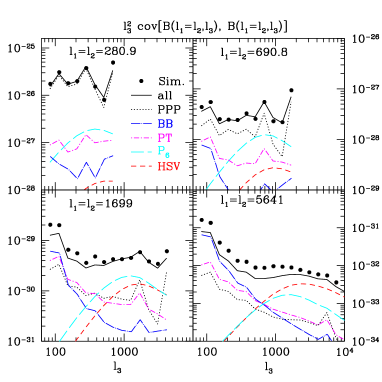
This contribution has not been realized in previous works. By comparing with ray-tracing simulations, we will show below that the HSV contribution is dominant over other covariance terms at l1000greater-than-or-similar-to𝑙1000l\ga 1000, in the non-linear regime, and adding the HSV term to the model predictions significantly improves agreement with the simulation results. Again note that the HSV term scales with the survey area in a non-trivial way via the linear mass power spectrum (see the discussion below equation 14), while the other terms scale with survey area as 1/Ωs1subscriptΩs1/\Omega_{\rm s}.

Refer to caption
Refer to caption
Refer to caption
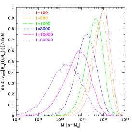
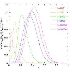
Figure 2: Left-hand panel: the plot shows how haloes of different masses contribute to the halo sample variance (HSV) terms of the bispectrum covariance for a given equilateral triangle configuration. We used the halo model expression (equation 19) to compute the fractional contributions. For the triangle with side length l=1000𝑙1000l=1000, haloes with masses 1014Mgreater-than-or-similar-toabsentsuperscript1014subscript𝑀direct-product\ga 10^{14}M_{\odot} dominate the contribution to the HSV. Middle: Similar plot, but for the redshift distribution of the bispectrum covariance. For the triangle with l=1000𝑙1000l=1000, haloes at z0.4less-than-or-similar-to𝑧0.4z\la 0.4 give the dominant contribution. Right: The survey area dependence of the HSV contribution for the power spectrum and the bispectrum, relative to that of the Gaussian error, which scales as CovGauss1/Ωsproportional-tosubscriptCovGauss1subscriptΩs{\rm Cov}_{\rm Gauss}\propto 1/\Omega_{\rm s}. Here we consider the scale of l=2000𝑙2000l=2000 for P(l)𝑃𝑙P(l) and Beq(l)subscript𝐵eq𝑙B_{\rm eq}(l), employ the flat sky approximation, and assume the survey geometry given by Ωs=πΘs2subscriptΩs𝜋superscriptsubscriptΘs2\Omega_{\rm s}=\pi\Theta_{\rm s}^{2}.

The left-hand and middle panels of Fig. 2 show which haloes of mass and redshift range contribute to the HSV term of the bispectrum covariance for an equilateral triangle configuration of a given side length. For the triangle with l=1000𝑙1000l=1000, haloes with masses 1014Mgreater-than-or-similar-toabsentsuperscript1014subscript𝑀direct-product\ga 10^{14}M_{\odot} and at redshift z0.4less-than-or-similar-to𝑧0.4z\la 0.4 give a dominant contribution to the HSV effect. These haloes are relatively easy to be identified from a concentration of galaxies on the sky, X-ray or the Sunyaev–Zel’dovich effect. In other words, identifying such massive haloes in a survey region and comparing the number with the expected number for a fiducial cosmological model will help understand the HSV effect for the weak lensing observables in the survey region (also see Takada & Bridle 2007, for the similar discussion). The right-hand panel shows how the HSV terms scale with the survey area, in comparison with the Gaussian covariance term for the power spectrum covariance and the bispectrum covariance of equilateral triangles. Here we consider the particular multipole bin l=2000𝑙2000l=2000, and assume the flat-sky approximation and a circular survey geometry, Ωs=πΘs2subscriptΩs𝜋superscriptsubscriptΘs2\Omega_{\rm s}=\pi\Theta_{\rm s}^{2}, for simplicity. The plot shows that the HSV term decreases more slowly than other terms as ΩssubscriptΩs\Omega_{\rm s} increases up to a few 100 deg2.

3.3 Cross-covariance between power spectrum and bispectrum

Since the power spectrum and bispectrum are not independent for the non-Gaussian field, we need to account for the cross-covariance between the two observables in order not to double-count the information content. We can derive the cross-covariance (see Appendix B) similarly to the power spectrum and the bispectrum covariance as

Cov[Pest(l),Best(l1,l2,l3)]Covsuperscript𝑃est𝑙superscript𝐵estsubscript𝑙1subscript𝑙2subscript𝑙3\displaystyle{\rm Cov}\left[P^{\rm est}(l),B^{\rm est}(l_{1},l_{2},l_{3})\right] =\displaystyle= CovNGPB+CovHSVPBsubscriptsuperscriptCov𝑃𝐵𝑁𝐺subscriptsuperscriptCov𝑃𝐵HSV\displaystyle{\rm Cov}^{PB}_{NG}+{\rm Cov}^{PB}_{\rm HSV} (20)
=\displaystyle= δll1K4πΩsl1Δl1P(l)B(l,l2,l3)+2 perms.+1Ωsdψ2πP5(𝒍,𝒍,𝒍1,𝒍2,𝒍3;ψ)+CovHSVPB,subscriptsuperscript𝛿𝐾𝑙subscript𝑙14𝜋subscriptΩssubscript𝑙1Δsubscript𝑙1𝑃𝑙𝐵𝑙subscript𝑙2subscript𝑙32 perms.1subscriptΩs𝑑𝜓2𝜋subscript𝑃5𝒍𝒍subscript𝒍1subscript𝒍2subscript𝒍3𝜓subscriptsuperscriptCov𝑃𝐵HSV\displaystyle\delta^{K}_{ll_{1}}\frac{4\pi}{\Omega_{\rm s}l_{1}\Delta l_{1}}P(l)B(l,l_{2},l_{3})+\mbox{2 perms.}+\frac{1}{\Omega_{\rm s}}\int\!\frac{d\psi}{2\pi}~{}P_{5}(\mbox{\boldmath$l$},-\mbox{\boldmath$l$},\mbox{\boldmath$l$}_{1},\mbox{\boldmath$l$}_{2},\mbox{\boldmath$l$}_{3};\psi)+{\rm Cov}^{PB}_{\rm HSV},

where P5subscript𝑃5P_{5} is the five-point correlation function, and ψ𝜓\psi is the angle between the vectors 𝒍𝒍l and 𝒍1subscript𝒍1\mbox{\boldmath$l$}_{1} as in equation (18). The HSV term is given as

Cov[Pκ(l),Bκ(𝒍1,𝒍2,𝒍3),]HSV\displaystyle{\rm Cov}[P_{\kappa}(l),B_{\kappa}(\mbox{\boldmath$l$}_{1},\mbox{\boldmath$l$}_{2},\mbox{\boldmath$l$}_{3}),]_{\rm HSV} =\displaystyle= 𝑑χ(d2VdχdΩ)2[𝑑mdndMb(M)|κ~M(l)|2]differential-d𝜒superscriptsuperscript𝑑2𝑉𝑑𝜒𝑑Ω2delimited-[]differential-d𝑚𝑑𝑛𝑑𝑀𝑏𝑀superscriptsubscript~𝜅𝑀𝑙2\displaystyle\int\!d\chi\left(\frac{d^{2}V}{d\chi d\Omega}\right)^{2}\left[\int\!dm\frac{dn}{dM}b(M)\left|\tilde{\kappa}_{M}(l)\right|^{2}\right] (21)
×[𝑑MdndMb(M)κ~M(l1)κ~M(l2)κ~M(l3)]kdk2πPmL(k;χ)|W~(kχΘs)|2.absentdelimited-[]differential-d𝑀𝑑𝑛𝑑superscript𝑀𝑏superscript𝑀subscript~𝜅superscript𝑀subscript𝑙1subscript~𝜅superscript𝑀subscript𝑙2subscript~𝜅superscript𝑀subscript𝑙3𝑘𝑑𝑘2𝜋superscriptsubscript𝑃𝑚𝐿𝑘𝜒superscript~𝑊𝑘𝜒subscriptΘ𝑠2\displaystyle\times\left[\int\!dM\frac{dn}{dM^{\prime}}b(M^{\prime})\tilde{\kappa}_{M^{\prime}}(l_{1})\tilde{\kappa}_{M^{\prime}}(l_{2})\tilde{\kappa}_{M^{\prime}}(l_{3})\right]\int\frac{kdk}{2\pi}P_{m}^{L}\left(k;\chi\right)\left|\tilde{W}(k\chi\Theta_{s})\right|^{2}.

We will use these equations when computing the total information content for a combined measurement of the lensing power spectrum and bispectrum for a given survey.

3.4 Halo sample variance contribution to the n𝑛n-point correlation function measurement

As we have seen for the HSV contributions to the lensing spectrum covariances (equations 14, 19 and 21), the equations have similar forms at the small-angle limit, where the one-halo term is dominated in the halo model picture. Extending these findings, we can find the HSV contribution to the covariance matrix between any n𝑛n- and nsuperscript𝑛n^{\prime}-point correlation functions in Fourier space:

Cov[Pn(𝒍1,𝒍2,,𝒍n),Pn(𝒍1,𝒍2,,𝒍n)]HSVCovsubscriptsubscript𝑃𝑛subscript𝒍1subscript𝒍2subscript𝒍𝑛subscript𝑃superscript𝑛superscriptsubscript𝒍1superscriptsubscript𝒍2superscriptsubscript𝒍superscript𝑛HSV\displaystyle{\rm Cov}[P_{n}(\mbox{\boldmath$l$}_{1},\mbox{\boldmath$l$}_{2},\dots,\mbox{\boldmath$l$}_{n}),P_{n^{\prime}}(\mbox{\boldmath$l$}_{1}^{\prime},\mbox{\boldmath$l$}_{2}^{\prime},\dots,\mbox{\boldmath$l$}_{n^{\prime}}^{\prime})]_{\rm HSV} =\displaystyle= 𝑑χ(d2VdχdΩ)2[𝑑MdndMb(M)κ~M(l1)κ~M(l2)κ~M(ln)]differential-d𝜒superscriptsuperscript𝑑2𝑉𝑑𝜒𝑑Ω2delimited-[]differential-d𝑀𝑑𝑛𝑑𝑀𝑏𝑀subscript~𝜅𝑀subscript𝑙1subscript~𝜅𝑀subscript𝑙2subscript~𝜅𝑀subscript𝑙𝑛\displaystyle\int\!d\chi\left(\frac{d^{2}V}{d\chi d\Omega}\right)^{2}\left[\int\!dM\frac{dn}{dM}b(M)\tilde{\kappa}_{M}(l_{1})\tilde{\kappa}_{M}(l_{2})\cdots\tilde{\kappa}_{M}(l_{n})\right] (22)
×[𝑑MdndMb(M)κ~M(l1)κ~M(l2)κ~M(ln)]kdk2πPmL(k;χ)|W~(kχΘs)|2.absentdelimited-[]differential-d𝑀𝑑𝑛𝑑superscript𝑀𝑏superscript𝑀subscript~𝜅superscript𝑀superscriptsubscript𝑙1subscript~𝜅superscript𝑀superscriptsubscript𝑙2subscript~𝜅superscript𝑀superscriptsubscript𝑙superscript𝑛𝑘𝑑𝑘2𝜋superscriptsubscript𝑃𝑚𝐿𝑘𝜒superscript~𝑊𝑘𝜒subscriptΘ𝑠2\displaystyle\times\left[\int\!dM\frac{dn}{dM^{\prime}}b(M^{\prime})\tilde{\kappa}_{M^{\prime}}(l_{1}^{\prime})\tilde{\kappa}_{M^{\prime}}(l_{2}^{\prime})\cdots\tilde{\kappa}_{M^{\prime}}(l_{n^{\prime}}^{\prime})\right]\int\frac{kdk}{2\pi}P_{m}^{L}\left(k;\chi\right)\left|\tilde{W}(k\chi\Theta_{s})\right|^{2}.

Roughly speaking, the amplitude of the HSV term simply scales as CovHSVPn1h(li)Pn1h(lj)σm2(Θs)similar-tosubscriptCovHSVsubscriptsuperscript𝑃1h𝑛subscript𝑙𝑖subscriptsuperscript𝑃1hsuperscript𝑛superscriptsubscript𝑙𝑗superscriptsubscript𝜎𝑚2subscriptΘ𝑠{\rm Cov}_{\rm HSV}\sim P^{\rm 1h}_{n}(l_{i})P^{\rm 1h}_{n^{\prime}}(l_{j}^{\prime})\sigma_{m}^{2}(\Theta_{s}). Thus any n𝑛n-point correlation functions at small angle scales can be affected by the large-scale mass fluctuations of scales comparable with or outside the survey area.

We should also emphasize that the HSV contribution affects measurements of any two- or three-dimensional correlation functions from a finite area survey, and can be very important if one is interested in the small-scale signals which are sensitive to the abundance of haloes in the finite survey region (e.g. see Shaw et al. 2009; Zhang & Sheth 2007, for a similar discussion on the SZ power spectrum measurement).

3.5 Halo model predictions for the lensing covariances

As we have described up to the preceding section, the power spectrum and bispectrum covariance calculations require to compute the four-, five- and six-point correlation functions in addition to the power spectrum and bispectrum. For the power spectrum and bispectrum, some theoretical models are proposed by comparing with simulations, e.g. Smith et al. (2003) and Valageas & Nishimichi (2011a) for the power spectrum and Scoccimarro & Frieman (1999) and Valageas & Nishimichi (2011b) for the bispectrum. The higher-order functions are, however, fairly uncertain because there are fewer studies to compare the model predictions with simulations (see e.g. Takada & Jain 2002, for an attempt to compute the kurtosis which is the collapsed four-point function), partly because the higher-order correlations require a substantial amount of computational costs. Instead of pursuing a reliable model for the higher-order correlation functions, in this paper we employ the halo model approach to compute the higher-order functions (Peacock & Smith 2000; Seljak 2000; Ma & Fry 2000; Scoccimarro et al. 2001; Cooray & Sheth 2002) in which the correlations of the mass distribution are expressed as two separate contributions: correlations of dark matter particles within the same halo and correlations between particles in different haloes. We have found that, up to the four-point correlation functions, the halo model predictions are accurate at 10–30 per cent level in the amplitude compared to N-body simulations (in particular for lensing fields; Takada & Jain 2002, 2003a, 2003b). Since our purpose of this paper is to assess the importance of non-Gaussian error contributions to the bispectrum covariance matrices, we consider that the halo model approach is adequate enough.

We know that most of the lensing information comes from small angle scales in the non-linear clustering regime to which the one-halo term, the correlation arising from the same halo, provides a dominant contribution. In addition, the non-Gaussian errors are important only at the small scales, as can be explicitly found from fig. 5 in Sato et al. (2009). For these reasons, we include only the one-halo terms to compute the non-Gaussian error contributions to the lensing covariances, which significantly simplifies the computation. Although the n𝑛n-point correlation function depends on n𝑛n wavevectors such as Pn(𝒍1,𝒍2,,𝒍n)subscript𝑃𝑛subscript𝒍1subscript𝒍2subscript𝒍𝑛P_{n}(\mbox{\boldmath$l$}_{1},\mbox{\boldmath$l$}_{2},\dots,\mbox{\boldmath$l$}_{n}), the one-halo term does not depend on any angle between the vectors, but rather depends only on the length of each vector; Pn1h(𝒍1,𝒍2,,𝒍n)=Pn1h(l1,l2,,ln)superscriptsubscript𝑃𝑛1hsubscript𝒍1subscript𝒍2subscript𝒍𝑛superscriptsubscript𝑃𝑛1hsubscript𝑙1subscript𝑙2subscript𝑙𝑛P_{n}^{\rm 1h}(\mbox{\boldmath$l$}_{1},\mbox{\boldmath$l$}_{2},\dots,\mbox{\boldmath$l$}_{n})=P_{n}^{\rm 1h}(l_{1},l_{2},\dots,l_{n}), reflecting spherical mass distribution around halo in a statistical average sense. To be more explicit, assuming the Limber’s approximation, the one-halo term of the n𝑛n-point correlation function can be computed as follows (see around equation 30 in Takada & Jain 2003a):

Pn1h(l1,l2,,ln)=0χs𝑑χd2VdχdΩ𝑑MdndMκ~M(l1)κ~M(l2)κ~M(ln).subscriptsuperscript𝑃1h𝑛subscript𝑙1subscript𝑙2subscript𝑙𝑛superscriptsubscript0subscript𝜒𝑠differential-d𝜒superscript𝑑2𝑉𝑑𝜒𝑑Ωdifferential-d𝑀𝑑𝑛𝑑𝑀subscript~𝜅𝑀subscript𝑙1subscript~𝜅𝑀subscript𝑙2subscript~𝜅𝑀subscript𝑙𝑛P^{\rm 1h}_{n}(l_{1},l_{2},\dots,l_{n})=\int_{0}^{\chi_{s}}\!\!d\chi\frac{d^{2}V}{d\chi d\Omega}\int\!dM\frac{dn}{dM}\mbox{$\tilde{\kappa}$}_{M}(l_{1})\mbox{$\tilde{\kappa}$}_{M}(l_{2})\cdots\mbox{$\tilde{\kappa}$}_{M}(l_{n}). (23)

The one-halo term is computed by a two-dimensional integration, as the Fourier transform of the lensing field due to an NFW halo, κ~M(l)subscript~𝜅𝑀𝑙\mbox{$\tilde{\kappa}$}_{M}(l), can be computed analytically for a given halo with mass M𝑀M and at redshift z𝑧z.

As can be found from equations (11), (18) and (20), some of the non-Gaussian terms can be further simplified; e.g. one of the non-Gaussian terms in the power spectrum covariance (equation 11) can be simplified as

1Ωs|𝒍|lid2𝒍A(li)|𝒍|ljd2𝒍A(lj)T(𝒍,𝒍,𝒍,𝒍)1ΩsT1h(li,li,lj,lj),similar-to-or-equals1subscriptΩssubscript𝒍subscript𝑙𝑖superscript𝑑2𝒍𝐴subscript𝑙𝑖subscriptsuperscript𝒍subscript𝑙𝑗superscript𝑑2superscript𝒍𝐴subscript𝑙𝑗𝑇𝒍𝒍superscript𝒍superscript𝒍1subscriptΩ𝑠superscript𝑇1hsubscript𝑙𝑖subscript𝑙𝑖subscript𝑙𝑗subscript𝑙𝑗\frac{1}{\Omega_{\rm s}}\int_{\left|\mbox{\boldmath$l$}\right|\in l_{i}}\!\frac{d^{2}\mbox{\boldmath$l$}}{A(l_{i})}\int_{\left|\mbox{\boldmath$l$}^{\prime}\right|\in l_{j}}\!\frac{d^{2}\mbox{\boldmath$l$}^{\prime}}{A(l_{j})}T(\mbox{\boldmath$l$},-\mbox{\boldmath$l$},\mbox{\boldmath$l$}^{\prime},-\mbox{\boldmath$l$}^{\prime})\simeq\frac{1}{\Omega_{s}}T^{\rm 1h}(l_{i},l_{i},l_{j},l_{j}), (24)

where we have assumed that the lensing trispectrum does not largely change within the multipole bin ΔlΔ𝑙\Delta l around the bins lisubscript𝑙𝑖l_{i} and ljsubscript𝑙𝑗l_{j}. Thus the above approach allows a faster computation of the power spectrum and bispectrum covariances.

4 Results: Comparison with ray-tracing simulations

4.1 Ray-tracing simulations

To study the lensing covariance matrices, we use 1000 realizations of ray-tracing simulations for a ΛΛ\LambdaCDM model in Sato et al. (2009). Although the simulations were done for various source redshifts ranging from zs=0.6subscript𝑧𝑠0.6z_{s}=0.6 to 3, we use the outputs of zs=1subscript𝑧𝑠1z_{s}=1 in this paper. In brief, each realization has an area of 5×5555\times 5 deg2 (Ωs=0.0076subscriptΩs0.0076\Omega_{\rm s}=0.0076 sr) in square shaped geometry. The ΛΛ\LambdaCDM model adopted is characterized by cosmological parameters: the matter density parameter Ωm=0.238subscriptΩm0.238\Omega_{\rm m}=0.238, the baryon density parameter Ωb=0.042subscriptΩb0.042\Omega_{\rm b}=0.042, the initial spectral index ns=0.958subscript𝑛𝑠0.958n_{s}=0.958, the amplitude of the density fluctuations σ8=0.76subscript𝜎80.76\sigma_{8}=0.76 and the Hubble constant of H0=100hsubscript𝐻0100H_{0}=100h~{}km s-1Mpc-1 with h=0.7320.732h=0.732. The linear matter power spectrum used to set the initial conditions of N-body simulations is computed by the public code CAMB (Lewis et al. 2000). It was shown that the ray-tracing simulations are reliable to within a 5 per cent accuracy up to multipole l6000similar-to-or-equals𝑙6000l\simeq 6000 for the power spectrum and up to l4000similar-to-or-equals𝑙4000l\simeq 4000 for the bispectrum. See Sato et al. (2009) and Valageas et al. (2012) for more details.999The simulation data is available at http://www.a.phys.nagoya-u.ac.jp/~masanori/HSC/

As can be found from fig. 1 in Sato et al. (2009), the ray-tracing simulations were done in a light cone of area 5×5555\times 5 deg2, viewed from an observer position (z=0𝑧0z=0). The projected mass density fields in intermediate-redshift slices were generated from N-body simulations which have a larger simulation box than the volume covered by the light cone. Hence the lensing fields have contributions from the mass density field of scales outside the ray-tracing simulation area, although, exactly speaking, the modes outside the N-body simulation box were not included (see Appendix C for the effect). Thus the ray-tracing simulations allow us to study the HSV effect on the covariance matrices.

4.2 Measuring power spectrum, bispectrum and the covariance matrices from simulations

In each simulation realization, the lensing convergence field, κ(𝜽)𝜅𝜽\kappa(\mbox{\boldmath$\theta$}), is given on 2048×2048204820482048\times 2048 grids. We used the FFT method to compute the Fourier transformed field, κ~(𝒍)~𝜅𝒍\mbox{$\tilde{\kappa}$}(\mbox{\boldmath$l$}). The fundamental mode of the discrete Fourier decomposition is lf=72(=2π/5)subscript𝑙𝑓annotated72absent2𝜋superscript5l_{f}=72(=2\pi/5^{\circ}) and the Nyquist frequency is 70000similar-toabsent70000\sim 70000, which is large enough compared to the resolution limit of the N-body simulations. We use multipole bins that are logarithmically spaced by Δlnl=0.3(Δlogl0.13)Δ𝑙0.3similar-to-or-equalsΔ𝑙0.13\Delta\ln l=0.3~{}(\Delta\log l\simeq 0.13), which significantly reduces the number of triangle configurations (the number of different bispectra) we need to consider, compared to Δl=1Δ𝑙1\Delta l=1 as in the CMB case. We consider 16 multipole bins in total; the first bin is in the range l=[72,97.2]𝑙7297.2l=[72,97.2], and the 16th bin is in the range l=[6481.2,8748.8]𝑙6481.28748.8l=[6481.2,8748.8], so lmin=72subscript𝑙min72l_{\rm min}=72 and lmax=8748.8subscript𝑙max8748.8l_{\rm max}=8748.8.

The power spectrum of the i𝑖ith multipole bin lisubscript𝑙𝑖l_{i}, P(li)𝑃subscript𝑙𝑖P(l_{i}), is estimated from each realization by computing an azimuthal average of the estimator, κ~𝒍κ~𝒍subscript~𝜅𝒍subscript~𝜅𝒍\mbox{$\tilde{\kappa}$}_{\mbox{\boldmath$l$}}\mbox{$\tilde{\kappa}$}_{-\mbox{\boldmath$l$}}, where |𝒍|𝒍|\mbox{\boldmath$l$}| resides in the target bin. We then averaged the estimated power spectra in 1000 realizations to estimate the ensemble-averaged power spectrum (corresponding to the power spectrum for the area of 1000×25=25000100025250001000\times 25=25000 deg2). Then we computed the scatters among the power spectra of 1000 realizations in order to estimate the covariance matrix of the power spectra. Hence the covariance matrix is for an area of 25 deg2.

The bispectrum is given as a function of triangle configuration. We use three side lengths (l1,l2,l3)subscript𝑙1subscript𝑙2subscript𝑙3(l_{1},l_{2},l_{3}) to parametrize triangle configuration, where the triangle conditions are given as |ljlk|lilj+lksubscript𝑙𝑗subscript𝑙𝑘subscript𝑙𝑖subscript𝑙𝑗subscript𝑙𝑘|l_{j}-l_{k}|\leq l_{i}\leq l_{j}+l_{k}. Although the multipole bin used has a logarithmically spaced bin width, we impose the triangle conditions on the central values of the multipole bins. In addition we impose the condition l1l2l3subscript𝑙1subscript𝑙2subscript𝑙3l_{1}\leq l_{2}\leq l_{3} so that every triangle configuration is counted once. For the 16 multipole bins above, we have 204 triangle configurations in total.
Refer to caption
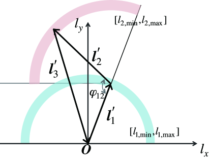
Figure 3: Illustration describing how to choose three vectors in Fourier space that satisfy triangle configurations within multipole bin widths. The triangle configuration is specified by three side lengths which have central values (l1,l2,l3subscript𝑙1subscript𝑙2subscript𝑙3l_{1},l_{2},l_{3}) and the widths Δlnl=0.3Δ𝑙0.3\Delta\ln l=0.3. The three vertices chosen are used in estimating the bispectrum from ray-tracing simulations by averaging the estimator Re[κ~𝒍1κ~𝒍2κ~𝒍3]Redelimited-[]subscript~𝜅superscriptsubscript𝒍1subscript~𝜅superscriptsubscript𝒍2subscript~𝜅superscriptsubscript𝒍3{\rm Re}[\mbox{$\tilde{\kappa}$}_{\mbox{\boldmath$l$}_{1}^{\prime}}\mbox{$\tilde{\kappa}$}_{\mbox{\boldmath$l$}_{2}^{\prime}}\mbox{$\tilde{\kappa}$}_{\mbox{\boldmath$l$}_{3}^{\prime}}] over the triangles (see text for details). First, the first vector 𝒍1superscriptsubscript𝒍1\mbox{\boldmath$l$}_{1}^{\prime} is chosen from the annulus (shaded region), which is in the upper half plane and has the radius in the range [l1,min,l1,max]subscript𝑙1minsubscript𝑙1max[l_{1,\rm min},l_{1,\rm max}] (a bin of l1subscript𝑙1l_{1}). Then, the second vector 𝒍2superscriptsubscript𝒍2\mbox{\boldmath$l$}_{2}^{\prime} is chosen from the annulus which has position angle in the range arg(𝒍1)arg(𝒍2)πsuperscriptsubscript𝒍1superscriptsubscript𝒍2𝜋\arg(\mbox{\boldmath$l$}_{1}^{\prime})\leq\arg(\mbox{\boldmath$l$}_{2}^{\prime})\leq\pi and has radius in the range [l2,min,l2,max]subscript𝑙2minsubscript𝑙2max[l_{2,\rm min},l_{2,\rm max}]. For the given pair of 𝒍1superscriptsubscript𝒍1\mbox{\boldmath$l$}_{1}^{\prime} and 𝒍2superscriptsubscript𝒍2\mbox{\boldmath$l$}_{2}^{\prime}, the third vector 𝒍3superscriptsubscript𝒍3\mbox{\boldmath$l$}_{3}^{\prime} is determined by the triangle condition 𝒍3=𝒍1𝒍2superscriptsubscript𝒍3superscriptsubscript𝒍1superscriptsubscript𝒍2\mbox{\boldmath$l$}_{3}^{\prime}=-\mbox{\boldmath$l$}_{1}^{\prime}-\mbox{\boldmath$l$}_{2}^{\prime}; if l3superscriptsubscript𝑙3l_{3}^{\prime} is in the range lminl3lmaxsubscript𝑙minsuperscriptsubscript𝑙3subscript𝑙maxl_{\rm min}\leq l_{3}^{\prime}\leq l_{\rm max}, the triplet of (𝒍1,𝒍2,𝒍3superscriptsubscript𝒍1subscriptsuperscript𝒍2subscriptsuperscript𝒍3\mbox{\boldmath$l$}_{1}^{\prime},\mbox{\boldmath$l$}^{\prime}_{2},\mbox{\boldmath$l$}^{\prime}_{3}) is accepted and otherwise discarded. The angle φ12subscript𝜑12\varphi_{12} is used for discussion in Appendix A.

For a triangle configuration that is specified by the side lengths (l1,l2,l3)subscript𝑙1subscript𝑙2subscript𝑙3(l_{1},l_{2},l_{3}) (with the bin widths), we can estimate the bispectrum from each ray-tracing simulation by averaging the estimator Re[κ~𝒍1κ~𝒍2κ~𝒍3]Redelimited-[]subscript~𝜅superscriptsubscript𝒍1subscript~𝜅superscriptsubscript𝒍2subscript~𝜅superscriptsubscript𝒍3{\rm Re}[\mbox{$\tilde{\kappa}$}_{\mbox{\boldmath$l$}_{1}^{\prime}}\mbox{$\tilde{\kappa}$}_{\mbox{\boldmath$l$}_{2}^{\prime}}\mbox{$\tilde{\kappa}$}_{\mbox{\boldmath$l$}_{3}^{\prime}}] over all the triplets (𝒍1,𝒍2,𝒍3superscriptsubscript𝒍1subscriptsuperscript𝒍2subscriptsuperscript𝒍3\mbox{\boldmath$l$}_{1}^{\prime},\mbox{\boldmath$l$}^{\prime}_{2},\mbox{\boldmath$l$}^{\prime}_{3}) which satisfy the triangle conditions; the length of each vector is in the triangle bin such as l1,minl1l1,maxsubscript𝑙1minsuperscriptsubscript𝑙1subscript𝑙1maxl_{1,\rm min}\leq l_{1}^{\prime}\leq l_{1,\rm max}. Note that, as long as the triplets of (𝒍1,𝒍2,𝒍3)superscriptsubscript𝒍1subscriptsuperscript𝒍2subscriptsuperscript𝒍3(\mbox{$\mbox{\boldmath$l$}_{1}^{\prime},\mbox{\boldmath$l$}^{\prime}_{2},\mbox{\boldmath$l$}^{\prime}_{3}$}) in Fourier space have the same side lengths l1,l2,l3subscript𝑙1subscript𝑙2subscript𝑙3l_{1},l_{2},l_{3} within the bin widths, all the triangles transformed by the rotation and parity transform are equivalent to yield the same bispectrum due to the rotation and parity invariance for a statistically homogeneous and isotropic field. In our simulations, the Fourier transformed convergence field, κ~(𝒍)~𝜅𝒍\mbox{$\tilde{\kappa}$}(\mbox{\boldmath$l$}), is given on 2048×2048204820482048\times 2048 grids in Fourier space, where the grids are linearly spaced by the fundamental mode, lf=2π/Θs=72subscript𝑙𝑓2𝜋subscriptΘs72l_{f}=2\pi/\Theta_{\rm s}=72. To have an efficient computation over 1000 realizations, we first built the table of three vectors (grids), (𝒍1,𝒍2,𝒍3)superscriptsubscript𝒍1subscriptsuperscript𝒍2subscriptsuperscript𝒍3(\mbox{$\mbox{\boldmath$l$}_{1}^{\prime},\mbox{\boldmath$l$}^{\prime}_{2},\mbox{\boldmath$l$}^{\prime}_{3}$}), where each triplet satisfies the triangle conditions (|𝒍j𝒍k|li|𝒍j+𝒍k|subscriptsuperscript𝒍𝑗subscriptsuperscript𝒍𝑘superscriptsubscript𝑙𝑖subscriptsuperscript𝒍𝑗subscriptsuperscript𝒍𝑘|\mbox{\boldmath$l$}^{\prime}_{j}-\mbox{\boldmath$l$}^{\prime}_{k}|\leq l_{i}^{\prime}\leq|\mbox{\boldmath$l$}^{\prime}_{j}+\mbox{\boldmath$l$}^{\prime}_{k}|) and is assigned to one of the triangle configurations binned by three side lengths (l1,l2,l3subscript𝑙1subscript𝑙2subscript𝑙3l_{1},l_{2},l_{3}). Then we used the same table of triplets for the 1000 realizations to compute the average and scatters of the estimated bispectra as a function of triangle configurations.

To be more precise, we built the table of three vectors (grids) in the way illustrated in Fig. 3. First, we choose the first vector 𝒍1superscriptsubscript𝒍1\mbox{\boldmath$l$}_{1}^{\prime} from one of the grids in the upper half of Fourier space, i.e. 0arg(𝒍1)<π0superscriptsubscript𝒍1𝜋0\leq\arg(\mbox{\boldmath$l$}_{1}^{\prime})<\pi, by imposing the condition that the length l1superscriptsubscript𝑙1l_{1}^{\prime} is in the range of the multipole bin, lminl1<lmaxsubscript𝑙minsuperscriptsubscript𝑙1subscript𝑙maxl_{\rm min}\leq l_{1}^{\prime}<l_{\rm max}. Then we survey for the second vector 𝒍2superscriptsubscript𝒍2\mbox{\boldmath$l$}_{2}^{\prime} from the region where the length is lminl2<lmaxsubscript𝑙minsuperscriptsubscript𝑙2subscript𝑙maxl_{\rm min}\leq l_{2}^{\prime}<l_{\rm max} and the position angle satisfies arg(𝒍1)arg(𝒍2)<πsuperscriptsubscript𝒍1superscriptsubscript𝒍2𝜋\arg(\mbox{\boldmath$l$}_{1}^{\prime})\leq\arg(\mbox{\boldmath$l$}_{2}^{\prime})<\pi (more precisely, l1l2superscriptsubscript𝑙1superscriptsubscript𝑙2l_{1}^{\prime}\leq l_{2}^{\prime} if and only if arg(𝒍1)=arg(𝒍2)superscriptsubscript𝒍1superscriptsubscript𝒍2\arg(\mbox{\boldmath$l$}_{1}^{\prime})=\arg(\mbox{\boldmath$l$}_{2}^{\prime})). For a given pairs of 𝒍1superscriptsubscript𝒍1\mbox{\boldmath$l$}_{1}^{\prime} and 𝒍2superscriptsubscript𝒍2\mbox{\boldmath$l$}_{2}^{\prime}, we choose the third vector 𝒍3superscriptsubscript𝒍3\mbox{\boldmath$l$}_{3}^{\prime} from the condition 𝒍3=𝒍1𝒍2superscriptsubscript𝒍3superscriptsubscript𝒍1superscriptsubscript𝒍2\mbox{\boldmath$l$}_{3}^{\prime}=-\mbox{\boldmath$l$}_{1}^{\prime}-\mbox{\boldmath$l$}_{2}^{\prime} and then accept the triplet of (𝒍1,𝒍2,𝒍3)superscriptsubscript𝒍1subscriptsuperscript𝒍2subscriptsuperscript𝒍3(\mbox{$\mbox{\boldmath$l$}_{1}^{\prime},\mbox{\boldmath$l$}^{\prime}_{2},\mbox{\boldmath$l$}^{\prime}_{3}$}) (otherwise discard it) if the length l3superscriptsubscript𝑙3l_{3}^{\prime} is in the range satisfies the condition lminl3<lmaxsubscript𝑙minsuperscriptsubscript𝑙3subscript𝑙maxl_{\rm min}\leq l_{3}^{\prime}<l_{\rm max}. Then we assign each set of three vectors, (𝒍1,𝒍2,𝒍3)superscriptsubscript𝒍1subscriptsuperscript𝒍2subscriptsuperscript𝒍3(\mbox{$\mbox{\boldmath$l$}_{1}^{\prime},\mbox{\boldmath$l$}^{\prime}_{2},\mbox{\boldmath$l$}^{\prime}_{3}$}), to one of the triangle configuration bins labelled by (l1,l2,l3)subscript𝑙1subscript𝑙2subscript𝑙3(l_{1},l_{2},l_{3}) by sorting l1superscriptsubscript𝑙1l_{1}^{\prime}, l2superscriptsubscript𝑙2l_{2}^{\prime} and l3superscriptsubscript𝑙3l_{3}^{\prime} in the ascending order. For any of the sets of three vectors chosen in this way, two of the three vectors are in the upper half plane of Fourier space, while the remaining one is in the lower half plane. Hence, we miss triangles with configurations for which two vectors are in the lower plane and the other in the upper. However, we can recover these triangles by just flipping the signs of all three vectors and obtain the same value of bispectrum, due to the symmetry κ~𝒍=κ~𝒍subscript~𝜅𝒍superscriptsubscript~𝜅𝒍\mbox{$\tilde{\kappa}$}_{\mbox{\boldmath$l$}}=\mbox{$\tilde{\kappa}$}_{-\mbox{\boldmath$l$}}^{*}, which comes from the real condition of the lensing field. Thus, we do not need to count the latter cases, but just twice the number of actually counted triangles to obtain Ntripsubscript𝑁tripN_{\rm trip}, the number of independent triplets. For some of the following results, we will use the measured Ntripsubscript𝑁tripN_{\rm trip} when computing the Gaussian error contributions to the bispectrum covariance (the first term in equation 18). Although equation (16) gives a good approximation to Ntripsubscript𝑁tripN_{\rm trip} for the limit of li1much-greater-thansubscript𝑙𝑖1l_{i}\gg 1, the Ntripsubscript𝑁tripN_{\rm trip} directly estimated from the simulation properly takes into account the effect of discrete grids in the lensing map.

Using the table of three vectors (𝒍1,𝒍2,𝒍3superscriptsubscript𝒍1subscriptsuperscript𝒍2subscriptsuperscript𝒍3\mbox{\boldmath$l$}_{1}^{\prime},\mbox{\boldmath$l$}^{\prime}_{2},\mbox{\boldmath$l$}^{\prime}_{3}) obtained in the process above, we estimate the bispectrum by averaging Re[κ~𝒍1κ~𝒍2κ~𝒍3]delimited-[]subscript~𝜅superscriptsubscript𝒍1subscript~𝜅superscriptsubscript𝒍2subscript~𝜅superscriptsubscript𝒍3[\tilde{\kappa}_{\mbox{\boldmath$l$}_{1}^{\prime}}\tilde{\kappa}_{\mbox{\boldmath$l$}_{2}^{\prime}}\tilde{\kappa}_{\mbox{\boldmath$l$}_{3}^{\prime}}] from each realization. Note that the value of κ~𝒍isubscript~𝜅subscriptsuperscript𝒍𝑖\mbox{$\tilde{\kappa}$}_{\mbox{\boldmath$l$}^{\prime}_{i}} is taken from the field at the grid that has two coordinate components (lix,liysubscriptsuperscript𝑙𝑖𝑥subscriptsuperscript𝑙𝑖𝑦l^{\prime}_{ix},l^{\prime}_{iy}), not from the field at the grid denoted by the arrow of the vector 𝒍isubscriptsuperscript𝒍𝑖\mbox{\boldmath$l$}^{\prime}_{i} in Fig. 3. Although we take the real part of κ~𝒍1κ~𝒍2κ~𝒍3subscript~𝜅superscriptsubscript𝒍1subscript~𝜅superscriptsubscript𝒍2subscript~𝜅superscriptsubscript𝒍3\tilde{\kappa}_{\mbox{\boldmath$l$}_{1}^{\prime}}\tilde{\kappa}_{\mbox{\boldmath$l$}_{2}^{\prime}}\tilde{\kappa}_{\mbox{\boldmath$l$}_{3}^{\prime}} for the average, this is not essential, because the estimated bispectrum satisfies the real condition to a very good approximation after the average over many triangles.

The dimensions of the resulting covariance matrices are: 16×16161616\times 16, 204×204204204204\times 204 and 16×2041620416\times 204 (or 204×1620416204\times 16) for the power spectrum covariance, the bispectrum covariance and the cross-covariance, respectively. The 1000 realizations are enough to compute the 204×\times204 elements of the covariance matrix (see appendix of Takahashi et al. 2011), although a larger number of the realizations are ideally needed for a more accurate estimate of the covariance matrix. The situation will be worse in a case where more triangle configurations are considered, e.g. as in the case of lensing tomography where different redshift slices are further needed to include (Takada & Jain 2004). Hence an analytical approach to compute the covariance matrices is useful.

In fact, Hartlap et al. (2007) pointed out that, by assuming a multivariate Gaussian distribution for a statistical variable, the number of realizations used to estimate the covariance is important. They showed that the inverse covariance matrix can be biased if the covariance matrix is estimated from a finite number of the realizations. In our case, we use 1000 realizations to estimate the bispectrum covariance matrix for 204 triangle configurations (the dimension of the bispectrum covariance is 204×204204204204\times 204), which may result in an overestimate of 10 per cent for the signal-to-noise ratio (S/N) for the bispectrum. However, we will show below the simulation results without any correction because the bias is not large comparing to the accuracy of our concern or we do not know whether the bispectrum estimators obey the multi-variate Gaussian distribution.

4.3 Comparison of the simulation results and the halo model predictions

Refer to caption
Figure 4: The lensing bispectrum for equilateral triangle configuration as a function of the side length l𝑙l, where the multipole bins are logarithmically spaced by Δlnl=0.3Δ𝑙0.3\Delta\ln l=0.3. The data points with error bars are the bispectrum measured from the 1000 ray-tracing simulations with the source redshift zs=1subscript𝑧𝑠1z_{s}=1. Each simulation covers an area of 252525 deg2. The error bars show the scatters of the 1000 realizations, which therefore correspond to the measurement errors expected for the area of 25 deg2. The solid curve shows the halo model prediction, while the dotted, short-dashed and long-dashed curves show the one-, two- and three-halo term contributions to the bispectrum. For the three-halo term, we used the tree-level perturbation theory prediction. Note that the bispectra for l4000greater-than-or-similar-to𝑙4000l\ga 4000 may be affected by the resolution limit of the ray-tracing simulations.

Fig. 4 plots an example of the measured bispectrum (points with error bars) and the halo model prediction (lines) for equilateral triangle configurations. The halo model agrees fairly well with the simulation results, although it underestimates the bispectrum amplitude around lsimilar-to𝑙absentl\sim a few 100 and overestimates at l1000greater-than-or-similar-to𝑙1000l\ga 1000. An improvement of the halo model accuracy may be available by refining the halo model calculation, as performed in Valageas et al. (2012). However, we do not pursue this possibility in this paper.
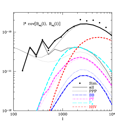
Refer to caption
Figure 5: Diagonal terms of the bispectrum covariance matrix for equilateral triangle configurations as a function of the side length l𝑙l, as in the previous figure. The covariance amplitude is shown in the unit of l6Cov[Beq(l),Beq(l)]superscript𝑙6Covsubscript𝐵eq𝑙subscript𝐵eq𝑙l^{6}{\rm Cov}[B_{\rm eq}(l),B_{\rm eq}(l)], since l3Beq(l)superscript𝑙3subscript𝐵eq𝑙l^{3}B_{\rm eq}(l) gives the contribution to the skewness κ3delimited-⟨⟩superscript𝜅3\left\langle{\kappa^{3}}\right\rangle. The points are the simulation results estimated from the scatters of 1000 simulations. The other curves are the halo model predictions, which are computed based on the method described in Section 3.2. The dotted, long dot–dashed, short dot–dashed, and long dashed curves are the contributions that are proportional to P3,B2,PTsuperscript𝑃3superscript𝐵2𝑃𝑇P^{3},B^{2},PT and P6subscript𝑃6P_{6}, respectively (also see Fig. 1). For thick curves, we used the power spectra P(l)𝑃𝑙P(l), the bispectra B(l)𝐵𝑙B(l) and the number of triangles directly estimated from the simulations. For comparison, the thin curves show the results if we use the halo model for P(l)𝑃𝑙P(l) and B(l)𝐵𝑙B(l) as well as equation (16) for the number of triangles. The short dashed curve is the HSV contribution, which dominates over other terms at multipole bins, l2000greater-than-or-similar-to𝑙2000l\ga 2000. The solid curves are the total contribution, the sum of all the terms.
Refer to caption
Refer to caption
Figure 6: Similar to the previous plot, but for different triangle configurations. Left-hand panels: the covariance matrix for isosceles triangle configurations, B(l1,l2,l3)𝐵subscript𝑙1subscript𝑙2subscript𝑙3B(l_{1},l_{2},l_{3}), with l1=l2subscript𝑙1subscript𝑙2l_{1}=l_{2}. The different panels are for different side lengths l1subscript𝑙1l_{1} and l2subscript𝑙2l_{2}; within each panel, the covariance matrix is shown as a function of l3subscript𝑙3l_{3}. Note that the covariance matrix is shown in the multipole range where the triangle conditions |ljlk|lilj+lksubscript𝑙𝑗subscript𝑙𝑘subscript𝑙𝑖subscript𝑙𝑗subscript𝑙𝑘|l_{j}-l_{k}|\leq l_{i}\leq l_{j}+l_{k} are satisfied, but the condition l1l2l3subscript𝑙1subscript𝑙2subscript𝑙3l_{1}\leq l_{2}\leq l_{3} is not imposed. Right-hand panels: the covariance matrix elements between the bispectra of isosceles and equilateral triangles. The Gaussian terms of P3superscript𝑃3P^{3} denoted by the vertical dotted lines appear at a particular value of l3subscript𝑙3l_{3}, where the two triangles become the same, i.e. equilateral triangles with l1=l2=l3subscript𝑙1subscript𝑙2subscript𝑙3l_{1}=l_{2}=l_{3}.
Refer to caption
Figure 7: Cross-covariance between the power spectrum and the bispectrum of equilateral triangles, Cov[P(l),Beq(l)]Cov𝑃𝑙subscript𝐵eq𝑙{\rm Cov}[P(l),B_{\rm eq}(l)], as a function of l𝑙l. The covariance amplitude is plotted in the units of l5Cov[P,Beq]superscript𝑙5Cov𝑃subscript𝐵eql^{5}{\rm Cov}[P,B_{\rm eq}], because l2Psuperscript𝑙2𝑃l^{2}P and l3Bsuperscript𝑙3𝐵l^{3}B contribute to κ2delimited-⟨⟩superscript𝜅2\left\langle{\kappa^{2}}\right\rangle and κ3delimited-⟨⟩superscript𝜅3\left\langle{\kappa^{3}}\right\rangle, respectively. Note that there is no Gaussian error contribution to the cross-covariance, because it arises from the five-point correlation functions. The different curves are the model predictions that are computed based on the method in Section 3.3.
Refer to caption
Figure 8: Correlation coefficients rijXYsubscriptsuperscript𝑟𝑋𝑌𝑖𝑗r^{XY}_{ij} (defined by equation 25) for the power spectrum and bispectrum covariance and the cross-covariance between the power spectrum and the bispectrum, where X,Y=P𝑋𝑌𝑃X,Y=P or B𝐵B and the indices i𝑖i or j𝑗j denote the multipole bin or the triangle configuration, e.g. Xi=B(𝒍i)subscript𝑋𝑖𝐵subscript𝒍𝑖X_{i}=B(\mbox{\boldmath$l$}_{i}). Note that the diagonal elements riiXX=1subscriptsuperscript𝑟𝑋𝑋𝑖𝑖1r^{XX}_{ii}=1 by definition. The upper-right matrix elements show the simulation results, while the lower-left elements show the halo model predictions with the HSV effect. The upper-left square-shaped panel (16×16161616\times 16 elements) shows riPPjsubscriptsuperscript𝑟𝑃𝑃𝑖𝑗r^{PP}_{i}j for the power spectrum covariance. The lower-right panel (204×204204204204\times 204) shows the bispectrum covariance matrix rijBBsubscriptsuperscript𝑟𝐵𝐵𝑖𝑗r^{BB}_{ij}. The upper-right or lower-left rectangular-shape panels (16×2041620416\times 204 or 204×1620416204\times 16) show the cross-covariance matrix rijPBsubscriptsuperscript𝑟𝑃𝐵𝑖𝑗r^{PB}_{ij} or rijBPsubscriptsuperscript𝑟𝐵𝑃𝑖𝑗r^{BP}_{ij}. As the multipole becomes larger, the correlation coefficients have larger values and approach rijXY1similar-to-or-equalssuperscriptsubscript𝑟𝑖𝑗𝑋𝑌1r_{ij}^{XY}\simeq 1.
Refer to caption
Figure 9: Similar plot to the previous figure, but the halo model predictions without the HSV effect are shown (the lower-left matrix elements). Note that the simulation results (the upper-right elements) are the same as in the previous figure. It is evident that the halo model predictions are well below the simulation measurements for large multipoles owing to the missing HSV terms.

In Figs 57, we study the covariance matrices of the lensing bispectra for some representative triangle configurations of the 204 triangles. Note that, in these results, the two triangle configurations of the covariance have the same length(s) for at least one side length (e.g. l1=l1subscript𝑙1superscriptsubscript𝑙1l_{1}=l_{1}^{\prime}). Hence the covariance terms O(BB)𝑂𝐵𝐵O(BB) and O(PT)𝑂𝑃𝑇O(PT) in Fig. 1 are not vanishing for the covariances shown in these figures. First, in Fig. 5, we study the diagonal terms of the bispectrum covariance matrix for equilateral triangles, Cov[Beq(l),Beq(l)]Covsubscript𝐵eq𝑙subscript𝐵eq𝑙{\rm Cov}[B_{\rm eq}(l),B_{\rm eq}(l)], as a function of the side length l𝑙l. The points are the simulation results. The jagged feature at small l𝑙l bins is due to the effect of discrete pixels in the lensing maps. The different curves are the halo model predictions for the covariance matrix (equations 18 and 19). The dotted curve shows the Gaussian error contribution that scales with P(l)3𝑃superscript𝑙3P(l)^{3}, where we use the number of triangles directly computed from the simulated lensing map. The long dot–dashed, short dot–dashed, long dashed and short dashed curves are the different non-Gaussian terms. For these calculations, we use the P(l)𝑃𝑙P(l) and Beq(l)subscript𝐵eq𝑙B_{\rm eq}(l) directly estimated from the 1000 ray-tracing simulations, while we use the halo model in Section 3.5 to compute the the higher-order functions. The solid curve is the total power of the covariance matrix, the sum of the terms above. The figure clearly shows that the non-Gaussian errors become significant at la few 100greater-than-or-similar-to𝑙a few 100l\ga\mbox{a few }100, and the model predictions are in good agreement with the simulation results if we include the HSV term. The HSV term dominates the other terms at l1000greater-than-or-similar-to𝑙1000l\ga 1000. These findings are similar to the results in the power spectrum covariance (see figs 5–7 in Sato et al. 2009).

Fig. 6 shows the covariance matrices for isosceles triangle configurations (left panel) and the off-diagonal components between different triangle configurations, equilateral and isosceles triangles (right panel). For this plot, we do not use the condition l1l2l3subscript𝑙1subscript𝑙2subscript𝑙3l_{1}\leq l_{2}\leq l_{3} for presentation purposes, but all the triangles shown here are indeed included in the covariance matrix elements we will use in the following analysis. Even for these more general triangle configurations, the model predictions including the HSV effect are in good agreement with the simulations. One may find that the covariance amplitudes or some non-Gaussian terms peak at some particular value of l3subscript𝑙3l_{3} in the x𝑥x-axis. This happens when the isosceles triangles have higher symmetry, equilateral shape; the number of independent triangles is smaller for higher-symmetry triangles, leading to the greater covariance amplitudes.

In Fig. 7, we study the cross-covariance between the power spectrum and the bispectrum of equilateral triangles, Cov[P(l),Beq(l)]Cov𝑃𝑙subscript𝐵eq𝑙{\rm Cov}[P(l),B_{\rm eq}(l)], as a function of the multipole bin l𝑙l. There is no Gaussian error contribution because the cross-covariance arises from the five-point functions. The figure again shows that the model predictions including the HSV term well reproduces the simulation results.

In Fig. 8, we compare the halo model predictions with the simulation results for all the matrix elements of the power spectrum covariance, the bispectrum covariance and the cross-covariance, in one figure. To do this, we use the correlation coefficients of the covariance matrices defined as

rijXYCov[Xi,Yj]Cov[Xi,Xi]Cov[Yj,Yj],subscriptsuperscript𝑟𝑋𝑌𝑖𝑗Covsubscript𝑋𝑖subscript𝑌𝑗Covsubscript𝑋𝑖subscript𝑋𝑖Covsubscript𝑌𝑗subscript𝑌𝑗r^{XY}_{ij}\equiv\frac{{\rm Cov}[X_{i},Y_{j}]}{\sqrt{{\rm Cov}[X_{i},X_{i}]{\rm Cov}[Y_{j},Y_{j}]}}, (25)

where X𝑋X and Y𝑌Y are the power spectrum or the bispectrum, and the subscript i𝑖i or j𝑗j in X𝑋X or Y𝑌Y denote the i𝑖ith multipole bin or the i𝑖ith triangle configuration; Xi=P(li),Xi=B(𝒍i)formulae-sequencesubscript𝑋𝑖𝑃subscript𝑙𝑖subscript𝑋𝑖𝐵subscript𝒍𝑖X_{i}=P(l_{i}),X_{i}=B(\mbox{\boldmath$l$}_{i}), and so on. The diagonal components rii=1subscript𝑟𝑖𝑖1r_{ii}=1 by definition. If rij=0subscript𝑟𝑖𝑗0r_{ij}=0, it means no correlation between the spectra Xisubscript𝑋𝑖X_{i} and Yjsubscript𝑌𝑗Y_{j}, while the the higher values of rijsubscript𝑟𝑖𝑗r_{ij} mean stronger correlations. For illustration purposes, we use the following indices of the 204 triangles so that the different triangles are indexed in increasing order of l3subscript𝑙3l_{3}:

Δ(il1,il2,il3)Δsubscript𝑖subscript𝑙1subscript𝑖subscript𝑙2subscript𝑖subscript𝑙3\displaystyle\Delta(i_{l_{1}},i_{l_{2}},i_{l_{3}}) =\displaystyle= (1,1,1),111\displaystyle(1,1,1), (26)
(1,1,2),(1,2,2),(2,2,2),112122222\displaystyle(1,1,2),(1,2,2),(2,2,2),
(1,1,3),(1,2,3),(1,3,3),(2,2,3),(2,3,3),(3,3,3),113123133223233333\displaystyle(1,1,3),(1,2,3),(1,3,3),(2,2,3),(2,3,3),(3,3,3),
(1,3,4),,134\displaystyle(1,3,4),\cdots,
\displaystyle\vdots
(1,16,16),,(14,14,16),(14,15,16),(14,16,16),(15,15,16),(15,16,16),(16,16,16),11616141416141516141616151516151616161616\displaystyle(1,16,16),\cdots,(14,14,16),(14,15,16),(14,16,16),(15,15,16),(15,16,16),(16,16,16),

where we have used the 16 logarithmically spaced multipole bins of l𝑙l. Note that, for a given l3subscript𝑙3l_{3}-bin, the other multipole bins (l1,l2)subscript𝑙1subscript𝑙2(l_{1},l_{2}) are listed in increasing order of l1subscript𝑙1l_{1} (l1l2subscript𝑙1subscript𝑙2l_{1}\leq l_{2} for each triangle index). With this triangle index, the higher-index triangle configuration corresponds to the triangles having higher multipoles or larger side lengths. The figure shows that the halo model well reproduces the two-dimensional features of the covariance matrices seen from the simulations.101010 In Fig. 8 we fully used the halo model to compute the covariance matrix elements including the power spectrum and bispectrum, unlike in Figs 57. Most of the off-diagonal terms of the bispectrum covariance consist of only the term O(P6)𝑂subscript𝑃6O(P_{6}) and the HSV term, because in general the shapes of two triangles are different from each other in contrary to the cases of Figs 5 and 6. The correlation coefficients become greater at higher multipoles, almost rij1similar-to-or-equalssubscript𝑟𝑖𝑗1r_{ij}\simeq 1. For comparison, Fig. 9 shows the results without the HSV term in the halo model predictions (the simulation results are the same to the previous figure), where the discrepancy is clear.

4.4 Information content of the lensing bispectrum

As we have studied, the non-linear structure formation induces non-Gaussian errors in the weak lensing field, provoking significant correlations between the power spectra of different multipoles and the bispectra of different triangle configurations as well as significant cross-correlations between the power spectra and the bispectra. Then a more fundamental, important question arises. How much additional information do the lensing bispectra carry to the lensing power spectrum? Can joint measurements of the power spectra and bispectra recover the information content of the Gaussian field, which the primordial density field of structure formation should have had as in the CMB case? In this section, we address these questions.

A useful quantity to quantify the impact of the non-Gaussian errors is the expected signal-to-noise ratio (S/N) for a measurement of the lensing power spectra and bispectra in a given survey that is characterized by its area and shot noise parameters. The S/N is sometimes called the information content (Tegmark et al. 1997) (also see Takada & Jain 2009, and references therein). For the power spectrum measurement, the S/N is defined as

(SN)P2li,lj<lmaxP(li)[𝑪P]ij1P(lj),superscriptsubscript𝑆𝑁𝑃2subscriptsubscript𝑙𝑖subscript𝑙𝑗subscript𝑙max𝑃subscript𝑙𝑖subscriptsuperscriptdelimited-[]superscript𝑪𝑃1𝑖𝑗𝑃subscript𝑙𝑗\left(\frac{S}{N}\right)_{P}^{2}\equiv\sum_{l_{i},l_{j}<l_{\rm max}}P(l_{i})\left[\mbox{\boldmath$C$}^{P}\right]^{-1}_{ij}P(l_{j}), (27)

where the summation indices i,j𝑖𝑗i,j run over multipole bin indices up to a given maximum multipole lmaxsubscript𝑙maxl_{\rm max}, and [𝑪P]1superscriptdelimited-[]superscript𝑪𝑃1[\mbox{\boldmath$C$}^{P}]^{-1} is the inverse of the power spectrum covariance matrix. The inverse of S/N is equivalent to a precision of measuring the logarithmic amplitude of the power spectrum up to a given maximum multipole lmaxsubscript𝑙maxl_{\rm max}, assuming that the shape of the power spectrum is perfectly known. The S/N is independent of the multipole bin width as long as the bin width is fine enough to capture the shape of the lensing power spectrum (on the other hand, the relative strength of the non-Gaussian errors to the Gaussian errors depends on the width). Similarly, the S/N for the bispectrum measurement or the information content about the bispectrum amplitude is defined as

(SN)B2={li},{lj}lmaxBi[𝑪B]ij1Bj,superscriptsubscript𝑆𝑁𝐵2subscriptsubscript𝑙𝑖subscript𝑙𝑗subscript𝑙maxsubscript𝐵𝑖subscriptsuperscriptdelimited-[]superscript𝑪𝐵1𝑖𝑗subscript𝐵𝑗\left(\frac{S}{N}\right)_{B}^{2}=\sum_{\{l_{i}\},\{l_{j}\}\leq l_{\rm max}}B_{i}\left[\mbox{\boldmath$C$}^{B}\right]^{-1}_{ij}B_{j}, (28)

where the summation indices i,j𝑖𝑗i,j run over triangle configurations, and we include all the triangle configurations whose side lengths are smaller than a given maximum multipole lmaxsubscript𝑙maxl_{\rm max}.

We also consider the S/N for a combined measurement of the lensing power spectra and bispectra up to a given lmaxsubscript𝑙maxl_{\rm max}. In the presence of the non-Gaussian errors, the total S/N is not simply a sum of the two estimates of S/N of the power spectra and the bispectra due to the cross-covariance. To study this, we first define the data vector for the joint measurement as

𝑫={P1,P2,,Pnb,B1,B2,,Bitriang,max}.𝑫subscript𝑃1subscript𝑃2subscript𝑃subscript𝑛𝑏subscript𝐵1subscript𝐵2subscript𝐵subscript𝑖triangmax\mbox{\boldmath$D$}=\left\{P_{1},P_{2},\cdots,P_{n_{b}},B_{1},B_{2},\cdots,B_{i_{\rm triang,max}}\right\}. (29)

The covariance matrix for the data vector 𝑫𝑫D is given as

𝑪P+B=(𝑪P𝑪PB𝑪PB𝑪B),superscript𝑪𝑃𝐵superscript𝑪𝑃superscript𝑪𝑃𝐵superscript𝑪𝑃𝐵superscript𝑪𝐵{\mbox{\boldmath$C$}}^{P+B}=\left(\begin{array}[]{cc}\mbox{\boldmath$C$}^{P}&\mbox{\boldmath$C$}^{PB}\\ \mbox{\boldmath$C$}^{PB}&\mbox{\boldmath$C$}^{B}\end{array}\right), (30)

where the 𝑪PBsuperscript𝑪𝑃𝐵\mbox{\boldmath$C$}^{PB} is the cross-covariance between the power spectrum and the bispectrum. Then, the total (S/N)P+B is similarly defined as

(SN)P+B2=i,jlmaxDi[𝑪P+B]ij1Dj.subscriptsuperscript𝑆𝑁2𝑃𝐵subscript𝑖𝑗subscript𝑙maxsubscript𝐷𝑖subscriptsuperscriptdelimited-[]superscript𝑪𝑃𝐵1𝑖𝑗subscript𝐷𝑗\left(\frac{S}{N}\right)^{2}_{P+B}=\sum_{i,j\leq l_{\rm max}}D_{i}\left[\mbox{\boldmath$C$}^{P+B}\right]^{-1}_{ij}D_{j}. (31)
Refer to caption
Figure 10: Cumulative S/N for the power spectrum (P𝑃P), the bispectrum (B𝐵B) and the joint measurement (P+B𝑃𝐵P+B) for a survey area of 25 deg2 and source redshift zs=1subscript𝑧𝑠1z_{s}=1. They are shown as functions of the maximum multipole lmaxsubscript𝑙maxl_{\rm max}, where the power spectrum and/or bispectrum information are included over lminllmaxsubscript𝑙min𝑙subscript𝑙maxl_{\rm min}\leq l\leq l_{\rm max} (see equations 27, 28 and 31). The minimum multipole is set to lmin=72subscript𝑙min72l_{\rm min}=72. We do not include the shape noise contamination here – it is shown in the next figure. The circle, triangle and square symbols are the simulation results for P𝑃P, B𝐵B and P+B𝑃𝐵P+B measurements, respectively, computed from the 1000 realizations. The thick short-dashed, long-dashed and solid curves are the corresponding halo model predictions. The corresponding thin curves are the results without the HSV contributions. For comparison, the dotted curve shows the S/N for the power spectrum for the Gaussian field, which the primordial density field should have contained. Note that the simulation results for B𝐵B and P+B𝑃𝐵P+B could be overestimated by about 10 per cent due to a finite number of the simulation realizations used to estimate the covariance matrices (Hartlap et al. 2007).

Fig. 10 shows the expected S/N for measurements of the power spectra and the bispectra for a survey area of 25 square degrees (i.e. the area of the ray-tracing simulation), as a function of the maximum multipole lmaxsubscript𝑙maxl_{\rm max} up to which the power spectrum and/or bispectrum information are included. The minimum multipole is fixed to lmin=72subscript𝑙min72l_{\rm min}=72. We do not include the shot noise contamination to the error covariance matrices, so the results solely correspond to the cosmological information contents. The circle, triangle and square symbols are the simulation results for the S/N of the power spectra, the bispectra and the joint measurements, respectively, which are computed using the 1000 realizations. The thick/thin short-dashed, long-dashed and solid curves are the halo model predictions with/without the HSV terms. First of all, the lensing bispectra add new information content to the power spectrum measurement. To be more quantitative, adding the bispectrum measurement increases the S/N by about 50 per cent for lmax103similar-to-or-equalssubscript𝑙maxsuperscript103l_{\rm max}\simeq 10^{3} compared to the power spectrum measurement alone. Note that the lmaxsubscript𝑙maxl_{\rm max} of a few thousands is the typical maximum multipole for upcoming weak lens surveys. This improvement is equivalent to about 2.3 larger survey area for the power spectrum measurement alone; that is, the same data sets can be used to obtain the additional information, if the bispectrum measurement is combined with the power spectrum measurement. Secondly, the halo model predictions are in nice agreement with the simulation results. Note that the total S/N for the joint measurement (P+B𝑃𝐵P+B) is close to the linear sum of the S/N values ((S/N)P and (S/N)B), not the sum of their squared values (S/N)2, due to the significant cross-covariance between P𝑃P and B𝐵B (see Appendix C in Takada & Bridle 2007, for the similar discussion). If ignoring the cross-covariance, adding the bispectrum measurement does not much improve the S/N (only by 5 per cent or so). Hence it is important to take into account the correlation between the two measurements.

Next, let us compare the result above with the case of a Gaussian random field, which is shown in the dashed curve in Fig. 10. The S/N for a Gaussian field is equivalent to the number of independent Fourier modes up to a lmaxsubscript𝑙maxl_{\rm max} for a given survey area. The figure clearly shows that the joint measurement of the power spectrum and the bispectrum does not recover the full information content of the Gaussian field. This implies that the higher-order statistics beyond the bispectrum are also important to recover the full information content. One may argue that the initial memory of the field cannot be recovered due to the non-linear structure formation. However, we would like to note that, if ignoring the HSV contribution to the covariance, adding the bispectrum can recover about 75 per cent of the Gaussian information, as shown by the thin curves. Hence the loss of the information contents is mostly due to the the HSV contribution. As discussed in Section 3.4, the HSV alters the overall amplitude but preserves the shape of the lensing spectra. Hence the HSV may give the worst case degradation of the amplitude parameter, but may not cause any serious degradation of parameters that are sensitive to the shapes of the lensing spectra. A genuine impact of the HSV on cosmological parameters needs to be further studied and this is our future work.
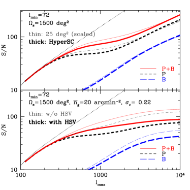
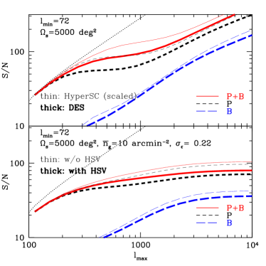
Refer to caption
Refer to caption
Figure 11: Cumulative S/N, as in the previous figure, but for upcoming weak lensing surveys, the Subaru Hyper Suprime-Cam (HyperSC) survey and the DES in the left- and right-hand panels, respectively. These surveys are characterized by survey parameters: survey area (ΩssubscriptΩs\Omega_{\rm s}), mean source redshift (z¯ssubscript¯𝑧𝑠\bar{z}_{s}), and mean (effective) number density of source galaxies (n¯gsubscript¯𝑛𝑔\bar{n}_{g}). We assumed Ωs=1500subscriptΩs1500\Omega_{\rm s}=1500 deg2, z¯s=1subscript¯𝑧𝑠1\bar{z}_{s}=1, and n¯g=20subscript¯𝑛𝑔20\bar{n}_{g}=20 arcmin-2 for the HyperSC survey and Ωs=5000subscriptΩs5000\Omega_{\rm s}=5000 deg2, z¯s=0.7subscript¯𝑧𝑠0.7\bar{z}_{s}=0.7, and n¯g=10subscript¯𝑛𝑔10\bar{n}_{g}=10 arcmin-2 for the DES. We set σϵ=0.22subscript𝜎italic-ϵ0.22\sigma_{\epsilon}=0.22 for the rms intrinsic ellipticity per component for both the surveys. The upper and lower plots in each panel show the results without and with the shot noise contamination. The thin curves in the upper plot of the left-hand panel shows the S/N values obtained by scaling the results for 252525 deg2 in Fig. 10 assuming S/N Ωs1/2proportional-toabsentsuperscriptsubscriptΩs12\propto\Omega_{\rm s}^{1/2}. The thin curves in the upper plot of the right-hand panel are similar, but obtained by scaling the HyperSC results in the left panel to 5000 deg2. The lower plots in each panel show the results including the shot noise contribution to the covariance, but the thin/thick lines are without/with the HSV terms.

Expected cumulative S/N for the upcoming weak lensing surveys

Survey Subaru HyperSC Survey DES
lmax()subscript𝑙maxsimilar-to-or-equalsl_{\rm max}(\simeq) 100010001000 100010001000 200020002000 200020002000 100010001000 100010001000 200020002000 200020002000
shot noise (σϵsubscript𝜎italic-ϵ\sigma_{\epsilon}) w/o with w/o with w/o with w/o with
(S/N)P 53 48 74 57 75 56 116 63
(S/N)B 19 16 35 26 33 20 59 29
(S/N)P+B 78 (48%) 64 (33%) 98 (32%) 72 (26%) 103 (37%) 66 (18%) 145 (25%) 73 (16%)
Table 1: Cumulative S/N of the power spectrum (P𝑃P), the bispectrum (B)𝐵(B) and the joint measurement (P+B𝑃𝐵P+B) expected for the upcoming weak lensing surveys, the Subaru Hyper Suprime-Cam survey (HyperSC) and the DES, as in Fig. 11. Here we consider lmax1000similar-to-or-equalssubscript𝑙max1000l_{\rm max}\simeq 1000 and 2000 for the maximum multipole (more exactly, the bins of lmax=1245subscript𝑙max1245l_{\rm max}=1245 and 226822682268). The column denoted by ‘w/o’ or ‘with’ in the row ‘shot noise’ gives the S/N values with and without the intrinsic shape noise contribution to the covariances. The percentage in the parenthesis shows the improvement of S/N for the joint measurement (P+B𝑃𝐵P+B) compared to the power spectrum alone (P𝑃P).

In Fig. 11 and Table 1, we show the S/N expected for the upcoming wide-field weak lensing surveys, the Subaru Hyper Suprime-Cam (HyperSC) survey and the DES, which are characterized by the survey area, the mean source redshift and the mean number density of source galaxies of Ωs=1500subscriptΩs1500\Omega_{\rm s}=1500 sq. degrees, z¯s=1subscript¯𝑧𝑠1\bar{z}_{s}=1 and n¯g=20subscript¯𝑛𝑔20\bar{n}_{g}=20 arcmin-2 for the HyperSC survey, while Ωs=5000subscriptΩs5000\Omega_{\rm s}=5000 deg2, z¯s=0.7subscript¯𝑧𝑠0.7\bar{z}_{s}=0.7 and n¯g=10subscript¯𝑛𝑔10\bar{n}_{g}=10 arcmin-2 for the DES, respectively. Here we employ the halo model to compute the S/N and assume a circular survey geometry for simplicity. The figure and table show that these surveys promise a significant detection of the lensing bispectrum; (S/N) 26similar-to-or-equalsabsent26\simeq 26 or 292929 for the HyperSC or the DES, respectively, when assuming lmax2000similar-to-or-equalssubscript𝑙max2000l_{\rm max}\simeq 2000 and including the shot noise effect. It also means that the theoretical prediction of the lensing bispectrum needs to be as accurate as a few per cent for the upcoming surveys. We find that the bispectrum adds new information, increasing the total S/N by about 20 – 30 per cent compared to the power spectrum alone, which is equivalent to a factor of 1.4 – 1.7 larger survey area.

Fig. 11 also shows that the HSV is significant for these surveys. The thin curves in the upper plots of the left-panel are the S/N computed by scaling the values for 25 deg2 in Fig. 10 assuming S/N Ωs1/2proportional-toabsentsuperscriptsubscriptΩs12\propto\Omega_{\rm s}^{1/2}. Since the covariance terms except for the HSV term scale as 1/Ωs1subscriptΩs1/\Omega_{\rm s}, the differences between the thick and thin curves are due to the HSV term which depends on the survey area via the shape of the matter power spectrum convolved with the survey window function (see the discussion below equation 14). The S/N values are smaller than the naively-scaled results, which means that the HSV decreases more slowly than 1/Ωs1subscriptΩs1/\Omega_{\rm s}. The upper plot of the right panel shows the similar plot, but for the DES results with scaled values for the HyperSC in the left panel. The S/N are smaller than the scaled HyperSC results, because the typical source redshift of z¯s=0.7subscript¯𝑧𝑠0.7\bar{z}_{s}=0.7 for the DES is lower than that of the HyperSC of z¯s=1subscript¯𝑧𝑠1\bar{z}_{s}=1 and the DES is more sensitive to the non-linear density fluctuations. The HSV has significant influence on the S/N even in the presence of the shot noise as shown in the lower panels of the figure. Although the shot noise leads to a saturation of the S/N at large multipoles, note that the systematic effects such as the highly non-linear clustering effect and/or the baryonic effect become more significant at these high multipoles (White 2004; Zhan & Knox 2004; Huterer & Takada 2005; Huterer et al. 2006).

4.5 Principal component analysis of the lensing covariance matrices

A principal component analysis (PCA) of the power spectrum and bispectrum covariance matrices is useful to quantify how the different power spectra and/or bispectra are correlated with each other and how many independent modes or triangles contribute to most of the information contents (Takada & Jain 2009) (also see Scoccimarro 2000, for the the 3D bispectrum case). Since the covariance matrix is symmetric by definition, it can always be decomposed as

CijX=aSaiX(λaX)2SajX,subscriptsuperscript𝐶𝑋𝑖𝑗subscript𝑎subscriptsuperscript𝑆𝑋𝑎𝑖superscriptsubscriptsuperscript𝜆𝑋𝑎2subscriptsuperscript𝑆𝑋𝑎𝑗C^{X}_{ij}=\sum_{a}S^{X}_{ai}(\lambda^{X}_{a})^{2}S^{X}_{aj}, (32)

where X𝑋X is the lensing power spectrum or bispectrum, λaXsuperscriptsubscript𝜆𝑎𝑋\lambda_{a}^{X} is the a𝑎ath eigenvalue or principal component, (𝑺X)1=(𝑺X)Tsuperscriptsuperscript𝑺𝑋1superscriptsuperscript𝑺𝑋𝑇(\mbox{\boldmath$S$}^{X})^{-1}=(\mbox{\boldmath$S$}^{X})^{T}, kSikXSjkX=δijKsubscript𝑘subscriptsuperscript𝑆𝑋𝑖𝑘subscriptsuperscript𝑆𝑋𝑗𝑘subscriptsuperscript𝛿𝐾𝑖𝑗\sum_{k}S^{X}_{ik}S^{X}_{jk}=\delta^{K}_{ij} and 𝑺Xsuperscript𝑺𝑋\mbox{\boldmath$S$}^{X} is normalized so as to satisfy j(SijX)2=1subscript𝑗superscriptsubscriptsuperscript𝑆𝑋𝑖𝑗21\sum_{j}(S^{X}_{ij})^{2}=1. The matrix SaiXsubscriptsuperscript𝑆𝑋𝑎𝑖S^{X}_{ai} is considered as the projection matrix as it describes how the power in the i𝑖ith multipole bin or triangle configuration is projected onto the a𝑎ath eigenmode. Using this representation, the inverse of the covariance matrix is given by [𝑪X]ij1=SiaX(1/λaX)2SjaXsubscriptsuperscriptdelimited-[]superscript𝑪𝑋1𝑖𝑗superscriptsubscript𝑆𝑖𝑎𝑋superscript1subscriptsuperscript𝜆𝑋𝑎2superscriptsubscript𝑆𝑗𝑎𝑋[\mbox{\boldmath$C$}^{X}]^{-1}_{ij}=S_{ia}^{X}(1/\lambda^{X}_{a})^{2}S_{ja}^{X}. Hence, the S/N values (equations 27 or 28) can be rewritten as

(SN)X2=a{1λaXiSaiXXi}2,subscriptsuperscript𝑆𝑁2𝑋subscript𝑎superscript1superscriptsubscript𝜆𝑎𝑋subscript𝑖subscriptsuperscript𝑆𝑋𝑎𝑖subscript𝑋𝑖2\left(\frac{S}{N}\right)^{2}_{X}=\sum_{a}\left\{\frac{1}{\lambda_{a}^{X}}\sum_{i}S^{X}_{ai}X_{i}\right\}^{2}, (33)

where Xisubscript𝑋𝑖X_{i} is either P(li)𝑃subscript𝑙𝑖P(l_{i}), B(𝒍i)𝐵subscript𝒍𝑖B(\mbox{\boldmath$l$}_{i}) or the joint (P+B𝑃𝐵P+B). Thus, since (1/λaX)iSaiXXi1superscriptsubscript𝜆𝑎𝑋subscript𝑖superscriptsubscript𝑆𝑎𝑖𝑋subscript𝑋𝑖(1/\lambda_{a}^{X})\sum_{i}S_{ai}^{X}X_{i} can be considered as the S/N for the a𝑎ath eigenmode, the above equation expresses the total S/N (for a given lmaxsubscript𝑙maxl_{\rm max}) as a sum of contributions from the independent eigenmodes. We can then re-order the eigenmodes such that the lower eigenmode has the higher contribution to the S/N.
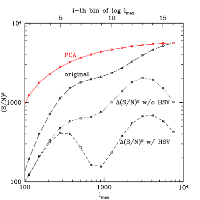
Refer to caption
Refer to caption
Figure 12: PCA of the power spectrum covariance for the 16 logarithmically spaced multipole bins over 72l8748.872𝑙8748.872\leq l\leq 8748.8, for the Subaru HyperSC-type survey with 1500 deg2 and with the shot noise. Left-hand panel: the long-dashed curve shows the cumulative (S/N)2 for the power spectrum as in the left-lower panel of Fig. 11, but for (S/N)2 instead of S/N (the points denote the central value of each multipole bin). The short-dashed and dotted curves show the differential contribution to the (S/N)2 at each multipole bin, with and without the HSV effect, respectively. The solid curve shows how the (S/N)2 value is recovered by adding the PCA eigenmodes. Note that the PCA results are shown as a function of the order of the PCA eigenmodes, where the PCA eigenmodes are ranked in decreasing order of the differential contribution to the (S/N)2 (see equation 33). Right-hand panel: the projection matrix |Sai|subscript𝑆𝑎𝑖|S_{ai}| for the first eight eigenmodes, where the index a𝑎a denotes the a𝑎ath eigenmode.

Fig. 12 shows the PCA results for the power spectrum measurement for the Subaru HyperSC-type survey including the shot noise effect as in Fig. 11. This figure can be compared with Fig. 5 in Takada & Jain (2009), where the HSV effect was not included. The short-dashed and dotted curves show each contribution of the i𝑖ith multipole bin to the total (S/N)2 with and without the HSV, respectively. It should be stressed that the power spectrum of l103similar-to𝑙superscript103l\sim 10^{3} has a local minimum, due to the significant HSV contribution.

The long-dashed curve shows the total (S/N)2 as a function of the maximum multipole lmaxsubscript𝑙maxl_{\rm max}, up to lmax=8748.8subscript𝑙max8748.8l_{\rm max}=8748.8 (the 16-th multipole bin). On the other hand, the solid curve shows how the cumulative (S/N)2 value increases by adding the a𝑎ath eigenmode (equation 33)111111First, we made the principal component analysis of the power spectrum covariance matrix including up to the multipole bin l=8748.8𝑙8748.8l=8748.8 (i.e. 16×16161616\times 16 matrix). Then, we re-ordered the eigenmodes in increasing order of the differential (S/N)2 value. The solid curve in Fig. 12 shows how the cumulative S/N value increases by adding a new a𝑎ath eigenmode.. The figure shows that, among the 16 multipole bins, including about seven eigenmodes (about half of the multipole bins) can recover about 90 per cent of the total (S/N)2. The other eigenmodes are relatively less important due to strong correlations between the different multipole bins. The right panel shows the projection matrix |Sia|subscript𝑆𝑖𝑎|S_{ia}| for each multipole bin, showing how the neighboring multipole bins are correlated with each other. The projection matrix for each eigenmode peaks at some multipole bin, but has tails to different multipole bins. In particular, the eigenmodes around a few 103superscript10310^{3} have longer tails, reflecting significant correlations between different multipole bins due to the non-Gaussian errors.
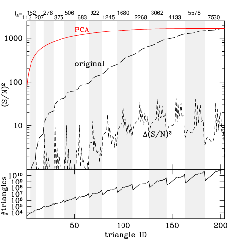
Refer to caption
Figure 13: PCA analysis of the bispectrum covariance, for the 204 triangle configurations over 72l8748.872𝑙8748.872\leq l\leq 8748.8, for the HyperSC-type survey as in the previous figure. The x𝑥x-axis denotes either the triangle index or the PCA eigenmodes. The triangle indices are in the order given by equation (26); the larger indices correspond to triangles with the larger side length of l3subscript𝑙3l_{3}. The vertical shaded regions denote the triangles with the same l3subscript𝑙3l_{3} bin, as indicated by the top label of ‘l3subscript𝑙3l_{3}’-bin values. Upper panel: the short-dashed curve shows the differential (S/N)2 of each triangle configuration, while the long dashed curve shows the cumulative (S/N)2 as in the left-lower panel of Fig. 11, but for the finer multipole bins (stepped by each triangle configuration). The solid curve shows the cumulative (S/N)2 as one adds the different PCA eigenmodes. About 70 eigenmodes out of 204 triangles can recover 90 per cent of the total (S/N)2 of the bispectrum measurement over 72l8748.872𝑙8748.872\leq l\leq 8748.8. Lower panel: the solid curve shows the number of independent triangles available from Fourier modes for the HyperSC-type survey (1500 deg2), for each triangle configuration in the x𝑥x-axis.

Fig. 13 shows the PCA analysis for the bispectrum covariance matrix, where we include the 204 triangles over 72l8748.872𝑙8748.872\leq l\leq 8748.8. The different triangle configurations contribute to the total (S/N)2 in a complex way. We use the triangle index, given by equation (26), and the higher-index triangle corresponds to triangle with larger side length of ‘l3subscript𝑙3l_{3}’, under the condition l1l2l3subscript𝑙1subscript𝑙2subscript𝑙3l_{1}\leq l_{2}\leq l_{3}. However, for a given l3subscript𝑙3l_{3} bin, either of the two side lengths l1subscript𝑙1l_{1} or l2subscript𝑙2l_{2} can be much smaller than l3subscript𝑙3l_{3}, and such a triangle configuration generally has a smaller contribution to (S/N)2. As a result, the differential (S/N)2 curve has jagged features. The sold curve shows the cumulative (S/N)2 by adding the new PCA eigenmodes, and manifests that about 70 eigenmodes, one third of the 204 triangles, carry 90 per cent of the total (S/N)2.
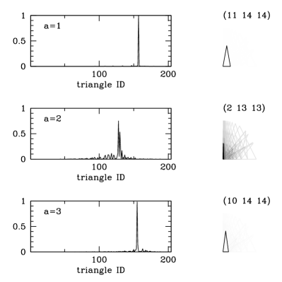
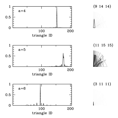
Refer to caption
Refer to caption
Figure 14: The curve in each panel shows which triangle configurations contribute to each PCA eigenmode for the bispectrum measurement in Fig. 13. We consider the first 6 PCA eigenmodes. They are labeled by the index a𝑎a from the highest contribution to the (S/N)2 and the absolute values of |Sia|subscript𝑆𝑖𝑎|S_{ia}| are plotted, where Siasubscript𝑆𝑖𝑎S_{ia} is the projection matrix of the a𝑎ath eigenfunction onto the i𝑖ith triangle configuration. The triangle configurations shown on the right side of each panel are the triangle configurations with Sia0subscript𝑆𝑖𝑎0S_{ia}\neq 0, where the triangle sizes are plotted on the linear scale and the thickness of the lines corresponds to the amplitude of |Sia|subscript𝑆𝑖𝑎|S_{ia}|. The configurations with the largest contribution are labelled in the side length bins (l1,l2,l3subscript𝑙1subscript𝑙2subscript𝑙3l_{1},l_{2},l_{3}) at top. Note that we are using logarithmically-spacing multipole bins in this paper, so about 3/4 triangles available in the Fourier space are isosceles triangles.

Fig. 14 shows which triangle configurations contribute to the first 6 PCA eigenfunctions, which therefore have the 6 highest contributions to the (S/N)2. More exactly, each panel shows the projection matrix |Sia|subscript𝑆𝑖𝑎|S_{ia}| for the a𝑎ath eigenmode (a=1,2,,6𝑎126a=1,2,\dots,6). In most panels, the projection matrix |Sia|subscript𝑆𝑖𝑎|S_{ia}| has a single or a few peaks, reflecting that the higher-S/N eigenmode arises mostly from a single or a few different triangles. For example, the highest (S/N)2 eigenfunction arises from isosceles triangles, which have side lengths of a few 103superscript10310^{3} (11- and 14-th multipole bins). However, note that we have used rather wide, logarithmically-spaced multipole bins, and most of triangle configurations available from Fourier space are close to isosceles triangle configurations. Hence, an exact shape of triangles giving a large contribution to the total (S/N)2 slightly changes with the bin width. If we take a finer multipole bin, the triangles with the highest (S/N)2 may differ from isosceles triangles.

5 Conclusion and Discussion

We have studied the covariance matrices of the lensing power spectrum and the bispectrum by using both 1000 ray-tracing simulations and the analytical halo model. We have found that there are significant non-Gaussian error contributions to the lensing covariance matrices; the power spectra or the bispectra at higher multipoles than a few hundreds are highly correlated with each other. In particular, we have shown that the mass density fluctuation at scales comparable with or outside a survey region causes significant non-Gaussian error contributions, which we call the HSV and has not been fully studied in the literature. With the HSV contributions, the halo model predictions reproduce the covariance matrices measured from the simulations (Figs 48).

Then, we have addressed how much information the lensing bispectrum adds to the power spectrum by including all the triangle configurations available up to a maximum multipole lmaxsubscript𝑙maxl_{\rm max}. Adding the bispectrum measurement improves the S/N by about 20–50 per cent compared to the power spectrum alone measurement, at lmaxsubscript𝑙maxl_{\rm max} of a few 103superscript10310^{3} (Fig. 10). We have also studied the prospects for upcoming weak lensing surveys, including the shot noise contamination due to intrinsic galaxy shapes (Fig. 11 and Table 1). The improvement in S/N is equivalent to about 1.4–2.3 larger survey area for the power spectrum measurement alone. Hence, our results show that the same imaging data can be used to improve the constraining power of cosmological parameters, if we combine the power spectrum and bispectrum measurements. We have also found that the HSV effect is significant, leading to a large degradation in the S/N. By using a PCA of the covariance matrices, we have shown that about 1/3 eigenmodes of all the triangle configurations over the range of 102l104less-than-or-similar-tosuperscript102𝑙less-than-or-similar-tosuperscript10410^{2}\la l\la 10^{4} (707070 eigenmodes compared to the 204 triangles for the multipole binning we assumed) carry most of the total information for the bispectrum measurement (Fig. 13). Thus, our results give a quantitative answer to the longstanding question of how the bispectrum can be useful and complementary to the power spectrum by fully taking into account non-Gaussian errors and all triangle configurations.

Future surveys such as the Subaru Hyper Suprime-Cam survey or the DES allow for a significant detection of the lensing bispectra (Fig. 11 and Table 1). However, there are some practical issues for making the bispectrum measurement feasible for future surveys. First, we must take into account effects of the complex survey geometry and masked regions such as saturated bright stars. This can be done by extending the method in Hikage et al. (2011) for the power spectrum measurement to the bispectrum, but has not yet been fully addressed in the literature. It is also important to explore a method of cleanly decomposing three-point correlations of E/B𝐸𝐵E/B modes in the presence of the survey window function. An alternative approach is to measure the real-space three-point correlation functions, rather than the bispectrum, which does not suffer from the geometrical problem. However, there are even more significant correlations between the three-point correlations of different triangles, and the estimate of the covariance matrices involves multi-dimensional integrations of the bispectrum covariance if one uses the halo model approach. Although the alternative to the theoretical approach may be to use a sufficient number of simulations, it will not be feasible to construct the covariance matrices for many cosmological models. Hence, which of the Fourier- or real-space is more useful/tractable for the three-point correlation measurements is still an open issue.

Although we have focused on the S/N as a measure of the information content, this is just one measure to quantify the complementarity of the lensing bispectrum. Specifically, the S/N quantifies the expected precision of the amplitude, assuming that the shapes of the power spectrum of the bispectrum are known. Hence, the S/N is not necessarily the best measure to quantify the power of the bispectrum for constraining cosmological parameters, especially parameters that are sensitive to the shape of the bispectrum (also see Takada & Jain 2009, for the similar discussion). For instance, Takada & Jain (2004) showed that the bispectrum can significantly improve the accuracy of parameter estimate from the power spectrum measurement alone, by efficiently breaking parameter degeneracies, while the S/N of the bispectrum itself is smaller than that of the power spectrum by a factor of few up to lmaxsubscript𝑙maxl_{\rm max} of a few 103superscript10310^{3} (see Fig. 5). Although they ignored the non-Gaussian error contributions to the covariances, the relative amplitude of the S/N between the power spectrum and the bispectrum is similar to our case with the full non-Gaussian terms, because the non-Gaussian terms degrade both the power spectrum and the bispectrum. Thus we can expect a similar improvement in cosmological parameters when including the bispectrum information, even with the inclusion of non-Gaussian errors. Exploring the genuine usefulness of the lensing bispectrum for cosmology is very interesting – the full forecasts for various cosmological parameters will be presented in future work.

In particular, to do such parameter forecasts, it would be much more interesting and useful if including tomographic information of the lensing field that is available from photometric redshift of source galaxies. It has been found that the lensing tomography can significantly improve the constraining power by recovering the radial-direction information of the lensing field (e.g. Takada & Jain 2004). However, for the lensing bispectrum tomography, we need to further include all the triangle configurations in different multipole and redshift bins in order to estimate the full potential. For example, if we consider three redshift bin tomography, the total number of triangles is 33×204=5508superscript3320455083^{3}\times 204=5508 for the same multipole binning as used in this paper. Thus, even 1000 realizations are not enough to reliably estimate the covariance matrices of the lensing bispectra. Hence we believe that the analytical formula we developed in this paper are essential to address these issues.

Perhaps as important as the improvement in statistical precision, the bispectrum might enable a self-calibration of systematic errors inherent in the lensing tomography measurements such as photometric redshift errors and imperfect galaxy shape measurement. Lensing bispectra depend on systematic errors in a different way from the power spectrum, but the two spectra share the same large-scale structure, hence the same cosmological parameters that describe the underlying true cosmology. Thus combining the power spectrum and bispectrum measurements can be used to self-calibrate systematic errors and improve cosmological constraints (Huterer et al. 2006). Again, it is important to fully take into account the non-Gaussian errors in order to quantify how well self-calibration works for upcoming lensing surveys.

Planned multi-colour imaging surveys can also be used to measure other cosmological probes such as the abundance of galaxy clusters and the correlation functions of galaxies. Recently, Oguri & Takada (2011) proposed a new method of using the halo–shear correlations or the stacked lensing signals around massive haloes as a function of the cluster redshifts, and showed that the stacked lensing tomography allows us to constrain cosmological measurements to a high precision. In halo (cluster)–shear correlations, the signals arise from the large-scale structure at the cluster redshift. As we have shown, massive clusters are key observables for understanding the HSV effect on the lensing power spectra. It would be interesting to pursue how the lensing power spectrum and bispectrum measurements can be combined with the cluster observables to improve cosmology parameter estimate by calibrating the HSV effect. The formulation we have developed in this paper can be straightforwardly extended to the halo–shear bispectra such as the halo–shear–shear and halo–halo–shear three-point correlation functions.

Finally, there are several effects that we have ignored in this paper and need to be studied. One is that we only considered a simple circular-shaped survey geometry to compute the HSV term. For a general geometry of the survey, the Fourier transformed survey window function becomes anisotropic and causes additional apparent correlations between the different spectra. Since the large-scale density fluctuations which contribute to the HSV are in the linear regime, it may be straightforward to take into account the effect by extending our formulation. Secondly, we have used the flat-sky approximation, which is not valid for very wide surveys such as the LSST. For a full-sky survey as the ultimate case, the HSV effect is caused by the horizon-scale perturbations with wavenumbers comparable to the matter-radiation equality wavenumber keqsubscript𝑘eqk_{\rm eq}. In this case, the HSV terms decrease more rapidly with increasing survey area than other covariance terms. Hence the HSV effect may not be that significant for such an all-sky survey. This is worth studying and the formulation and the method we developed in this paper can be used for such studies.

Acknowledgments

We would like to thank an anonymous referee for many important suggestions. We also thank Gary Bernstein, Elisabeth Krause, Takahiro Nishimichi and Masanori Sato for useful discussion. This work is supported in part by JSPS KAKENHI (Grant Number: 23340061 and 24740171), by JSPS Core-to-Core Program ‘International Research Network for Dark Energy’, by World Premier International Research Center Initiative (WPI Initiative), MEXT, Japan, by the FIRST program ‘Subaru Measurements of Images and Redshifts (SuMIRe)’, CSTP, Japan, and by NSF grant AST-0908027 and DOE grant DE-FG02-95ER40893.

References

  • Bartelmann & Schneider (2001) Bartelmann M., Schneider P., 2001, Phys. Rep., 340, 291
  • Bergé et al. (2010) Bergé J., Amara A., Réfrégier A., 2010, ApJ, 712, 992
  • Bernardeau et al. (2002) Bernardeau F., Mellier Y., van Waerbeke L., 2002, A&A, 389, L28
  • Bernardeau et al. (1997) Bernardeau F., van Waerbeke L., Mellier Y., 1997, A&A, 322, 1
  • Cooray & Hu (2001a) Cooray A., Hu W., 2001a, ApJ, 554, 56
  • Cooray & Hu (2001b) Cooray A., Hu W., 2001b, ApJ, 548, 7
  • Cooray & Sheth (2002) Cooray A., Sheth R., 2002, Physics Report, 372, 1
  • de Putter et al. (2012) de Putter R., Wagner C., Mena O., Verde L., Percival W. J., 2012, JCAP, 4, 19
  • Dodelson & Zhang (2005) Dodelson S., Zhang P., 2005, Phys. Rev. D, 72, 083001
  • Hamana & Mellier (2001) Hamana T., Mellier Y., 2001, MNRAS, 327, 169
  • Hamana et al. (2003) Hamana T. et al., 2003, ApJ, 597, 98
  • Hamilton et al. (2006) Hamilton A. J. S., Rimes C. D., Scoccimarro R., 2006, MNRAS, 371, 1188
  • Hartlap et al. (2007) Hartlap J., Simon P., Schneider P., 2007, A&A, 464, 399
  • Hikage et al. (2011) Hikage C., Takada M., Hamana T., Spergel D., 2011, MNRAS, 412, 65
  • Hoekstra & Jain (2008) Hoekstra H., Jain B., 2008, Annual Review of Nuclear and Particle Science, 58, 99
  • Hu & Kravtsov (2003) Hu W., Kravtsov A. V., 2003, ApJ, 584, 702
  • Hui (1999) Hui L., 1999, ApJ, 519, L9
  • Huterer & Takada (2005) Huterer D., Takada M., 2005, Astroparticle Physics, 23, 369
  • Huterer et al. (2006) Huterer D., Takada M., Bernstein G., Jain B., 2006, MNRAS, 366, 101
  • Jain & Khoury (2010) Jain B., Khoury J., 2010, Annals of Physics, 325, 1479
  • Jain & Seljak (1997) Jain B., Seljak U., 1997, ApJ, 484, 560
  • Jain et al. (2000) Jain B., Seljak U., White S., 2000, ApJ, 530, 547
  • Jarvis et al. (2004) Jarvis M., Bernstein G., Jain B., 2004, MNRAS, 352, 338
  • Joachimi et al. (2009) Joachimi B., Shi X., Schneider P., 2009, A&A, 508, 1193
  • Kilbinger & Schneider (2005) Kilbinger M., Schneider P., 2005, A&A, 442, 69
  • Knox (1995) Knox L., 1995, Phys. Rev. D, 52, 4307
  • Komatsu et al. (2011) Komatsu E. et al., 2011, ApJS, 192, 18
  • Lee & Pen (2008) Lee J., Pen U.-L., 2008, ApJ, 686, L1
  • Lewis et al. (2000) Lewis A., Challinor A., Lasenby A., 2000, ApJ, 538, 473
  • Limber (1954) Limber D. N., 1954, ApJ, 119, 655
  • Ma & Fry (2000) Ma C., Fry J. N., 2000, ApJ, 543, 503
  • Martin et al. (2012) Martin S., Schneider P., Simon P., 2012, A&A, 540, A9
  • Miyazaki et al. (2006) Miyazaki S. et al., 2006, in Society of Photo-Optical Instrumentation Engineers (SPIE) Conference Series.
  • Mo & White (1996) Mo H. J., White S. D. M., 1996, MNRAS, 282, 347
  • Munshi et al. (2011) Munshi D., Kitching T., Heavens A., Coles P., 2011, MNRAS, 416, 1629
  • Navarro et al. (1997) Navarro J. F., Frenk C. S., White S. D. M., 1997, ApJ, 490, 493
  • Neyrinck et al. (2009) Neyrinck M. C., Szapudi I., Szalay A. S., 2009, ApJ, 698, L90
  • Oguri & Takada (2011) Oguri M., Takada M., 2011, Phys. Rev. D, 83, 023008
  • Peacock & Smith (2000) Peacock J. A., Smith R. E., 2000, MNRAS, 318, 1144
  • Pires et al. (2012) Pires S., Leonard A., Starck J.-L., 2012, MNRAS, 423, 983
  • Rimes & Hamilton (2005) Rimes C. D., Hamilton A. J. S., 2005, MNRAS, 360, L82
  • Sato et al. (2009) Sato M., Hamana T., Takahashi R., Takada M., Yoshida N., Matsubara T., Sugiyama N., 2009, ApJ, 701, 945
  • Schneider (2006) Schneider P., 2006, in Meylan G., Jetzer P., North P., Schneider P., Kochanek C. S., Wambsganss J., eds, Saas-Fee Advanced Course 33: Gravitational Lensing: Strong, Weak and Micro. pp 269–451
  • Schrabback et al. (2010) Schrabback T. et al., 2010, A&A, 516, A63
  • Scoccimarro (2000) Scoccimarro R., 2000, ApJ, 544, 597
  • Scoccimarro & Frieman (1999) Scoccimarro R., Frieman J. A., 1999, ApJ, 520, 35
  • Scoccimarro et al. (2001) Scoccimarro R., Sheth R. K., Hui L., Jain B., 2001, ApJ, 546, 20
  • Scoccimarro et al. (1999) Scoccimarro R., Zaldarriaga M., Hui L., 1999, ApJ, 527, 1
  • Sefusatti et al. (2006) Sefusatti E., Crocce M., Pueblas S., Scoccimarro R., 2006, Phys. Rev. D, 74, 023522
  • Seljak (2000) Seljak U., 2000, MNRAS, 318, 203
  • Semboloni et al. (2008) Semboloni E., Heymans C., van Waerbeke L., Schneider P., 2008, MNRAS, 388, 991
  • Semboloni et al. (2011) Semboloni E., Schrabback T., van Waerbeke L., Vafaei S., Hartlap J., Hilbert S., 2011, MNRAS, 410, 143
  • Seo et al. (2011) Seo H.-J., Sato M., Dodelson S., Jain B., Takada M., 2011, ApJ, 729, L11
  • Shaw et al. (2009) Shaw L. D., Zahn O., Holder G. P., Doré O., 2009, ApJ, 702, 368
  • Sheth et al. (2001) Sheth R. K., Mo H. J., Tormen G., 2001, MNRAS, 323, 1
  • Smith et al. (2003) Smith R. E. et al., 2003, MNRAS, 341, 1311
  • Springel et al. (2006) Springel V., Frenk C. S., White S. D. M., 2006, Nature, 440, 1137
  • Takada & Bridle (2007) Takada M., Bridle S., 2007, New Journal of Physics, 9, 446
  • Takada & Jain (2002) Takada M., Jain B., 2002, MNRAS, 337, 875
  • Takada & Jain (2003a) Takada M., Jain B., 2003a, MNRAS, 340, 580
  • Takada & Jain (2003b) Takada M., Jain B., 2003b, MNRAS, 344, 857
  • Takada & Jain (2004) Takada M., Jain B., 2004, MNRAS, 348, 897
  • Takada & Jain (2009) Takada M., Jain B., 2009, MNRAS, 395, 2065
  • Takahashi et al. (2011) Takahashi R. et al., 2011, ApJ, 726, 7
  • Takahashi et al. (2009) Takahashi R. et al., 2009, ApJ, 700, 479
  • Tegmark et al. (1997) Tegmark M., Taylor A. N., Heavens A. F., 1997, ApJ, 480, 22
  • Valageas & Nishimichi (2011a) Valageas P., Nishimichi T., 2011a, A&A, 527, A87
  • Valageas & Nishimichi (2011b) Valageas P., Nishimichi T., 2011b, A&A, 532, A4
  • Valageas et al. (2012) Valageas P., Sato M., Nishimichi T., 2012, A&A, 541, A161
  • Van Waerbeke et al. (2001) Van Waerbeke L., Hamana T., Scoccimarro R., Colombi S., Bernardeau F., 2001, MNRAS, 322, 918
  • White (2004) White M., 2004, Astroparticle Physics, 22, 211
  • White & Hu (2000) White M., Hu W., 2000, ApJ, 537, 1
  • Zhan & Knox (2004) Zhan H., Knox L., 2004, ApJ, 616, L75
  • Zhang & Sheth (2007) Zhang P., Sheth R. K., 2007, ApJ, 671, 14
  • Zhang et al. (2003) Zhang T.-J., Pen U.-L., Zhang P., Dubinski J., 2003, ApJ, 598, 818

Appendix A Derivation of the bispectrum covariance

We derive equations of the bispectrum covariance matrix given in terms of the lensing spectra (power spectrum, bispectrum and the higher-order functions), following the method developed in Takada & Bridle (2007).

A.1 Discrete Fourier decomposition

The lensing power spectrum is estimated from the Fourier transform of the lensing convergence field, κ~𝒍subscript~𝜅𝒍\mbox{$\tilde{\kappa}$}_{\mbox{\boldmath$l$}}. When the Fourier decomposition is done in a finite survey region, the Fourier modes are by nature discrete and the fundamental mode is limited by the size of the survey area, lf=2π/Θssubscript𝑙𝑓2𝜋subscriptΘsl_{f}=2\pi/\Theta_{\rm s}, where the survey area is given by Ωs=Θs2subscriptΩssuperscriptsubscriptΘs2\Omega_{\rm s}=\Theta_{\rm s}^{2} (we assume a square survey geometry). For this case, the convergence field can be expanded using the discrete Fourier decomposition as

κ(𝜽)=1Ωs𝒍κ~𝒍ei𝒍𝜽,𝜅𝜽1subscriptΩssubscript𝒍subscript~𝜅𝒍superscript𝑒𝑖𝒍𝜽\kappa(\mbox{\boldmath$\theta$})=\frac{1}{\Omega_{\rm s}}\sum_{\mbox{\boldmath$l$}}\mbox{$\tilde{\kappa}$}_{\mbox{\boldmath$l$}}e^{i\mbox{\boldmath$l$}\cdot\mbox{\boldmath$\theta$}}, (34)

where the summation runs over the combination of integers (nx,ny)subscript𝑛𝑥subscript𝑛𝑦(n_{x},n_{y}) for 𝒍=(2π/Θs)(nx,ny)𝒍2𝜋subscriptΘssubscript𝑛𝑥subscript𝑛𝑦\mbox{\boldmath$l$}=(2\pi/\Theta_{\rm s})(n_{x},n_{y}). The prefactor 1/Ωs1subscriptΩs1/\Omega_{\rm s} is our convention, motivated by the fact that the discrete Fourier decomposition has the limit of the continuous Fourier decomposition; (1/Ωs)𝒍κ~𝒍ei𝒍𝜽d2𝒍/(2π)2κ~𝒍ei𝒍𝜽1subscriptΩssubscript𝒍subscript~𝜅𝒍superscript𝑒𝑖𝒍𝜽superscript𝑑2𝒍superscript2𝜋2subscript~𝜅𝒍superscript𝑒𝑖𝒍𝜽(1/\Omega_{\rm s})\sum_{\mbox{\boldmath$l$}}\mbox{$\tilde{\kappa}$}_{\mbox{\boldmath$l$}}e^{i\mbox{\boldmath$l$}\cdot\mbox{\boldmath$\theta$}}\rightarrow\int\!d^{2}\mbox{\boldmath$l$}/(2\pi)^{2}\mbox{$\tilde{\kappa}$}_{\mbox{\boldmath$l$}}e^{i\mbox{\boldmath$l$}\cdot\mbox{\boldmath$\theta$}} for the limit of ΘssubscriptΘs\Theta_{\rm s}\rightarrow\infty. If the Fourier transform is confined in the survey region like here; the modes of scales outside the survey region are out of consideration and the HSV cannot be taken into account.

In the discrete Fourier decomposition, the orthogonal relation for eigen function ei𝒍𝜽superscript𝑒𝑖𝒍𝜽e^{i\mbox{\boldmath$l$}\cdot\mbox{\boldmath$\theta$}} is modified as

Ωsd2𝜽ei(𝒍𝒍)𝜽=Ωsδ𝒍𝒍K,subscriptsubscriptΩssuperscript𝑑2𝜽superscript𝑒𝑖𝒍superscript𝒍𝜽subscriptΩssubscriptsuperscript𝛿𝐾𝒍superscript𝒍\int_{\Omega_{\rm s}}\!d^{2}\mbox{\boldmath$\theta$}e^{i(\mbox{\boldmath$l$}-\mbox{\boldmath$l$}^{\prime})\cdot\mbox{\boldmath$\theta$}}=\Omega_{\rm s}\delta^{K}_{\mbox{\boldmath$l$}-\mbox{\boldmath$l$}^{\prime}}, (35)

where the integration range is confined to the survey region, and δ𝒍Ksubscriptsuperscript𝛿𝐾𝒍\delta^{K}_{\mbox{\boldmath$l$}} is the Kronecker-type delta; δ𝒍K=1subscriptsuperscript𝛿𝐾𝒍1\delta^{K}_{\mbox{\boldmath$l$}}=1 if 𝒍=𝟎𝒍0\mbox{\boldmath$l$}=\mbox{\boldmath$0$}, and otherwise δ𝒍K=0subscriptsuperscript𝛿𝐾𝒍0\delta^{K}_{\mbox{\boldmath$l$}}=0. The orthogonal relation above suggests that the Kronecker delta should be replaced with the Dirac delta function for the limit of ΘssubscriptΘs\Theta_{\rm s}\rightarrow\infty: Ωsδ𝒍𝒍K(2π)2δD(𝒍𝒍)subscriptΩssubscriptsuperscript𝛿𝐾𝒍superscript𝒍superscript2𝜋2superscript𝛿𝐷𝒍superscript𝒍\Omega_{\rm s}\delta^{K}_{\mbox{\boldmath$l$}-\mbox{\boldmath$l$}^{\prime}}\rightarrow(2\pi)^{2}\delta^{D}(\mbox{\boldmath$l$}-\mbox{\boldmath$l$}^{\prime}). Hence the definitions of the lensing spectra are modified for a finite-area survey from equation (7); e.g.

κ~𝒍1κ~𝒍2=Ωsδ𝒍1+𝒍2KP(l1),delimited-⟨⟩subscript~𝜅subscript𝒍1subscript~𝜅subscript𝒍2subscriptΩssubscriptsuperscript𝛿𝐾subscript𝒍1subscript𝒍2𝑃subscript𝑙1\displaystyle\left\langle{\mbox{$\tilde{\kappa}$}_{\mbox{\boldmath$l$}_{1}}\mbox{$\tilde{\kappa}$}_{\mbox{\boldmath$l$}_{2}}}\right\rangle=\Omega_{\rm s}\delta^{K}_{\mbox{\boldmath$l$}_{1}+\mbox{\boldmath$l$}_{2}}P(l_{1}),
κ~𝒍1κ~𝒍2κ~𝒍3=Ωsδ𝒍1+𝒍2+𝒍3KB(l1,l2,l3),delimited-⟨⟩subscript~𝜅subscript𝒍1subscript~𝜅subscript𝒍2subscript~𝜅subscript𝒍3subscriptΩssubscriptsuperscript𝛿𝐾subscript𝒍1subscript𝒍2subscript𝒍3𝐵subscript𝑙1subscript𝑙2subscript𝑙3\displaystyle\left\langle{\mbox{$\tilde{\kappa}$}_{\mbox{\boldmath$l$}_{1}}\mbox{$\tilde{\kappa}$}_{\mbox{\boldmath$l$}_{2}}\mbox{$\tilde{\kappa}$}_{\mbox{\boldmath$l$}_{3}}}\right\rangle=\Omega_{\rm s}\delta^{K}_{\mbox{\boldmath$l$}_{1}+\mbox{\boldmath$l$}_{2}+\mbox{\boldmath$l$}_{3}}B(l_{1},l_{2},l_{3}), (36)

and similar expressions for the higher-order functions.

A.2 Bispectrum estimator and the covariance matrix

The bispectrum is given as a function of triangle configurations. We use a parametrization of three side lengths (l1,l2,l3subscript𝑙1subscript𝑙2subscript𝑙3l_{1},l_{2},l_{3}) to specify a triangle configuration. The three parameters are enough, because all the triangles transformed by rotation, permutation and parity transformations in Fourier space are equivalent to yielding the same bispectrum in an ensemble average sense for a homogeneous and isotropic field as expected for the lensing field. Hence, within the framework of the discrete Fourier decomposition we described above, we can define an estimator of the bispectrum:

B^(l1,l2,l3)=1ΩsNtrip(l1,l2,l3)𝒒iκ~𝒒1κ~𝒒2κ~𝒒3Δ𝒒123(l1,l2,l3),^𝐵subscript𝑙1subscript𝑙2subscript𝑙31subscriptΩssubscript𝑁tripsubscript𝑙1subscript𝑙2subscript𝑙3subscriptsubscript𝒒𝑖subscript~𝜅subscript𝒒1subscript~𝜅subscript𝒒2subscript~𝜅subscript𝒒3subscriptΔsubscript𝒒123subscript𝑙1subscript𝑙2subscript𝑙3\hat{B}({l}_{1},{l}_{2},{l}_{3})=\frac{1}{\Omega_{\rm s}N_{\rm trip}(l_{1},l_{2},l_{3})}\sum_{\mbox{\boldmath$q$}_{i}}\tilde{\kappa}_{\mbox{\boldmath$q$}_{1}}\tilde{\kappa}_{\mbox{\boldmath$q$}_{2}}\tilde{\kappa}_{\mbox{\boldmath$q$}_{3}}\Delta_{\mbox{\boldmath$q$}_{123}}(l_{1},l_{2},l_{3}), (37)

where we have introduced the abbreviated notation 𝒒123𝒒1+𝒒2+𝒒3subscript𝒒123subscript𝒒1subscript𝒒2subscript𝒒3\mbox{\boldmath$q$}_{123}\equiv\mbox{\boldmath$q$}_{1}+\mbox{\boldmath$q$}_{2}+\mbox{\boldmath$q$}_{3} and the summation runs over all the grids of 𝒒1,𝒒2subscript𝒒1subscript𝒒2\mbox{\boldmath$q$}_{1},\mbox{\boldmath$q$}_{2} and 𝒒3subscript𝒒3\mbox{\boldmath$q$}_{3} in Fourier space. The function Δ𝒒123(l1,l2,l3)subscriptΔsubscript𝒒123subscript𝑙1subscript𝑙2subscript𝑙3\Delta_{\mbox{\boldmath$q$}_{123}}(l_{1},l_{2},l_{3}) denotes the selection function defined so that Δ𝒒123=1subscriptΔsubscript𝒒1231\Delta_{\mbox{\boldmath$q$}_{123}}=1 if each vector has the target length, liΔli/2qili+Δli/2subscript𝑙𝑖Δsubscript𝑙𝑖2subscript𝑞𝑖subscript𝑙𝑖Δsubscript𝑙𝑖2l_{i}-\Delta l_{i}/2\leq q_{i}\leq l_{i}+\Delta l_{i}/2 (i=1,2,3𝑖123i=1,2,3) as well as the three vectors satisfy the triangle condition, 𝒒123=𝟎subscript𝒒1230\mbox{\boldmath$q$}_{123}=\mbox{\boldmath$0$}; otherwise Δ𝒒123=0subscriptΔsubscript𝒒1230\Delta_{\mbox{\boldmath$q$}_{123}}=0. The quantity Ntripsubscript𝑁tripN_{\rm trip} is the number of triplets of grids (vectors) which form the triangle configuration of (l1,l2,l3subscript𝑙1subscript𝑙2subscript𝑙3l_{1},l_{2},l_{3}).

We average the estimator of κ~𝒒1κ~𝒒2κ~𝒒3subscript~𝜅subscript𝒒1subscript~𝜅subscript𝒒2subscript~𝜅subscript𝒒3\mbox{$\tilde{\kappa}$}_{\mbox{\boldmath$q$}_{1}}\mbox{$\tilde{\kappa}$}_{\mbox{\boldmath$q$}_{2}}\mbox{$\tilde{\kappa}$}_{\mbox{\boldmath$q$}_{3}} over all the triangles that have the side lengths of (l1,l2,l3)subscript𝑙1subscript𝑙2subscript𝑙3(l_{1},l_{2},l_{3}) within the bin widths. For the limits of lilfmuch-greater-thansubscript𝑙𝑖subscript𝑙𝑓l_{i}\gg l_{f}, the number of independent triplets of a target triangle configuration, Ntripsubscript𝑁tripN_{\rm trip}, can be estimated as

Ntrip(l1,l2,l3)subscript𝑁tripsubscript𝑙1subscript𝑙2subscript𝑙3\displaystyle N_{\rm trip}(l_{1},l_{2},l_{3}) \displaystyle\equiv 𝒒iΔ𝒒123(l1,l2,l3),subscriptsubscript𝒒𝑖subscriptΔsubscript𝒒123subscript𝑙1subscript𝑙2subscript𝑙3\displaystyle\sum_{\mbox{\boldmath$q$}_{i}}\Delta_{\mbox{\boldmath$q$}_{123}}(l_{1},l_{2},l_{3}), (38)
\displaystyle\approx 2×(2πl1Δl1)×(l2Δφ12×Δl2)(2π/Θs)4=Ωs24π3l1l2Δl1Δl2Δφ12,22𝜋subscript𝑙1Δsubscript𝑙1subscript𝑙2Δsubscript𝜑12Δsubscript𝑙2superscript2𝜋subscriptΘs4superscriptsubscriptΩs24superscript𝜋3subscript𝑙1subscript𝑙2Δsubscript𝑙1Δsubscript𝑙2Δsubscript𝜑12\displaystyle 2\times\frac{(2\pi l_{1}\Delta l_{1})\times(l_{2}\Delta\varphi_{12}\times\Delta l_{2})}{(2\pi/\Theta_{\rm s})^{4}}=\frac{\Omega_{\rm s}^{2}}{4\pi^{3}}l_{1}l_{2}\Delta l_{1}\Delta l_{2}\Delta\varphi_{12},

where “independent triplets” means different combinations of triplets that form the target triangle configuration, and ΔliΔsubscript𝑙𝑖\Delta l_{i} is the bin width around each multipole bin, φ12subscript𝜑12\varphi_{12} is the angle between the two side lengths q1subscript𝑞1q_{1} and q2subscript𝑞2q_{2} in Fig. 3, and Δφ12Δsubscript𝜑12\Delta\varphi_{12} is the angle extent allowed by the multipole bins as we explain below. First, 2πl1Δl1/(2π/Θs)22𝜋subscript𝑙1Δsubscript𝑙1superscript2𝜋subscriptΘs22\pi l_{1}\Delta l_{1}/(2\pi/\Theta_{\rm s})^{2} is the number of grids in the annulus, which has the radius of l1subscript𝑙1l_{1} with width of Δl1Δsubscript𝑙1\Delta l_{1}, as in the coefficient in the power spectrum covariance (see equation 12). Then, for a grid of the vector 𝒒1subscript𝒒1\mbox{\boldmath$q$}_{1}, we can find other two vertices (two grids), denoted by the vectors 𝒒2subscript𝒒2\mbox{\boldmath$q$}_{2} and 𝒒3subscript𝒒3\mbox{\boldmath$q$}_{3} in Fig. 3, so that the two vectors have the target lengths, q2=l2subscript𝑞2subscript𝑙2q_{2}=l_{2} and q3=l3subscript𝑞3subscript𝑙3q_{3}=l_{3} within the bin widths. Given the bin widths, the number of grids, which are covered by variations in the two vectors 𝒒2subscript𝒒2\mbox{\boldmath$q$}_{2} and 𝒒3subscript𝒒3\mbox{\boldmath$q$}_{3}, can be estimated as (l2Δφ12×Δl2)/(2π/Θs)2subscript𝑙2Δsubscript𝜑12Δsubscript𝑙2superscript2𝜋subscriptΘs2(l_{2}\Delta\varphi_{12}\times\Delta l_{2})/(2\pi/\Theta_{\rm s})^{2}, where Δφ12Δsubscript𝜑12\Delta\varphi_{12} is the variation in the angle φ12subscript𝜑12\varphi_{12} allowed by the variations in the two vectors 𝒒1subscript𝒒1\mbox{\boldmath$q$}_{1} and 𝒒2subscript𝒒2\mbox{\boldmath$q$}_{2}. Finally, the prefactor 222 in equation (38) accounts for counter-part triplet of grids that are transformed by parity transformation φ12φ12subscript𝜑12subscript𝜑12\varphi_{12}\rightarrow-\varphi_{12}. As can be found from Fig. 3, the angle φ12subscript𝜑12\varphi_{12} is given as

cosφ12=q12+q22q322q1q2,subscript𝜑12superscriptsubscript𝑞12superscriptsubscript𝑞22superscriptsubscript𝑞322subscript𝑞1subscript𝑞2\cos\varphi_{12}=\frac{q_{1}^{2}+q_{2}^{2}-q_{3}^{2}}{2q_{1}q_{2}}, (39)

where the two vectors have the target lengths within the bin widths: liΔli/2qili+Δli/2subscript𝑙𝑖Δsubscript𝑙𝑖2subscript𝑞𝑖subscript𝑙𝑖Δsubscript𝑙𝑖2l_{i}-\Delta l_{i}/2\leq q_{i}\leq l_{i}+\Delta l_{i}/2 (i=1,2𝑖12i=1,2). If varying the side length q3subscript𝑞3q_{3} by Δl3Δsubscript𝑙3\Delta l_{3}, we can find the angle variation as

Δφ12Δsubscript𝜑12\displaystyle\Delta\varphi_{12} similar-to-or-equals\displaystyle\simeq (sinφ12)1l3Δl3l1l2=2l3Δl32l12l22+2l12l32+2l22l32l14l24l34.superscriptsubscript𝜑121subscript𝑙3Δsubscript𝑙3subscript𝑙1subscript𝑙22subscript𝑙3Δsubscript𝑙32superscriptsubscript𝑙12superscriptsubscript𝑙222superscriptsubscript𝑙12superscriptsubscript𝑙322superscriptsubscript𝑙22superscriptsubscript𝑙32superscriptsubscript𝑙14superscriptsubscript𝑙24superscriptsubscript𝑙34\displaystyle(\sin\varphi_{12})^{-1}\frac{l_{3}\Delta l_{3}}{l_{1}l_{2}}=\frac{2l_{3}\Delta l_{3}}{\sqrt{2l_{1}^{2}l_{2}^{2}+2l_{1}^{2}l_{3}^{2}+2l_{2}^{2}l_{3}^{2}-l_{1}^{4}-l_{2}^{4}-l_{3}^{4}}}. (40)

Substituting this equation into equation (38), the number of independent triplets that form the triangle configuration of (l1,l2,l3subscript𝑙1subscript𝑙2subscript𝑙3l_{1},l_{2},l_{3}), equation (16), is obtained. The triplet number has a symmetric property under permutation of l1l2subscript𝑙1subscript𝑙2l_{1}\leftrightarrow l_{2} and so on. As shown in Joachimi et al. (2009), this expression gives a good approximation, better than 1 per cent accuracy, to the full-sky expression that is given by the Wigner-3j𝑗j symbol, for the limits of li1much-greater-thansubscript𝑙𝑖1l_{i}\gg 1 (i.e. the flat-sky limit).

The ensemble average of the bispectrum estimator (37) is found to yield the lensing bispectrum:

B^(𝒍1,𝒍2,𝒍3)delimited-⟨⟩^𝐵subscript𝒍1subscript𝒍2subscript𝒍3\displaystyle\left\langle{\hat{B}(\mbox{\boldmath$l$}_{1},\mbox{\boldmath$l$}_{2},\mbox{\boldmath$l$}_{3})}\right\rangle =\displaystyle= 1ΩsNtrip(l1,l2,l3)𝒒iκ~𝒒1κ~𝒒2κ~𝒒3Δ𝒒123(l1,l2,l3)1subscriptΩssubscript𝑁tripsubscript𝑙1subscript𝑙2subscript𝑙3subscriptsubscript𝒒𝑖delimited-⟨⟩subscript~𝜅subscript𝒒1subscript~𝜅subscript𝒒2subscript~𝜅subscript𝒒3subscriptΔsubscript𝒒123subscript𝑙1subscript𝑙2subscript𝑙3\displaystyle\frac{1}{\Omega_{\rm s}N_{\rm trip}(l_{1},l_{2},l_{3})}\sum_{\mbox{\boldmath$q$}_{i}}\left\langle{\tilde{\kappa}_{\mbox{\boldmath$q$}_{1}}\tilde{\kappa}_{\mbox{\boldmath$q$}_{2}}\tilde{\kappa}_{\mbox{\boldmath$q$}_{3}}}\right\rangle\Delta_{\mbox{\boldmath$q$}_{123}}(l_{1},l_{2},l_{3}) (41)
=\displaystyle= 1ΩsNtrip(l1,l2,l3)𝒒iB(l1,l2,l3)Ωsδ𝒒123KΔ𝒒123(l1,l2,l3)1subscriptΩssubscript𝑁tripsubscript𝑙1subscript𝑙2subscript𝑙3subscriptsubscript𝒒𝑖𝐵subscript𝑙1subscript𝑙2subscript𝑙3subscriptΩssubscriptsuperscript𝛿𝐾subscript𝒒123subscriptΔsubscript𝒒123subscript𝑙1subscript𝑙2subscript𝑙3\displaystyle\frac{1}{\Omega_{\rm s}N_{\rm trip}(l_{1},l_{2},l_{3})}\sum_{\mbox{\boldmath$q$}_{i}}B(l_{1},l_{2},l_{3})\Omega_{\rm s}\delta^{K}_{\mbox{\boldmath$q$}_{123}}\Delta_{\mbox{\boldmath$q$}_{123}}(l_{1},l_{2},l_{3})
similar-to-or-equals\displaystyle\simeq 1NtripB(l1,l2,l3)𝒒iδ𝒒123KΔ𝒒123(l1,l2,l3)1subscript𝑁trip𝐵subscript𝑙1subscript𝑙2subscript𝑙3subscriptsubscript𝒒𝑖subscriptsuperscript𝛿𝐾subscript𝒒123subscriptΔsubscript𝒒123subscript𝑙1subscript𝑙2subscript𝑙3\displaystyle\frac{1}{N_{\rm trip}}B({l}_{1},{l}_{2},{l}_{3})\sum_{\mbox{\boldmath$q$}_{i}}\delta^{K}_{\mbox{\boldmath$q$}_{123}}\Delta_{\mbox{\boldmath$q$}_{123}}(l_{1},l_{2},l_{3})
=\displaystyle= B(l1,l2,l3),𝐵subscript𝑙1subscript𝑙2subscript𝑙3\displaystyle B({l}_{1},{l}_{2},{l}_{3}),

where we have assumed on the third line that the lensing bispectrum does not largely change within the multipole bins ΔliΔsubscript𝑙𝑖\Delta l_{i}, and on the forth line that the Kronecker delta δ𝒒123Ksubscriptsuperscript𝛿𝐾subscript𝒒123\delta^{K}_{\mbox{\boldmath$q$}_{123}} automatically holds together with the selection function Δ𝒒123subscriptΔsubscript𝒒123\Delta_{\mbox{\boldmath$q$}_{123}}; i.e., δ𝒒123K=1subscriptsuperscript𝛿𝐾subscript𝒒1231\delta^{K}_{\mbox{\boldmath$q$}_{123}}=1 when Δ𝒒123=1subscriptΔsubscript𝒒1231\Delta_{\mbox{\boldmath$q$}_{123}}=1.

The bispectrum covariance is defined as

Cov[B(l1,l2,l3),B(l1,l2,l3)]1ΩsNtrip1ΩsNtrip𝒒i𝒒iκ~𝒒1κ~𝒒2κ~𝒒3κ~𝒒1κ~𝒒2κ~𝒒3Δ𝒒123Δ𝒒123B(l1,l2,l3)B(l1,l2,l3),Cov𝐵subscript𝑙1subscript𝑙2subscript𝑙3𝐵superscriptsubscript𝑙1superscriptsubscript𝑙2superscriptsubscript𝑙31subscriptΩssubscript𝑁trip1subscriptΩssuperscriptsubscript𝑁tripsubscriptsubscript𝒒𝑖subscriptsubscriptsuperscript𝒒𝑖delimited-⟨⟩subscript~𝜅subscript𝒒1subscript~𝜅subscript𝒒2subscript~𝜅subscript𝒒3subscript~𝜅subscriptsuperscript𝒒1subscript~𝜅subscriptsuperscript𝒒2subscript~𝜅subscriptsuperscript𝒒3subscriptΔsubscript𝒒123subscriptΔsuperscriptsubscript𝒒123𝐵subscript𝑙1subscript𝑙2subscript𝑙3𝐵superscriptsubscript𝑙1superscriptsubscript𝑙2superscriptsubscript𝑙3\displaystyle{\rm Cov}\left[B(l_{1},l_{2},l_{3}),B(l_{1}^{\prime},l_{2}^{\prime},l_{3}^{\prime})\right]\equiv\frac{1}{\Omega_{\rm s}N_{\rm trip}}\frac{1}{\Omega_{\rm s}N_{\rm trip}^{\prime}}\sum_{\mbox{\boldmath$q$}_{i}}\sum_{\mbox{\boldmath$q$}^{\prime}_{i}}\langle{\tilde{\kappa}_{\mbox{\boldmath$q$}_{1}}\tilde{\kappa}_{\mbox{\boldmath$q$}_{2}}\tilde{\kappa}_{\mbox{\boldmath$q$}_{3}}\tilde{\kappa}_{\mbox{\boldmath$q$}^{\prime}_{1}}\tilde{\kappa}_{\mbox{\boldmath$q$}^{\prime}_{2}}\tilde{\kappa}_{\mbox{\boldmath$q$}^{\prime}_{3}}}\rangle\Delta_{\mbox{\boldmath$q$}_{123}}\Delta_{\mbox{\boldmath$q$}_{123}^{\prime}}-B(l_{1},l_{2},l_{3})B(l_{1}^{\prime},l_{2}^{\prime},l_{3}^{\prime}), (42)

where we omitted the arguments in Ntripsubscript𝑁tripN_{\rm trip} and Δ𝒒123subscriptΔsubscript𝒒123\Delta_{\mbox{\boldmath$q$}_{123}} such as NtripNtrip(l1,l2,l3)superscriptsubscript𝑁tripsubscript𝑁tripsuperscriptsubscript𝑙1superscriptsubscript𝑙2superscriptsubscript𝑙3N_{\rm trip}^{\prime}\equiv N_{\rm trip}(l_{1}^{\prime},l_{2}^{\prime},l_{3}^{\prime}) for notational simplicity. The bispectrum covariance arises from the six-point correlation function.

The six-point correlation function can be further computed as

κ~𝒒1κ~𝒒2κ~𝒒3κ~𝒒1κ~𝒒2κ~𝒒3delimited-⟨⟩subscript~𝜅subscript𝒒1subscript~𝜅subscript𝒒2subscript~𝜅subscript𝒒3subscript~𝜅subscriptsuperscript𝒒1subscript~𝜅subscriptsuperscript𝒒2subscript~𝜅subscriptsuperscript𝒒3\displaystyle\langle{\tilde{\kappa}_{\mbox{\boldmath$q$}_{1}}\tilde{\kappa}_{\mbox{\boldmath$q$}_{2}}\tilde{\kappa}_{\mbox{\boldmath$q$}_{3}}\tilde{\kappa}_{\mbox{\boldmath$q$}^{\prime}_{1}}\tilde{\kappa}_{\mbox{\boldmath$q$}^{\prime}_{2}}\tilde{\kappa}_{\mbox{\boldmath$q$}^{\prime}_{3}}}\rangle =\displaystyle= Ωs3P(q1)P(q3)P(q2)δ𝒒12Kδ𝒒31Kδ𝒒23K+14 perms.superscriptsubscriptΩs3𝑃subscript𝑞1𝑃subscript𝑞3𝑃subscriptsuperscript𝑞2subscriptsuperscript𝛿𝐾subscript𝒒12subscriptsuperscript𝛿𝐾subscript𝒒superscript31subscriptsuperscript𝛿𝐾subscript𝒒superscript2superscript314 perms.\displaystyle\Omega_{\rm s}^{3}P(q_{1})P(q_{3})P({q}^{\prime}_{2})\delta^{K}_{\mbox{\boldmath$q$}_{12}}\delta^{K}_{\mbox{\boldmath$q$}_{31^{\prime}}}\delta^{K}_{\mbox{\boldmath$q$}_{2^{\prime}3^{\prime}}}+\mbox{14 perms.} (43)
+Ωs2B(q1,q2,q3)B(q1,q2,q3)δ𝒒123Kδ𝒒123K+9 perms.superscriptsubscriptΩs2𝐵subscript𝑞1subscript𝑞2subscript𝑞3𝐵superscriptsubscript𝑞1superscriptsubscript𝑞2superscriptsubscript𝑞3subscriptsuperscript𝛿𝐾subscript𝒒123subscriptsuperscript𝛿𝐾subscript𝒒superscript1superscript2superscript39 perms.\displaystyle+\Omega_{\rm s}^{2}B(q_{1},q_{2},q_{3})B(q_{1}^{\prime},q_{2}^{\prime},q_{3}^{\prime})\delta^{K}_{\mbox{\boldmath$q$}_{123}}\delta^{K}_{\mbox{\boldmath$q$}_{1^{\prime}2^{\prime}3^{\prime}}}+\mbox{9 perms.}
+Ωs2P(q1)T(𝒒3,𝒒1,𝒒2,𝒒3)δ𝒒12Kδ𝒒3123K+14 perms.superscriptsubscriptΩs2𝑃subscript𝑞1𝑇subscript𝒒3superscriptsubscript𝒒1superscriptsubscript𝒒2superscriptsubscript𝒒3subscriptsuperscript𝛿𝐾subscript𝒒12subscriptsuperscript𝛿𝐾subscript𝒒superscript31superscript2superscript314 perms.\displaystyle+\Omega_{\rm s}^{2}P(q_{1})T(\mbox{\boldmath$q$}_{3},\mbox{\boldmath$q$}_{1}^{\prime},\mbox{\boldmath$q$}_{2}^{\prime},\mbox{\boldmath$q$}_{3}^{\prime})\delta^{K}_{\mbox{\boldmath$q$}_{12}}\delta^{K}_{\mbox{\boldmath$q$}_{31^{\prime}2^{\prime}3^{\prime}}}+\mbox{14 perms.}
+ΩsP6(𝒒1,𝒒2,𝒒3,𝒒1,𝒒2,𝒒3)δ𝒒123123K,subscriptΩssubscript𝑃6subscript𝒒1subscript𝒒2subscript𝒒3superscriptsubscript𝒒1superscriptsubscript𝒒2superscriptsubscript𝒒3subscriptsuperscript𝛿𝐾subscript𝒒superscript1231superscript2superscript3\displaystyle+\Omega_{\rm s}P_{6}(\mbox{\boldmath$q$}_{1},\mbox{\boldmath$q$}_{2},\mbox{\boldmath$q$}_{3},\mbox{\boldmath$q$}_{1}^{\prime},\mbox{\boldmath$q$}_{2}^{\prime},\mbox{\boldmath$q$}_{3}^{\prime})\delta^{K}_{\mbox{\boldmath$q$}_{1231^{\prime}2^{\prime}3^{\prime}}},

where δ𝒒1231Kδ𝒒1+𝒒2+𝒒3+𝒒1Ksubscriptsuperscript𝛿𝐾subscript𝒒superscript1231subscriptsuperscript𝛿𝐾subscript𝒒1subscript𝒒2subscript𝒒3superscriptsubscript𝒒1\delta^{K}_{\mbox{\boldmath$q$}_{1231^{\prime}}}\equiv\delta^{K}_{\mbox{\boldmath$q$}_{1}+\mbox{\boldmath$q$}_{2}+\mbox{\boldmath$q$}_{3}+\mbox{\boldmath$q$}_{1}^{\prime}} and so on. Inserting the six-point correlation function above into equation (42) yields

Cov[B(l1,l2,l3),B(l1,l2,l3)]Cov𝐵subscript𝑙1subscript𝑙2subscript𝑙3𝐵superscriptsubscript𝑙1superscriptsubscript𝑙2superscriptsubscript𝑙3\displaystyle{\rm Cov}\left[B(l_{1},l_{2},l_{3}),B(l_{1}^{\prime},l_{2}^{\prime},l_{3}^{\prime})\right] =\displaystyle= 1Ntrip1Ntrip𝒒i𝒒iΔ𝒒123(l1,l2,l3)Δ𝒒123(l1,l2,l3)1subscript𝑁trip1superscriptsubscript𝑁tripsubscriptsubscript𝒒𝑖subscriptsubscriptsuperscript𝒒𝑖subscriptΔsubscript𝒒123subscript𝑙1subscript𝑙2subscript𝑙3subscriptΔsuperscriptsubscript𝒒123superscriptsubscript𝑙1superscriptsubscript𝑙2superscriptsubscript𝑙3\displaystyle\frac{1}{N_{\rm trip}}\frac{1}{N_{\rm trip}^{\prime}}\sum_{\mbox{\boldmath$q$}_{i}}\sum_{\mbox{\boldmath$q$}^{\prime}_{i}}\Delta_{\mbox{\boldmath$q$}_{123}}(l_{1},l_{2},l_{3})\Delta_{\mbox{\boldmath$q$}_{123}^{\prime}}(l_{1}^{\prime},l_{2}^{\prime},l_{3}^{\prime}) (44)
×{ΩsP(q1)P(q2)P(q3)[δ𝒒11Kδ𝒒22Kδ𝒒33K+δ𝒒11Kδ𝒒23Kδ𝒒32K+δ𝒒12Kδ𝒒21Kδ𝒒33K+3 perms.]\displaystyle\times\left\{\Omega_{\rm s}P(q_{1})P(q_{2})P(q_{3})\left[\delta^{K}_{\mbox{\boldmath$q$}_{11^{\prime}}}\delta^{K}_{\mbox{\boldmath$q$}_{22^{\prime}}}\delta^{K}_{\mbox{\boldmath$q$}_{33^{\prime}}}+\delta^{K}_{\mbox{\boldmath$q$}_{11^{\prime}}}\delta^{K}_{\mbox{\boldmath$q$}_{23^{\prime}}}\delta^{K}_{\mbox{\boldmath$q$}_{32^{\prime}}}+\delta^{K}_{\mbox{\boldmath$q$}_{12^{\prime}}}\delta^{K}_{\mbox{\boldmath$q$}_{21^{\prime}}}\delta^{K}_{\mbox{\boldmath$q$}_{33^{\prime}}}+\mbox{3 perms.}\right]\right.
+B(q1,q2,q1)B(q3,q2,q3)δ𝒒121Kδ𝒒323K+8 perms.𝐵subscript𝑞1subscript𝑞2superscriptsubscript𝑞1𝐵subscript𝑞3superscriptsubscript𝑞2superscriptsubscript𝑞3subscriptsuperscript𝛿𝐾subscript𝒒superscript121subscriptsuperscript𝛿𝐾subscript𝒒superscript32superscript38 perms.\displaystyle\hskip 10.00002pt+B(q_{1},q_{2},q_{1}^{\prime})B(q_{3},q_{2}^{\prime},q_{3}^{\prime})\delta^{K}_{\mbox{\boldmath$q$}_{121^{\prime}}}\delta^{K}_{\mbox{\boldmath$q$}_{32^{\prime}3^{\prime}}}+\mbox{8 perms.}
+P(q1)T(𝒒2,𝒒3,𝒒2,𝒒3)δ𝒒11Kδ𝒒2323K+8 perms.𝑃subscript𝑞1𝑇subscript𝒒2subscript𝒒3superscriptsubscript𝒒2superscriptsubscript𝒒3subscriptsuperscript𝛿𝐾subscript𝒒superscript11subscriptsuperscript𝛿𝐾subscript𝒒superscript232superscript38 perms.\displaystyle\hskip 10.00002pt+P(q_{1})T(\mbox{\boldmath$q$}_{2},\mbox{\boldmath$q$}_{3},\mbox{\boldmath$q$}_{2}^{\prime},\mbox{\boldmath$q$}_{3}^{\prime})\delta^{K}_{\mbox{\boldmath$q$}_{11^{\prime}}}\delta^{K}_{\mbox{\boldmath$q$}_{232^{\prime}3^{\prime}}}+\mbox{8 perms.}
+1ΩsP6(𝒒1,𝒒2,𝒒3,𝒒1,𝒒2,𝒒3)δ𝒒123123K},\displaystyle\hskip 10.00002pt\left.+\frac{1}{\Omega_{\rm s}}P_{6}(\mbox{\boldmath$q$}_{1},\mbox{\boldmath$q$}_{2},\mbox{\boldmath$q$}_{3},\mbox{\boldmath$q$}_{1}^{\prime},\mbox{\boldmath$q$}_{2}^{\prime},\mbox{\boldmath$q$}_{3}^{\prime})\delta^{K}_{\mbox{\boldmath$q$}_{1231^{\prime}2^{\prime}3^{\prime}}}\right\},

where we have dropped terms including the Kronecker delta such as δ𝒒12Ksubscriptsuperscript𝛿𝐾subscript𝒒12\delta^{K}_{\mbox{\boldmath$q$}_{12}}, because we are not interested in such triangles with 𝒒3=0subscript𝒒30\mbox{\boldmath$q$}_{3}=0 under the triangle conditions 𝒒123=𝟎subscript𝒒1230\mbox{\boldmath$q$}_{123}=\mbox{\boldmath$0$}. As we explained in Fig. 1, the bispectrum covariance has different contributions that arise from the terms proportional to P3superscript𝑃3P^{3}, O(BB)𝑂𝐵𝐵O(BB), O(PT)𝑂𝑃𝑇O(PT) and P6subscript𝑃6P_{6}, respectively. These terms are further simplified as shown below.

A.2.1 Gaussian error contribution to the bispectrum covariance

First, we consider the term in equation (44) proportional to the power spectra cubed P3superscript𝑃3P^{3}. We call this term the Gaussian error contribution, although the bispectrum itself is a measure of non-Gaussianity in the lensing field. Many previous works only considered this term when studying the lensing bispectrum, e.g. for parameter forecasts, mainly for simplicity. The Gaussian term is simplified as

CovGausssubscriptCovGauss\displaystyle{\rm Cov}_{\rm Gauss} =\displaystyle= ΩsNtrip1Ntrip𝒒i𝒒iΔ𝒒123(l1,l2,l3)Δ𝒒123(l1,l2,l3)P(q1)P(q2)P(q3)[δ𝒒11Kδ𝒒22Kδ𝒒33K+5 perms.]subscriptΩssubscript𝑁trip1superscriptsubscript𝑁tripsubscriptsubscript𝒒𝑖subscriptsuperscriptsubscript𝒒𝑖subscriptΔsubscript𝒒123subscript𝑙1subscript𝑙2subscript𝑙3subscriptΔsuperscriptsubscript𝒒123superscriptsubscript𝑙1superscriptsubscript𝑙2superscriptsubscript𝑙3𝑃subscript𝑞1𝑃subscript𝑞2𝑃subscript𝑞3delimited-[]subscriptsuperscript𝛿𝐾subscript𝒒superscript11subscriptsuperscript𝛿𝐾subscript𝒒superscript22subscriptsuperscript𝛿𝐾subscript𝒒superscript335 perms.\displaystyle\frac{\Omega_{\rm s}}{N_{\rm trip}}\frac{1}{N_{\rm trip}^{\prime}}\sum_{\mbox{\boldmath$q$}_{i}}\sum_{\mbox{\boldmath$q$}_{i}^{\prime}}\Delta_{\mbox{\boldmath$q$}_{123}}(l_{1},l_{2},l_{3})\Delta_{\mbox{\boldmath$q$}_{123}^{\prime}}(l_{1}^{\prime},l_{2}^{\prime},l_{3}^{\prime})P(q_{1})P(q_{2})P(q_{3})\left[\delta^{K}_{\mbox{\boldmath$q$}_{11^{\prime}}}\delta^{K}_{\mbox{\boldmath$q$}_{22^{\prime}}}\delta^{K}_{\mbox{\boldmath$q$}_{33^{\prime}}}+\mbox{5 perms.}\right] (45)
ΩsNtripNtrip𝒒iΔ𝒒123(l1,l2,l3)P(q1)P(q2)P(q3)[δl1l1Kδl2l2Kδl3l3K+5 perms.]similar-to-or-equalsabsentsubscriptΩssubscript𝑁tripsuperscriptsubscript𝑁tripsubscriptsubscript𝒒𝑖subscriptΔsubscript𝒒123subscript𝑙1subscript𝑙2subscript𝑙3𝑃subscript𝑞1𝑃subscript𝑞2𝑃subscript𝑞3delimited-[]subscriptsuperscript𝛿𝐾subscript𝑙1superscriptsubscript𝑙1subscriptsuperscript𝛿𝐾subscript𝑙2superscriptsubscript𝑙2subscriptsuperscript𝛿𝐾subscript𝑙3superscriptsubscript𝑙35 perms.\displaystyle\simeq\frac{\Omega_{\rm s}}{N_{\rm trip}N_{\rm trip}^{\prime}}\sum_{\mbox{\boldmath$q$}_{i}}\Delta_{\mbox{\boldmath$q$}_{123}}(l_{1},l_{2},l_{3})P(q_{1})P(q_{2})P(q_{3})\left[\delta^{K}_{l_{1}l_{1}^{\prime}}\delta^{K}_{l_{2}l_{2}^{\prime}}\delta^{K}_{l_{3}l_{3}^{\prime}}+\mbox{5 perms.}\right]
=ΩsNtripP(l1)P(l2)P(l3)[δl1l1Kδl2l2Kδl3l3K+5 perms.],absentsubscriptΩssubscript𝑁trip𝑃subscript𝑙1𝑃subscript𝑙2𝑃subscript𝑙3delimited-[]subscriptsuperscript𝛿𝐾subscript𝑙1superscriptsubscript𝑙1subscriptsuperscript𝛿𝐾subscript𝑙2superscriptsubscript𝑙2subscriptsuperscript𝛿𝐾subscript𝑙3superscriptsubscript𝑙35 perms.\displaystyle=\frac{\Omega_{\rm s}}{N_{\rm trip}}P(l_{1})P(l_{2})P(l_{3})\left[\delta^{K}_{l_{1}l_{1}^{\prime}}\delta^{K}_{l_{2}l_{2}^{\prime}}\delta^{K}_{l_{3}l_{3}^{\prime}}+\mbox{5 perms.}\right],

where we use the facts that the power spectrum does not largely change within the bin width and that the terms including the Kronecker delta are non-vanishing only if the two triangles of the two bispectra have the same shape. The terms including the Kronecker delta give 1, 2 or 6 for general, isosceles and equilateral triangles, respectively, which correspond to the factor ΔΔ\Delta in equation (28) of Takada & Jain (2004). The Gaussian error covariance term contributes only to the diagonal terms of the bispectrum covariance matrix. Recalling the fact Ntrip1/Ωs2proportional-tosubscript𝑁trip1superscriptsubscriptΩs2N_{\rm trip}\propto 1/\Omega_{\rm s}^{2} (equation 16), this contribution scales with survey area as CovGauss1/Ωsproportional-tosubscriptCovGauss1subscriptΩs{\rm Cov}_{\rm Gauss}\propto 1/\Omega_{\rm s}.

A.2.2 Non-Gaussian error contributions to the bispectrum covariance

Other terms in equation (44) are non-Gaussian error contributions to the bispectrum covariance that arise from the higher-order functions. In the following, we derive further simplified expressions for each term.

Non-Gaussian terms of O(B2)𝑂superscript𝐵2O(B^{2})

We consider the terms that are proportional to the bispectra squared, the terms of O(B2)𝑂superscript𝐵2O(B^{2}). Here we consider the first term of O(B2)𝑂superscript𝐵2O(B^{2}) terms in equation (44) as an example as

1Ntrip1Ntrip𝒒i𝒒iB(q1,q2,q1)B(q3,q2,q3)δ𝒒121Kδ𝒒323KΔ𝒒123(li)Δ𝒒123(li)1subscript𝑁trip1superscriptsubscript𝑁tripsubscriptsubscript𝒒𝑖subscriptsubscriptsuperscript𝒒𝑖𝐵subscript𝑞1subscript𝑞2superscriptsubscript𝑞1𝐵subscript𝑞3superscriptsubscript𝑞2superscriptsubscript𝑞3subscriptsuperscript𝛿𝐾subscript𝒒superscript121subscriptsuperscript𝛿𝐾subscript𝒒superscript32superscript3subscriptΔsubscript𝒒123subscript𝑙𝑖subscriptΔsuperscriptsubscript𝒒123superscriptsubscript𝑙𝑖\displaystyle\frac{1}{N_{\rm trip}}\frac{1}{N_{\rm trip}^{\prime}}\sum_{\mbox{\boldmath$q$}_{i}}\sum_{\mbox{\boldmath$q$}^{\prime}_{i}}B(q_{1},q_{2},q_{1}^{\prime})B(q_{3},q_{2}^{\prime},q_{3}^{\prime})\delta^{K}_{\mbox{\boldmath$q$}_{121^{\prime}}}\delta^{K}_{\mbox{\boldmath$q$}_{32^{\prime}3^{\prime}}}\Delta_{\mbox{\boldmath$q$}_{123}}(l_{i})\Delta_{\mbox{\boldmath$q$}_{123}^{\prime}}(l_{i}^{\prime}) (46)
1Ntrip1NtripB(l1,l2,l1)B(l3,l2,l3)𝒒i𝒒iδ𝒒1+𝒒2+𝒒1Kδ𝒒3+𝒒2+𝒒3KΔ𝒒123(li)Δ𝒒123(li)similar-to-or-equalsabsent1subscript𝑁trip1superscriptsubscript𝑁trip𝐵subscript𝑙1subscript𝑙2superscriptsubscript𝑙1𝐵subscript𝑙3superscriptsubscript𝑙2superscriptsubscript𝑙3subscriptsubscript𝒒𝑖subscriptsuperscriptsubscript𝒒𝑖subscriptsuperscript𝛿𝐾subscript𝒒1subscript𝒒2superscriptsubscript𝒒1subscriptsuperscript𝛿𝐾subscript𝒒3superscriptsubscript𝒒2superscriptsubscript𝒒3subscriptΔsubscript𝒒123subscript𝑙𝑖subscriptΔsuperscriptsubscript𝒒123superscriptsubscript𝑙𝑖\displaystyle\simeq\frac{1}{N_{\rm trip}}\frac{1}{N_{\rm trip}^{\prime}}B(l_{1},l_{2},l_{1}^{\prime})B(l_{3},l_{2}^{\prime},l_{3}^{\prime})\sum_{\mbox{\boldmath$q$}_{i}}\sum_{\mbox{\boldmath$q$}_{i}^{\prime}}\delta^{K}_{\mbox{\boldmath$q$}_{1}+\mbox{\boldmath$q$}_{2}+\mbox{\boldmath$q$}_{1}^{\prime}}\delta^{K}_{\mbox{\boldmath$q$}_{3}+\mbox{\boldmath$q$}_{2}^{\prime}+\mbox{\boldmath$q$}_{3}^{\prime}}\Delta_{\mbox{\boldmath$q$}_{123}}(l_{i})\Delta_{\mbox{\boldmath$q$}_{123}^{\prime}}(l_{i}^{\prime})
=1Ntrip1NtripB(l1,l2,l1)B(l3,l2,l3)𝒒1,𝒒2,𝒒3Δ𝒒123(li)δl3l1K{𝒒2,𝒒3δ𝒒3+𝒒2+𝒒3KΔ𝒒3+𝒒2+𝒒3(li)}absent1subscript𝑁trip1superscriptsubscript𝑁trip𝐵subscript𝑙1subscript𝑙2superscriptsubscript𝑙1𝐵subscript𝑙3superscriptsubscript𝑙2superscriptsubscript𝑙3subscriptsubscript𝒒1subscript𝒒2subscript𝒒3subscriptΔsubscript𝒒123subscript𝑙𝑖subscriptsuperscript𝛿𝐾subscript𝑙3superscriptsubscript𝑙1subscriptsuperscriptsubscript𝒒2superscriptsubscript𝒒3subscriptsuperscript𝛿𝐾subscript𝒒3superscriptsubscript𝒒2superscriptsubscript𝒒3subscriptΔsubscript𝒒3superscriptsubscript𝒒2superscriptsubscript𝒒3superscriptsubscript𝑙𝑖\displaystyle=\frac{1}{N_{\rm trip}}\frac{1}{N_{\rm trip}^{\prime}}B(l_{1},l_{2},l_{1}^{\prime})B(l_{3},l_{2}^{\prime},l_{3}^{\prime})\sum_{\mbox{\boldmath$q$}_{1},\mbox{\boldmath$q$}_{2},\mbox{\boldmath$q$}_{3}}\Delta_{\mbox{\boldmath$q$}_{123}}(l_{i})\delta^{K}_{l_{3}l_{1}^{\prime}}\left\{\sum_{\mbox{\boldmath$q$}_{2}^{\prime},\mbox{\boldmath$q$}_{3}^{\prime}}\delta^{K}_{\mbox{\boldmath$q$}_{3}+\mbox{\boldmath$q$}_{2}^{\prime}+\mbox{\boldmath$q$}_{3}^{\prime}}\Delta_{\mbox{\boldmath$q$}_{3}+\mbox{\boldmath$q$}_{2}^{\prime}+\mbox{\boldmath$q$}_{3}^{\prime}}(l_{i}^{\prime})\right\}
=1Ntripδl3l1KNtripB(l1,l2,l1)B(l3,l2,l3)𝒒1,𝒒2,𝒒3Δ𝒒123(li){𝒒2,𝒒3Δ𝒒3+𝒒2+𝒒3(li)}absent1subscript𝑁tripsubscriptsuperscript𝛿𝐾subscript𝑙3superscriptsubscript𝑙1superscriptsubscript𝑁trip𝐵subscript𝑙1subscript𝑙2superscriptsubscript𝑙1𝐵subscript𝑙3superscriptsubscript𝑙2superscriptsubscript𝑙3subscriptsubscript𝒒1subscript𝒒2subscript𝒒3subscriptΔsubscript𝒒123subscript𝑙𝑖subscriptsuperscriptsubscript𝒒2superscriptsubscript𝒒3subscriptΔsubscript𝒒3superscriptsubscript𝒒2superscriptsubscript𝒒3superscriptsubscript𝑙𝑖\displaystyle=\frac{1}{N_{\rm trip}}\frac{\delta^{K}_{l_{3}l_{1}^{\prime}}}{N_{\rm trip}^{\prime}}B(l_{1},l_{2},l_{1}^{\prime})B(l_{3},l_{2}^{\prime},l_{3}^{\prime})\sum_{\mbox{\boldmath$q$}_{1},\mbox{\boldmath$q$}_{2},\mbox{\boldmath$q$}_{3}}\Delta_{\mbox{\boldmath$q$}_{123}}(l_{i})\left\{\sum_{\mbox{\boldmath$q$}_{2}^{\prime},\mbox{\boldmath$q$}_{3}^{\prime}}\Delta_{\mbox{\boldmath$q$}_{3}+\mbox{\boldmath$q$}_{2}^{\prime}+\mbox{\boldmath$q$}_{3}^{\prime}}(l_{i}^{\prime})\right\}
1Ntripδl3l1KNtripB(l1,l2,l1)B(l3,l2,l3)𝒒1,𝒒2,𝒒3Δ𝒒123(li)[2Δl2l2Δφ32(2π/Θs)2]similar-to-or-equalsabsent1subscript𝑁tripsubscriptsuperscript𝛿𝐾subscript𝑙3superscriptsubscript𝑙1superscriptsubscript𝑁trip𝐵subscript𝑙1subscript𝑙2superscriptsubscript𝑙1𝐵subscript𝑙3superscriptsubscript𝑙2superscriptsubscript𝑙3subscriptsubscript𝒒1subscript𝒒2subscript𝒒3subscriptΔsubscript𝒒123subscript𝑙𝑖delimited-[]2Δsuperscriptsubscript𝑙2superscriptsubscript𝑙2Δsubscript𝜑superscript32superscript2𝜋subscriptΘs2\displaystyle\simeq\frac{1}{N_{\rm trip}}\frac{\delta^{K}_{l_{3}l_{1}^{\prime}}}{N_{\rm trip}^{\prime}}B(l_{1},l_{2},l_{1}^{\prime})B(l_{3},l_{2}^{\prime},l_{3}^{\prime})\sum_{\mbox{\boldmath$q$}_{1},\mbox{\boldmath$q$}_{2},\mbox{\boldmath$q$}_{3}}\Delta_{\mbox{\boldmath$q$}_{123}}(l_{i})\left[\frac{2\Delta l_{2}^{\prime}l_{2}^{\prime}\Delta\varphi_{32^{\prime}}}{(2\pi/\Theta_{\rm s})^{2}}\right]
=δl3l1KB(l1,l2,l3)B(l1,l2,l3)Ωs(2π)22Δl2l2Δφ32Ntrip(l1,l2,l3)absentsubscriptsuperscript𝛿𝐾subscript𝑙3superscriptsubscript𝑙1𝐵subscript𝑙1subscript𝑙2subscript𝑙3𝐵superscriptsubscript𝑙1superscriptsubscript𝑙2superscriptsubscript𝑙3subscriptΩssuperscript2𝜋22Δsuperscriptsubscript𝑙2superscriptsubscript𝑙2Δsubscript𝜑superscript32superscriptsubscript𝑁tripsuperscriptsubscript𝑙1superscriptsubscript𝑙2superscriptsubscript𝑙3\displaystyle=\delta^{K}_{l_{3}l_{1}^{\prime}}B(l_{1},l_{2},l_{3})B(l_{1}^{\prime},l_{2}^{\prime},l_{3}^{\prime})\frac{\Omega_{\rm s}}{(2\pi)^{2}}\frac{2\Delta l_{2}^{\prime}l_{2}^{\prime}\Delta\varphi_{32^{\prime}}}{N_{\rm trip}^{\prime}(l_{1}^{\prime},l_{2}^{\prime},l_{3}^{\prime})}
=δl3l1K2πΩsl1Δl1B(l1,l2,l3)B(l1,l2,l3).absentsubscriptsuperscript𝛿𝐾subscript𝑙3superscriptsubscript𝑙12𝜋subscriptΩssuperscriptsubscript𝑙1Δsuperscriptsubscript𝑙1𝐵subscript𝑙1subscript𝑙2subscript𝑙3𝐵superscriptsubscript𝑙1superscriptsubscript𝑙2superscriptsubscript𝑙3\displaystyle=\delta^{K}_{l_{3}l_{1}^{\prime}}\frac{2\pi}{\Omega_{\rm s}l_{1}^{\prime}\Delta l_{1}^{\prime}}B(l_{1},l_{2},l_{3})B(l_{1}^{\prime},l_{2}^{\prime},l_{3}^{\prime}).

In the above calculation, we use several simplifications using the triangle condition and the Kronecker deltas. In the second line of the r.h.s., the product of Kronecker deltas, δ𝒒1+𝒒2+𝒒1Kδ𝒒3+𝒒2+𝒒3Ksubscriptsuperscript𝛿𝐾subscript𝒒1subscript𝒒2superscriptsubscript𝒒1subscriptsuperscript𝛿𝐾subscript𝒒3superscriptsubscript𝒒2superscriptsubscript𝒒3\delta^{K}_{\mbox{\boldmath$q$}_{1}+\mbox{\boldmath$q$}_{2}+\mbox{\boldmath$q$}_{1}^{\prime}}\delta^{K}_{\mbox{\boldmath$q$}_{3}+\mbox{\boldmath$q$}_{2}^{\prime}+\mbox{\boldmath$q$}_{3}^{\prime}}, is non-vanishing only if l3=l1subscript𝑙3superscriptsubscript𝑙1l_{3}=l_{1}^{\prime}, because of the conditions imposed by the selection functions Δ𝒒123(li)subscriptΔsubscript𝒒123subscript𝑙𝑖\Delta_{\mbox{\boldmath$q$}_{123}}(l_{i}) and Δ𝒒123(li)subscriptΔsubscriptsuperscript𝒒123superscriptsubscript𝑙𝑖\Delta_{\mbox{\boldmath$q$}^{\prime}_{123}}(l_{i}^{\prime}); i.e. l1Δl1/2qil1+Δl1/2subscript𝑙1Δsubscript𝑙12subscript𝑞𝑖subscript𝑙1Δsubscript𝑙12absentl_{1}-\Delta l_{1}/2\leq q_{i}\leq l_{1}+\Delta l_{1}/2\leq, 𝒒1+𝒒2+𝒒3=𝟎subscript𝒒1subscript𝒒2subscript𝒒30\mbox{\boldmath$q$}_{1}+\mbox{\boldmath$q$}_{2}+\mbox{\boldmath$q$}_{3}=\mbox{\boldmath$0$}, and so on. In other words, the term above is non-vanishing only if the two triangle configurations have the same length on their one side, l3=l1subscript𝑙3superscriptsubscript𝑙1l_{3}=l_{1}^{\prime} in this case (see Fig. 1). Hence, in the second line, we introduce the Kronecker delta δl3l1Ksubscriptsuperscript𝛿𝐾subscript𝑙3superscriptsubscript𝑙1\delta^{K}_{l_{3}l_{1}^{\prime}}, and also use the Kronecker delta δ𝒒1+𝒒2+𝒒1Ksubscriptsuperscript𝛿𝐾subscript𝒒1subscript𝒒2superscriptsubscript𝒒1\delta^{K}_{\mbox{\boldmath$q$}_{1}+\mbox{\boldmath$q$}_{2}+\mbox{\boldmath$q$}_{1}^{\prime}} to drop the summation over 𝒒1superscriptsubscript𝒒1\mbox{\boldmath$q$}_{1}^{\prime} (then we also use the triangle conditions, 𝒒1=𝒒1𝒒2=𝒒3superscriptsubscript𝒒1subscript𝒒1subscript𝒒2subscript𝒒3\mbox{\boldmath$q$}_{1}^{\prime}=-\mbox{\boldmath$q$}_{1}-\mbox{\boldmath$q$}_{2}=\mbox{\boldmath$q$}_{3} due to 𝒒1+𝒒2+𝒒3=𝟎subscript𝒒1subscript𝒒2subscript𝒒30\mbox{\boldmath$q$}_{1}+\mbox{\boldmath$q$}_{2}+\mbox{\boldmath$q$}_{3}=\mbox{\boldmath$0$}). In the third line, we drop one Kronecker delta δ𝒒3+𝒒1+𝒒2Ksubscriptsuperscript𝛿𝐾subscript𝒒3superscriptsubscript𝒒1superscriptsubscript𝒒2\delta^{K}_{\mbox{\boldmath$q$}_{3}+\mbox{\boldmath$q$}_{1}^{\prime}+\mbox{\boldmath$q$}_{2}^{\prime}} because it is automatically satisfied by the selection function Δ𝒒3+𝒒1+𝒒2subscriptΔsubscript𝒒3superscriptsubscript𝒒1superscriptsubscript𝒒2\Delta_{\mbox{\boldmath$q$}_{3}+\mbox{\boldmath$q$}_{1}^{\prime}+\mbox{\boldmath$q$}_{2}^{\prime}}. The curly bracket is intended to mean that the summation 𝒒2,𝒒3subscriptsuperscriptsubscript𝒒2superscriptsubscript𝒒3\sum_{\mbox{\boldmath$q$}_{2}^{\prime},\mbox{\boldmath$q$}_{3}^{\prime}} is done before another summation 𝒒isubscriptsubscript𝒒𝑖\sum_{\mbox{\boldmath$q$}_{i}}. In the forth line, we computed the summation 𝒒2,𝒒3Δ𝒒3+𝒒2+𝒒3(l1,l2,l3)\sum_{\mbox{\boldmath$q$}_{2}^{\prime},\mbox{\boldmath$q$}_{3}^{\prime}}\Delta_{\mbox{\boldmath$q$}_{3}+\mbox{\boldmath$q$}_{2}^{\prime}+\mbox{\boldmath$q$}_{3}^{\prime}}(l_{1},^{\prime}l_{2}^{\prime},l_{3}^{\prime}), which gives the number of triplets of grids satisfying the selection function. For the limits of q2,q3lfmuch-greater-thansuperscriptsubscript𝑞2superscriptsubscript𝑞3subscript𝑙𝑓q_{2}^{\prime},q_{3}^{\prime}\gg l_{f}, we can use the similar calculations given by equations (38) and (16). With the selection function Δ𝒒3+𝒒2+𝒒3(l1,l2,l3)\Delta_{\mbox{\boldmath$q$}_{3}+\mbox{\boldmath$q$}_{2}^{\prime}+\mbox{\boldmath$q$}_{3}^{\prime}}(l_{1},^{\prime}l_{2}^{\prime},l_{3}^{\prime}), we can find that, for a given vector 𝒒3subscript𝒒3\mbox{\boldmath$q$}_{3}, the summation gives the number of paired grids (𝒒2,𝒒3superscriptsubscript𝒒2superscriptsubscript𝒒3\mbox{\boldmath$q$}_{2}^{\prime},\mbox{\boldmath$q$}_{3}^{\prime}) within the bin widths, l2Δl2/2q2l2+Δl2/2superscriptsubscript𝑙2Δsuperscriptsubscript𝑙22superscriptsubscript𝑞2superscriptsubscript𝑙2Δsuperscriptsubscript𝑙22l_{2}^{\prime}-\Delta l_{2}^{\prime}/2\leq q_{2}^{\prime}\leq l_{2}^{\prime}+\Delta l_{2}^{\prime}/2 and l3Δl3/2q3l3+Δl3/2superscriptsubscript𝑙3Δsuperscriptsubscript𝑙32superscriptsubscript𝑞3superscriptsubscript𝑙3Δsuperscriptsubscript𝑙32l_{3}^{\prime}-\Delta l_{3}^{\prime}/2\leq q_{3}^{\prime}\leq l_{3}^{\prime}+\Delta l_{3}^{\prime}/2. According to the similar calculation (equation 40), the number of the paired grids is estimated as 2×(l2Δl2Δφ32)/(2π/Θs)22superscriptsubscript𝑙2Δsuperscriptsubscript𝑙2Δsubscript𝜑superscript32superscript2𝜋subscriptΘs22\times(l_{2}^{\prime}\Delta l_{2}^{\prime}\Delta\varphi_{32^{\prime}})/(2\pi/\Theta_{\rm s})^{2}, where Δφ32Δsubscript𝜑superscript32\Delta\varphi_{32^{\prime}} is the variation in the angle between the two side lengths l2superscriptsubscript𝑙2l_{2}^{\prime} and l3subscript𝑙3l_{3} in the triangle of (l3,l2,l3subscript𝑙3superscriptsubscript𝑙2superscriptsubscript𝑙3l_{3},l_{2}^{\prime},l_{3}^{\prime}) due to the variations of l2superscriptsubscript𝑙2l_{2}^{\prime} and l3subscript𝑙3l_{3} within the bin widths. In the fifth line, we used 𝒒iΔ𝒒123=Ntrip(l1,l2,l3)subscriptsubscript𝒒𝑖subscriptΔsubscript𝒒123subscript𝑁tripsubscript𝑙1subscript𝑙2subscript𝑙3\sum_{\mbox{\boldmath$q$}_{i}}\Delta_{\mbox{\boldmath$q$}_{123}}=N_{\rm trip}(l_{1},l_{2},l_{3}). In this step, using the fact l3=l1subscript𝑙3superscriptsubscript𝑙1l_{3}=l_{1}^{\prime} via the Kronecker delta δl3l1Ksubscriptsuperscript𝛿𝐾subscript𝑙3superscriptsubscript𝑙1\delta^{K}_{l_{3}l_{1}^{\prime}}, we also replaced B(l1,l2,l1)B(l3,l2,l3)𝐵subscript𝑙1subscript𝑙2superscriptsubscript𝑙1𝐵subscript𝑙3superscriptsubscript𝑙2superscriptsubscript𝑙3B(l_{1},l_{2},l_{1}^{\prime})B(l_{3},l_{2}^{\prime},l_{3}^{\prime}) with B(l1,l2,l3)B(l1,l2,l3)𝐵subscript𝑙1subscript𝑙2subscript𝑙3𝐵superscriptsubscript𝑙1superscriptsubscript𝑙2superscriptsubscript𝑙3B(l_{1},l_{2},l_{3})B(l_{1}^{\prime},l_{2}^{\prime},l_{3}^{\prime}), the product of the original bispectra taken in the covariance calculation. In the sixth line, we further simplified 2(l2Δl2Δφ32)/[Ntrip(l1,l2,l3)(2π/Θs)2]2superscriptsubscript𝑙2Δsubscript𝑙2Δsubscript𝜑superscript32delimited-[]subscript𝑁tripsuperscriptsubscript𝑙1superscriptsubscript𝑙2superscriptsubscript𝑙3superscript2𝜋subscriptΘs22(l_{2}^{\prime}\Delta l_{2}\Delta\varphi_{32^{\prime}})/[N_{\rm trip}(l_{1}^{\prime},l_{2}^{\prime},l_{3}^{\prime})(2\pi/\Theta_{\rm s})^{2}] by using the similar equations to equations (40) and (16) and the fact l3=l1subscript𝑙3superscriptsubscript𝑙1l_{3}=l_{1}^{\prime} to obtain the coefficient 2π/[Ωsl1Δl1]2𝜋delimited-[]subscriptΩssuperscriptsubscript𝑙1Δsuperscriptsubscript𝑙12\pi/[\Omega_{\rm s}l_{1}^{\prime}\Delta l_{1}^{\prime}].

Performing the similar calculations to other terms in equation (44), the terms of O(B2)𝑂superscript𝐵2O(B^{2}) in the bispectrum covariance can be reduced to

Cov[B(li),B(li)]NG,O(B2)=2πΩsB(l1,l2,l3)B(l1,l2,l3)[δl1l1Kl1Δl1+δl1l2Kl1Δl1+7 perms.].Covsubscript𝐵subscript𝑙𝑖𝐵superscriptsubscript𝑙𝑖NG𝑂superscript𝐵22𝜋subscriptΩs𝐵subscript𝑙1subscript𝑙2subscript𝑙3𝐵superscriptsubscript𝑙1superscriptsubscript𝑙2superscriptsubscript𝑙3delimited-[]subscriptsuperscript𝛿𝐾subscript𝑙1superscriptsubscript𝑙1subscript𝑙1Δsubscript𝑙1subscriptsuperscript𝛿𝐾subscript𝑙1superscriptsubscript𝑙2subscript𝑙1Δsubscript𝑙17 perms.{\rm Cov}[B(l_{i}),B(l_{i}^{\prime})]_{{\rm NG},O(B^{2})}=\frac{2\pi}{\Omega_{\rm s}}B(l_{1},l_{2},l_{3})B(l_{1}^{\prime},l_{2}^{\prime},l_{3}^{\prime})\left[\frac{\delta^{K}_{l_{1}l_{1}^{\prime}}}{l_{1}\Delta l_{1}}+\frac{\delta^{K}_{l_{1}l_{2}^{\prime}}}{l_{1}\Delta l_{1}}+\mbox{7 perms.}\right]. (47)

These terms scale with survey area as CovNG,O(B2)1/Ωsproportional-tosubscriptCovNG𝑂superscript𝐵21subscriptΩs{\rm Cov}_{{\rm NG},O(B^{2})}\propto 1/\Omega_{\rm s}. The terms contribute to diagonal terms of the bispectrum covariance as well as some off-diagonal terms when the two triangle configurations have one same length side within the bin widths (see Fig. 1 for the diagrammatic illustration).

Non-Gaussian terms of O(PT)𝑂𝑃𝑇O(PT)

Next let’s consider the terms proportional to O(PT)𝑂𝑃𝑇O(PT). Similarly to the calculation in equation (46), the first term of equation (44) is simplified as

1Ntrip1Ntrip𝒒i𝒒iP(q1)T(𝒒2,𝒒3,𝒒2,𝒒3)δ𝒒11Kδ𝒒2323KΔ𝒒123(li)Δ𝒒123(li)1subscript𝑁trip1superscriptsubscript𝑁tripsubscriptsubscript𝒒𝑖subscriptsuperscriptsubscript𝒒𝑖𝑃subscript𝑞1𝑇subscript𝒒2subscript𝒒3superscriptsubscript𝒒2superscriptsubscript𝒒3subscriptsuperscript𝛿𝐾subscript𝒒superscript11subscriptsuperscript𝛿𝐾subscript𝒒superscript232superscript3subscriptΔsubscript𝒒123subscript𝑙𝑖subscriptΔsuperscriptsubscript𝒒123superscriptsubscript𝑙𝑖\displaystyle\frac{1}{N_{\rm trip}}\frac{1}{N_{\rm trip}^{\prime}}\sum_{\mbox{\boldmath$q$}_{i}}\sum_{\mbox{\boldmath$q$}_{i}^{\prime}}P(q_{1})T(\mbox{\boldmath$q$}_{2},\mbox{\boldmath$q$}_{3},\mbox{\boldmath$q$}_{2}^{\prime},\mbox{\boldmath$q$}_{3}^{\prime})\delta^{K}_{\mbox{\boldmath$q$}_{11^{\prime}}}\delta^{K}_{\mbox{\boldmath$q$}_{232^{\prime}3^{\prime}}}\Delta_{\mbox{\boldmath$q$}_{123}}(l_{i})\Delta_{\mbox{\boldmath$q$}_{123}^{\prime}}(l_{i}^{\prime}) (48)
δl1l1KP(l1)T(𝒍2,𝒍3,𝒍2,𝒍3)1Ntrip1Ntrip𝒒iΔ𝒒123(l1,l2,l3){𝒒2,𝒒3Δ𝒒1+𝒒2+𝒒3}similar-to-or-equalsabsentsubscriptsuperscript𝛿𝐾subscript𝑙1superscriptsubscript𝑙1𝑃subscript𝑙1𝑇subscript𝒍2subscript𝒍3superscriptsubscript𝒍2superscriptsubscript𝒍31subscript𝑁trip1superscriptsubscript𝑁tripsubscriptsubscript𝒒𝑖subscriptΔsubscript𝒒123subscript𝑙1subscript𝑙2subscript𝑙3subscriptsuperscriptsubscript𝒒2superscriptsubscript𝒒3subscriptΔsubscript𝒒1superscriptsubscript𝒒2superscriptsubscript𝒒3\displaystyle\simeq\delta^{K}_{l_{1}l_{1}^{\prime}}P(l_{1})T(\mbox{\boldmath$l$}_{2},\mbox{\boldmath$l$}_{3},\mbox{\boldmath$l$}_{2}^{\prime},\mbox{\boldmath$l$}_{3}^{\prime})\frac{1}{N_{\rm trip}}\frac{1}{N_{\rm trip}^{\prime}}\sum_{\mbox{\boldmath$q$}_{i}}\Delta_{\mbox{\boldmath$q$}_{123}}(l_{1},l_{2},l_{3})\left\{\sum_{\mbox{\boldmath$q$}_{2}^{\prime},\mbox{\boldmath$q$}_{3}^{\prime}}\Delta_{-\mbox{\boldmath$q$}_{1}+\mbox{\boldmath$q$}_{2}^{\prime}+\mbox{\boldmath$q$}_{3}^{\prime}}\right\}
δl1l1KP(l1)T(𝒍2,𝒍3,𝒍2,𝒍3)1Ntrip1Ntrip2×(l2Δl2Δφ12)(2π/Θs)2𝒍iΔ𝒍123similar-to-or-equalsabsentsubscriptsuperscript𝛿𝐾subscript𝑙1superscriptsubscript𝑙1𝑃subscript𝑙1𝑇subscript𝒍2subscript𝒍3superscriptsubscript𝒍2superscriptsubscript𝒍31subscript𝑁trip1superscriptsubscript𝑁trip2superscriptsubscript𝑙2Δsubscript𝑙2Δsubscript𝜑superscript12superscript2𝜋subscriptΘs2subscriptsubscript𝒍𝑖subscriptΔsubscript𝒍123\displaystyle\simeq\delta^{K}_{l_{1}l_{1}^{\prime}}P(l_{1})T(\mbox{\boldmath$l$}_{2},\mbox{\boldmath$l$}_{3},\mbox{\boldmath$l$}_{2}^{\prime},\mbox{\boldmath$l$}_{3}^{\prime})\frac{1}{N_{\rm trip}}\frac{1}{N_{\rm trip}^{\prime}}\frac{2\times(l_{2}^{\prime}\Delta l_{2}\Delta\varphi_{12^{\prime}})}{(2\pi/\Theta_{\rm s})^{2}}\sum_{\mbox{\boldmath$l$}_{i}}\Delta_{\mbox{\boldmath$l$}_{123}}
δl1l1K2πΩsl1Δl1P(l1)T(𝒍2,𝒍3,𝒍2,𝒍3).similar-to-or-equalsabsentsubscriptsuperscript𝛿𝐾superscriptsubscript𝑙1subscript𝑙12𝜋subscriptΩssubscript𝑙1Δsubscript𝑙1𝑃subscript𝑙1𝑇subscript𝒍2subscript𝒍3superscriptsubscript𝒍2superscriptsubscript𝒍3\displaystyle\simeq\delta^{K}_{l_{1}^{\prime}l_{1}}\frac{2\pi}{\Omega_{\rm s}l_{1}\Delta l_{1}}P(l_{1})T(\mbox{\boldmath$l$}_{2},\mbox{\boldmath$l$}_{3},\mbox{\boldmath$l$}_{2}^{\prime},\mbox{\boldmath$l$}_{3}^{\prime}).

In the first line of the r.h.s. of the above equation, we use the fact that the term is non-vanishing only if the two triangle configurations have the same length on their one side, l1=l1subscript𝑙1superscriptsubscript𝑙1l_{1}=l_{1}^{\prime} in this case (see Fig. 1). In this step, therefore, we drop one summation over 𝒒1subscriptsuperscriptsubscript𝒒1\sum_{\mbox{\boldmath$q$}_{1}^{\prime}} by using the Kronecker delta δ𝒒1+𝒒1Ksubscriptsuperscript𝛿𝐾subscript𝒒1superscriptsubscript𝒒1\delta^{K}_{\mbox{\boldmath$q$}_{1}+\mbox{\boldmath$q$}_{1}^{\prime}} and introduce the Kronecker delta δl1l1Ksuperscriptsubscript𝛿subscript𝑙1superscriptsubscript𝑙1𝐾\delta_{l_{1}l_{1}^{\prime}}^{K}. We take out the trispectrum from the summation (assuming it does not largely change within the bin widths), because the four-point configuration is uniquely specified by the two triangle configurations; the 4 outer circumference side lengths are given by l2,l3subscript𝑙2subscript𝑙3l_{2},l_{3}, l2superscriptsubscript𝑙2l_{2}^{\prime} and l3superscriptsubscript𝑙3l_{3}^{\prime}, and the diagonal length is given by l1subscript𝑙1l_{1} 121212The two-dimensional trispectrum is uniquely specified by 5 parameters to characterize the four-point configuration; e.g. the outer-circumference 4 side lengths plus the diagonal length.. In the second line, we compute the number of the modes given by the summation 𝒒2,𝒒3Δ𝒒1+𝒒2+𝒒3(l1,l2,l3)subscriptsuperscriptsubscript𝒒2superscriptsubscript𝒒3subscriptΔsubscript𝒒1superscriptsubscript𝒒2superscriptsubscript𝒒3superscriptsubscript𝑙1superscriptsubscript𝑙2superscriptsubscript𝑙3\sum_{\mbox{\boldmath$q$}_{2}^{\prime},\mbox{\boldmath$q$}_{3}^{\prime}}\Delta_{-\mbox{\boldmath$q$}_{1}+\mbox{\boldmath$q$}_{2}^{\prime}+\mbox{\boldmath$q$}_{3}^{\prime}}(l_{1}^{\prime},l_{2}^{\prime},l_{3}^{\prime}) as we did in the calculation of equation (46). The angle φ12subscript𝜑superscript12\varphi_{12^{\prime}} is the angle between the two side lengths l1subscript𝑙1l_{1} and l2superscriptsubscript𝑙2l_{2}^{\prime}, and Δφ12Δsubscript𝜑superscript12\Delta\varphi_{12^{\prime}} is the variation due to the bin widths. In the third line, we use the fact 𝒒iΔ𝒒123=Ntrip(li)subscriptsubscript𝒒𝑖subscriptΔsubscript𝒒123subscript𝑁tripsubscript𝑙𝑖\sum_{\mbox{\boldmath$q$}_{i}}\Delta_{\mbox{\boldmath$q$}_{123}}=N_{\rm trip}(l_{i}) and further simplify the coefficient 2×(l2Δl2Δφ12)/Ntrip(li)2superscriptsubscript𝑙2Δsuperscriptsubscript𝑙2Δsubscript𝜑superscript12subscript𝑁tripsuperscriptsubscript𝑙𝑖2\times(l_{2}^{\prime}\Delta l_{2}^{\prime}\Delta\varphi_{12^{\prime}})/N_{\rm trip}(l_{i}^{\prime}) as in equation (46).

Hence, the terms of O(PT)𝑂𝑃𝑇O(PT) in the bispectrum covariance are computed for the limits of li,lilfmuch-greater-thansubscript𝑙𝑖superscriptsubscript𝑙𝑖subscript𝑙𝑓l_{i},l_{i}^{\prime}\gg l_{f} as

Cov[B(li),B(li)]NG,O(PT)=δl1l1K2πΩsl1Δl1P(l1)T(𝒍2,𝒍3,𝒍2,𝒍3)+δl1l2K2πΩsl1Δl1P(l1)T(𝒍2,𝒍3,𝒍1,𝒍3)+7 perms.Covsubscript𝐵subscript𝑙𝑖𝐵superscriptsubscript𝑙𝑖NG𝑂𝑃𝑇subscriptsuperscript𝛿𝐾subscript𝑙1superscriptsubscript𝑙12𝜋subscriptΩssubscript𝑙1Δsubscript𝑙1𝑃subscript𝑙1𝑇subscript𝒍2subscript𝒍3superscriptsubscript𝒍2superscriptsubscript𝒍3subscriptsuperscript𝛿𝐾subscript𝑙1superscriptsubscript𝑙22𝜋subscriptΩssubscript𝑙1Δsubscript𝑙1𝑃subscript𝑙1𝑇subscript𝒍2subscript𝒍3superscriptsubscript𝒍1superscriptsubscript𝒍37 perms.\displaystyle{\rm Cov}\left[B(l_{i}),B(l_{i}^{\prime})\right]_{{\rm NG},O(PT)}=\delta^{K}_{l_{1}l_{1}^{\prime}}\frac{2\pi}{\Omega_{\rm s}l_{1}\Delta l_{1}}P(l_{1})T(\mbox{\boldmath$l$}_{2},\mbox{\boldmath$l$}_{3},\mbox{\boldmath$l$}_{2}^{\prime},\mbox{\boldmath$l$}_{3}^{\prime})+\delta^{K}_{l_{1}l_{2}^{\prime}}\frac{2\pi}{\Omega_{\rm s}l_{1}\Delta l_{1}}P(l_{1})T(\mbox{\boldmath$l$}_{2},\mbox{\boldmath$l$}_{3},\mbox{\boldmath$l$}_{1}^{\prime},\mbox{\boldmath$l$}_{3}^{\prime})+\mbox{7 perms.} (49)

Again note that all the trispectra in the terms are uniquely specified by the two triangle configurations; the 4 outer-circumference side lengths and the diagonal length (see Fig. 1). The terms of O(PT)𝑂𝑃𝑇O(PT) scale with survey area as CovNG,O(PT)1/Ωsproportional-tosubscriptCovNG𝑂𝑃𝑇1subscriptΩs{\rm Cov}_{{\rm NG},O(PT)}\propto 1/\Omega_{\rm s}. The terms contribute to the diagonal terms of the bispectrum covariance matrix as well as some off-diagonal terms where the two triangles have one same length.

Non-Gaussian term of O(P6)𝑂subscript𝑃6O(P_{6})

Finally we consider the contribution arising from the connected six-point correlation function as

Cov[B(li),B(li)]NG,O(P6)Covsubscript𝐵subscript𝑙𝑖𝐵superscriptsubscript𝑙𝑖NG𝑂subscript𝑃6\displaystyle{\rm Cov}[B(l_{i}),B(l_{i}^{\prime})]_{{\rm NG},O(P_{6})} =\displaystyle= 1ΩsNtrip1Ntrip𝒒i𝒒iP6(𝒒1,..,𝒒3)δ𝒒123123KΔ𝒒123(li)Δ𝒒123(li)\displaystyle\frac{1}{\Omega_{\rm s}N_{\rm trip}}\frac{1}{N_{\rm trip}^{\prime}}\sum_{\mbox{\boldmath$q$}_{i}}\sum_{\mbox{\boldmath$q$}_{i}^{\prime}}P_{6}(\mbox{\boldmath$q$}_{1},..,\mbox{\boldmath$q$}_{3}^{\prime})\delta^{K}_{\mbox{\boldmath$q$}_{1231^{\prime}2^{\prime}3^{\prime}}}\Delta_{\mbox{\boldmath$q$}_{123}}(l_{i})\Delta_{\mbox{\boldmath$q$}_{123}^{\prime}}(l_{i}^{\prime}) (50)
1ΩsNtrip1Ntrip(2π)12Ωs6i=13d2𝒒ii=13d2𝒒iP6(𝒒1,𝒒2,𝒒3,𝒒1,𝒒2,𝒒3)Δ𝒍123(l1,l2,l3)Δ𝒍123(l1,l2,l3)similar-to-or-equalsabsent1subscriptΩssubscript𝑁trip1superscriptsubscript𝑁tripsuperscript2𝜋12superscriptsubscriptΩs6superscriptsubscriptproduct𝑖13superscript𝑑2subscript𝒒𝑖superscriptsubscriptproduct𝑖13superscript𝑑2superscriptsubscript𝒒𝑖subscript𝑃6subscript𝒒1subscript𝒒2subscript𝒒3superscriptsubscript𝒒1superscriptsubscript𝒒2superscriptsubscript𝒒3subscriptΔsubscript𝒍123subscript𝑙1subscript𝑙2subscript𝑙3subscriptΔsuperscriptsubscript𝒍123superscriptsubscript𝑙1superscriptsubscript𝑙2superscriptsubscript𝑙3\displaystyle\simeq\frac{1}{\Omega_{\rm s}N_{\rm trip}}\frac{1}{N_{\rm trip}^{\prime}}\frac{(2\pi)^{12}}{\Omega_{\rm s}^{6}}\int\!\!\prod_{i=1}^{3}d^{2}\mbox{\boldmath$q$}_{i}\int\!\!\prod_{i=1}^{3}d^{2}\mbox{\boldmath$q$}_{i}^{\prime}P_{6}(\mbox{\boldmath$q$}_{1},\mbox{\boldmath$q$}_{2},\mbox{\boldmath$q$}_{3},\mbox{\boldmath$q$}_{1}^{\prime},\mbox{\boldmath$q$}_{2}^{\prime},\mbox{\boldmath$q$}_{3}^{\prime})\Delta_{\mbox{\boldmath$l$}_{123}}(l_{1},l_{2},l_{3})\Delta_{\mbox{\boldmath$l$}_{123}^{\prime}}(l_{1}^{\prime},l_{2}^{\prime},l_{3}^{\prime})
1Ωsdψ2πP6(𝒍1,𝒍2,𝒍3,𝒍1,𝒍2,𝒍3;ψ).similar-to-or-equalsabsent1subscriptΩs𝑑𝜓2𝜋subscript𝑃6subscript𝒍1subscript𝒍2subscript𝒍3superscriptsubscript𝒍1superscriptsubscript𝒍2superscriptsubscript𝒍3𝜓\displaystyle\simeq\frac{1}{\Omega_{\rm s}}\int\!\!\frac{d\psi}{2\pi}~{}P_{6}(\mbox{\boldmath$l$}_{1},\mbox{\boldmath$l$}_{2},\mbox{\boldmath$l$}_{3},\mbox{\boldmath$l$}_{1}^{\prime},\mbox{\boldmath$l$}_{2}^{\prime},\mbox{\boldmath$l$}_{3}^{\prime};\psi).

As shown in Fig. 1, the six-point configuration in the Fourier space we consider here is constituted by two triangles. Indeed, the selection functions Δ𝒒123subscriptΔsubscript𝒒123\Delta_{\mbox{\boldmath$q$}_{123}} and Δ𝒒123subscriptΔsuperscriptsubscript𝒒123\Delta_{\mbox{\boldmath$q$}_{123}^{\prime}} automatically satisfy the condition of the six-point configuration in the Fourier space: 𝒒123+𝒒123=𝟎subscript𝒒123superscriptsubscript𝒒1230\mbox{\boldmath$q$}_{123}+\mbox{\boldmath$q$}_{123}^{\prime}=\mbox{\boldmath$0$}. The unspecified configuration parameter is only the angle between the two triangles, ψ𝜓\psi. Hence, the summations 𝒒isubscriptsubscript𝒒𝑖\sum_{\mbox{\boldmath$q$}_{i}} and 𝒒isubscriptsuperscriptsubscript𝒒𝑖\sum_{\mbox{\boldmath$q$}_{i}^{\prime}} can be replaced with one-dimensional integration over the angle ψ𝜓\psi. The covariance terms of O(P6)𝑂subscript𝑃6O(P_{6}) scale with survey area as CovNG,O(P6)1/Ωsproportional-tosubscriptCovNG𝑂subscript𝑃61subscriptΩs{\rm Cov}_{{\rm NG},O(P_{6})}\propto 1/\Omega_{\rm s} and contribute to both the diagonal and off-diagonal parts of the bispectrum covariance.

A.2.3 Flat-sky formula for the bispectrum covariance

Summing up all the terms of equations (45), (47), (49) and (50), we obtain the covariance matrix shown in equation (18) without the HSV term. We should again note that these terms are derived using the discrete Fourier modes confined within the survey region. Hence, the non-Gaussian error contributions in the above equation account only for the mode coupling between such Fourier eigenmodes. As we have shown in the main part of this paper, we also need to include the HSV contribution to the non-Gaussian errors, which arises from a coupling of the modes within the survey region with the mass density fluctuations of scales comparable with or larger than the survey region.

Appendix B Cross-covariance between lensing power spectrum and bispectrum

Based on the discrete Fourier decomposition formulation, the power spectrum estimator can be defined in Takada & Bridle (2007) as

P^(l)1ΩsNpairs(l)𝒒;qlκ~𝒒κ~𝒒,^𝑃𝑙1subscriptΩssubscript𝑁pairs𝑙subscript𝒒𝑞𝑙subscript~𝜅𝒒subscript~𝜅𝒒\hat{P}(l)\equiv\frac{1}{\Omega_{\rm s}N_{\rm pairs}(l)}\sum_{\mbox{\boldmath$q$};q\in l}\mbox{$\tilde{\kappa}$}_{\mbox{\boldmath$q$}}\mbox{$\tilde{\kappa}$}_{-\mbox{\boldmath$q$}}, (51)

where the summation is over Fourier modes which have the length of l𝑙l to within the bin width ΔlΔ𝑙\Delta l.

The cross-covariance between the power spectrum P(l)𝑃𝑙P(l) and the bispectrum B(l1,l2,l3)𝐵subscript𝑙1subscript𝑙2subscript𝑙3B(l_{1},l_{2},l_{3}) is defined as

Cov[P(l),B(l1,l2,l3)]Cov𝑃𝑙𝐵subscript𝑙1subscript𝑙2subscript𝑙3\displaystyle{\rm Cov}\left[P(l),B(l_{1},l_{2},l_{3})\right] =\displaystyle= 1ΩsNl1ΩsNtrip𝒒;ql𝒒iκ~𝒒κ~𝒒κ~𝒒1κ~𝒒2κ~𝒒3Δ𝒒123(li)P(l)B(l1,l2,l3).1subscriptΩssubscript𝑁𝑙1subscriptΩssubscript𝑁tripsubscript𝒒𝑞𝑙subscriptsubscript𝒒𝑖delimited-⟨⟩subscript~𝜅𝒒subscript~𝜅𝒒subscript~𝜅subscript𝒒1subscript~𝜅subscript𝒒2subscript~𝜅subscript𝒒3subscriptΔsubscript𝒒123subscript𝑙𝑖𝑃𝑙𝐵subscript𝑙1subscript𝑙2subscript𝑙3\displaystyle\frac{1}{\Omega_{\rm s}N_{l}}\frac{1}{\Omega_{\rm s}N_{\rm trip}}\sum_{\mbox{\boldmath$q$};q\in l}\sum_{\mbox{\boldmath$q$}_{i}}\langle{\tilde{\kappa}_{\mbox{\boldmath$q$}}\tilde{\kappa}_{-\mbox{\boldmath$q$}}\tilde{\kappa}_{\mbox{\boldmath$q$}_{1}}\tilde{\kappa}_{\mbox{\boldmath$q$}_{2}}\tilde{\kappa}_{\mbox{\boldmath$q$}_{3}}}\rangle\Delta_{\mbox{\boldmath$q$}_{123}}(l_{i})-P(l)B(l_{1},l_{2},l_{3}). (52)

Thus the cross-covariance depends on the five-point correlation function. The five-point correlation function in the above equation can be further computed as

κ~𝒒κ~𝒒κ~𝒒1κ~𝒒2κ~𝒒3delimited-⟨⟩subscript~𝜅𝒒subscript~𝜅𝒒subscript~𝜅subscript𝒒1subscript~𝜅subscript𝒒2subscript~𝜅subscript𝒒3\displaystyle\langle{\tilde{\kappa}_{\mbox{\boldmath$q$}}\tilde{\kappa}_{-\mbox{\boldmath$q$}}\tilde{\kappa}_{\mbox{\boldmath$q$}_{1}}\tilde{\kappa}_{\mbox{\boldmath$q$}_{2}}\tilde{\kappa}_{\mbox{\boldmath$q$}_{3}}}\rangle =\displaystyle= Ωs2P(q)B(q1,q2,q3)δ𝒒123K+Ωs2P(q)B(q,q2,q3)δ𝒒+𝒒1Kδ𝒒+𝒒2+𝒒3K+8 perms.superscriptsubscriptΩs2𝑃𝑞𝐵subscript𝑞1subscript𝑞2subscript𝑞3subscriptsuperscript𝛿𝐾subscript𝒒123superscriptsubscriptΩs2𝑃𝑞𝐵𝑞subscript𝑞2subscript𝑞3subscriptsuperscript𝛿𝐾𝒒subscript𝒒1subscriptsuperscript𝛿𝐾𝒒subscript𝒒2subscript𝒒38 perms.\displaystyle\Omega_{\rm s}^{2}P(q)B(q_{1},q_{2},q_{3})\delta^{K}_{\mbox{\boldmath$q$}_{123}}+\Omega_{\rm s}^{2}P(q)B(q,q_{2},q_{3})\delta^{K}_{\mbox{\boldmath$q$}+\mbox{\boldmath$q$}_{1}}\delta^{K}_{-\mbox{\boldmath$q$}+\mbox{\boldmath$q$}_{2}+\mbox{\boldmath$q$}_{3}}+\mbox{8 perms.} (53)
+ΩsP5(𝒒,𝒒,𝒒1,𝒒2,𝒒3)δ𝒒123KsubscriptΩssubscript𝑃5𝒒𝒒subscript𝒒1subscript𝒒2subscript𝒒3subscriptsuperscript𝛿𝐾subscript𝒒123\displaystyle+\Omega_{\rm s}P_{5}(\mbox{\boldmath$q$},-\mbox{\boldmath$q$},\mbox{\boldmath$q$}_{1},\mbox{\boldmath$q$}_{2},\mbox{\boldmath$q$}_{3})\delta^{K}_{\mbox{\boldmath$q$}_{123}}

Inserting this equation into Eq.(52) and using the similar calculation we have used, we can find the flat-sky formula for the cross-covariance as in equation (20) but without the HSV term.

Appendix C Dependence of HSV on simulation box size

As we have studied, the large-scale mass fluctuations of scales comparable with or larger than a survey area cause a significant contribution to the non-Gaussian errors of the lensing field. However, the ray-tracing simulations we have used are generated from a finite volume of N-body simulations, and do not include contributions from the modes of scales beyond the N-body simulation box. Hence the simulation results we showed in the main text might underestimate the genuine effect of the HSV, which we estimate in this appendix.

As described in detail in Sato et al. (2009), the simulated convergence maps are generated from N-body simulations with box size of 240h1240superscript1240h^{-1}Mpc up to the redshift of zs=1subscript𝑧𝑠1z_{s}=1. Thus the simulation maps do not include Fourier modes of k<kbox2π/2400.026𝑘subscript𝑘box2𝜋240similar-to-or-equals0.026k<k_{\rm box}\equiv 2\pi/240\simeq 0.026 hhMpc-1. Using our halo model approach, we can estimate the HSV effect seen in the ray-tracing simulations by inserting kboxsubscript𝑘boxk_{\rm box} into the lower bound of the integral of the HSV terms in equations (14), (19) and (21) instead of zero. The thick curves in Fig. 15 show the resulting S/N, which differs from the simulation results by 10-20 per cent. Comparing the thick and thin curves manifests that the box size effect is larger at higher multipoles, because the HSV contribution at higher multipoles arise preferentially from lensing structures at higher redshifts (Fig. 2) and therefore the finite box effect is more important at higher redshift (as the ratio of the simulation box to the ray-tracing simulation area becomes smaller). A possible reason of the discrepancy between the halo model and the ray-tracing simulation results is that the halo model calculation ignores some non-Gaussian contributions; for instance, we included only the one-halo terms to the four-, five- and six-point correlation functions in the covariance calculation. Hence, the halo model tends to underestimate the non-Gaussian error amplitudes, and in turn to overestimate S/N. However, we would also like to note that the ray-tracing simulations may not be accurate enough at higher multipoles beyond l6000similar-to-or-equals𝑙6000l\simeq 6000 (see Sato et al. 2009). Most importantly, in this paper, we were able to develop the model to describe the non-Gaussian covariance to a 10–20 per cent accuracy, and therefore we leave an issue on the 10-20 per cent discrepancy for future work.
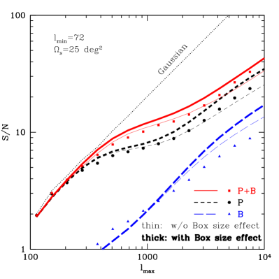
Refer to caption
Figure 15: The thick curves show the halo model predictions where we used the HSV effect taking into account of the effect of finite size of N-body simulations used in the ray-tracing simulations (see text for details). The thin curves and the simulation results are the same as in the left-hand panel of Fig. 10.