Photon splitting and Compton scattering in strongly magnetized hot plasma

Abstract

The process of photon splitting is investigated in the presence of strongly magnetized electron-positron plasma. The amplitude of the process is calculated in the general case of plasma with nonzero chemical potential and temperature. The polarization selection rules and corresponding partial amplitudes for allowed splitting channels are obtained in the case of charge-symmetric plasma. It is found that the new splitting channel forbidden in magnetized vacuum becomes allowed. The absorption rates of the photon splitting are calculated with taking into account the photon dispersion and wave function renormalization. In addition, the comparison of photon splitting and Compton scattering process is made. The influence of the reactions under consideration on the radiation transfer in the framework of the magnet ar model of a soft gamma repeater burst is discussed.

I Introduction

The process of photon splitting into two photons is a prominent example of the external active medium influence on the reactions with elementary particles. Though it is forbidden in vacuum by charged conjugation symmetry of quantum electrodynamics (QED), known as Furry’s theorem, it becomes allowed in the presence of an external electromagnetic field and/or plasma. In spite of the rather long history of the investigation  Adler:1970 ; Bialynicka:1970 ; Adler:1971 ; Ritus:1972 ; Stoneham:1979 ; Mentzel:1994 ; Adler:1996 ; Baier:1996 ; Chistyakov:1998 ; Weise:2004 (for a review see e.g. Papanian:1989 ; LaiHarding:2006 ) the process of photon splitting still attracts great interest concerning its possible applications.

It is remarkable, that such an exotic process may lead to observable physical manifestations in astrophysical objects. Its principal effect is to degrade photon energies and thereby soften gamma-ray spectra from neutron stars. In particular it is supposed that photon splitting could explain a peculiarity in the gamma-ray spectrum of some radio pulsars HBG:1997 .

Soft gamma repeaters (SGRs) and anomalous x-ray pulsars (AXPs) belong to the another class of astrophysical objects where the process of photon splitting could play an important role. There is a number of arguments that these objects are magnetars, a distinct class of neutron stars with magnetic field strength of $B\sim 10^{14}-10^{16}$ G Duncan:1992 , i.e. $B\gg B_{e}$, where $B_{e}=m^{2}/e\simeq 4.41\times 10^{13}$ G  is the critical magnetic field. It has been suggested that the degrading action of $\gamma\to\gamma\gamma$ could be responsible for the spectral cutoffs in the spectra of SGRs Baring:1995 ; Thompson:1995 .

There is one more interesting application of the process under consideration concerning the radio quiescence of SGRs and AXPs. Because photon splitting has no threshold, high-energy photons propagating at very small angles to the magnetic field in neutron star magnetospheres may split before reaching the threshold of pair production. Therefore, this process could change the production efficiency of electron-positron pairs required for a detectable radio emission BH:1998 ; Malofeev:2005 ; Istomin:2007 .

The process discussed here also plays an important role in the model of SGR burst Thompson:1995 ; Thompson:2001 . It is assumed the formation of the magnetically ”trapped fireball” in the near magnetosphere of a magnetar with hot $e^{+}e^{-}$-photon plasma occurs in local thermodynamic equilibrium.

Notice that in all of these astrophysical models the photon splitting process in the presence of strong magnetic field is considered in the environment which is non empty space. Instead the presence of considerably dense and hot electron-positron plasma is possible. This plasma could significantly change the photon splitting rate.

There are two ways in which a magnetized plasma influences the process under consideration. On the one hand, it modifies the photon dispersion properties. On the other hand it can change the process amplitude. The first effect has been studied previously in Refs. Adler:1971 ; Bulik:1998 . It was shown that in the case of the cold weakly magnetized plasma the process kinematics and polarization selection rules remain the same as in the magnetized vacuum if the electron density is not too large ($n_{e}\lesssim 10^{19}cm^{-3}$) Adler:1971 . In Bulik:1998 the probability of the photon splitting was calculated by including the plasma effects on the photon dispersion but using the process amplitude obtained in the weak magnetic field without plasma. It was found that the plasma influence in such an approach was negligibly small except the very narrow region of plasma and magnetic field parameter space.

The modification of the photon splitting amplitude in the presence of the magnetic field and plasma was considered in Elmfors:1998 ; Gies:2000 on the basis of the Euler-Heisenberg effective Lagrangian with taking account of thermal corrections in the one-loop and two-loop approximations correspondingly. It was noted that in the low-temperature limit the process $\gamma\to\gamma\gamma$ could compete with the other absorption reactions such as the Compton scattering process.

Another approach was applied in Martinez:2001 . Using the expansion of the electron propagator over of the magnetic field strength the amplitude and the absorption coefficient of photon splitting were calculated in the high-energy limit. The main conclusion of the paper was that the plasma effect was negligible. However, the estimations of the photon splitting absorption coefficients in the magnetic field presented in the paper in the high energy limit were incorrect because these expressions were applicable only in the low-energy approximations. Note that in Elmfors:1998 ; Gies:2000 ; Martinez:2001 the effects of the photon dispersion in magnetized plasma were not taken into account.

Unlike in the pure magnetic field, in the presence of plasma the photon can additionally scatter directly on electrons and positrons (Compton scattering). Moreover, in hot plasma the inverse process of photon merging, $\gamma\gamma\to\gamma$ also occurs. To be consistent, one has to compare all these processes under the same conditions. Previously, the Compton scattering in magnetic field without plasma was investigated in Herold:1979 ; Melrose:1983 ; Harding:1986 ; Harding:2000 . It was found that it became strongly anisotropic and essentially depended on a photon polarization. In Bulik:1997 , it was shown that the dispersion properties of a photon in strongly magnetized cold plasma could significantly influence the Compton scattering. The process of photon merging was considered in Thompson:1995 as one of the dominant number-photon changing process. The case of low energies and a strong magnetic field without plasma was investigated there.

Therefore, one can conclude that no self-consistent investigation of the photon splitting/merging and Compton scattering including modification of both dispersion relations and the process amplitude in magnetized plasma is currently available. Moreover, the case of the strong magnetic field, $B\gtrsim B_{e}$, which is relevant for the astrophysical applications has not been investigated for the process of photon splitting.

In the present paper we would like to fill in this gap. The processes of photon splitting/merging, $\gamma\leftrightarrow\gamma\gamma$ and Compton scattering are considered in the case of strongly magnetized $e^{+}e^{-}$-plasma, when the magnetic field strength $B$ is the maximal physical parameter, namely $\sqrt{eB}\gg T,\,\mu,\,\omega$. Here, $T$ is the plasma temperature, $\mu$ is the chemical potential, $\omega$ is the initial photon energy. Under these conditions, electrons and positrons in plasma occupy mainly the ground Landau level. The more accurate relation for the magnetic field and plasma parameters in this case can be obtained from the condition that the energy density of magnetic field must be much larger than plasma energy density Mikheev:2000 . For example, in ultrarelativistic plasma this condition leads to the following relation:

$$\frac{B^{2}}{8\pi}\gg\frac{\pi^{2}(n_{e^{-}}-n_{e^{+}})^{2}}{eB}+\frac{eBT^{2}}{12},$$

where $n_{e^{-}},n_{e^{+}}$ are the electron and positron number densities.

The paper is organized as follows. In Sec. II we calculate the photon splitting amplitude in the strong magnetic field and plasma in the general case of nonzero chemical potential and temperature. Taking in mind the possible application of our results to the magnetar model of SGR burst in all the following sections the case of the charge-symmetric electron-positron plasma ($\mu=0$) is considered. In Sec. III we perform an analysis of the $\gamma\to\gamma\gamma$ kinematics and consider the photon polarization selection rules. A numerical calculation of the photon splitting and merging absorption rates for different channels are presented in Sec. IV. In Sec. V we consider the process of Compton scattering and compare it with the photon splitting. Final comments and discussion of the obtained results and possible astrophysical applications are given in Sec. VI.

II Photon splitting amplitude

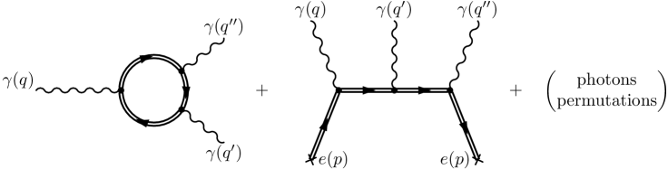
Figure 1: The Feynman diagrams for the photon splitting process in magnetized plasma. The cross at the end of the electron line symbolizes that the particle belongs to the medium.

The amplitude of the process under consideration can be presented as the sum of two terms,

$${\cal M}\,=\,{\cal M}_{B}+{\cal M}_{pl},$$ (1)

where ${\cal M}_{B}$ is the amplitude in the magnetized vacuum . The second term in (1) is the plasma contribution which can be treated as the photon coherent scattering from the real electrons and positrons with two photons emissions without change of their states (”forward“ scattering). These contributions are depicted by the Feynman diagrams in Fig. 1, where the internal double lines correspond to the electron propagator in a magnetic field. In the case of strongly magnetized plasma it is relevant to use the propagator in the asymptotic form Chistyakov:2002 :

$$S(x,y) = e^{i\Phi(x,y)}\hat{S}(x-y),$$ (2)

where

$$\hat{S}(X) = \hat{S}_{-}(X)+\hat{S}_{+}(X)+\hat{S}_{\mbox{\tiny$\bot$}}(X),$$ (3)

$$\hat{S}_{-}(X) \simeq \frac{ieB}{2\pi}\exp\left(-\frac{eBX_{\mbox{\tiny$\bot$}}^{2}}{4}\right)$$ (4)

$$\times \int\frac{d^{2}p}{(2\pi)^{2}}\,\frac{(p\gamma)_{\mbox{\tiny$\|$}}+m}{p_{\mbox{\tiny$\|$}}^{2}-m^{2}}\Pi_{-}e^{-i(pX)_{\mbox{\tiny$\|$}}},$$

$$\hat{S}_{+}(X) \simeq -\frac{i}{4\pi}\,[i(\gamma\,\partial/\partial X)_{\mbox{\tiny$\|$}}+m]\,\delta_{\mbox{\tiny$\|$}}^{2}(X)\,\Pi_{+}$$ (5)

$$\times \exp\left(\frac{eBX_{\mbox{\tiny$\bot$}}^{2}}{4}\right)\,\Gamma\left(0,\frac{eBX_{\mbox{\tiny$\bot$}}^{2}}{2}\right),$$

$$\hat{S}_{\mbox{\tiny$\bot$}}(X) \simeq -\frac{1}{2\pi}\,\delta_{\mbox{\tiny$\|$}}^{2}(X)\,\frac{(X\gamma)_{\mbox{\tiny$\bot$}}}{X_{\mbox{\tiny$\bot$}}^{2}}\exp\left(-\frac{eBX_{\mbox{\tiny$\bot$}}^{2}}{4}\right).$$ (6)

$$d^{2}p = dp_{0}dp_{3},\quad\Pi_{\pm}=\frac{1}{2}(1\pm i\gamma_{1}\gamma_{2}),$$

$$\Pi^{2}_{\pm} = \Pi_{\pm},\quad\quad\quad[\Pi_{\pm},(A\gamma)_{\mbox{\tiny$\|$}}]=0,$$

Here, $\gamma_{\alpha}$ are the Dirac matrices in the standard representation, $\Gamma(a,z)$ is the incomplete gamma function, $\Gamma(a,z)=\int\limits^{\infty}_{z}t^{a-1}e^{-t}dt,$ and

$$\Phi(x,y)=-e\int\limits_{x}^{y}d\xi_{\mu}\left[{\cal A}_{\mu}(\xi)+\frac{1}{2}F_{\mu\nu}(\xi-y)_{\mu}\right],$$ (7)

where ${\cal A}_{\mu}$ and $F_{\mu\nu}$ are the 4-potential and the tensor of the uniform magnetic field, correspondingly. Hereafter we use the notation: 4-vectors with the indices $\bot$ and $\parallel$ belong to the Euclidean (1, 2) subspace and the Minkowski (0, 3) subspace correspondingly, when the field $\bf B$ is directed along the third axis. Then for arbitrary 4-vectors $A_{\mu}$, $B_{\mu}$ one has

$$A_{\mbox{\tiny$\bot$}}^{\mu}=(0,A_{1},A_{2},0),\quad A_{\mbox{\tiny$\|$}}^{\mu}=(A_{0},0,0,A_{3}),$$

$$(AB)_{\mbox{\tiny$\bot$}}=(A\Lambda B)=A_{1}B_{1}+A_{2}B_{2},$$

$$(AB)_{\mbox{\tiny$\|$}}=(A\widetilde{\Lambda}B)=A_{0}B_{0}-A_{3}B_{3},$$

where the matrices $\Lambda_{\mu\nu}=(\varphi\varphi)_{\mu\nu}$,  $\widetilde{\Lambda}_{\mu\nu}=(\tilde{\varphi}\tilde{\varphi})_{\mu\nu}$ are constructed with the dimensionless tensor of the external magnetic field, $\varphi_{\mu\nu}=F_{\mu\nu}/B$, and the dual one, ${\tilde{\varphi}}_{\mu\nu}=\frac{1}{2}\varepsilon_{\mu\nu\rho\sigma}\varphi_{\rho\sigma}$. Matrices $\Lambda_{\mu\nu}$ and $\widetilde{\Lambda}_{\mu\nu}$ are connected by the relation $\widetilde{\Lambda}_{\mu\nu}-\Lambda_{\mu\nu}=g_{\mu\nu}=diag(1,-1,-1,-1)$, and play the role of the metric tensors in the perpendicular ($\bot$) and parallel ($\parallel$) subspaces respectively.

The double external lines in Fig. 1 correspond to the solution of the Dirac equation in a magnetic field for the electrons on the ground Landau level. For the choice of gauge ${\cal A}_{\mu}=(0,0,Bx,0),$ they are

$$\psi_{p\,\epsilon}=\frac{(eB)^{1/4}}{(\sqrt{\pi}2EL_{y}L_{z})^{1/2}}e^{-i\epsilon(Et-p_{y}y-p_{z}z)}e^{-\xi_{\epsilon}^{2}/2}u_{\epsilon}(p_{\mbox{\tiny$\|$}}),$$ (8)

where $\xi_{\epsilon}=\sqrt{eB}(x+\epsilon\frac{p_{y}}{eB})$, $\epsilon=\pm 1$ denotes the solutions for electron with positive and negative energy correspondingly, $E=\sqrt{p_{z}^{2}+m^{2}}$. The bispinor amplitudes are given by

$$u_{\epsilon}(p_{\mbox{\tiny$\|$}})=\frac{1}{\sqrt{E+\epsilon\,m}}\left(\begin{array}[]{c}(E+\epsilon\,m)\Psi\\ -p_{z}\Psi\end{array}\right),\,\Psi=\left(\begin{array}[]{c}0\\ 1\end{array}\right).$$ (13)

Then the plasma contribution can be obtained by the summation of the scattering diagrams in Fig. 1 over all electron and positron states with taking into account their distribution function in plasma. After rather lengthy but straightforward calculation we obtain the following expression for the amplitude:

$${\cal M}=\,\varepsilon_{\mu}(q)\varepsilon^{*}_{\nu}(q^{\prime\prime})\varepsilon^{*}_{\rho}(q^{\prime})\,\Pi_{\mu\nu\rho},$$ (14)

where

$$\Pi_{\mu\nu\rho} = eB\,\frac{e^{3}}{4\pi^{2}}\frac{(\tilde{\varphi}q)_{\mu}(\tilde{\varphi}q^{\prime\prime})_{\nu}(\tilde{\varphi}q^{\prime})_{\rho}}{(q^{\prime}\tilde{\varphi}q^{\prime\prime})}\Big{[}{\cal J}_{2}^{(-)}(q_{\mbox{\tiny$\|$}},q^{\prime}_{\mbox{\tiny$\|$}})\,-\,{\cal J}_{2}^{(-)}(-q^{\prime}_{\mbox{\tiny$\|$}},-q_{\mbox{\tiny$\|$}})\,-\,{\cal J}_{2}^{(-)}(-q^{\prime\prime}_{\mbox{\tiny$\|$}},q^{\prime}_{\mbox{\tiny$\|$}})\,-\,(q^{\prime}\leftrightarrow q^{\prime\prime})\Big{]}$$

$$- \frac{ie^{3}}{2\pi^{2}}\{(q^{\prime}\varphi q^{\prime\prime})\,[\pi_{\mu\nu\rho}+\upsilon_{\mu\nu\rho}]+(q^{\prime}{\cal G}(q^{\prime\prime}))_{\nu}\,\varphi_{\rho\mu}+\frac{1}{2}((q^{\prime\prime}-q^{\prime}){\cal G}(q))_{\mu}\,\varphi_{\nu\rho}+(q^{\prime\prime}{\cal G}(q^{\prime}))_{\rho}\,\varphi_{\nu\mu}$$

$$- {\cal G}_{\nu\rho}(q^{\prime\prime})\,(q^{\prime}\varphi)_{\mu}+{\cal G}_{\mu\nu}(q^{\prime\prime})\,(q\varphi)_{\rho}+{\cal G}_{\mu\rho}(q^{\prime})\,(q\varphi)_{\nu}-{\cal G}_{\nu\rho}(q^{\prime})\,(q^{\prime\prime}\varphi)_{\mu}-{\cal G}_{\mu\nu}(q)\,(q^{\prime\prime}\varphi)_{\rho}-{\cal G}_{\mu\rho}(q)\,(q^{\prime}\varphi)_{\nu}\$$

$$- \frac{i(\tilde{\varphi}q)_{\mu}(\tilde{\varphi}q^{\prime\prime})_{\nu}(\tilde{\varphi}q^{\prime})_{\rho}}{4(q^{\prime}\tilde{\varphi}q^{\prime\prime})}[q^{\prime 2}_{\mbox{\tiny$\bot$}}+q^{\prime\prime 2}_{\mbox{\tiny$\bot$}}+(q^{\prime}q^{\prime\prime})_{\mbox{\tiny$\bot$}}][{\cal J}_{2}^{(-)}(q_{\mbox{\tiny$\|$}},q^{\prime}_{\mbox{\tiny$\|$}})\,-\,{\cal J}_{2}^{(-)}(-q^{\prime}_{\mbox{\tiny$\|$}},-q_{\mbox{\tiny$\|$}})-{\cal J}_{2}^{(-)}(-q^{\prime\prime}_{\mbox{\tiny$\|$}},q^{\prime}_{\mbox{\tiny$\|$}})\,-\,(q^{\prime}\leftrightarrow q^{\prime\prime})]\}.$$

Here

$${\cal G}_{\mu\nu}(q) = \bigg{(}\tilde{\Lambda}_{\mu\nu}-\frac{q_{\mbox{\tiny$\|$}\mu}\,q_{\mbox{\tiny$\|$}\nu}}{q^{2}_{\mbox{\tiny$\|$}}}\bigg{)}\,{\cal G}(q_{\mbox{\tiny$\|$}}),$$ (16)

$${\cal G}(q_{\mbox{\tiny$\|$}}) = \left[H\!\!\left(\frac{q_{\mbox{\tiny$\|$}}^{2}}{4m^{2}}\right)+{\cal J}_{1}(q_{\mbox{\tiny$\|$}})\right],$$ (17)

$${\cal J}_{1}(q_{\mbox{\tiny$\|$}}) = 2q_{\mbox{\tiny$\|$}}^{2}m^{2}\int\frac{dp_{z}}{E}\,\frac{f_{-}(E)+f_{+}(E)}{q_{\mbox{\tiny$\|$}}^{4}-4(pq)_{\mbox{\tiny$\|$}}^{2}},$$ (18)

$${\cal J}_{2}^{(\pm)}(q_{\mbox{\tiny$\|$}},q^{\prime}_{\mbox{\tiny$\|$}}) = 2m^{2}\int\frac{dp_{z}}{E}\,\frac{f_{-}(E)\pm f_{+}(E)}{[q_{\mbox{\tiny$\|$}}^{2}+2(pq)_{\mbox{\tiny$\|$}}][q^{\prime 2}_{\mbox{\tiny$\|$}}+2(pq^{\prime})_{\mbox{\tiny$\|$}}]},$$

$f_{\mp}(E)\,=\,[e^{(E\,\mp\,\mu)/T}\,+\,1]^{-1}$ are the electron/positron distribution functions. The function $H(z)$ is defined as

$$H(z)=\frac{1}{\sqrt{z(1-z)}}\arctan{\sqrt{\frac{z}{1-z}}}-1,\,z\leq 1.$$ (20)

The expression for $\pi_{\mu\nu\rho}$ can be presented in the following form

$$\pi_{\mu\nu\rho} = \frac{1}{q^{2}_{\mbox{\tiny$\|$}}q^{\prime 2}_{\mbox{\tiny$\|$}}q^{\prime\prime 2}_{\mbox{\tiny$\|$}}}\Big{[}(q^{\prime}\tilde{\varphi}q^{\prime\prime})\big{\{}(\tilde{\varphi}q)_{\mu}(\tilde{\varphi}q^{\prime\prime})_{\nu}(\tilde{\varphi}q^{\prime})_{\rho}\pi_{\mbox{\tiny$\bot$}}+(\tilde{\varphi}q)_{\mu}(\widetilde{\Lambda}q^{\prime\prime})_{\nu}(\widetilde{\Lambda}q^{\prime})_{\rho}H-(\widetilde{\Lambda}q)_{\mu}(\tilde{\varphi}q^{\prime\prime})_{\nu}(\widetilde{\Lambda}q^{\prime})_{\rho}H^{\prime\prime}$$ (21)

$$- (\widetilde{\Lambda}q)_{\mu}(\widetilde{\Lambda}q^{\prime\prime})_{\nu}(\tilde{\varphi}q^{\prime})_{\rho}H^{\prime}\big{\}}+(q^{\prime}q^{\prime\prime})_{\mbox{\tiny$\|$}}(\widetilde{\Lambda}q)_{\mu}(\tilde{\varphi}q^{\prime\prime})_{\nu}(\tilde{\varphi}q^{\prime})_{\rho}(H^{\prime}-H^{\prime\prime})+(qq^{\prime\prime})_{\mbox{\tiny$\|$}}(\tilde{\varphi}q)_{\mu}(\tilde{\varphi}q^{\prime\prime})_{\nu}(\widetilde{\Lambda}q^{\prime})_{\rho}(H-H^{\prime\prime})$$

$$+ (qq^{\prime})_{\mbox{\tiny$\|$}}(\tilde{\varphi}q)_{\mu}(\widetilde{\Lambda}q^{\prime\prime})_{\nu}(\tilde{\varphi}q^{\prime})_{\rho}(H^{\prime}-H)\Big{]},$$

$$\pi_{\mbox{\tiny$\bot$}} = H^{\prime}+H^{\prime\prime}+H+2\{q^{2}_{\mbox{\tiny$\|$}}q^{\prime 2}_{\mbox{\tiny$\|$}}q^{\prime\prime 2}_{\mbox{\tiny$\|$}}-2m^{2}[q^{2}_{\mbox{\tiny$\|$}}(q^{\prime}q^{\prime\prime})_{\mbox{\tiny$\|$}}H-q^{\prime 2}_{\mbox{\tiny$\|$}}(qq^{\prime\prime})_{\mbox{\tiny$\|$}}H^{\prime}-q^{\prime\prime 2}_{\mbox{\tiny$\|$}}(qq^{\prime})_{\mbox{\tiny$\|$}}H^{\prime\prime}]\}$$ (22)

$$\times \{q^{2}_{\mbox{\tiny$\|$}}q^{\prime 2}_{\mbox{\tiny$\|$}}q^{\prime\prime 2}_{\mbox{\tiny$\|$}}-4m^{2}[q^{\prime 2}_{\mbox{\tiny$\|$}}q^{\prime\prime 2}_{\mbox{\tiny$\|$}}-(q^{\prime}q^{\prime\prime})^{2}_{\mbox{\tiny$\|$}}]\}^{-1}.$$

Here,

$$H\equiv H\!\!\left(\frac{q_{\mbox{\tiny$\|$}}^{2}}{4m^{2}}\right),\,H^{\prime}\equiv H\!\!\left(\frac{q^{\prime 2}_{\mbox{\tiny$\|$}}}{4m^{2}}\right),\,H^{\prime\prime}\equiv H\!\!\left(\frac{q^{\prime\prime 2}_{\mbox{\tiny$\|$}}}{4m^{2}}\right).$$

The expression for $\upsilon$ is

$$\upsilon_{\mu\nu\rho}=\pi_{\mu\nu\rho}\left[\pi_{\mbox{\tiny$\bot$}}\to\upsilon_{\mbox{\tiny$\bot$}},H\to{\cal J}_{1}(q_{\mbox{\tiny$\|$}}),H^{\prime}\to{\cal J}_{1}(q^{\prime}_{\mbox{\tiny$\|$}}),H^{\prime\prime}\to{\cal J}_{1}(q^{\prime\prime}_{\mbox{\tiny$\|$}})\right],$$

$$\upsilon_{\mbox{\tiny$\bot$}} = \frac{1}{(q^{\prime}\tilde{\varphi}q^{\prime\prime})^{2}}\Big{\{}(qq^{\prime})_{\mbox{\tiny$\|$}}(qq^{\prime\prime})_{\mbox{\tiny$\|$}}{\cal J}_{1}(q_{\mbox{\tiny$\|$}})-(qq^{\prime})_{\mbox{\tiny$\|$}}(q^{\prime}q^{\prime\prime})_{\mbox{\tiny$\|$}}{\cal J}_{1}(q^{\prime}_{\mbox{\tiny$\|$}})-(qq^{\prime\prime})_{\mbox{\tiny$\|$}}(q^{\prime}q^{\prime\prime})_{\mbox{\tiny$\|$}}{\cal J}_{1}(q^{\prime\prime}_{\mbox{\tiny$\|$}})$$ (23)

$$+ \frac{q^{2}_{\mbox{\tiny$\|$}}q^{\prime 2}_{\mbox{\tiny$\|$}}q^{\prime\prime 2}_{\mbox{\tiny$\|$}}}{4}\Big{[}{\cal J}_{2}^{(+)}(q_{\mbox{\tiny$\|$}},q^{\prime}_{\mbox{\tiny$\|$}})+{\cal J}_{2}^{(+)}(-q^{\prime}_{\mbox{\tiny$\|$}},-q_{\mbox{\tiny$\|$}})+{\cal J}_{2}^{(+)}(-q^{\prime\prime}_{\mbox{\tiny$\|$}},q^{\prime}_{\mbox{\tiny$\|$}})\,+\,(q^{\prime}\leftrightarrow q^{\prime\prime})\Big{]}\Big{\}}.$$

As it was noted in RCh05 , despite the fact that the amplitude (14) is obtained in the rest frame of plasma, it is possible to generalize it to the case when plasma moves as a whole along the magnetic field. It is well-known that this is implemented by introducing the velocity 4-vector $\upsilon_{\mu}$ ($\upsilon^{2}=1$) of the medium Fradkin:1965 ; Weldon:1982 in terms of which the amplitude can be written in a covariant form. In the presence of a magnetic field one should also introduce the condition for the absence of an electric field which can be written as $\upsilon_{\mu}\varphi_{\mu\nu}=0$ Shabad:1988 . We would like to emphasize that in contrast to the case of unmagnetized electron-positron plasma where introducing $u_{\mu}$ is required to present the two- and three-photon vertex in a covariant form Fradkin:1965 ; Weldon:1982 , in the presence of a magnetic field it is sufficient to take the substitutions $f_{\pm}(E)~{}\to~{}f_{\pm}(\upsilon p)$ in the electron and positron distribution functions in (18) and (LABEL:eq:J2). The fact is that an orthogonal basis can be constructed only from the field tensor and the 4-momentum vectorShabad:1988 :

$$b_{\mu}^{(1)}=\frac{(\varphi q)_{\mu}}{\sqrt{q^{2}_{\mbox{\tiny$\bot$}}}},\qquad b_{\mu}^{(2)}=\frac{(\tilde{\varphi}q)_{\mu}}{\sqrt{q^{2}_{\mbox{\tiny$\|$}}}},$$ (24)

$$b_{\mu}^{(3)}=\frac{q^{2}\,(\Lambda q)_{\mu}-q_{\mu}\,q^{2}_{\mbox{\tiny$\bot$}}}{\sqrt{q^{2}q^{2}_{\mbox{\tiny$\|$}}q^{2}_{\mbox{\tiny$\bot$}}}},\qquad b_{\mu}^{(4)}=\frac{q_{\mu}}{\sqrt{q^{2}}}.$$ (25)

With this basis any tensor can be represented in the covariant form.

The amplitude of the process written in the form (14) can be used to obtain the axion two-photons ($a\to\gamma\gamma$) and two-photons two-neutrino ($\gamma\gamma\to\nu\bar{\nu}$) interaction amplitude by making the substitutions

$${\cal M}_{a\to\gamma\gamma}={\cal M}\Big{(}\varepsilon_{\mu}\to q_{\mu}\frac{ig_{ae}}{2me},\Pi_{\mu\nu\rho}\to\tilde{\varphi}_{\mu\sigma}\Pi_{\sigma\nu\rho}\Big{)}$$ (26)

and

$${\cal M}_{\gamma\gamma\to\nu\nu} = {\cal M}\Big{(}\varepsilon_{\mu}\to j_{\mu}\frac{G_{F}}{\sqrt{2}e},\Pi_{\mu\nu\rho}\to C_{V}\Pi_{\mu\nu\rho}$$ (27)

$$+ C_{A}\tilde{\varphi}_{\mu\sigma}\Pi_{\sigma\nu\rho}\Big{)}$$

correspondingly RCh05 . Here, $C_{V}$ and $C_{A}$ are the vector and axial-vector constants of the effective $\nu\nu ee$ Lagrangian of the standard model,

$$C_{V}=\pm 1/2+2\sin^{2}\theta_{W},\quad C_{A}=\pm 1/2,$$

where $\theta_{W}$ is the Weinberg angle, the upper sign corresponds to an electron neutrino, the lower sign corresponds to muon and tau neutrinos, $j_{\mu}$ is the Fourier transform of the neutrino current, and $g_{ae}$ is the dimensionless axion-electron coupling constant.

III Kinematics and selection rules

As was mentioned in the Sec. I, the presence of magnetized plasma influences not only the process amplitude but the photon dispersion properties also and consequently it could change the kinematics of the process.

It is convenient to describe the propagation of the photon in any active medium in terms of the normal modes (eigenmodes). Then, the polarization and dispersion properties of the normal modes are connected with the eigenvectors and the eigenvalues of the polarization operator correspondingly.

To calculate the polarization operator, it is useful to represent it as an expansion over the basis (24), (25)

$${\cal P}_{\mu\nu}(q)=\sum\limits_{i,j=1}^{4}b^{(i)}_{\mu}b^{(j)}_{\nu}{\cal P}^{(i,j)}(q).$$ (28)

Note that the terms with $i,j=4$ may be omitted in (28) due to the gauge invariance of the polarization operator $q_{\mu}{\cal P}_{\mu\nu}(q)={\cal P}_{\mu\nu}(q)q_{\nu}=0$. In the magnetic field without plasma the polarization operator is known to be diagonal in such basis Shabad:1988 . Therefore one can write ${\cal P}^{(i,j)}(q)$ in the following way:

$${\cal P}^{(i,j)}(q)=\delta_{ij}{\cal P}_{B}^{(j)}(q)+{\cal P}_{pl}^{(i,j)}(q),$$ (29)

where ${\cal P}_{B}^{(j)}(q)$ is the magnetized vacuum contribution and ${\cal P}_{pl}^{(i,j)}(q)$ is the contribution arising from the photon forward scattering on electrons and positrons in plasma.

In the kinematic region where the absorption of the photon is disregarded, the polarization operator is the Hermitian matrix

$${\cal P}_{\mu\nu}(q)=[{\cal P}_{\nu\mu}(q)]^{*}.$$

This implies that the matrix ${\cal P}_{pl}^{(i,j)}(q)$ is also Hermitian

$${\cal P}_{pl}^{(i,j)}(q)=[{\cal P}_{pl}^{(j,i)}(q)]^{*}$$

in the same region.

Previously, the polarization operator in the presence of a magnetic field was investigated in several papers. In the strongly magnetized vacuum limit it could be taken e.g. from Shabad:1988 :

$${\cal P}_{B}^{(1)}(q) \simeq -\frac{\alpha}{3\pi}\,q_{\mbox{\tiny$\bot$}}^{2}-q^{2}\,\Lambda(B),$$ (30)

$${\cal P}_{B}^{(2)}(q) \simeq -\frac{2eB\alpha}{\pi}H\left(\frac{q^{2}_{\mbox{\tiny$\|$}}}{4m^{2}}\right)-q^{2}\,\Lambda(B),$$ (31)

$${\cal P}_{B}^{(3)}(q) \simeq -\,q^{2}\,\Lambda(B),$$ (32)

where

$$\Lambda(B)=\frac{\alpha}{3\pi}\,\left[1.792-\ln(B/B_{e})\right].$$

The polarization operator in magnetized plasma was studied in Rojas1979 ; Rojas1982 ; Shabad:1988 . However, to verify the method described in Sec. II we have calculated ${\cal P}_{pl}^{(i,j)}(q)$ in strongly magnetized plasma:

$${\cal P}_{pl}^{(1,1)}(q)=-\frac{2\alpha}{\pi eB}\int\frac{dp_{z}}{E}\,(pq)^{2}_{\mbox{\tiny$\|$}}\,[e^{E/T}\,+\,1]^{-1},$$ (33)

$${\cal P}_{pl}^{(2,2)}(q)=-\frac{8eB\alpha}{\pi}\,q_{\mbox{\tiny$\|$}}^{2}m^{2}\int\frac{dp_{z}}{E}\,\frac{[e^{E/T}\,+\,1]^{-1}}{q_{\mbox{\tiny$\|$}}^{4}-4(pq)_{\mbox{\tiny$\|$}}^{2}}\,,$$ (34)

$${\cal P}_{pl}^{(2,3)}(q)=-\frac{2\alpha}{\pi eB}\,\sqrt{\frac{q^{2}_{\mbox{\tiny$\bot$}}}{q^{2}}}\int\frac{dp_{z}}{E}\,(p\tilde{\varphi}q)\,(pq)_{\mbox{\tiny$\|$}}[e^{E/T}\,+\,1]^{-1},$$

$${\cal P}_{pl}^{(3,3)}(q)=\left(\frac{q^{2}_{\mbox{\tiny$\bot$}}}{q^{2}}-1\right)\,{\cal P}_{pl}^{(1,1)}(q),$$ (36)

$${\cal P}_{pl}^{(1,2)}(q) = {\cal P}_{pl}^{(1,3)}(q)=0.$$ (37)

To obtain the eigenvalues one should diagonalize the matrix ${\cal P}^{(i,j)}(q)$. It is seen from (33)-(37) that all of the nonzero components of the matrix ${\cal P}_{pl}^{(i,j)}(q)$ except ${\cal P}_{pl}^{(2,2)}(q)$ have an inverse dependence on the magnetic field strength. It means that these elements give a small contribution to diagonalized ${\cal P}^{(i)}(q)\equiv{\cal P}^{(i,i)}(q)$ in comparison with ${\cal P}_{B}^{(i)}(q)$. Finally the polarization operator eigenvalues can be written to within $O(B_{e}/B)$ in the following form:

$${\cal P}^{(1)}(q) \simeq {\cal P}_{B}^{(1)}(q),$$ (38)

$${\cal P}^{(2)}(q) \simeq {\cal P}_{B}^{(2)}(q)+{\cal P}_{pl}^{(2,2)}(q),$$ (39)

$${\cal P}^{(3)}(q) \simeq {\cal P}_{B}^{(3)}(q).$$ (40)

This result is in agreement with the previous one obtained by different methods in Refs. Rojas1979 ; Rojas1982 ; Shabad:1988 .

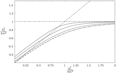
Figure 2: Photon dispersion laws in strong magnetic field $B/B_{e}=200$ and neutral plasma vs temperature: $T=1$ MeV (upper curve), $T=0.5$ MeV (middle curve), $T=0.25$ MeV (lower curve). Photon dispersion without plasma is depicted by the dashed line. The dotted line corresponds to the vacuum dispersion law, $q^{2}=0$. The angle $(\theta)$ between the photon momentum and the magnetic field direction is $\pi/2$.

The dispersion properties of the eigenmodes now can be found from the corresponding equations

$$q^{2}-{\cal P}^{(\lambda)}(q)=0\qquad(\lambda=1,2,3).$$ (41)

Their analysis shows that the waves with $\lambda=1,2$ and the polarization vectors

$$\varepsilon_{\mu}^{(1)}(q)=b_{\mu}^{(1)},\qquad\varepsilon_{\mu}^{(2)}(q)=b_{\mu}^{(2)}$$ (42)

are the only physical modes in the case under consideration, just as in a pure magnetic field. The third eigenmode, $\lambda=3$, does not correspond to any real wave Shabad:1988 . Indeed, the substitution of the expression for ${\cal P}^{(3)}(q)$ into (41) gives the equation that has the only solution $q^{2}=0$. Then the corresponding eigenvalue $b_{\mu}^{(3)}$ appears to be proportional to $q_{\mu}$ and, therefore, can be eliminated by a suitable gauge transformation.

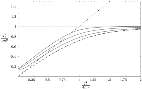
Figure 3: Photon dispersion laws in strong magnetic field $B/B_{e}=200$ and neutral plasma $(T=1\mbox{MeV})$ vs the angle between magnetic field direction and photon momentum: $\theta=\pi/2$ (upper curve), $\theta=\pi/6$ (middle curve), $\theta=\pi/12$ (lower curve). Photon dispersion without plasma is depicted by the dashed line. The dotted line corresponds to the vacuum dispersion law, $q^{2}=0$.

Let us consider the kinematics of the process under consideration. In the magnetized vacuum it is convenient to represent the dispersion law of the mode $\lambda$ in the form $q_{\mbox{\tiny$\|$}}^{2}=f^{(\lambda)}(q_{\mbox{\tiny$\bot$}}^{2})$ Shabad:1988 . From the energy conservation law it follows that a photon splitting is kinematically allowed only if the condition holds:

$$\sqrt{q_{\mbox{\tiny$\|$}}^{2}}\geq\sqrt{q^{\prime 2}_{\mbox{\tiny$\|$}}}+\sqrt{q^{\prime\prime 2}_{\mbox{\tiny$\|$}}}\,.$$ (43)

Using the dispersion law it can be written as

$$\sqrt{f^{(\lambda)}(q_{\mbox{\tiny$\bot$}}^{2}})\geq\sqrt{f^{(\lambda^{\prime})}(q^{\prime 2}_{\mbox{\tiny$\bot$}})}+\sqrt{f^{(\lambda^{\prime\prime})}(q^{\prime\prime 2}_{\mbox{\tiny$\bot$}})}.$$ (44)

The analysis of the dispersion equation solutions shows that in the region below the pair creation threshold ($q^{2}_{\mbox{\tiny$\|$}}~{}=~{}4m^{2}$) the functions $f^{(\lambda)}(q_{\mbox{\tiny$\bot$}}^{2})$ are the monotonic single-valued and the inequalities

$$f^{(\lambda)}(q_{\mbox{\tiny$\bot$}}^{2})\leq q_{\mbox{\tiny$\bot$}}^{2},\quad f^{(2)}(q_{\mbox{\tiny$\bot$}}^{2})<f^{(1)}(q_{\mbox{\tiny$\bot$}}^{2})$$ (45)

hold throughout the interval $0\leq q_{\mbox{\tiny$\bot$}}^{2}\leq\infty$. From these conditions and the inequality (43), it immediately follows that only the splitting channels $\gamma_{1}\to\gamma_{2}\gamma_{2},\gamma_{1}\to\gamma_{1}\gamma_{2}$ are kinematically allowed below the pair creation threshold Adler:1971 ; Shabad:1983 ; Usov:2002 ; Chistyakov:1998 . It coincide with Adler’s selection rules in a weak magnetic field Adler:1971 .

It is usually assumed that the photon splitting can be neglected in the region $q^{2}_{\mbox{\tiny$\|$}}>4m^{2}$ in comparison with the process of the pair creation $\gamma\to e^{+}e^{-}$. This is true in the case of a not too strong magnetic field, $B\lesssim B_{e}$, when the resonances of the polarization operator corresponding to the creation thresholds of electrons and positrons on the different Landau levels are close to each other. In a strong magnetic field, the gap between the two first resonances becomes wide. In this case the 2-mode photon can decay into the $e^{+}e^{-}$-pair just above the first resonance $q^{2}_{\mbox{\tiny$\|$}}=4m^{2}$, whereas the lowest 1-mode pair creation threshold is $q^{2}_{\mbox{\tiny$\|$}}=4m^{2}(1/2+\sqrt{1/2+B/B_{e}})^{2}\simeq 4m^{2}B/B_{e}$. Therefore in the kinematical region $4m^{2}<q^{2}_{\mbox{\tiny$\|$}}<4m^{2}B/B_{e}$ the only QED absorption mechanism for the 1-mode is the photon splitting. It is not difficult to understand that the 1-mode photon in this region can split by the same channels $\gamma_{1}\to\gamma_{2}\gamma_{2},\gamma_{1}\to\gamma_{1}\gamma_{2}$ if the 2-mode photons in the final state are created with $q^{2}_{\mbox{\tiny$\|$}}$ below $4m^{2}$ Chistyakov:1998 . Strictly speaking, the 2-mode photon also can split above the pair creation threshold. However, as it was mentioned above, the corresponding absorption rates are negligible in comparison with the rate of the process $\gamma_{2}\to e^{+}e^{-}$.

The presence of plasma could change the selection rules described above. A comparison of the Eqs. (30)-(32) and (38)-(40) shows that only the eigenvalue ${\cal P}^{(2)}(q)$ is modified in plasma. It means that the dispersion law of the mode 1 photon is the same as in the magnetized vacuum, where it is spacelike and its deviation from the vacuum law, $q^{2}=0$, is negligibly small. On the other hand, the dispersion properties of the mode 2 photon essentially differs from the ones in magnetized vacuum. In this case the dispersion law in the form of the relation between $q^{2}_{\mbox{\tiny$\|$}}$ and $q^{2}_{\mbox{\tiny$\bot$}}$ additionally depends on the angle between the magnetic field direction and the photon momentum $q^{2}_{\mbox{\tiny$\|$}}=f^{(2)}(q^{2}_{\mbox{\tiny$\bot$}},\theta)$.

In Figs. 2 and 3, the photon dispersion laws are depicted both in a strong magnetic field and in magnetized plasma at various temperatures, angles and photon momenta. One can see that contrary to the pure magnetic field case in plasma there is the region with $q^{2}>0$ below the pair creation threshold where the inequalities hold, opposite of the relations (45). It is connected with the appearance of the plasma frequency in the presence of real electrons and positrons which can be defined from the equation

$$\omega_{pl}^{2}-{\cal P}^{(2)}(\omega_{pl},{\mathbf{k}}\to 0)=0.$$ (46)

These facts lead to new polarization selection rules: in the region $q^{2}>0$, a new photon splitting channel $\gamma_{2}\to\gamma_{1}\gamma_{1}$ forbidden in the magnetic field without plasma is possible, while the splitting channels $\gamma_{1}\to\gamma_{2}\gamma_{2}$ and $\gamma_{1}\to\gamma_{1}\gamma_{2}$ allowed in the pure magnetic field, are forbidden. In the region $q^{2}<0$ polarization selection rules are the same ones as in a magnetized vacuum. Strictly speaking, the dependence of the dispersion law on the angle between magnetic field direction and photon momentum could lead to the permission of the additional splitting channel, e.g. $\gamma_{2}\to\gamma_{2}\gamma_{2}$ or $\gamma_{2}\to\gamma_{1}\gamma_{2}$. However the numerical analysis shows that these transitions are forbidden under considered conditions.

As it follows from (39), the eigenvalue of the polarization operator ${\cal P}^{(2)}(q)$ has singular behavior in the vicinity of the pair-creation threshold:

$${\cal P}^{(2)}(q)\simeq-\frac{2\alpha\,eB\,m}{\sqrt{4m^{2}-q_{\mbox{\tiny$\|$}}^{2}}}\,\tanh\frac{\omega}{4T}.$$ (47)

This fact leads to the necessity of taking into account of a wave function renormalization for the photon of mode 2

$$\varepsilon_{\alpha}^{(2)}(q)\to\varepsilon_{\alpha}^{(2)}(q)\sqrt{Z_{2}},\quad Z^{-1}_{2}=1-\frac{\partial{\cal P}^{(2)}(q)}{\partial\omega^{2}}.$$ (48)

The partial amplitudes for the channels $\gamma_{1}\to\gamma_{1}\gamma_{2}$, $\gamma_{1}\to\gamma_{2}\gamma_{2}$ and $\gamma_{2}\to\gamma_{1}\gamma_{1}$ could be obtained from (14) by substitution of the corresponding polarization vectors (42)

$${\cal M}_{\lambda\to\lambda^{\prime}\lambda^{\prime\prime}}=\,\varepsilon^{(\lambda)}_{\mu}(q)\varepsilon^{(\lambda^{\prime})*}_{\rho}(q^{\prime})\varepsilon^{(\lambda^{\prime\prime})*}_{\nu}(q^{\prime\prime})\,\Pi_{\mu\nu\rho}.$$ (49)

Then,

$${\cal M}_{1\to 12} = -i4\pi\left(\frac{\alpha}{\pi}\right)^{\mbox{\tiny$3/2$}}\frac{(q^{\prime}\varphi q^{\prime\prime})(q^{\prime}\tilde{\varphi}q^{\prime\prime})}{[q^{\prime 2}_{\mbox{\tiny$\bot$}}q^{\prime\prime 2}_{\mbox{\tiny$\|$}}q^{2}_{\mbox{\tiny$\bot$}}]^{\mbox{\tiny$1/2$}}}{\cal G}(q^{\prime\prime}_{\mbox{\tiny$\|$}}),$$ (50)

$${\cal M}_{1\to 22} = -i4\pi\left(\frac{\alpha}{\pi}\right)^{\mbox{\tiny$3/2$}}\frac{(q^{\prime}q^{\prime\prime})_{\mbox{\tiny$\|$}}}{[q^{\prime 2}_{\mbox{\tiny$\|$}}q^{\prime\prime 2}_{\mbox{\tiny$\|$}}q^{2}_{\mbox{\tiny$\bot$}}]^{\mbox{\tiny$1/2$}}}$$

$$\times \left\{(qq^{\prime\prime})_{\mbox{\tiny$\bot$}}{\cal G}(q^{\prime}_{\mbox{\tiny$\|$}})+(qq^{\prime})_{\mbox{\tiny$\bot$}}{\cal G}(q^{\prime\prime}_{\mbox{\tiny$\|$}})\right\},$$

$${\cal M}_{2\to 11} = {\cal M}_{1\to 12}(q\leftrightarrow q^{\prime\prime}),\quad$$ (52)

where ${\cal G}(q_{\mbox{\tiny$\|$}})$ is given by Eq. (17).

IV Photon absorption rate

To analyze the efficiency of the process under consideration and to compare it with other competitive reactions we calculate the photon absorption rate due to photon splitting which can be defined in the following way:

$$W_{\lambda\to\lambda^{{}^{\prime}}\lambda^{{}^{\prime\prime}}}=\frac{g_{\lambda^{\prime}\lambda^{\prime\prime}}}{32\pi^{2}\omega_{\lambda}}\int\left|{\cal M}_{\lambda\to\lambda^{{}^{\prime}}\lambda^{{}^{\prime\prime}}}\right|^{2}Z_{\lambda}Z_{\lambda^{{}^{\prime}}}Z_{\lambda^{{}^{\prime\prime}}}$$

$$\times(1+f_{\omega^{\prime}})(1+f_{\omega^{\prime\prime}})$$

$$\times\delta(\omega_{\lambda}({\bf k})-\omega_{\lambda^{{}^{\prime}}}({\bf k}-{\bf k^{{}^{\prime\prime}}})-\omega_{\lambda^{{}^{\prime\prime}}}({\bf k^{{}^{\prime\prime}}}))\frac{d^{3}k^{{}^{\prime\prime}}}{\omega_{\lambda^{{}^{\prime}}}\omega_{\lambda^{{}^{\prime\prime}}}},$$ (53)

where $f_{\omega}=[e^{\omega/T}-1]^{-1}$ is the photons distribution function and the factor $g_{\lambda^{\prime}\lambda^{\prime\prime}}=1-(1/2)\,\delta_{\lambda^{\prime}\lambda^{\prime\prime}}$ is inserted to account for the possible identity of the final photons.

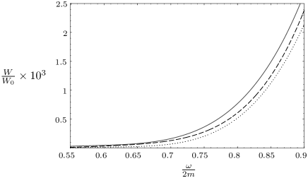
Figure 4: Absorption rate of the channel $\gamma_{1}\to\gamma_{1}\gamma_{2}$ in strong magnetic field ($B/B_{e}=100$) at temperatures 50 keV (solid line) and 250 keV (dotted line). The dashed curve represents the probability in a pure magnetic field ($T=\mu=0$) Chistyakov:1998 . $W_{0}\,=\,(\alpha/\pi)^{3}\,m\simeq 3.25\cdot 10^{2}cm^{-1}$and $\theta=\pi/2$.

IV.1 Channels $\gamma_{1}\to\gamma_{1}\gamma_{2}$ and $\gamma_{1}\to\gamma_{2}\gamma_{2}$

In general case the reaction rates (53) can be calculated only numerically. However in some limiting cases it is possible to obtain the simple expression for the rates. Analysis shows that in the low-temperature ($T\ll m$) and low-energy ($\omega\ll m$) limits the modification of the amplitudes (50)-(52) in the presence of plasma is small in comparison with the expressions in pure magnetic field. The main manifestation of plasma influence arises from taking account of 2-mode photon dispersion in energy conservation law. In the limit under consideration it is convenient to use the following approximation for photon dispersion law:

$$q^{2}_{\mbox{\tiny$\|$}}\simeq\omega^{2}_{pl}\sin^{2}{\theta}+(1-\xi)q^{2}_{\mbox{\tiny$\bot$}},$$ (54)

where

$$\omega^{2}_{pl} = \frac{4\alpha\pi}{m}n_{e},$$ (55)

$$n_{e} \simeq eB\sqrt{\frac{mT}{2\pi^{3}}}\,e^{-m/T}.$$ (56)

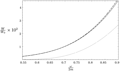
Figure 5: Absorption rate of the channel $\gamma_{1}\to\gamma_{2}\gamma_{2}$ for the same parameters and notation as those in Fig.4.

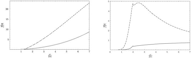
Figure 6: The dependence of the absorption rates of channel $\gamma_{1}\to\gamma_{1}\gamma_{2}$ (left panel) and $\gamma_{1}\to\gamma_{2}\gamma_{2}$ (right panel) on energy in a strong magnetic field $B/B_{e}\,=\,200$ and neutral $(T\,=\,1\mbox{MeV})$ plasma. The dashed line corresponds to the probability in the pure magnetic field $(T\,=\,0)$ Chistyakov:1998 . The asymptote (IV.1) is depicted by dots. Here, $\theta=\pi/2$.

Here $n_{e}$ is the number of electron and positron density in strongly magnetized, charge-symmetric low-temperature plasma; $\theta$ is the angle between the photon momentum ${\bf k}$ and the magnetic field direction ${\bf B}$; $\xi=\frac{\alpha}{3\pi}\frac{B}{B_{e}}$ is the parameter characterizing magnetic field influence (it is assumed small in the limit under consideration).

Then, using the photon dispersion law (54) one can obtain the following expressions of photon splitting rates in a low-temperature case:

$$W_{1\to 12} \simeq \frac{\alpha^{3}\xi^{2}m}{288\pi^{2}}\,\left(\frac{T}{m}\right)^{5}\,{\cal F}_{1}\left(\frac{\omega}{T},\sqrt{1-u^{2}}\right),$$ (57)

$$W_{1\to 22} \simeq \frac{\alpha^{3}m}{72\pi^{2}}\,\left(\frac{T}{m}\right)^{5}\,{\cal F}_{2}\left(\frac{\omega}{T},\sqrt{1-u^{2}}\right),$$ (58)

where $u\,=\,\cos{\theta}$ and ${\cal F}_{1}(y,z)$ and ${\cal F}_{2}(y,z)$ are the integrals

$${\cal F}_{1}(y,z) = \frac{1}{y^{2}z}\,\int\limits_{\delta}^{yz}\frac{dx}{x^{2}}\,\frac{[x^{2}-\delta^{2}]^{4}}{[1-\exp(-x)]}$$ (59)

$$\times \frac{1}{[1-\exp(x-y)(1-\frac{\xi}{2y}(x^{2}-\delta^{2}))]},$$

$${\cal F}_{2}(y,z) = z\,\Theta(yz-2\delta)\int\limits_{\delta}^{\lambda(y,z)}dx\frac{[x(yz-x)-\delta^{2}]^{2}}{[1-\exp(-x)]}$$ (60)

$$\times \frac{1}{[1-\exp(x-y)(1-\frac{\xi}{2y}(x^{2}-\delta^{2}))]},$$

where

$$\lambda(y,z)=\frac{yz}{2}+\sqrt{\frac{y^{2}z^{2}}{4}-\delta^{2}}$$

and $\delta\equiv(\omega_{pl}/T)\xi^{-1/2}$; $\Theta(x)$ is theta function. Note, that in the limit $T\to 0$ one can obtain the expressions of photon splitting rates in strongly magnetized vacuum:

$$W_{1\to 12} \simeq \frac{\alpha^{3}\xi^{2}m}{2016\pi^{2}}\left(\frac{\omega}{m}\right)^{5}\sin^{6}\theta,$$ (61)

$$W_{1\to 22} \simeq \frac{\alpha^{3}m}{2160\pi^{2}}\left(\frac{\omega}{m}\right)^{5}\sin^{6}\theta,$$ (62)

The expression (58) may be easily derived from Eq. (23) of Adler:1971 (see also, e.g., Thompson:1995 , HBG:1997 ). To our knowledge the expression of the photon splitting rate for channel $\gamma_{1}\to\gamma_{1}\gamma_{2}$ in low-energy limit was not published before.

The comparison of photon splitting rates in strongly magnetized plasma (57), (58) and vacuum (61), (62) shows that electron-positron background and thermal photons have an opposite influence on the process under consideration. On one hand, the presence of $e^{+}e^{-}$ plasma leads to the decreasing of the amplitude and phase space of the reactions. On the other hand photon splitting rates increase due to bosonic final state stimulation effect. From the analysis of the result obtained (57), (58) follows that in the low-energy and low-temperature limit the plasma influence leads to the increase of the photon splitting rate beside the magnetized vacuum case. However, numerical calculations show that in the range $\omega\sin{\theta}\leq 2m$ rates decrease with a temperature increase and become smaller than those in pure magnetic field at some values of temperature (see the dotted line in Figs. 4 and 5).

Figure 7: The dependence of the absorption rates of the channels $\gamma_{1}\to\gamma_{1}\gamma_{2}$ (left panel) and $\gamma_{1}\to\gamma_{2}\gamma_{2}$ (right panel) on an angle between initial photon momentum and magnetic field direction at different initial photon energies ($B/B_{e}\,=\,200,T\,=\,1\mbox{MeV}$). The numbers above the curves correspond to the values of the ratio $\omega/2m$.

The results obtained show that the rate $W_{1\to 12}$ is considerably suppressed compared to $W_{1\to 22}$. The reason for this is the same as in the pure magnetic field case. In the energy region $\omega\sin{\theta}\leq 2m$ the kinematics of the processes under consideration is closed to the collinear one. In this case, it is easy to show that in contrast to the channel $\gamma_{1}\to\gamma_{2}\gamma_{2}$ the amplitude ${\cal M}_{112}$ (50) contains terms $(q^{\prime}\varphi q^{\prime\prime})\sim(q^{\prime}\tilde{\varphi}q^{\prime\prime})\sim\Delta\phi$, where $\Delta\phi$ is the angular separation between the two photons in the final state. At low-photon energies $\Delta\phi\sim\sqrt{\xi}\sin{\theta}$ and $W_{1\to 12}$ is suppressed by the factor $\xi^{2}\sin^{2}{\theta}\ll 1$ in comparison with $W_{1\to 22}$.

The situation changes dramatically when the energy of the initial photons becomes larger than $2m/\sin{\theta}$. Let us consider the limit $m^{2}\ll\omega^{2}\,\sin^{2}{\theta}\leq eB$. The analysis shows that in this case the main contribution to the probability of the processes comes from the kinematical region in close vicinity to the pair creation threshold of the 2-mode photon because the amplitudes (50) and (III) have the square root singular behavior in this region. As a consequence, the corresponding splitting rates might contain the pole singularity. However, taking account of the photon wave function renormalization corrects the situation. Indeed, in the limit $q^{2}_{\mbox{\tiny$\|$}}\to 4m^{2}$ it can be shown that the production of the singular function ${\cal G}(q_{\mbox{\tiny$\|$}})$ in the amplitudes (50), (III) and the square root of the renormalization function $Z_{2}$ is the regular function:

$${\cal G}(q_{\mbox{\tiny$\|$}})\sqrt{Z_{2}}\simeq\frac{\sqrt{2}\pi m}{\sqrt{q^{2}_{\mbox{\tiny$\bot$}}}}\,\tanh{\frac{\omega}{4T}}.$$

Note that in this region the 2-mode photon dispersion law is simplified and can be defined by the following relationship:

$$\sqrt{1-\frac{q^{2}_{\mbox{\tiny$\|$}}}{4m^{2}}}\simeq\alpha\,\frac{eB}{q^{2}_{\mbox{\tiny$\bot$}}}\,\tanh{\frac{\omega}{4T}}$$ (63)

Taking in mind these facts, we obtain the following approximation of the photon splitting rates:

$$W_{1\to 12} \simeq \frac{\alpha^{3}T^{2}}{4\omega(1-u^{2})}$$

$$\times \left[(1\,-\,u)^{2}\,{\cal F}_{3}\left(\frac{\omega(1+u)}{2T}\right)\,+\,(u\to-u)\right],$$

$$W_{1\to 22} \simeq \frac{\alpha^{3}m^{2}}{4\omega}\,\frac{1}{1\,-\,\exp{\left[-\frac{\omega}{T}(1\,-\,u)\right]}}$$

$$\times \frac{1}{1\,-\,\exp{\left[-\frac{\omega}{T}(1\,+\,u)\right]}}$$

$$\times \left\{\tanh^{2}\left[\frac{\omega}{8T}(1\,-\,u)\right]\,+\,(u\to-u)\right\},$$

where

$${\cal F}_{3}(z)\,=\,\int\limits_{0}^{z}\frac{x\tanh^{2}(x/4)\,dx}{[1\,-\,\exp{(-x)}]\,[1\,-\,\exp{(x\,-\,\omega/T)}]},$$ (66)

Again, in the limit $T\to 0$ these formulas turn into the expressions of the photon splitting probabilities in strong magnetic field in the absence of plasma Chistyakov:1998 :

$$W_{1\to 12} \simeq \frac{\alpha^{3}\omega\sin^{2}{\theta}}{16},$$ (67)

$$W_{1\to 22} \simeq \frac{\alpha^{3}m^{2}}{2\omega},$$ (68)

from which follow that at high-photon energies the rate of the channel $\gamma_{1}\to\gamma_{1}\gamma_{2}$ dominates over $W_{1\to 22}$. The analysis of the approximations (IV.1), (IV.1) and numerical calculations (see Fig. 6) show that the same relation between channel rates is kept also in the presence of plasma. One can see also that photon splitting rates in plasma is suppressed in comparison with pure magnetic field results at high energies of the splitting photon.

In addition to the energy dependence of photon splitting probability it is interesting also to consider the dependence on angle between initial photon momentum and magnetic field direction. It is important, e.g., in the problem of radiation transfer in strongly magnetized plasma (see Sec. VI). The results of the numerical calculation are depicted in Fig. 7 for different energies of the initial photon. It is interesting to note that rate of the channel $\gamma_{1}\to\gamma_{1}\gamma_{2}$ attains its maximum at $\theta=\pi/2$ while $W_{1\to 22}$ may have global maximum at $\theta<\pi/2$.

IV.2 Channel $\gamma_{2}\to\gamma_{1}\gamma_{1}$

Figure 8: Absorption rate of the channel $\gamma_{2}\to\gamma_{1}\gamma_{1}$ in a strong magnetic field ($B/B_{e}=200$) at temperatures of 1 MeV (solid line) and 500 keV (dashed line). Here, $\theta=\pi/2$.

As it was found in Sec. III in the presence of strongly magnetized plasma the ”new” photon splitting channel $\gamma_{2}\to\gamma_{1}\gamma_{1}$ forbidden in the pure magnetic field, becomes open. According to (52) and (53) the absorption rate of the channel $\gamma_{2}\to\gamma_{1}\gamma_{1}$ can be presented as

$$W_{2\to 11}=\frac{\alpha^{3}}{8\pi^{2}}\,Z_{2}\,{\cal G}^{2}(q_{\mbox{\tiny$\|$}})\,\frac{q_{\mbox{\tiny$\bot$}}^{2}}{\omega}\,{\cal F}_{4}\left(\sqrt{\frac{q_{\mbox{\tiny$\|$}}^{2}}{q_{\mbox{\tiny$\bot$}}^{2}}}\right)\,\Theta(q^{2})\,,$$ (69)

where

$${\cal F}_{4}(z) = \frac{4z^{3}}{\pi}\,\int^{1+z}_{1-z}dx\int^{y_{0}}_{0}dy\frac{y^{2}\sqrt{y_{0}^{2}-y^{2}}}{(x^{2}+z^{2}y^{2})[(2-x)^{2}+z^{2}y^{2}]}\big{\{}(1+f_{\omega_{+}})(1+f_{\omega-\omega_{+}})+(\omega_{+}\to\omega_{-})\big{\}}\,,$$

$$\omega_{\pm} = \frac{1}{2z^{2}}\,\bigg{[}\omega(z^{2}-1+x)\pm q_{z}z^{2}\,\sqrt{y_{0}^{2}-y^{2}}\,\bigg{]}\,,y_{0}=\frac{\sqrt{z^{2}-1}}{z^{2}}\,\sqrt{z^{2}-(1-x)^{2}}\,,\quad z=\sqrt{\frac{q_{\mbox{\tiny$\|$}}^{2}}{q_{\mbox{\tiny$\bot$}}^{2}}}\,.$$

If one can neglect the effect of final photons stimulation emission $(f_{\omega^{\prime}}\,=\,f_{\omega^{\prime\prime}}\,=\,0)$ the expression for the function ${\cal F}_{4}(z)$ is considerably simplified:

$${\cal F}_{4}(z)\,=\,2\ln{z}\,-\,1\,+\,z^{-2}\,.$$

In Fig. 8 the absorption rate of the channel $\gamma_{2}\to\gamma_{1}\gamma_{1}$ as a function of the initial photon energy is depicted for the case of the photon propagation across magnetic field direction at temperatures of 1 MeV and 500 keV. One can see that in contrast to the $\gamma_{1}\to\gamma_{1}\gamma_{2}$ and $\gamma_{1}\to\gamma_{2}\gamma_{2}$ channels behavior $\gamma_{2}\to\gamma_{1}\gamma_{1}$ the splitting rate decreases rapidly with decreasing temperature. This is due to an increase of the kinematically allowed region ($q^{2}>0$) for the channel under consideration leading to the growth of the process phase space volume with temperature increasing.

The dependence of the $\gamma_{2}\to\gamma_{1}\gamma_{1}$ splitting rate on an angle between initial photon momentum and magnetic field direction at temperature 1 MeV is depicted in Fig. 9. Note that in the range $\pi/4\lesssim\theta\leq\pi/2$, $W_{2\to 11}$ weakly depends on the angle.

IV.3 Photon merging

Due to the finite photon density in electron-positron plasma the inverse process of photon merging $\gamma\gamma\to\gamma$ should be taking into account, e.g., in radiation transfer problem Thompson:1995 . One can define the absorption rate of the process under consideration in the same manner as for the photon splitting:

$$W_{\lambda\lambda^{{}^{\prime}}\to\lambda^{{}^{\prime\prime}}}=\frac{1}{32\pi^{2}\omega_{\lambda}}\int\left|{\cal M}_{\lambda\lambda^{{}^{\prime}}\to\lambda^{{}^{\prime\prime}}}\right|^{2}Z_{\lambda}Z_{\lambda^{{}^{\prime}}}Z_{\lambda^{{}^{\prime\prime}}}$$

$$\times f_{\omega^{\prime}}(1+f_{\omega^{\prime\prime}})$$

$$\times\delta(\omega_{\lambda}({\bf k})+\omega_{\lambda^{{}^{\prime}}}({\bf k}+{\bf k^{{}^{\prime\prime}}})-\omega_{\lambda^{{}^{\prime\prime}}}({\bf k^{{}^{\prime\prime}}}))\frac{d^{3}k^{{}^{\prime\prime}}}{\omega_{\lambda^{{}^{\prime}}}\omega_{\lambda^{{}^{\prime\prime}}}},$$ (70)

where amplitudes ${\cal M}_{\lambda\lambda^{{}^{\prime}}\to\lambda^{{}^{\prime\prime}}}$ can be obtained from (50)-(52) using crossing symmetry. We have made numerical analysis of the photon merging rate for kinematically allowed channels in the case of the initial photon propagation across magnetic field direction. The results are presented on Figs. 10 and 11. As can be seen from these figures, the contribution of the channel $\gamma_{1}\gamma_{2}\to\gamma_{1}$ to the absorption rate is negligible at low temperature, however it dominates in more hot plasma (see Fig. 11). On the other hand, the channel $\gamma_{2}\gamma_{2}\to\gamma_{1}$ leading at the temperature $T=50$ keV is kinematically suppressed at higher temperatures. The photon splitting channels are also suppressed in hot plasma in the region $\omega\lesssim 2m$. It is interesting to note that $W_{21\to 1}$ has resonant amplification in the vicinity of the pair creation threshold, $\omega\simeq 2m$.

We can see now that in the presence of hot plasma the process of photon merging could be an effective particle attenuation mechanism, whereas at relatively low temperatures ($T\simeq 50$ keV) both photon splitting and photon merging processes play the main role in the change of photon numbers.

V Compton scattering

Figure 9: The dependence of the absorption rate of the channel $\gamma_{2}\to\gamma_{1}\gamma_{1}$ on an angle between initial photon momentum and magnetic field direction at different initial photon energies ($B/B_{e}\,=\,200,T\,=\,1\mbox{MeV}$). The numbers above the curves correspond to the values of the ratio $\omega/2m$.

Compton scattering is the other type of photon reaction competing with photon splitting (merging). The process of photon scattering in a strongly magnetized plasma, when the initial photon propagates across magnetic field, at the different temperatures and taking into account the photon dispersion and wave function renormalization was investigated recently (see RCh09 and references therein). Here, we generalize our results to the case of arbitrary angle between initial photon momenta and magnetic field direction.

To calculate the amplitude of the process in a strong magnetic field one should use the Dirac equation solutions at the ground Landau level (8). However, for virtual electron it is necessary to use the exact propagator, e.g., in the form of the Landau level decomposition Chodos:1990 ; KuznOkrug:2011 . As a result we obtain

$${\cal M}_{\lambda\to\lambda^{\prime}}=-4\pi\alpha\exp\left[-\frac{q_{\mbox{\tiny$\bot$}}^{2}+q_{\mbox{\tiny$\bot$}}^{\prime 2}+2i(q\varphi q^{\prime})}{4eB}\right]$$ (71)

$$\times\sum_{n=0}^{\infty}\,\frac{\varepsilon^{*(\lambda^{\prime})}_{\alpha}(q^{\prime})\varepsilon^{(\lambda)}_{\beta}(q)\,T_{\alpha\beta}^{n}}{q_{\mbox{\tiny$\|$}}^{2}+2(pq)_{\mbox{\tiny$\|$}}-2eBn}+(q\leftrightarrow-q^{\prime}),$$

where

$$T_{\alpha\beta}^{n}=\frac{2m}{\sqrt{-Q_{\mbox{\tiny$\|$}}^{2}}}\big{\{}S_{n}[-(q\tilde{\Lambda})_{\alpha}(Q\tilde{\varphi})_{\beta}-(q^{\prime}\tilde{\Lambda})_{\beta}(Q\tilde{\varphi})_{\alpha}$$

$$+(q\tilde{\varphi}q^{\prime})\tilde{\Lambda}_{\alpha\beta}+\varkappa(Q\tilde{\varphi})_{\alpha}(Q\tilde{\varphi})_{\beta}]$$

$$-S_{n-1}[(q\tilde{\varphi}q^{\prime})(\Lambda_{\alpha\beta}+i\varphi_{\alpha\beta})-(q\Lambda)_{\alpha}(Q\tilde{\varphi})_{\beta}$$

$$-(q^{\prime}\Lambda)_{\beta}(Q\tilde{\varphi})_{\alpha}-i(Q\tilde{\varphi})_{\alpha}(q^{\prime}\varphi)_{\beta}+i(Q\tilde{\varphi})_{\beta}(q\varphi)_{\alpha}]\big{\}},$$

$$S_{n}=\frac{1}{n!}\left(\frac{(q\Lambda q^{\prime})-i(q\varphi q^{\prime})}{2eB}\right)^{n}.$$ (72)

Then substituting the polarization vectors (42) in (71) the strong field limit one can obtain partial amplitudes for different polarization configuration of the initial and final photons in the covariant form RCh09 :

Figure 10: The dependence of the photon absorption rate in strong magnetic field ($B/B_{e}=200$) at temperatures 50 keV (upper panel) and 250 keV (lower panel) for channels $\gamma_{2}\to\gamma_{1}\gamma_{1}$ – dotted line, $\gamma_{1}\to\gamma_{2}\gamma_{2}$ – dashed-dotted line, $\gamma_{1}\to\gamma_{1}\gamma_{2}$ – dashed line $\gamma_{1}\gamma_{2}\to\gamma_{1}$ – ${\it a}$, $\gamma_{2}\gamma_{2}\to\gamma_{1}$ – ${\it b}$, $\gamma_{2}\gamma_{1}\to\gamma_{1}$ – ${\it c}$ on energy of the initial photon. Here, $\theta=\pi/2$.

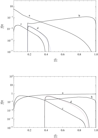
Figure 11: The dependence of the photon absorption rate in strong magnetic field ($B/B_{e}=200$) at temperatures 250 keV (upper panel) and 1 MeV (lower panel) for channels $\gamma_{2}\to\gamma_{1}\gamma_{1}$ – dotted line, $\gamma_{1}\gamma_{2}\to\gamma_{1}$ – ${\it a}$, $\gamma_{2}\gamma_{2}\to\gamma_{1}$ – ${\it b}$, $\gamma_{1}\gamma_{1}\to\gamma_{2}$ – ${\it c}$, $\gamma_{2}\gamma_{1}\to\gamma_{1}$ – ${\it d}$ on energy of the initial photon. Here, $\theta=\pi/2$.

$${\cal M}_{1\to 1}=\frac{8i\pi\alpha m}{eB}\,\frac{(q\varphi q^{\prime})(q\tilde{\varphi}q^{\prime})}{\sqrt{q^{2}_{\mbox{\tiny$\bot$}}q^{\prime 2}_{\mbox{\tiny$\bot$}}(-Q^{2}_{\mbox{\tiny$\|$}})}},$$ (73)

$${\cal M}_{1\to 2}=\frac{8i\pi\alpha m}{eB}\,\frac{(q\Lambda q^{\prime})(q^{\prime}\tilde{\Lambda}Q)}{\sqrt{q^{2}_{\mbox{\tiny$\bot$}}q^{\prime 2}_{\mbox{\tiny$\|$}}(-Q^{2}_{\mbox{\tiny$\|$}})}},$$ (74)

$${\cal M}_{2\to 1}=-\frac{8i\pi\alpha m}{eB}\,\frac{(q\Lambda q^{\prime})(q\tilde{\Lambda}Q)}{\sqrt{q^{2}_{\mbox{\tiny$\|$}}q^{\prime 2}_{\mbox{\tiny$\bot$}}(-Q^{2}_{\mbox{\tiny$\|$}})}},$$ (75)

$${\cal M}_{2\to 2}=16\pi\alpha m\,\frac{\sqrt{q^{2}_{\mbox{\tiny$\|$}}q^{\prime 2}_{\mbox{\tiny$\|$}}}\,\sqrt{(-Q^{2}_{\mbox{\tiny$\|$}})}\,\varkappa}{(q\tilde{\Lambda}q^{\prime})^{2}-\varkappa^{2}(q\tilde{\varphi}q^{\prime})^{2}}$$ (76)

$$\times\left\{1-\frac{q^{2}_{\mbox{\tiny$\bot$}}+q^{\prime 2}_{\mbox{\tiny$\bot$}}}{4eB}+i\frac{(q\varphi q^{\prime})(q\tilde{\varphi}q^{\prime})}{2eB\varkappa q^{2}_{\mbox{\tiny$\|$}}q^{\prime 2}_{\mbox{\tiny$\|$}}Q^{2}_{\mbox{\tiny$\|$}}}\right.$$

$$\times\left.\left[4m^{2}(q\tilde{\Lambda}q^{\prime})+(q\tilde{\Lambda}q^{\prime})^{2}-\varkappa^{2}(q\tilde{\varphi}q^{\prime})^{2}\right]\right\},$$

where $\varkappa=\sqrt{1-4m^{2}/Q^{2}_{\mbox{\tiny$\|$}}}$ and $Q^{2}_{\mbox{\tiny$\|$}}=(q-q^{\prime})^{2}_{\mbox{\tiny$\|$}}<0$, $q_{\alpha}=(\omega,{\bf k})$ and $q^{\prime}_{\alpha}=(\omega^{\prime},{\bf k^{\prime}})$ are the four-momentum of the initial and final photons correspondingly. From the last equation we can see that in the case, when the initial photon propagates across magnetic field direction, all amplitudes except ${\cal M}_{2\to 2}$ are suppressed by magnetic field strength. Therefore one could expect that mode 2 has the largest scattering absorption rate in this case. In turn, in the case when the initial photon propagates almost along ${\mathbb{B}}$, the amplitude ${\cal M}_{2\to 2}$ is suppressed by a small angle between photon momenta and magnetic field direction and becomes comparable to other amplitudes.

The general expression of the photon absorption rates is given by the formula RCh09 :

$$W_{\lambda e^{\pm}\to\lambda^{{}^{\prime}}e^{\pm}}=\frac{eB}{16(2\pi)^{4}\omega_{\lambda}}\int\mid{\cal M_{\lambda\to\lambda^{{}^{\prime}}}}\mid^{2}Z_{\lambda}Z_{\lambda^{{}^{\prime}}}$$

$$\times f_{\pm}(E)\,(1-f_{\pm}(E^{\prime}))(1+f_{\omega^{\prime}})$$ (77)

$$\times\delta(\omega_{\lambda}({\bf k})+E-\omega_{\lambda^{{}^{\prime}}}({\bf k^{\prime}})-E^{\prime})\frac{dp_{z}\,d^{3}k^{{}^{\prime}}}{EE^{\prime}\omega_{\lambda^{{}^{\prime}}}},$$

where $E=\sqrt{p_{z}^{2}+m^{2}}$ and $E^{\prime}=\sqrt{(p_{z}+k_{z}-k^{\prime}_{z})^{2}+m^{2}}$ are the energies of the initial and final electrons (positrons) correspondingly. In the case of the low-temperature limit ($T\ll m$) and neglecting the final photon distribution function $(f_{\omega^{\prime}}=0)$ absorption rates (77) can be expressed in terms of partial cross sections $W_{\lambda\to\lambda^{{}^{\prime}}}\equiv W_{\lambda e^{-}\to\lambda^{{}^{\prime}}e^{-}}+W_{\lambda e^{+}\to\lambda^{{}^{\prime}}e^{+}}\simeq n_{e}\sigma_{\lambda\to\lambda^{{}^{\prime}}}$

$$\sigma_{1\to 1}=\frac{3}{16}\,\sigma_{T}\left(\frac{B_{e}}{B}\right)^{2}\frac{\omega^{2}}{m^{2}}\,\left[\frac{(2m+\omega(1-u^{2}))(m+\omega+(m-\omega)u^{2})}{(\omega+m)^{2}-\omega^{2}u^{2}}\,+\frac{m}{\omega}(1-u^{2})\ln\left(\frac{(\omega+m)^{2}-\omega^{2}u^{2}}{m^{2}}\right)\right],$$ (78)

$$\sigma_{2\to 1}=\frac{3}{16}\,\sigma_{T}\left(\frac{B_{e}}{B}\right)^{2}\frac{q^{2}_{\mbox{\tiny$\bot$}}}{m^{2}\omega}\,Z_{2}\,\left[\frac{(2m\omega+q^{2}_{\mbox{\tiny$\|$}})(2m\omega^{2}-(m-\omega)q^{2}_{\mbox{\tiny$\|$}})(1-u^{2})}{q^{2}_{\mbox{\tiny$\|$}}[(\omega+m)^{2}(1-u^{2})-q^{2}_{\mbox{\tiny$\bot$}}u^{2}]}\,-m\ln\left(\frac{(\omega+m)^{2}(1-u^{2})-q^{2}_{\mbox{\tiny$\bot$}}u^{2}}{(1-u^{2})m^{2}}\right)\right],$$

$$q^{2}_{\mbox{\tiny$\|$}}=\omega^{2}-q^{2}_{\mbox{\tiny$\bot$}}u^{2}/(1-u^{2})$$ (79)

$$\sigma_{1\to 2}=\frac{3}{4}\,\sigma_{T}\left(\frac{B_{e}}{B}\right)^{2}\frac{1}{\omega s_{1\mbox{\tiny$\|$}}}\!\!\!\!\int\limits_{0}^{\,\,\,\,\,\,(m-\sqrt{s_{1\mbox{\tiny$\|$}}})^{2}\!/4m^{2}}\!\!\!\!\!\!\!dz\left(1+\frac{3}{2}\xi\,\frac{H(z)}{z}\right)\frac{(\omega+m)(s_{1\mbox{\tiny$\|$}}-m^{2})^{2}-4m^{2}z(m^{2}(\omega+m)+(\omega+3m)s_{\mbox{\tiny$\|$}})}{\sqrt{(s_{1\mbox{\tiny$\|$}}-m^{2}+4m^{2}z)^{2}-4m^{2}s_{1\mbox{\tiny$\|$}}z}},$$

$$s_{1\mbox{\tiny$\|$}} = (\omega+m)^{2}-\omega^{2}u^{2},$$ (80)

$$\sigma_{2\to 2} =3\,\sigma_{T}\,\frac{m}{\omega}\,Z_{2}\,\int\limits_{0}^{\,\,\,\,\,\,(\sqrt{s_{2\mbox{\tiny$\|$}}}-m)^{2}\!/4m^{2}}\!\!\!\!\!\!\!\frac{dz}{\sqrt{(s_{2\mbox{\tiny$\|$}}-m^{2}+4m^{2}z)^{2}-16m^{2}s_{2\mbox{\tiny$\|$}}z}}\times$$

$$\times \sum^{2}_{i=1}\frac{4m^{4}}{[(q\tilde{\Lambda}q^{\prime})^{2}-\varkappa^{2}(q\tilde{\varphi}q^{\prime})^{2}]^{2}}\bigg{[}4m^{2}q^{2}_{\mbox{\tiny$\|$}}z(4m^{2}-Q^{2}_{\mbox{\tiny$\|$}})\left(1-\frac{B_{e}}{B}\left(\frac{q^{2}_{\mbox{\tiny$\bot$}}}{4m^{2}}+z+\frac{3}{2}\xi\,H(z)\right)\right)^{2}+$$

$$+ \frac{1}{8m^{4}}\left(\frac{B_{e}}{B}\right)^{2}\,\frac{q^{2}_{\mbox{\tiny$\bot$}}(q\tilde{\varphi}q^{\prime})^{2}}{q^{2}_{\mbox{\tiny$\|$}}(-Q^{2}_{\mbox{\tiny$\|$}})}\,\left(1+\frac{3}{2}\xi\,\frac{H(z)}{z}\right)\,\left(4m^{2}(q\tilde{\Lambda}q^{\prime})+(q\tilde{\Lambda}q^{\prime})^{2}-\varkappa^{2}(q\tilde{\varphi}q^{\prime})^{2}\right)^{2}\bigg{]}_{\bigg{|}_{\,q^{\prime}_{z}=q^{\prime}_{zi}}\!\!\!\!\!\!\!\!\!\!\!\!\!\!\!\!\omega^{\prime}=\omega^{\prime}_{i}}$$

$$\omega^{\prime}_{1,2} = \frac{1}{2s_{2\mbox{\tiny$\|$}}}\left\{(\omega+m)(s_{2\mbox{\tiny$\|$}}-m^{2}+4m^{2}z)\pm\sqrt{q^{2}_{\mbox{\tiny$\bot$}}}\frac{u}{\sqrt{1-u^{2}}}\,\sqrt{(s_{2\mbox{\tiny$\|$}}-m^{2}+4m^{2}z)^{2}-4m^{2}s_{2\mbox{\tiny$\|$}}z}\right\},$$

$$q^{\prime}_{z1,2} = \frac{1}{2s_{2\mbox{\tiny$\|$}}}\left\{\sqrt{q^{2}_{\mbox{\tiny$\bot$}}}\frac{u}{\sqrt{1-u^{2}}}\,(s_{2\mbox{\tiny$\|$}}-m^{2}+4m^{2}z)\pm(\omega+m)\sqrt{(s_{2\mbox{\tiny$\|$}}-m^{2}+4m^{2}z)^{2}-4m^{2}s_{2\mbox{\tiny$\|$}}z}\right\},$$

$$s_{2\mbox{\tiny$\|$}} = (\omega+m)^{2}-q^{2}_{\mbox{\tiny$\bot$}}\frac{u^{2}}{1-u^{2}},$$

Figure 12: The dependence of the total photon absorption rate $W_{2\to 2}+W_{2\to 1}$ on energy of the initial photon in strong magnetic field $B/B_{e}\,=\,200$ at $T\,=\,1$ MeV – a and $T\,=\,50$ keV – b. The long dashed line c corresponds to the Compton scattering absorption rates without taking into account photon dispersion and wave function renormalization at $T\,=\,1$ MeV. Here, $\theta=\pi/2$.

where $\sigma_{T}=\frac{8\pi}{3}\frac{\alpha^{2}}{m^{2}}$ is the Thompson cross section, $\xi$ is the parameter defined in Sec. IV, $q^{2}_{\mbox{\tiny$\bot$}}$ is the root of equation $q^{2}_{\mbox{\tiny$\bot$}}=(1-u^{2})\,[\omega^{2}-{\cal P}^{(2)}(\omega^{2}-q^{2}_{\mbox{\tiny$\bot$}}u^{2}/(1-u^{2}))]$ and the number of electron (positron) density in a strongly magnetized and charge-symmetric rarefied plasma is defined by (56). To verify the result obtained we have calculated the corresponding cross sections in low-energy limit($\omega\ll m$):

$$\sigma_{1\to 1} \simeq \frac{3}{4}\,\sigma_{T}\left(\frac{B_{e}}{B}\right)^{2}\frac{\omega^{2}}{m^{2}},$$ (82)

$$\sigma_{1\to 2} \simeq \frac{1}{4}\,\sigma_{T}\left(\frac{B_{e}}{B}\right)^{2}\frac{\omega^{2}}{m^{2}}\,(1+\xi),$$ (83)

$$\sigma_{2\to 1} \simeq \frac{3}{4}\,\sigma_{T}\left(\frac{B_{e}}{B}\right)^{2}\frac{(\omega-\omega_{pl})^{2}}{m^{2}}\,(1+\xi)u^{2}\,\Theta(\omega-\omega_{pl}),$$

$$\sigma_{2\to 2} \simeq \frac{\sigma_{T}}{1+\xi}\bigg{\{}(1-u^{2})\left[1-\frac{1}{2}\,\left(\frac{B_{e}}{B}\right)\left(\frac{\omega}{m}\right)^{2}\left(\frac{9}{5}-u^{2}\right)\right]$$ (85)

$$+ \left(\frac{B_{e}}{B}\right)^{2}\frac{(\omega-\omega_{pl})^{2}}{4m^{2}}u^{2}\bigg{\}}\Theta(\omega-\omega_{pl}),$$

Figure 13: The dependence of the total photon absorption rate $W_{1\to 1}+W_{1\to 2}$ on energy of the initial photon in strong magnetic field $B/B_{e}\,=\,200$ at $T\,=\,1$ MeV – a and $T\,=\,50$ keV – b. The dashed-dotted line corresponds to the total probability of photon splitting $W_{1\to 12}+W_{1\to 22}$ at $T\,=\,50$ keV. Here, $\theta=\pi/2$.

One can see that the presence of magnetized plasma slightly influences on the process cross sections in this limit. Moreover, the corrections connected with photon dispersion and wave function renormalization are significant only for $\xi\sim 1$, i.e., when the magnetic field is rather strong $B\sim 10^{3}B_{e}$. In the case $\xi\ll 1$ which is relevant for the models of magnetar magnetosphere emission the formulas (82 – LABEL:eq:sigma21sT) coincide with the well-known result Herold:1979 . However, the cross section (85) contains the extra term $\sim B_{e}/B$ in comparison with result Herold:1979 . This term arises from the series expansion of exponents in the amplitude (71) (see also (76)) in terms of magnetic field strength.

For the numerical analysis of photon absorption rates under hot plasma conditions ($T\sim m$) it is convenient to make integration in (77) over $p_{z}$. Then for $W_{\lambda\to\lambda^{\prime}}$ we obtain the following simplified expression:

$$W_{\lambda\to\lambda^{\prime}}=\frac{eBZ_{\lambda}}{4(2\pi)^{4}\omega_{\lambda}}\int\frac{d^{3}k^{\prime}}{\varkappa|Q_{\mbox{\tiny$\|$}}^{2}|\omega_{\lambda^{\prime}}}\mid{\cal M_{\lambda\to\lambda^{{}^{\prime}}}}\mid^{2}Z_{\lambda^{\prime}}$$

$$\times(1+f_{\omega^{\prime}})\bigg{\{}{\cal F}_{5}\left[-\frac{1}{2T}(Q_{0}-Q_{z}\varkappa),\frac{1}{2T}(Q_{0}+Q_{z}\varkappa)\right]$$

$$\times\Theta(Q_{z})+(Q_{z}\to-Q_{z})\bigg{\}}\,,$$ (86)

where ${\cal F}_{5}(x,y)=[1+\exp{(x)}]^{-1}[1+\exp{(-y)}]^{-1}$.

The results of numerical calculations are presented in Figs. 12-15. In the Figs. 12 and 13 one can see that photon absorption rates corresponding to Compton scattering are the fast increasing functions of temperature. At the same time, the channels with initial photon of mode 1 and mode 2 have different character of the absorption coefficient energy dependence.

As shown in the Fig.12 the total absorption rate for the reactions $\gamma_{2}e^{\pm}\to\gamma_{2}e^{\pm}$ and $\gamma_{2}e^{\pm}\to\gamma_{1}e^{\pm}$ have threshold $(\omega=\omega_{pl})$. It is caused by mode 2 dispersion relation and indicates the fact that the electromagnetic wave corresponding to mode 2 cannot propagate with energy below $\omega_{pl}$.

Figure 14: The dependence of the absorption rates $W_{1\to 1}$ (upper panel) and $W_{2\to 2}$ (lower panel) on the angle between initial photon momentum and magnetic field direction at different initial photon energies ($B/B_{e}\,=\,200,T\,=\,1\mbox{MeV}$). The numbers above the curves correspond to the values of the ratio $\omega/2m$.

On the other hand, the electromagnetic wave, corresponding to the 2-mode quickly attenuates in the region $\omega\geqslant 2m$ due to the process $\gamma_{2}\to e^{+}e^{-}$. We would like to note that in the vicinity of the pair creation threshold taking into account the wave function renormalization and photon dispersion becomes very important and defines the processes rates’ dependencies on energy, temperature and magnetic field. It is well seen from the comparison of the solid and long dashed lines a and c (Fig. 12) calculated with and without taking into account photon dispersion and wave function renormalization, correspondingly.

The energy dependence of total rates $W_{1\to 1}+W_{1\to 2}$ is depicted in the Fig. 13. One can see the fast increase of absorption coefficients at low energies and rather slow dependence at $\omega\gtrsim 2m$. Such behavior indicates the possibility of the 1-mode photons efficient diffusion in the emission region whereas 2-mode seemed to be trapped.

Figure 15: The dependence of the absorption rates of the channels $W_{1\to 2}$ (upper panel) and $W_{2\to 1}$ (lower panel) on the angle between initial photon momentum and magnetic field direction at different initial photon energies ($B/B_{e}\,=\,200,T\,=\,1\mbox{MeV}$). The numbers above the curves correspond to the values of the ratio $\omega/2m$.

It is interesting also to consider the angle distributions of the photon absorption rates wasn’t analysed before in RCh09 (see Figs. 14 and 15). It is seen, that in the hot plasma the angle dependence of $W_{1\to 1}$ and $W_{1\to 2}$ is close to isotropic distribution. Recall, that in the low-temperature limit, the same angle distribution is strictly isotropic (see (82) and (83)). In contrast, the absorption rates $W_{2\to 1}$ and $W_{2\to 2}$ strongly depend on angle. They are minimized at $\theta=0$ and have maximum when 2-mode initial photon propagates across magnetic field direction.

VI Discussions

In the models of soft gamma repeaters spectrum formation the dependence of photon absorption rates on energy and temperature plays an important role. It could influence the shape of emergent spectrum and define the temperature profile in the emission region during bursts in SGRs Thompson:1995 ; Lyubarsky:2002 ; Thompson:2001 .

The previous investigations of the radiation transfer problem in strongly magnetized plasma have shown that along with the Compton scattering process the photon splitting $\gamma\to\gamma\gamma$ could play a significant role as a mechanism of photon production Thompson:1995 ; Thompson:2001 . In Sec. IV it was shown that at the temperature $T\sim m$ in kinematical region $\omega\leq 2m$ the main photon splitting process is $\gamma_{2}\to\gamma_{1}\gamma_{1}$ forbidden in pure magnetic field. However, the comparison of Fig. 8 and Fig. 12 shows that the rate of this process is much slower than the Compton scattering one $W_{2\to 1}+W_{2\to 2}$. Nevertheless, it could be an effective photon production mechanism at temperatures under consideration.

The total probability of the channels $\gamma_{1}\to\gamma_{1}\gamma_{2}$ and $\gamma_{1}\to\gamma_{2}\gamma_{2}$ increases with temperature falling and becomes comparable and even larger than the total Compton scattering rate $W_{1\to 1}+W_{1\to 2}$. As shown in Fig. 13 the process of photon splitting (dashed-dotted line) strongly dominates over Compton scattering at $T=50$ keV.

It was claimed previously that the effect of strongly magnetized cold plasma on photon splitting is not pronounced and the vacuum approximation can be used in the most calculations Bulik:1997 ; Elmfors:1998 . Our analysis shows that in the presence of hot plasma the process of photon splitting could be not only an intensive source of photon production but also an effective absorption mechanism.

Figure 16: The diffusion coefficient ${\cal D}_{1}=\omega^{2}W_{0}D_{1}/(2m)^{2}$, where $D_{1}$ is defined by (88), as a function of the ratio $\omega/2m$ at $T=1$ MeV and $B=200B_{e}$. The solid and long dashed lines correspond to diffusion coefficient with and without taking into account photon dispersion and wave function renormalization. The approximation (90) is depicted by the short dashed line.

Let us illustrate this fact in the framework of the magnetar model of SGR burst. It is known that the radiation transfer in the magnetically trapped plasma may be described as diffusion of the 1-mode photons whereas 2-mode photons are locked Thompson:1995 ; Lyubarsky:2002 ; Thompson:2001 . The last circumstance is connected especially with weak dependence of the 2-mode absorption coefficient on photon energy (see Fig. 13). We can approximatively describe the radiation transfer under the considered conditions via a diffusion equation (see for example Nagel ):

$$\frac{\partial n^{\omega}_{\lambda}}{\partial t}-\frac{\partial}{\partial z}\left(D_{\lambda}\frac{\partial n^{\omega}_{\lambda}}{\partial z}\right)=Q^{\omega}_{\lambda}\,,$$ (87)

where $n^{\omega}_{\lambda}$ is the photon number of density for $\lambda=1,2$ modes, $Q^{\omega}_{\lambda}$ is the source of $\lambda$-mode photon,

$$D_{\lambda}(\omega,z)=\int\frac{d\Omega}{4\pi}\ell_{\lambda}(\theta,\omega,z)\cos^{2}{\theta}\,$$ (88)

is the diffusion coefficient and $D_{1}\gg D_{2}$,

$$\ell_{\lambda}=\left[\,\sum\limits_{\lambda^{\prime}=1}^{2}W_{\lambda\to\lambda^{\prime}}+\sum\limits_{\lambda^{\prime},\lambda^{\prime\prime}=1}^{2}\left(W_{\lambda\to\lambda^{{}^{\prime}}\lambda^{{}^{\prime\prime}}}+W_{\lambda\lambda^{{}^{\prime}}\to\lambda^{{}^{\prime\prime}}}\right)\right]^{-1}\,$$ (89)

is the mode $\lambda$ photon free path.

Note that in the magnetar model of SGR burst Thompson:1995 ; Thompson:2001 in the analysis of radiation transfer Herold’s approximation of Compton scattering cross sections (82) and (83) was used. In this case the 1-mode photon free path can be written as

$$\ell_{1}^{H}=3D_{1}\simeq\frac{1}{n_{e}\sigma_{T}}\,\left(\frac{m}{\omega}\right)^{2}\left(\frac{B}{B_{e}}\right)^{2}\,.$$ (90)

In the Fig. 16 we demonstrate the importance of taking into account dispersion and wave function renormalization of photons in the radiation transfer problem. From the analysis above it follows that in the hot plasma $T\sim m$ the Compton scattering gives the main contribution to the photon free path and, as a consequence, to the diffusion coefficient. It is seen that photon dispersion and wave function renormalization become essential at initial photon energies, $\omega\gtrsim m$ (compare solid and long dashed lines in the Fig. 13). We can see also that approximation (90) is not applicable in hot plasma (dashed line).

Figure 17: The ratio $R=\ell_{1}/\ell_{1}^{H}$ as a function of the photon energy at $B=200B_{e}$

To demonstrate that the photon splitting process can be considered not only as the source of the photons but also as an effective absorption mechanism we depict the ratio of 1-mode photon free path (89) and approximation (90), $R=\ell_{1}/\ell_{1}^{H}$ at $T=50$ keV and $\theta=\pi/2$ (Fig. 17). It is seen that taking into account the photon splitting contribution leads to the essential increase of 1-mode photon free path in comparison to the commonly used approximation (90) in a wide range of photon energies.

The solution of the diffusion Eq. (87) is out of the scope of this article. However, we would like to note that the more detailed analysis of the radiation transfer needs the consistent solution of the Boltzmann equation for the photon occupation number and radiative transfer equation in the wide range of temperatures (10 keV $\lesssim T\lesssim$ 1 MeV).

VII Conclusions

In conclusion, we have investigated the influence of the strongly magnetized hot plasma on the photon splitting (merging) and Compton scattering processes taking into account the photon dispersion and large radiative corrections. The partial amplitudes and polarization selection rules for the process of photon splitting were obtained. The obtaining results show that plasma influence modifies the polarization selection rules in comparison to the pure magnetic field. In particular, the new splitting channel $\gamma_{2}\to\gamma_{1}\gamma_{1}$, forbidden without plasma, is allowed. On the other hand, the presence of plasma suppresses the probabilities of channels $\gamma_{1}\to\gamma_{1}\gamma_{2}$ and $\gamma_{1}\to\gamma_{2}\gamma_{2}$ in comparison to the pure magnetic field.

In addition, it was found that in hot plasma radiation transfer mainly occurs by means of 1-mode photon diffusion whereas the 2-mode is trapped. The comparison of the photon splitting (merging) processes and Compton scattering shows that the influences of these reactions on the 1-mode radiation transfer are competitive in rarefied plasma $(T\ll m)$. As a result, it could lead to the modification in the mechanism of the spectra formation of SGR and AXP.

Acknowledgements

We are grateful to N.V. Mikheev and A.V. Kuznetsov for stimulating discussions and valuable comments.

The study was performed within the State Assignment for Yaroslavl University Project No. 2.4176.2011, and was supported in part by the Russian Foundation for Basic Research Project No. 11-02-00394-a.

References

- (1) S. L. Adler, J. N. Bahcall, C. G. Callan, and M. N. Rosenbluth, Phys.Rev. Lett. 25, 1061 (1970).
- (2) Z. Bialynicka-Birula and L. I. Bialynicka-Birula, Phys. Rev. D2, 2341 (1970).
- (3) S. L. Adler, Ann. Phys. (N.Y.) 67, 599 (1971).
- (4) V. O. Papanian and V. I. Ritus, Sov. Phys. JETP 34, 1195 (1972).
- (5) R. J. Stoneham, J. Phys. A12, 2187 (1979).
- (6) M. Mentzel, D. Berg, and G. Wunner, Phys. Rev. D50, 1125 (1994); C. Wilke and G. Wunner, D55, 997 (1997).
- (7) S. L. Adler and C. Schubert, Phys. Rev. Lett. 77, 1695 (1996).
- (8) V. N. Baier, A. I. Milstein and R. Zh. Shaisultanov, Phys. Rev. Lett. 77, 1691 (1996).
- (9) M. V. Chistyakov, A. V. Kuznetsov and N. V. Mikheev, Phys.Lett. B434, 67 (1998); A. V. Kuznetsov, N. V. Mikheev and M. V. Chistyakov, Yad. Fiz. 62, 1638 (1999) [Phys. At. Nucl. 62, 1535 (1999)].
- (10) J. I. Weise, Phys. Rev. D69, 105017 (2004).
- (11) V. O. Papanian and V. I. Ritus, Issues in Intense-Field Quantum Electrodynamics, ed. by V.L. Ginzburg (Nova Science Publishers, New York, 1989), pp. 153-179.
- (12) A. K. Harding and D. Lai, Rep.Prog.Phys. 69, 2631 (2006).
- (13) A. K. Harding, M. G. Baring and P. L. Gonthier, Astrophys.J. 476, 246 (1997).
- (14) R. C. Duncan and C. Thompson, Astrophys. J. 392, L9 (1992).
- (15) M. G. Baring, Astrophys. J. 440, L69 (1995).
- (16) C. Thompson and R. C. Duncan, Mon. Not. Roy. Astron. Soc. 275, 255 (1995).
- (17) M. G. Baring and A. K. Harding, Astrophys. J. Lett. 507, L55 (1998).
- (18) V. M. Malofeev, O. I. Malov, D. A. Teplykh, S.A. Tyul bashev, and G. E. Tyul basheva, Astronomy Reports 49, 242 (2005).
- (19) Y. N. Istomin and D. N. Sobyanin, Astron. Lett., 33, 660 (2007).
- (20) C. Thompson and R. C. Duncan, Astrophys. J. 561, 980 (2001).
- (21) T. Bulik, Acta Astronomica. 48, 695 (1998).
- (22) P. Elmfors and B. Skagerstam, Phys. Lett. B427, 197 (1998).
- (23) H. Gies, Phys. Rev. D61, 085021 (2000).
- (24) J. M. Martinez Resco and M. A. Valle Basagoiti, Phys. Rev. D64, 016006 (2001).
- (25) H. Herold, Phys. Rev. D19, 2868 (1979).
- (26) D.B. Melrose and A.J. Parle, Aust. J. Phys. 36, 799 (1983).
- (27) J.K. Daugherty and A.K. Harding, Astrophys. J. 309, 362 (1986).
- (28) P.L. Gonthier, A.K. Harding, M.G. Baring et al., Astrophys. J. 540, 907 (2000).
- (29) T. Bulik and M.C. Miller, Mon. Not. R. Astron. Soc. 288, 596 (1997).
- (30) A. V. Kuznetsov and N. V. Mikheev, JETP 91, 748 (2000).
- (31) D. A. Rumyantsev and M. V. Chistyakov, JETP 101, 635 (2005).
- (32) M. V. Chistyakov and N. V. Mikheev, Mod.Phys.Lett. A17, 2553 (2002).
- (33) E. S. Fradkin, Tr. Fiz. Inst. Akad.Nauk SSSR 29, 7 (1965).
- (34) H. A. Weldon, Phys. Rev. D 26, 1394 (1982).
- (35) A. E. Shabad, Tr. Fiz. Inst. Akad. Nauk SSSR 192, 5 (1988).
- (36) H. Pérez Rojas and A. E. Shabad, Ann. Phys. (N.Y.) 121, 432 (1979).
- (37) H. Pérez Rojas and A. E. Shabad, Ann. Phys. (N.Y.) 138, 1 (1982).
- (38) A. E. Shabad, V. V. Usov, Sov. Astron. Lett. 9,212 (1983).
- (39) V. V. Usov, Astrophys. J., 572, L87 (2002).
- (40) D. A. Rumyantsev and M. V. Chistyakov, Int. J. Mod. Phys. A 24, 3995 (2009).
- (41) A. Chodos, K. Everding and D. A. Owen, Phys. Rev. D42, 2881 (1990).
- (42) A. V. Kuznetsov and A. A. Okrugin, Int. J. Mod. Phys. A26, 2725 (2011).
- (43) Y. E. Lyubarsky, Mon. Not. R. Astron. Soc. 332, 199 (2002).
- (44) W. Nagel, Astrophys.J. 236, 904 (1980).