Taylor–Socolar Hexagonal Tilings As Model Sets

Abstract.

The Taylor–Socolar tilings [19, 20] are regular hexagonal tilings of the plane but are distinguished in being comprised of hexagons of two colors in an aperiodic way. We place the Taylor–Socolar tilings into an algebraic setting which allows one to see them directly as model sets and to understand the corresponding tiling hull along with its generic and singular parts.

Although the tilings were originally obtained by matching rules and by substitution, our approach sets the tilings into the framework of a cut and project scheme and studies how the tilings relate to the corresponding internal space. The centers of the entire set of tiles of one tiling form a lattice $Q$ in the plane. If $X_{Q}$ denotes the set of all Taylor–Socolar tilings with centers on $Q$ then $X_{Q}$ forms a natural hull under the standard local topology of hulls and is a dynamical system for the action of $Q$. The $Q$-adic completion $\overline{Q}$ of $Q$ is a natural factor of $X_{Q}$ and the natural mapping $X_{Q}\longrightarrow\overline{Q}$ is bijective except at a dense set of points of measure $0$ in $\overline{Q}$. We show that $X_{Q}$ consists of three LI classes under translation. Two of these LI classes are very small, namely countable $Q$-orbits in $X_{Q}$. The other is a minimal dynamical system which maps surjectively to $\overline{Q}$ and which is variously $2:1$, $6:1$, and $12:1$ at the singular points.

We further develop the formula of [19] that determines the parity of the tiles of a tiling in terms of the co-ordinates of its tile centers. Finally we show that the hull of the parity tilings can be identified with the hull $X_{Q}$; more precisely the two hulls are mutually locally derivable.

1. Introduction

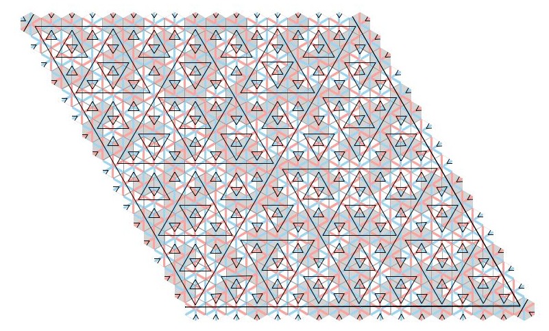
Figure 8. The figure shows a pattern of triangles emerging from the construction indicated in §2, manifesting the rule R1. The underlying hexagonal tiling is indicated in light and dark shades which indicate the parity of the hexagons. The underlying diagonal shading on the hexagons manifests the rules R2.

This paper concerns the aperiodic hexagonal mono-tilings created by Joan Taylor. We learned about these tilings from the unpublished (but available online) paper of Joan Taylor [20], the extended paper of Socolar and Taylor [19], and a talk given by Uwe Grimm at the KIAS conference on aperiodic order in September, 2010 [4]. These tilings are in essence regular hexagonal tilings of the plane, but there are two forms of marking on the hexagonal tile (or if one prefers, the two sides of the tile are marked differently). We refer to this difference as parity (and eventually distinguish the two sides as being sides $0$ and $1$), and in terms of parity the tilings are aperiodic. In fact the parity patterns of tiles created in this way are fascinating in their apparent complexity, see Fig. 1 and Fig. 8.

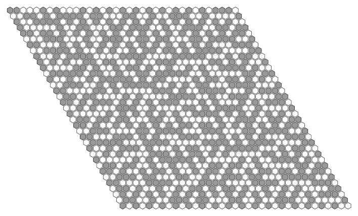
Figure 1. A section of a Taylor–Socolar tiling showing the complex patterning arising from the two sides of the hexagonal tile, here indicated in white and gray. Notice that there are islands (Taylor and Socolar call the llamas) both of white and gray tiles.

The two Taylor–Socolar tiles are shown in Fig. 2, the main features being the black lines, one of which is a stripe across the tile, and the three colored diameters, one of which is split in color. The difference in the two tiles is only in which side of the color-split diameter the stripe crosses. In the figure the tiles are colored white and gray to distinguish them, but it is the crossing-color of the black stripe that is the important distinguishing feature.

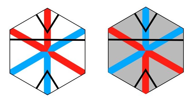
Figure 2. The two basic hexagonal tiles. One is a white tile and the other a light gray. These are colored with red and blue diameters. The rotational position of the tiles is immaterial. Note how the tiles are identical as far as the red diagonal and blue diagonal are concerned. The distinction is in which color of the red-blue diagonal cuts the black stripe.

Taylor–Socolar tilings can be defined by following simple matching rules (R1, R2) and can also be constructed by substitution (the scaling factor being $2$). In this paper it is the matching rules that are of importance.

• the black lines must join continuously when tiles abut;

• the ends of the diameters of two hexagonal tiles that are separated by an edge of another tile must be of opposite colors, Fig. 3.

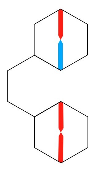
Figure 3. Rule R2: two hexagon tiles separated by the edge of another hexagon tile. Note that the diameter colors of the two hexagons are opposite at the two ends of the separating edge. It makes no difference whether or not the diameters are color-split – the diameters must have different colors where they abut the separating edge.

The paper [19] emphasizes the tilings from the point of view of matching rules, whereas [20] emphasizes substitution (and the half-hex approach). There is a slight mis-match between the two approaches, see [4], which we will discuss later.

If one looks at part of a tiling with the full markings of the tiles made visible, then one is immediately struck by how the black line markings of the tiles assemble to form nested equilateral triangles, see Fig. 8. Although these triangles are slightly shrunken (which ultimately is important), we see that basically the vertices of the triangles are tied to the centers of the hexagons, and the triangle side-lengths are $1,2,4,8,\dots$ in suitable units. This triangle pattern is highly reminiscent of the square patterns that underlie the famous Robinson tilings [17, 10] which also appear in sizes which scale up by factors of $2$. These tilings are limit-periodic tilings and can be described by model sets whose internal spaces are $2$-adic spaces. The Taylor-Socolar tilings are also limit-periodic and it seems natural to associate some sort of $2$-adic spaces with them and to give a model-set interpretation of the picture.

One purpose of this paper is to do this, and it has the natural consequence that the tilings are pure point diffractive. It is convenient to base the entire study on a fixed standard hexagonal tiling of the coordinate plane $\mathbb{R}\hskip 0.5pt^{2}$. The centers of the hexagonal tiles can then be interpreted as a lattice in the plane (with one center at $(0,0)$). The internal space of the cut and project scheme that we shall construct is based on a $2$-adic completion $\overline{Q}$ of the group $Q$ consisting of all translation vectors between the centers of the hexagons. We shall show that there is a precise one-to-one correspondence between triangulations and elements of $\overline{Q}$. But the triangulation is not the whole story.

The set of all Taylor–Socolar tilings associated with a fixed standard hexagonal tiling of the plane form a tiling hull $X_{Q}$. This hull is a dynamical system (with group $Q$) and carries the standard topology of tiling hulls. Each tiling has an associated triangulation, but the mapping $\xi:X_{Q}\longrightarrow\overline{Q}$ so formed, while generically $1-1$, is not globally $1-1$. What lies behind this is the question of backing up from the triangulations to the actual tilings themselves. The question is how are the tile markings deduced from the triangulations so as to satisfy the rules R1, R2? There are two aspects to this. The triangulations themselves are based on hexagon centers, whereas in an actual tiling the triangles are shrunken away from vertices. This shrinking moves the triangle edges and is responsible for the off-centeredness of the black stripe on each hexagon tile. How is this shrinking (or edge shifting, as we call it) carried out? The second feature is the coloring of the diagonals of the hexagons. What freedom for coloring exists, given that the coloring rule R2 must hold?

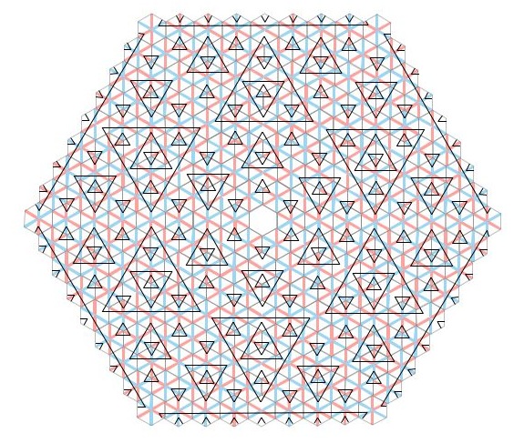
Figure 17. The (central part of a) central hexagon (CHT) tiling. Full (edge-shifted) triangles of levels $0,1,2$ are shown. At the outside edges one can see the beginnings of triangles of level $3$. The rays from the central hexagon in the six $a$-directions will have infinite $a$-lines in them. However the edge shifting rules cannot be applied to them because they are of infinite level – they are not composed of edges of finite triangles. In the end a full tiling is obtained by placing a fully decorated tile into the empty central hexagon. There are $12$ ways to do this, and each way then determines the rest of the tiling completely. These tilings violate both forms of generic condition.

In this paper we explain this and give a complete description of the hull and the mapping $\xi$, Theorem 6.9. There are numerous places at which $\xi$ is singular (not bijective); in fact the set of singular points in $\overline{Q}$ is dense. Two special classes of singular points are those corresponding to the central hexagon triangulations (CHT)(see Fig. 17) and the infinite concurrent $w$-line tilings (iCw-L) (see Fig. 18). In both cases there is $3$-fold rotational symmetry of the triangulation and in both cases the mapping $\xi$ is many-to-one. These two types of tilings play a significant role in [19].

The hull has a minimal invariant component of full measure and this is a single LI class. There are two additional orbits, whose origins are the iCw-L triangulations, and although they perfectly obey the matching rules they are not in the same LI class as all the other tilings. On the other hand the CHT tilings (those lying over the CHT triangulations) are in the main LI class and, because of the particular simplicity of the unique one whose center is $(0,0)$, the question of describing the parity (which tiles are facing up and which are facing down) becomes particularly easy. Here we reproduce the parity formula for this CHT tiling as given in [19] (with some minor modifications in notation). We use this to give parity formulas for all the tilings of $X_{Q}$.

A couple of comments about earlier work on aperiodic hexagonal tilings are appropriate here. D. Frettlöh [8] discusses the half-hex tilings (created out of a simple substitution rule) and proves that natural point sets associated with these can be expressed as model sets. Half-hexes don’t play an explicit role in this paper, though the hull of the half-hex tilings is a natural factor of $X_{Q}$ lying between $X_{Q}$ and $\overline{Q}$ [8, 9, 11]. They were important to Taylor’s descriptions of her tilings and are implicitly embedded in them.

In [15], Roger Penrose gives a fine introduction to aperiodic tilings and then goes on to create a class of aperiodic hexagonal tilings, which he calls $1+\epsilon+\epsilon^{2}$-tilings in which there are three types of tiles that assemble by matching rules. The main tiles are hexagonal, with keyed edges. The other two are a linear-like tile with an arbitrarily small width ($\epsilon$ tiles) which fit along the hexagon edges, and some very tiny tiles ($\epsilon^{2}$) which fit at the corners of the tiles.

Clearly his objective was to create a single tile that only tiles aperiodically, although that was not achieved in [15]. Subsequently, however, Penrose did find a solution to the problem that uses a single hexagonal tile with matching rules for the edges and corners, [16]. This has only recently become more widely known after Joan Taylor’s work started to circulate.

One can quibble about whether or not Taylor’s tiling stretches the concept of matching rules since the second rule relates non-adjacent tiles and also in her tiling there are two tiles, though (at least in the right markings) they are mirror images of each other. However, the tilings of Penrose and Taylor tilings are a fascinating pair. Extensive computational work of F. Gähler indicates that the two tilings are quite distinct from one another, though they both have $\overline{Q}$ as a factor and apparently both have the same dynamical zeta functions [3].

There is an algorithmic computation for determining that certain classes of substitution tilings have pure-point spectrum. It has been used to confirm that the Taylor–Socolar substitution tilings have pure point spectrum or, equivalently, are regular model sets [2].

2. The triangulation

In principle the tilings that we are interested in are not connected to the points of lattices and their cosets in $\mathbb{R}\hskip 0.5pt^{2}$, but are only point sets that arise in Euclidean space $\mathbb{E}$ as the vertices and centers of tilings. However, our objective here to realize tiling vertices in an algebraic context and for that we need to fix an origin and a coordinate system so as to reduce the language to that of $\mathbb{R}\hskip 0.5pt^{2}$. Let $Q$ be the triangular lattice in $\mathbb{R}\hskip 0.5pt^{2}$ defined by

$$Q:=\mathbb{Z}a_{1}+\mathbb{Z}a_{2}$$

where $a_{1}=(1,0)$ and $a_{2}=(-\frac{1}{2},\frac{\sqrt{3}}{2})$. Then $P:=\mathbb{Z}w_{1}+\mathbb{Z}w_{2}$ where $w_{1}=\frac{2}{3}a_{1}+\frac{1}{3}a_{2}$ and $w_{2}=\frac{1}{3}a_{1}+\frac{2}{3}a_{2}$ is a lattice containing $Q$ as sublattice of index $3$, see Fig. 4. For future reference we note that $|a_{1}|=|a_{2}|=|a_{1}+a_{2}|=1$ and $|w_{1}|=|w_{2}|=|w_{2}-w_{1}|=1/\sqrt{3}$.

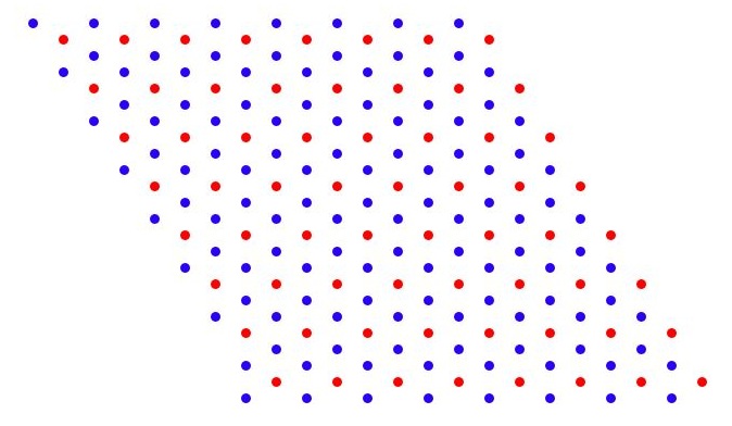
Figure 4. The figure shows the standard triangular lattice $Q$ (the red points) and the larger lattice $P$ (red and blue points) in which $Q$ lies with index $3$. The points of $Q$ may be viewed as the vertices of a triangularization of the plane by equilateral triangles of side length $1$. The red points are the centres of these triangles. The color here has nothing to do with the coloring of the diagonals of the tiles – it only distinguishes the two cosets.

Joining the points of $Q$ that lie at distance $1$ from one another creates a triangular tiling. Inside each of the unit triangles so formed there lies a point of $P$, and indeed $P$ consists of three $Q$ cosets: $Q$ itself, the centroids of the “up” triangles (those with a vertex above a horizontal edge), and the “down” triangles (those with a vertex below a horizontal edge), see Fig. 5. What we aim to do is to create a hexagonal tiling of $\mathbb{R}\hskip 0.5pt^{2}$. When this tiling is complete, the points of $Q$ will be the centers of the hexagonal tiles and the points of $P$ immediately surrounding the points of $Q$ will make up the vertices of the tiles.

Each of the hexagonal tiles will be marked by colored diagonals and a black stripe, see Fig. 2. These markings divide the tiles into two basic types, and it is describing the pattern made from these two types in model-set theoretical terms that is a primary objective of this paper (see Fig. 8). The other objective is to describe the dynamical hull that encompasses all the tilings that belong to the Taylor–Socolar tiling family.

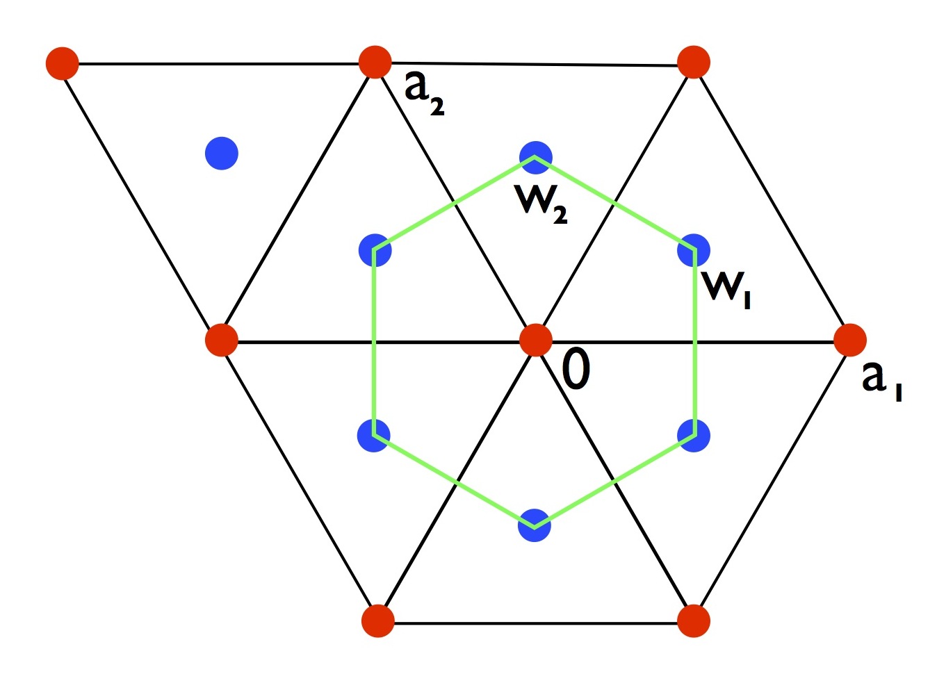
Figure 5. The generators $a_{1},a_{2}$ of $Q$ and the generators $w_{1},w_{2}$ of $P$, showing how the cosets of $Q$ in $P$ split into the points of $Q$ and the centroids (centers) of the up and down triangles. Around the point $0\in Q$ we see the hexagonal tile centered on $0$ with vertices in $P\backslash Q$.

We let the coset of up (respectively down) points be denoted by $S^{\uparrow}_{1}=w_{1}+Q$ and $S^{\downarrow}_{1}=w_{2}+Q$ respectively:

$$P=Q\cup S^{\uparrow}_{1}\cup S^{\downarrow}_{1}\,.$$

Remark 2.1.

There are three cosets of $Q$ in $P$. In our construction of the triangle patterns we have taken the point of view that $Q$ itself will be used for triangle vertices and the other two cosets for triangle centroids. However, we could use any of the three cosets as the triangle vertices and arrive at a similar situation. This amounts to a translation of the plane by $w_{1}$ or $w_{2}$. We come back to this point in §9.

We now wish to re-triangularize the plane still using points of $Q$ as vertices, but this time making triangles of side length equal to $2$ using as vertices a coset of $2Q$ in $Q$. There are four cosets of $2Q$ in $Q$ and they lead to four different ways to make the triangularization. Fig. 6 shows the four types of triangles of side length $2$. The lattices generated by the points of any one of these triangles is a coset of $2Q$ and together they make up all four cosets of $2Q$ in $Q$.

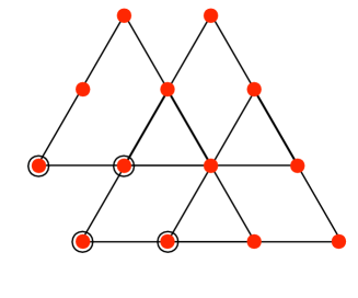
Figure 6. Four superimposed triangles, each indicated by its circled bottom lefthand vertex. The vertices of each triangle generate a different coset of $Q$ modulo $2Q$.

Choose one of these cosets, call it $q_{1}+2Q$, where $q_{1}\in Q$, and thereby triangulate the plane with triangles of side length $2$. The centroids of the new triangles are a subset of the original set of centroids and, in fact, together with the vertices $q_{1}+2Q$ they form the coset $q_{1}+2P$. This is explained in the Fig. 7, which also explains the important fact that the new centroids, namely those of the new edge-length-$2$ triangles of $q_{1}+2Q$, make up two cosets of $2Q$ in $q_{1}+2P$ depending on the orientation of the new triangles, and these orientations are opposite to those that these points originally had. Thus we obtain $S^{\uparrow}_{2}=q_{1}+2w_{1}+2Q$ (which is in $w_{2}+Q$  !), $S^{\downarrow}_{2}=q_{1}+2w_{2}+2Q$ (which is in $w_{1}+Q$), and the coset decomposition

$$q_{1}+2P=(q_{1}+2Q)\cup S^{\uparrow}_{2}\cup S^{\downarrow}_{2}\,$$

with $S^{\uparrow}_{2}\subset S^{\downarrow}_{1}$ and $S^{\downarrow}_{2}\subset S^{\uparrow}_{1}$.

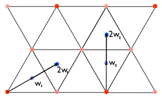
Figure 7. The figure shows how the centroids (indicated with solid blue dots) of the new side-length-$2$ triangles (indicated with solid red dots) are obtained as vectors from $q_{1}+2P$. The two $2Q$-cosets of $q_{1}+2P$ which are not $q_{1}+2Q$ itself indicate the centroids of the new up and down triangles. Notice that the orientations of the new triangles, and hence the orientations associated with the new centroids, are opposite to the orientations associated with these points when they were viewed as centroids of the original triangulation. This explains why $S^{\uparrow}_{2}\subset S^{\downarrow}_{1}$ and $S^{\downarrow}_{2}\subset S^{\uparrow}_{1}$ .

We now repeat this whole process. There are four cosets of $4Q$ in $q_{1}+2Q$ and we select one of them, say $q_{1}+q_{2}+4Q$, with $q_{2}\in 2Q$, and this gives us a new triangulation with triangles of side length $4$. Their centroids in $q_{1}+q_{2}+4P$ form $4Q$-cosets $S^{\uparrow}_{3}\subset S^{\downarrow}_{2}$ and $S^{\downarrow}_{3}\subset S^{\uparrow}_{2}$, and we have the decomposition

$$q_{1}+q_{2}+4P=(q_{1}+q_{2}+4Q)\cup S^{\uparrow}_{3}\cup S^{\downarrow}_{3}\,.$$

Continuing this way we obtain $q_{1},q_{2},q_{3},\dots$ with $q_{k}\in 2^{k-1}Q$, and sets $S^{\uparrow}_{k},S^{\downarrow}_{k}$ with $S^{\uparrow}_{k+1}\subset S^{\downarrow}_{k}$ and $S^{\downarrow}_{k+1}\subset S^{\uparrow}_{k}$ for all $k=1,2,\dots$, and the partition

(1) $$q_{1}+\cdots+q_{k}+2^{k}P=(q_{1}+\cdots+q_{k}+2^{k}Q)\cup S^{\uparrow}_{k+1}\cup S^{\downarrow}_{k+1}\,.$$

We have

(2) $$S^{\uparrow}_{k+1} = q_{1}+\cdots+q_{k}+2^{k}(w_{1}+Q)$$

$$S^{\downarrow}_{k+1} = q_{1}+\cdots+q_{k}+2^{k}(w_{2}+Q)\,.$$

Explicit formulas for $2^{k}w_{1}$ and $2^{k}w_{2}$ are given in Lemma 3.2.

We now carry out the entire construction based on an arbitrary infinite sequence

$$(q_{1},q_{2},\dots,q_{k},\dots)$$

where $q_{k}\in 2^{k-1}Q$ for all $k$. This results in a pattern of overlapping triangulations based on triangles of edge lengths $1,2,4,8,\dots$ (these are referred to as being triangles of levels $0,1,2,3,...$). In §4 we shall make our tiling out of this pattern. But certain features of the entire pattern are clear:

• all points involved as vertices of triangles are in $Q$;

• all triangle centroids are in $P\backslash Q$;

• there is no translational symmetry.

The last of these is due to the fact that there are triangles of all scales, and no translation can respect all of these scales simultaneously.

A point $x\in P\backslash Q$ is said to have an orientation (up or down) if there is a positive integer $k$ such that for all $k^{\prime}>k$, $x\notin S^{\uparrow}_{k^{\prime}}\cup S^{\downarrow}_{k^{\prime}}$. Every element of $P\backslash Q$ is in $S^{\uparrow}_{k}$ or $S^{\downarrow}_{k}$ for $k=1$, and some for other values of $k$ as well. For the elements $x$ which have an orientation there is a largest $k$ for which this is true and this gives its final orientation. If $x$ has an orientation, we shall say that the level of its orientation is $k$ if its orientation stabilizes at $k$. If it does not stabilize we shall say that $x$ is not oriented. We shall see below (Prop.  3.3) what it means for a point not to have an orientation.

3. The $Q$-adic completion

In this section we create and study a completion of $P$ under the $Q$-adic topology. The $Q$-adic topology is the uniform topology based on the metric on $P$ defined by $d(x,y)=2^{-k}$ if $x-y\in 2^{k}Q\backslash 2^{k+1}Q$ and $d(x,y):=2$ when $x,y$ are in different cosets of $Q$. This metric is $Q$-translation invariant. $\overline{P}$ is the completion of $P$ in this topology and $\overline{Q}$ is the closure of $Q$ in $\overline{P}$, which is also the completion of $Q$ in the $Q$-adic topology.

$\overline{P}$ may be viewed as the set of sequences

$$(b_{1},b_{2},\dots)$$

where $b_{k}\in P$ for all $k$ and $b_{k+1}\equiv b_{k}\mod 2^{k}Q$.

$\overline{P}$ is a group under component-wise addition and $\overline{Q}$ is the subgroup of all such sequences with all components in $Q$. There is the obvious coset decomposition

$$\overline{P}=\overline{Q}\cup(w_{1}+\overline{Q})\cup(w_{2}+\overline{Q})\,,$$

so $\overline{Q}$ has index $3$ in $\overline{P}$. We note that $\overline{Q}$ and $\overline{P}$ are compact topological groups.

We have $i:P\longrightarrow\overline{P}$ via

$$b\mapsto(b,b,b,\dots)\,.$$

We often identify $P$ as a subgroup of $\overline{P}$ via the embedding $i$.

Note that the construction of expanding triangles of §2 depends on the choice of the element $(q_{1},q_{2},\dots)$, where $q_{k}\in 2^{k-1}Q$. Then we can obtain the compatible sequence

$${\bf q}=(q_{1},q_{1}+q_{2},\dots,q_{1}+q_{2}+\cdots+q_{k},\dots)\in\overline{Q}$$

and thus we can identify each possible construction with an element of $\overline{Q}$. Let $\mathcal{T}({\bf q})$ denote the pattern of triangles arising from ${\bf q}\in\overline{Q}$.

Let $\mu$ denote the unique Haar measure on $\overline{P}$ for which $\mu(\overline{P})=1$. The key feature of $\mu$ is that $\mu(p+2^{k}\overline{Q})=2^{-k}/3$ for all $p\in\overline{P}$. We note that $P\subset\overline{P}$ is countable and has measure $0$, and that $\mu(\overline{Q})=\frac{1}{3}$ and $\mu(\overline{S^{\uparrow}_{k}})=\mu(\overline{S^{\downarrow}_{k}})=2^{-k+1}/3$.

Remark 3.1.

We should note a subtle point here. In $\overline{Q}$ one can divide by $3$. In fact, for all ${\bf x}\in\overline{Q}$, $-\lim_{k\to\infty}({\bf x}+4{\bf x}+4^{2}{\bf x}+\dots+4^{k}{\bf x})$ exists since $4^{k}{\bf x}\in 2^{2k}\overline{Q}$, and

$$-3\lim_{k\to\infty}({\bf x}+4{\bf x}+4^{2}{\bf x}+\dots+4^{k}{\bf x})=\lim_{k\to\infty}(1-4)({\bf x}+4{\bf x}+4^{2}{\bf x}+\dots+4^{k}{\bf x})=\lim_{k\to\infty}(1-4^{k+1}){\bf x}={\bf x}\,.$$

Thus we can find an element ${\bf w_{1}}$ of $\overline{Q}$ corresponding to $w_{1}=\frac{2}{3}a_{1}+\frac{1}{3}a_{2}$ and similarly ${\bf w_{2}}\in\overline{Q}$ corresponding to $w_{2}$ . However, our view is that $P=Q\cup(w_{1}+Q)\cup(w_{2}+Q)$ and $\overline{P}$ is the $Q$-adic completion of this, with each of the three cosets leading to a different coset of $\overline{Q}$ in $\overline{P}$. Thus $w_{1}-{\bf w_{1}}\neq 0$ but $3(w_{1}-{\bf w_{1}})=0$ and we conclude that $\overline{P}$ has $3$-torsion.

Two examples of this are important in what follows. Define $s_{1}^{(-1)}:=0$ and $s_{1}^{(k)}:=a_{1}+4a_{1}+4^{2}a_{1}+\cdots+4^{k}a_{1})$ for $k=0,1,\dots$. and similarly $s_{2}^{(k)}$ based on $a_{2}$. Their limits are denoted by ${\bf s_{1}},{\bf s_{2}}$ respectively. They lie in $\overline{Q}$.

Lemma 3.2.

For all $k=0,1,\dots$,

$$2^{2k}w_{1} = w_{1}+s_{2}^{(k-1)}+2s_{1}^{(k-1)}$$

$$2^{2k+1}w_{1} = w_{2}+s_{1}^{(k)}+2s_{2}^{(k-1)}\,.$$

Similarly for $2^{m}w_{2}$, interchanging the indices $1,2$.

In particular $\lim_{k\to\infty}2^{2k}w_{1}=w_{1}+{\bf s_{2}}+2{\bf s_{1}}$ and $\lim_{k\to\infty}2^{2k+1}w_{1}=w_{2}+{\bf s_{1}}+2{\bf s_{2}}$. Furthermore, $3(w_{1}+{\bf s_{2}}+2{\bf s_{1}})=0=3(w_{2}+{\bf s_{1}}+2{\bf s_{2}})$.

Proof.

From the definitions, $2w_{1}=w_{2}+a_{1}$ and $2w_{2}=w_{1}+a_{2}$. This gives the case $k=0$ of the Lemma. Now proceeding by induction,

$$2^{2k}w_{1}=2(w_{2}+s_{1}^{(k-1)}+2s_{2}^{(k-2)})=w_{1}+a_{2}+2s_{1}^{(k-1)}+4s_{2}^{(k-2)}=w_{1}+s_{2}^{(k-1)}+2s_{1}^{(k-1)}\,,$$

as required. Similarly

$$2^{2k+1}w_{1}=2(w_{1}+s_{2}^{(k-1)}+2s_{1}^{(k-1)})=w_{2}+a_{1}+2s_{2}^{(k-1)}+4s_{1}^{(k-1)}=w_{2}+s_{1}^{(k)}+2s_{2}^{(k-1)}\,.$$

Taking the limits and using the formula for multiplication by $3$ at the beginning of Remark 3.1, we find that $-3({\bf s_{2}}+2{\bf s_{1}})=a_{2}+2a_{1}=3w_{1}$ and similarly with the indices $1,2$ interchanged. ∎

Consider what happens if there is a point $x\in P\backslash Q$ which does not have orientation. This means that there is an infinite sequence $k_{1}<k_{2}<\cdots$ with $x\in S^{\uparrow}_{k_{j}}\cup S^{\downarrow}_{k_{j}}$. Then from (2), $x\in\left((q_{1}+\cdots+q_{k_{j}-1}+2^{k_{j}-1}(w_{1}+Q)\right)\cup\left((q_{1}+\cdots+q_{k_{j}-1}+2^{k_{j}-1}(w_{2}+Q)\right)$ for each $k_{j}$. This means $x={\bf q}+w_{1}+{\bf s_{2}}+2{\bf s_{1}}$ or $x={\bf q}+w_{2}+{\bf s_{1}}+2{\bf s_{2}}$.

Proposition 3.3.

$\mathcal{T}({\bf q})$ has at most one point without orientation. A point without orientation can occur if and only if ${\bf q}\in-{\bf s_{2}}-2{\bf s_{1}}+Q$ or ${\bf q}\in-{\bf s_{1}}-2{\bf s_{2}}+Q$. These two families are countable and disjoint.

Proof.

If $x\in P\backslash Q$ does not have an orientation then either $x={\bf q}+w_{1}+{\bf s_{2}}+2{\bf s_{1}}$ and $-w_{1}+x\in Q$, which gives one of the cases; or $x={\bf q}+w_{2}+{\bf s_{1}}+2{\bf s_{2}}$, which gives the other. Conversely, in either case we have points without orientation. Since in one case $x\in w_{1}+Q$ and in the other case $x\in w_{2}+Q$, we see that the two families are disjoint. ∎

Remark 3.4.

We do not need to go into the exact description of the orientations of triangles, but confine ourselves to a few remarks here. For any fixed ${\bf q}$, define the sequence of sets $W^{\uparrow}_{k}$ and $W^{\downarrow}_{k}$, $k=1,2,\dots$, inductively by $W^{\uparrow}_{1}=S^{\uparrow}_{1}$ and

$$W^{\uparrow}_{k+1}=(W^{\uparrow}_{k}\backslash S^{\downarrow}_{k+1})\cup S^{\uparrow}_{k+1}\,,$$

and similarly for $W^{\downarrow}_{k}$. In other words we put together into $W^{\uparrow}_{k}$ all the points which are oriented upwards at step $k$, and likewise all that are oriented downwards at step $k$.

Since $S^{\downarrow}_{k+1}$ and $S^{\uparrow}_{k+1}$ have measure $2^{-k}/3$ we see that the sets $W^{\uparrow}_{k}$ change by less and less as $k$ increases. Furthermore it is clear that $\mu(W^{\uparrow}_{k})=1/3$ for all $k$.

Proposition 3.5.

For all $k$ the sets $\overline{W^{\uparrow}_{k}}$ and $\overline{W^{\downarrow}_{k}}$ are clopen and disjoint. They each have measure $1/3$. ∎

For each ${\bf q}\in\overline{Q}$ we define $W^{\uparrow}({\bf q}):=\overline{\{x:x\;\mbox{which have up orientation}\}}$, and similarly for $W^{\downarrow}({\bf q})$.

Proposition 3.6.

$\overline{P}=\overline{Q}\cup W^{\uparrow}({\bf q})\cup W^{\downarrow}({\bf q})$ where $\overline{Q}$ is disjoint from $W^{\uparrow}({\bf q})\cup W^{\downarrow}({\bf q})$, and

$$W^{\uparrow}({\bf q})\cap W^{\downarrow}({\bf q})=\{{\bf q}+w_{1}+{\bf s_{2}}+2{\bf s_{1}},{\bf q}+w_{2}+{\bf s_{1}}+2{\bf s_{2}}\}\,.$$

$W^{\uparrow}({\bf q})$ is the union of an open set and $\{{\bf q}+w_{1}+{\bf s_{2}}+2{\bf s_{1}},{\bf q}+w_{2}+{\bf s_{1}}+2{\bf s_{2}}\,.\}$ The same goes for $W^{\downarrow}({\bf q})$. In particular $W^{\uparrow}({\bf q})$ and $W^{\downarrow}({\bf q})$ are the closures of their interiors. Both $W^{\uparrow}({\bf q})$ and $W^{\downarrow}({\bf q})$ are sets of measure $1/3$.∎

4. The Tiles

Let us assume that we have carried out a triangulation $\mathcal{T}({\bf q})$ as described in §2. We now have an overlaid pattern of equilateral triangles of side lengths $1,2,4,\dots$. Each of these triangles has vertices in $Q$ and its centroid in $P\backslash Q$. The points of the two cosets of $P$ different from $Q$ (shown as blue points in Fig. 4) form the vertexes of a tiling of hexagons made from the triangulation, see Fig. 9. This tiling, with the tiles suitably marked, is the tiling that we wish to understand. Our objective is to give each hexagon of the tiling markings in the form of a black stripe and three colored diagonals as shown in Fig. 2.

Apart from the lines of the triangulation (which give rise to short diagonals of the hexagons of the tiling) we also have the lines on which the long diagonals of the hexagons lie and which carry the color. To distinguish these sets of lines we call the triangulation lines a-lines (since they are in the directions $a_{1},a_{2},a_{1}+a_{2}$) and the other set of lines w-lines (since they are in the directions $w_{1},w_{2},w_{2}-w_{1}$). We also call the w-lines coloring lines, since they are the ones carrying the colors red and blue. The w-lines pass through the centroids of the triangles of the triangulation. We say that a w-line has level $k$ if there are centroids of level $k$ triangles on it, but none of any higher level. We shall discuss the possibility of w-lines that do not have a level in this sense below. Note that every point of $P\backslash Q$ is the centroid of some triangle, some of several, or even many!

There are two steps required to produce the markings on the tiles. One is to shift triangle edges off center so as to produce the appropriate stripes on the tiles. We refer to this step as edge shifting. The second is to appropriately color the main diagonals of each tile. This we refer to as coloring. The two steps can be made in either order. However, each of the two steps requires certain generic aspects of the triangulation to be respected in order to be carried out to completion. We first discuss the nature of these generic conditions and then finish this section by showing how edge shifting is carried out.

We need to understand the structure of the various lines (formed from the edges of the various sized triangles) that pass through each hexagon. Let us say that an element of $Q$ is of level $k$ if it is a vertex of a triangle of edge length $2^{k}$ but is not a vertex of any longer edge length. Similarly an edge of a triangle is of level $k$ if it is of length $2^{k}$, and an $a$-line (made up of edges) is of level $k$ if the longest edges making it up are of length $2^{k}$. All lines of all levels are made from the original set of lines arising from the original triangulation by triangles of edge length $1$, so a line of level $k$ has edges of lengths $1,2,\dots,2^{k}$ on it.

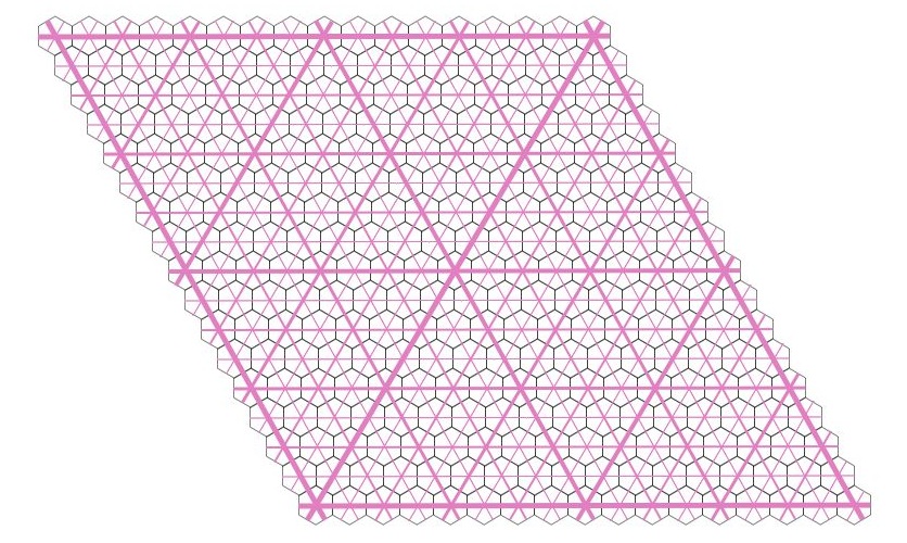
Figure 9. A partial triangulation of the plane overlaid on the basic lattice of hexagons which will make up the tiles. The levels of the triangles are indicated by increasing thickness. One can clearly see triangles of levels $0,1,2,3,4$ and one can also see how triangle edges of level $k$ ultimately become edges passing through the interior of triangles of level $k+1$. This will be used to make the shifting of edges later on.

The word ‘level’ occurs in a variety of senses in the paper. These are summarized in Table 1.

Table 1. Uses of the word ‘level’ $k$ and section number where it is defined. If there is no such $k$ the level is infinite.

of a triangle	§2 $k$ if the side length is $2^{k}$,
	where a side length $1=2^{0}$ is the length of $a_{1}$ and $a_{2}$
of orientation of $x\in P$	§2 $k$ at which $x$ stops switching between $S_{k}^{\uparrow}$ and $S_{k}^{\downarrow}$
of a $w$-line	§4 max. $k$ of centroids of level $k$ triangles on it
of a point of $Q$	§4 max. $k$ for which it is a vertex of a triangle of level $k$
of a triangle edge	§4 $k$ for which it is an edge of a level $k$ triangle
of an $a$-line	§4 max. $k$ for $k$-edges on this line

There are two types of generic assumptions that we need to consider.

Definition 4.1.

A triangulation (or the value of ${\bf q}$ associated with it) in which every w-line has a finite level is called generic-$w$. This means that for every w-line there is a finite bound on the levels of the centroids (points of $P\backslash Q$) that lie on that line. In this case for any ball of any radius anywhere in the plane, there is a level beyond which no w-lines of higher level cut through that ball. See Fig. 18 for an example that shows failure of the generic-w condition.

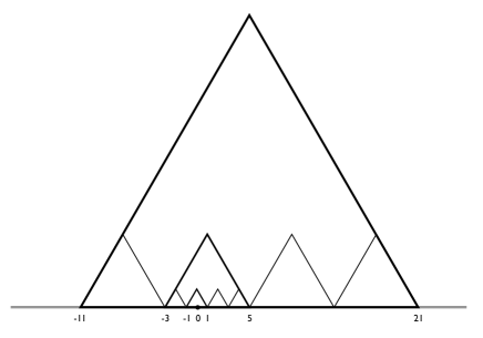
Figure 16. This shows a sketch of how a tiling with an infinite $a$-line (the horizontal line) can be constructed so that it is generic-w. Here ${\bf q}=za_{1}$, where $z$ is the $2$-adic integer $(1,1,5,5,21,21,85,85,\dots)$ (the $\mod 2,4,8,16,32,64,128,256\dots$ values). Some triangles of edge lengths $2,8,32$ are shown. There are triangles of arbitrary large side lengths on the horizontal line, but the triangulation does not admit a second infinite $a$-line and cannot admit an infinite $w$-line since ${\bf q}$ is of the wrong form.

A triangulation (or the value of ${\bf q}$ associated with it) is said to be generic-$a$ if every a-line has a finite level. This means for every a-line there is a finite bound on the levels of edges that lie in that line. In this case for any ball of any radius anywhere in the plane, there is a level beyond which no lines of the triangulation of higher level cut through that ball. See Fig. 16 and Fig. 18.

A tiling is said to be generic if it is both generic-w and generic-a. All other tilings (or elements ${\bf q}\in Q$) are called singular. One case of the failure of generic-w is discussed in Prop. 3.3 above. The only way for one of our generic conditions to fail is that there are a-lines or w-lines of infinite level. This situation is discussed in §6.

Every element of $Q$ has a hexagon around it and three lines passing through it in the directions $\pm a_{1},\pm a_{2},\pm(a_{1}+a_{2})$. These lines pass through pairs of opposite edges of the hexagon at right-angles to those edges. We shall call these lines short diameters. These short diameters arise out of the edges of the triangles of the triangulations that we have created. Each triangle edge is part of a line which is a union of edges, all of the same level. As we have pointed out, the line (and its edges) have level $k$ if they occur at level $k$ (and no higher). The original triangulation has level $0$. One should note that a line may occur as part of the edges of many levels of triangles, but under the assumption of generic-a there will be a highest level of triangles utilizing a given line, and it is this highest level that gives the line its level and determines the corresponding edges.

In looking at the construction of level $1$ triangles out of the original triangulation of level $0$ triangles, we note immediately that every point of $Q$ has at least one line of level $1$ through it (though by the time the triangularization is complete this line may have risen to higher level), see Fig. 6. The vertices of the level $1$ triangles have three lines of level $1$ through them, and the rest (the mid-points of the sides of the level $1$ triangles) have just one of level $1$ and the other two of level $0$. Thus at this stage of the construction each hexagon has either one short diameter from a level $1$ line or it has $3$ short diameters all of level $1$.

This is the point to remember: at each stage of determining the higher level triangles, we find that the hexagon around each element of $Q$ is of one of two kinds: it either has three short diameters of which two have equal level and the third a higher level, or three short diameters all of the same level $k$. The latter only occurs when the element of $Q$ is a vertex of a triangle of level $k$. Since we are in the generic-a case, there is no element of $Q$ which is a vertex of triangles of unbounded scales, and the second condition cannot hold indefinitely. Once an element of $Q$ is not a vertex at some level then it never becomes a vertex at any other higher level (all vertices of triangles at each level are formed from vertices of triangles at the previous level).

We conclude ultimately that in the generic-a cases every hexagon has three short diameters of which two are of one level and one of a higher level. See Fig. 9.

Lemma 4.2.

For ${\bf q}$ satisfying generic-a each hexagonal tile of $\mathcal{T}({\bf q})$ has three short diameters of which exactly one has the largest level and the other two equal but lesser levels.

We now describe edge shifting. Fix any $\epsilon$ with $0<\epsilon\leq 1/4$. This $\epsilon$ is going to be the distance by which lines are shifted. It is fixed throughout, but it exact value plays no role in the discussion. Take a tiling based on ${\bf q}$.

Now consider any edge that has level $k<\infty$ but does not occur as part of an edge of higher level. This edge occurs as an edge inside some triangle $T$ of level $k+1$, and this allows us to distinguish two sides of that edge. The side of the edge on which the centroid of $T$ lies is called the inner side of the edge, and the other side its outer side. This edge (but not the entire line) is shifted inwards (i.e. towards the centroid of $T$) by the distance $\epsilon$. Note that the shifting distance $\epsilon$ is independent of $k$. This shifted edge then becomes the black stripe on the hexagonal tiles through which this edge cuts, see Fig. 11. Fig. 10 shows how edge shifting works. At the end of shifting, each hexagon has on it a pattern made by the shifted triangle edges that looks like the one shown in Fig. 11.

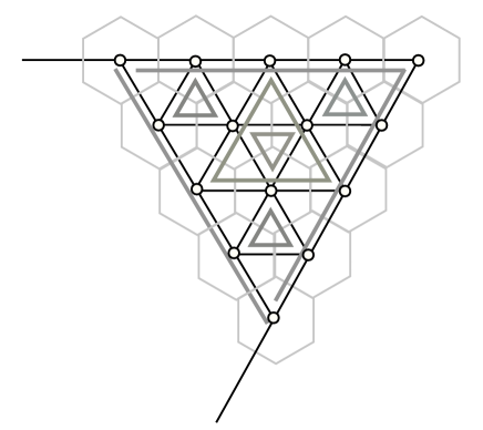
Figure 10. The figure shows how edge shifting is done. Part of a triangulation is shown in thin black lines. The shifted edges are shown in thicker gray lines. The extended black lines indicate that the largest (level $2$) triangle sits in the top right corner of a level $3$ triangle which is not shown in full. Note how the edges of the level $2$ triangle shift.

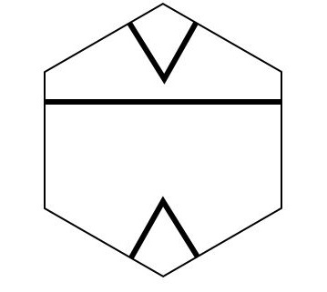
Figure 11. The basic hexagon with its markings arising from shrunken triangles.

In the case that ${\bf q}$ satisfies generic-a, the edges of every line of the triangulation are of bounded length. Thus every edge undergoes a shift by the prescription above. Thus,

Proposition 4.3.

If $\mathcal{T}({\bf q})$ satisfies the condition generic-a then there is a uniquely determined edge shifting on it. ∎

5. Color

So far we have constructed a triangulation from our choice of ${\bf q}$, and shown how edges can be shifted to produce the corresponding hexagonal tiling with the tiles suitably marked by black stripes. We wish now to show how the (long) diagonals of the hexagons are to be colored. This amounts to producing a color (red, blue, or red-blue) for each of the long diagonals of each hexagon of the tiling. The only requirement is that the overall coloring obey the rule ${\bf R2}$ that is used to make Taylor–Socolar tilings.

As we mentioned above, coloring is made independently of shifting in the sense that the two processes can be done in either order. In fact, in this argument we shall suppose that the stripes have not been shifted, so they still run through the centroids of the tiles.

We shall show that for $\bf{q}\in\overline{Q}$ in the generic case there is exactly one allowable coloring.

Assume that we have a generic tiling (this means both $a$ and $w$ generic). Now consider any hexagon of the tiling. We note from Lemma 4.2 that it has three short diameters, one of which is uniquely of highest level, and it is this last short diameter which determines (after shifting) the black stripe for this hexagon. We will refer to this short diameter as the stripe, even though in this discussion it has not been shifted. The other two colored (long) diameters are a red one which lies at $\pi/6$ clockwise of the stripe and a blue one which lies $\pi/6$ counterclockwise of the stripe. The red-blue diameter cuts the stripe at right-angles, but which way around it is (red-blue or blue-red) is not determined yet.

Consider Fig. 12 in which we see two complete level $1$ triangles overlaid on the basic level $0$ triangles. Tiles of the hexagonal tiling are shown on points of $Q$ with the hexagons at the vertices of the level $1$ triangles shown in green. These latter are points of $q_{1}+2Q$. At each point of $Q$ there are three edge lines running through it. But notice that at the midpoints of the sides of the level $1$ triangles (white hexagons), the edge belonging to the level $1$ triangle has higher level than the other two. This is the edge that will become the stripe for the hexagon at that point. This stripe forces the red and blue diameters for this hexagon.

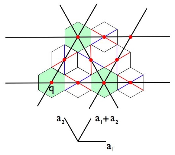
Figure 12. The figure shows some hexagonal tiles, each centered on a point of $Q$. The point $q$ is assumed to be in the coset $q_{1}+2Q$ and the gray hexagons are those in the picture whose centers are in this coset. The white hexagons are centered at points from all three of the remaining cosets of $Q$ relative to $2Q$. These are the midpoints of the edges of the level $1$ triangles. Notice in each, the red and blue diagonals clockwise and counterclockwise of the direction of the black stripes. At the bottom we see the three vectors $a_{1},a_{2},a_{1}+a_{2}$. The centers of the white hexagons are, reading left to right and bottom to top, $q_{1}+a_{1},q_{1}+3a_{1};q_{1}+a_{1}+a_{2},q_{1}+2a_{1}+a_{2},q_{1}+3a_{1}+a_{2};q_{1}+3a_{1}+2a_{2}$. The picture manifests the rule R2 and shows that elements of the same coset carry the same orientation of diameters. Note that from the rotational symmetry of the process and the fact that the hexagons centered on $q_{1}+a_{1}$ and $q_{1}+3a_{1}$ have identically aligned diagonals, we can infer that this property is retained across each of the cosets $q_{1}+a_{1}+2Q,q_{1}+a_{2}+2Q,q_{1}+a_{1}+a_{2}+2Q$.

The idea behind coloring is based on extrapolating this argument to w-lines passing through midpoints of higher level triangles. Consider Fig. 13. The point $u$ is the midpoint of an edge of a triangle $T^{\prime}$ of level $3$. Drawing the $w$-line $L$ towards the centroid $d$ of the top left corner triangle $T$ of level $2$ we see first of all that the edge of the level $3$ triangle through $u$ is the highest level edge through $u$ and hence the coloring along the $w$-line $L$ starts off red, as shown. Now the rule R2 forces the next part of the coloring to be blue and we come to the hexagon center $e$. This has three edges through it, but the one that our $w$-line crosses at right-angles has the highest level, and so will produce the stripe for the corresponding hexagon. The color must switch at the stripe, and so we see the next red segment as we come to $d$.

And so it goes, until we reach the point $v$. Here $L$ meets the midpoint of the edge of another level $3$ triangle. This edge produces the stripe for the hexagon at $v$, but it is not at right-angles to $L$, so there is no color change on $L$ at $v$. Since $v$ is the midpoint of this level $3$ triangle, the same argument that we used at $u$ shows that the coloring should start off blue, as indeed we have seen it does. At this point one can see by the glide reflection symmetry along $L$ that the entire line $L$ will ultimately be colored so as to fully respect the rule R2. For a full example where one can see the translational symmetry take over, the reader can fill in the coloring on the gray line through $y$.

One can see a similar $w$-line coloring of the $w$-line passing through $q$ and $c$. This time the point $q$ is the midpoint of an edge of a level $4$ triangle and $c$ is the centroid of one of the level $3$ corner triangles of this level $4$ triangle. The pair $r,c$ produces another example, with this time the first color out of $r$ being blue.

Finally, we show part of a potential line coloring starting at $s$ towards $t$. We say ‘potential’ because from the figure we do not know how the level $5$ triangles lie. If $s$ is a midpoint of an edge of a level $5$ triangle, then the indicated $w$-line is colored as shown. If $s$ is not a midpoint then this $w$-line is not yet colorable.

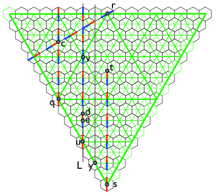
Figure 13. Coloring of lines. Colors are forced on $w$-lines as they pass through the midpoint of a triangle directed towards the centroid of one of its corner triangles.

We can thus continue in this way indefinitely. The important question is, does every tile get fully colored in the process? Using condition generic-w, the answer is yes. To see this note that each element of $p$ of $P\backslash Q$ has three coloring lines through it. It will suffice to prove that the process described above will color these three coloring lines.

Now assuming the condition generic-w we know that $p$ has an orientation. This means that it is the centroid of some triangle $T$ of level $k$ in the triangulation, and it is not the centroid of any higher level triangle. The triangle $T$ then sits as one of the corner triangles in a triangle $T^{\prime}$ of level $k+1$. Up to orientation, the situation is that shown in Fig. 14. The colors of the two hexagons shown are then determined because the edges of $T^{\prime}$ produces stripes on them. Thus the two corresponding coloring lines that pass through $p$ are indeed colored. Thus the colorings of these two coloring lines through $p$, the ones that pass through the mid-points of two sides of $T^{\prime}$ are forced.

What about the third line $l$ through $p$ (shown as the dotted line in Fig. 14)? We wish to see this as a w-line through a midpoint of an edge, just as we saw the other two lines. We look at the centroid $p^{\prime}$ of $T^{\prime}$, since the coloring line $l$, which is through $v$ and $p$, is the same as the line through $v$ and $p^{\prime}$ and the centroid $p^{\prime}$ is of higher level than $p$ and also has an orientation. We can repeat the process we just went through with $p$ with $p^{\prime}$ instead, to get a new triangle $T^{\prime\prime}$ of which $p^{\prime}$ is the centroid, and a triangle $T^{\prime\prime\prime}$ in which $T^{\prime\prime}$ sits as one of its corners ($p^{\prime}$ is the centroid of $T^{\prime}$ but it may be the centroid of higher level triangles as well).

If this still fails to pick up the line $l$ then it must be that $l$ still passes through a vertex of $T^{\prime\prime\prime}$ (as opposed to through the midpoint of one of its edges) and the line $l$ passes through the centroid $p^{\prime\prime\prime}$ of $T^{\prime\prime\prime}$. However, $p^{\prime\prime\prime}$ is of higher level still than that of $p^{\prime}$. The upshot of this is that if we never reach a forced coloring of $l$ (so that it remains forever uncolored in our coloring process) then we have on the line $l$ centroids of triangles of unbounded levels. This violates condition generic-w. Thus in the generic situation the coloring does reach every coloring line and the coloring is complete in the limit.

This completes the argument that there is one and only one coloring for each generic triangularization.

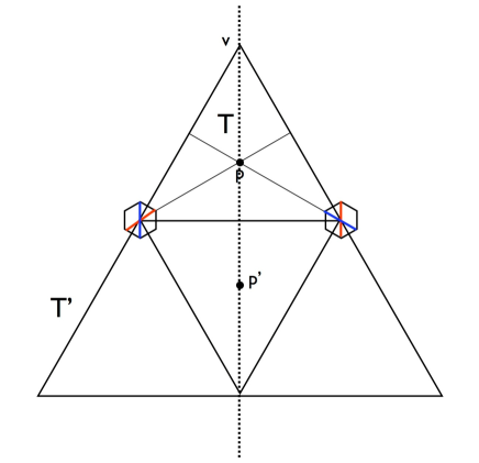
Figure 14. The figure shows how the centroid of the triangle $T$, which is in the top corner of the main triangle, is on two coloring lines. The third coloring line through $p$ is the dotted line through $v$. This passes through the centroid $p^{\prime}$ of $T^{\prime}$.

If one is presented with a triangularization and wishes to put in the colors, then one sees that the coloring becomes known in stages, looking at the triangles (equivalently cosets) of ever increasing levels. Figure 15 shows the amount of color information that can be gleaned at level $k=2$.

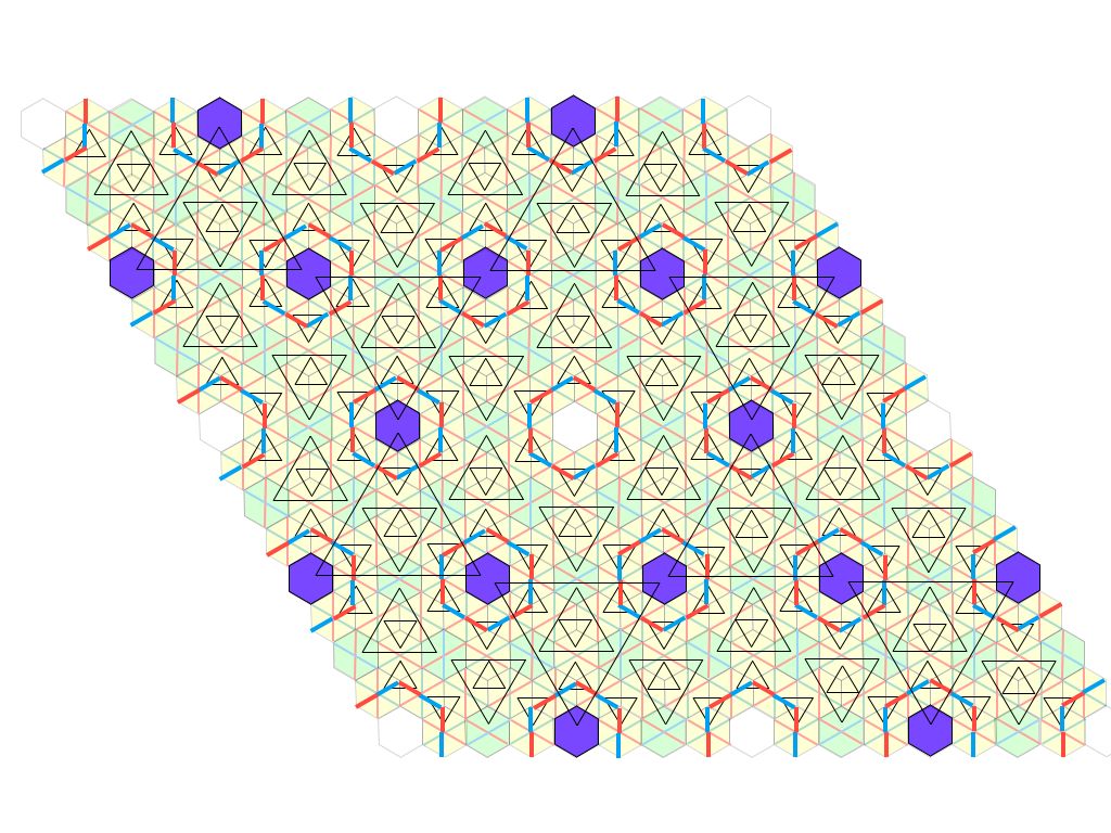
Figure 15. This figure shows how the coloring appears if one determines the coloring by the information in increasing coset levels. This figure corresponds to the process at $k=2$. The triangle vertices and their corresponding hexagons are indicated at levels $0,1,2$ and the corresponding partial coloring is noted.

Proposition 5.1.

Any generic tiling is uniquely colorable. ∎

We note that in the generic situation, the shifting and coloring are determined locally. That is, if one wishes to create the marked tiles for a finite patch of a generic tiling, one need only examine the tiling in a finite neighbourhood of that patch. That is because the shifting and coloring depend only on knowing levels of lines, and what the levels of various points on them are. Because of the generic conditions, these levels are all bounded in any finite patch and one needs only to look a finite distance out from the patch in order to pick up all the appropriate centroids and triangle edges to decide on the coloring and shifting within the patch. Of course the radii of the patches are not uniformly bounded across the entire tiling.

Here we offer a different proof of a result that appears in [19]:

Proposition 5.2.

In any generic tiling and at any point $p$ which is a hexagon vertex, the colors of the three concurrent diagonals of the three hexagons that surround $p$ are not all the same (where they meet at $p$).

Proof: The point $p$ is the centroid of come corner triangle of one of the triangles of the triangulation. Fig. 14 shows how the coloring is forced along two of the medians of the corner triangle and that they force opposite colorings at $p$. See also Fig. 27. ∎

5.1. Completeness

We have now shown how to work from a triangularization to a tiling satisfying the matching rules R1,R2. Does this procedure produce all possible tilings satisfying these rules? The answer is yes, and this is already implicit in [19]. We refer the reader to the paper for details, but the point is that in creating a tiling following the rules a triangle pattern emerges from the stripes of the hexagons. This triangularization can be viewed as the edge-shifting of a triangulation $\mathcal{T}$ conforming to our edge shifting rule. Thus we know that working with all triangulations, as we do, we are bound to be able to produce the same shrunken triangle pattern as appears in $T$.

In the generic cases, the coloring that we impose on this triangulation is precisely that forced by R2. When we discuss the non-generic cases in §6.2, we shall see that for non-generic triangulations there are actually choices for the colorings of some lines, but these choices exhaust the possibilities allowed by the rule R2. Thus the tiling $T$ must be among those that we construct from $\mathcal{T}$ and so we see that our procedure does create all possible tilings conforming to the matching rules.

When we determine the structure of the hull in §6.4 we shall also see that it is comprised of a minimal hull and two highly exceptional countable families of tilings. The former contains triangulations of all types and, as the terminology indicates, the orbit closure of any one of its tilings contains all the others in the minimal hull, so in a sense if you have one then you have them all. (The two exceptional families of tilings appear in the rule based development of the tilings, but do not appear in the inflation rule description.)

6. The Hull

6.1. Introducing the hull

Let $X_{Q}$ denote the set of all Taylor–Socolar hexagonal tilings whose hexagons are centered on the points of $Q$ and whose vertices are the points of $P\backslash Q$. The group $Q$ (with the discrete topology) acts on $X_{Q}$ by translations. We let $X$ be the set of all translations by $\mathbb{R}\hskip 0.5pt^{2}$ of the elements of $X_{Q}$. We call $X_{Q}$ and $X$ the hulls of the Taylor–Socolar tiling system. We give $X_{Q}$ and $X$ the usual local topologies - two tilings are close if they agree on a large ball around the origin allowing small shifts. In the case of $X_{Q}$ one can do away with ‘the small shifts’ part. See [13] for the topology.

In fact it is easy to see that, although we have produced it out of $X_{Q}$, $X$ is just the standard hull that one would expect from the set of all Taylor–Socolar tilings when they have not been anchored onto the points of $Q$. Thus $X$ is compact, and since $X_{Q}$ is a closed subset of it, it too is compact.

The translation actions of $Q$ on $X_{Q}$ and $\mathbb{R}\hskip 0.5pt^{2}$ on $X$ are continuous. We note that the hulls $X_{Q}$ and $X$ are invariant under six-fold rotation and under complete interchange of the two tile types. Our task is to provide some understanding of $X_{Q}$ and $X$. Here we shall stick primarily to $X_{Q}$ since the corresponding results for $X$ are easily inferred. We let $X_{Q}^{gen}$ denote the set of all the generic tilings in $X_{Q}$.

Each element $\Lambda\in X_{Q}$ produces a triangularization of the plane, and the triangularizations are parameterized precisely by elements in $\overline{Q}$. In particular there is an element ${\bf q}(\Lambda)\in\overline{Q}$ corresponding to $\Lambda$, and we have a surjective mapping

(3) $$\xi:X_{Q} \longrightarrow \overline{Q}$$

$$\Lambda \mapsto {\bf q}(\Lambda)\,.$$

Proposition 6.1.

The mapping $\xi$ is continuous (with respect to the local topology on $X_{Q}$ and the $Q$-adic topology on $\overline{Q}$). Furthermore $\xi$ is $1-1$ on $X_{Q}^{gen}$.

Proof: Any ${\bf q}\in\overline{Q}$ is determined by its congruence classes modulo $2\overline{Q},4\overline{Q},\dots$, which are represented equally well by the congruence classes of $Q$ modulo $2Q,4Q,\dots$. These congruence classes are the sets of vertices of the triangles of increasing sizes, starting with those of level $1$. Now any patch of tiles containing a ball $B_{R}$, $R>2$, will determine part of the triangulation with triangles of all levels $1,2,\dots n$ for some $n=n(R)$, and we have $n(R)\to\infty$ as $R\to\infty$. The larger the patch the more congruence classes we know, and this is the continuity statement.

In the case of a generic tiling $\Lambda$, ${\bf q}(\Lambda)$ already determines the entire markings of the tiles and hence determines $\Lambda$. Thus $\xi$ is $1-1$ on $X_{Q}^{gen}$.∎

Below we shall see that with respect to the Haar measure on $\overline{Q}$ the set of singular (i.e. non-generic) ${\bf q}$ is of measure $0$. A consequence of this is [5], Thm. 6:

Corollary 6.2.

$X_{Q}$ is uniquely ergodic and the elements of $X_{Q}^{gen}$ are regular model sets. ∎

We shall make the model sets rather explicit in §7.

6.2. Exceptional cases

We now consider what happens in the case of non-generic tilings. To be non-generic a tiling must violate either generic-a or generic-w. We consider these two situations in turn.

6.2.1. Violation of generic-a

In the case of violation of generic-a, there is an a-line of infinite level (that is, it does not have a level as we have defined it). Let $\overline{\mathbb{Z}_{2}}$ be the $Q$-adic completion of $\mathbb{Z}$.

Proposition 6.3.

A tiling $\Lambda$, where $\xi(\Lambda)={\bf q}$, has an a-line of infinite level if and only if   ${\bf q}\in x+\overline{\mathbb{Z}_{2}}a$ for some $a\in\{a_{1},a_{2},a_{1}+a_{2}\}$ and some $x\in Q$. Furthermore when this happens the points of $Q$ lying on the infinite-level-line are those of the set $x+{\mathbb{Z}}a$.

Proof: All lines of the triangulation are in the directions $\pm a_{1},\pm a_{2},\pm(a_{1}+a_{2})$ and all lines of the triangulation contain edges of all levels from $0$ up to the level of the line itself. Thus the points of $Q$ on any line $l$ of the triangulation are always a set of the form $x+\mathbb{Z}a$ where $a\in\{a_{1},a_{2},a_{1}+a_{2}\}$ and $x\in Q\cap l$.

Suppose that we have a line $l$ of infinite level and its intersection with $Q$ is contained in $x+\mathbb{Z}a$. The line $l$ has elements $y_{1},y_{2},\dots$ where $y_{k}$ is a vertex of a triangle of level $k$. This means that $y_{1}\in q_{1}+2Q,y_{2}\in q_{1}+q_{2}+4Q,\dots$. We conclude that $\{y_{k}\}\to{\bf q}$. Furthermore $y_{k+1}-y_{k}\in 2^{k}Q\cap\mathbb{Z}a=2^{k}\mathbb{Z}a$. This is true for all $k\geq 0$ if we define $y_{0}=x$. Writing $y_{k+1}-y_{k}=2^{k}u_{k}a$ with $u_{k}\in\mathbb{Z}$ and ${\bf u}=(0,u_{1},\dots,\sum_{j=1}^{k}u_{j}2^{j},\dots)$, we have

$$y_{k+1}=x+\left(\sum_{j=1}^{k}u_{j}2^{j}\right)a\ \rightarrow\ x+{\bf u}a$$

where ${\bf u}\in\overline{\mathbb{Z}_{2}}$. Thus ${\bf q}=x+{\bf u}a$. This proves the only if part of the Lemma.

Going in the reverse direction, if ${\bf q}=x+{\bf u}a$ then this is a prescription for a line of points in $Q$ that have vertices of all levels. Then the line is of infinite level. ∎

Proposition 6.4.

If a tiling $\Lambda\in X_{Q}$ has an infinite a-line then it is in $X_{Q}\backslash X_{Q}^{gen}$ and has either precisely one infinite a-line or three infinite a-lines which are concurrent. The latter case occurs if and only if ${\bf q}\in Q$, where ${\bf q}=\xi(\Lambda)$.

Proof: Let $\Lambda\in X_{Q}$ have an infinite a-line $l$. We already know that $\Lambda\in X_{Q}\backslash X_{Q}^{gen}$ and ${\bf q}=x+{\bf u}a$ for some $x\in Q$, ${\bf u}\in\overline{\mathbb{Z}_{2}}$, and some $a\in\{a_{1},a_{2},a_{1}+a_{2}\}$ from Lemma 6.3. If it has a second (different) infinite line $l^{\prime}$ then similarly ${\bf q}=y+{\bf v}b$ where $y\in Q$, ${\bf v}\in\overline{\mathbb{Z}_{2}}$, and $b\in\{a_{1},a_{2},a_{1}+a_{2}\}$. Certainly $a\neq b$ for otherwise the two lines are parallel and this leads to overlapping triangles of arbitrarily large size, which cannot happen. But we have $y-x\in Q\cap(\overline{\mathbb{Z}_{2}}a+\overline{\mathbb{Z}_{2}}b)=\mathbb{Z}a+\mathbb{Z}b$. Since $a,b$ are linearly independent over $\overline{\mathbb{Z}_{2}}$ and $y-x={\bf u}a-{\bf v}b$ we see that ${\bf u}$ and ${\bf v}$ are actually in $\mathbb{Z}$. Then ${\bf q}\in Q$. We will indicate this by writing $q$ for ${\bf q}$.

In this case, since $q\equiv q_{1}+\cdots+q_{k}\mod 2^{k}Q$ we find that $q$ is a vertex of a level $k$ triangle, for all $k$. Since this is true for all $k$, $q$ is a point through which infinite level lines in all three directions $\{a_{1},a_{2},a_{1}+a_{2}\}$ pass. Thus the existence of two infinite lines implies the existence of three concurrent lines.

In the other direction, if ${\bf q}\in Q$ then as we have just seen there will be three concurrent infinite lines passing through it. ∎

The case of a tiling with three concurrent infinite a-lines in Proposition 6.4 is called a central hexagon tiling (CHT tiling) in [19]. We also refer to them as iCa-L tilings. Edge shifting is not defined along these three lines, and we shall see that we have the freedom to shift them arbitrarily to produce legal tilings. The tilings in which there is one infinite a-line are designated as ia-L tilings.

6.2.2. Violation of generic-w

The case of violation of generic-w is somewhat similar, though it takes more care. One aspect of this is to avoid problems of $3$-torsion in $\overline{P}$, which we shall do by staying inside $\overline{Q}$ where this problem does not occur. Thus in the discussion below the quantity $3w$, where $w\in\{w_{1},w_{2},w_{2}-w_{1}\}$, is of course in $Q$, but when we see it with coefficients from $\overline{\mathbb{Z}_{2}}$ we shall understand it as being in $\overline{Q}$ (as opposed to being in $\overline{P}$). Another problem is that the violation of generic-w is not totally disjoint from the violation of generic-a, as we shall see.

Proposition 6.5.

$\Lambda({\bf q})$ has a w-line of infinite level if and only if   ${\bf q}\in x+\overline{\mathbb{Z}_{2}}\,3w$ for some $w\in\{w_{1},w_{2},w_{2}-w_{1}\}$ and some $x\in Q$. Furthermore when this happens the points of $Q$ lying on the infinite-level-line are those of the set $x+{\mathbb{Z}}\,3w$.

Proof: All w-lines deriving from the triangulation are necessarily in the directions $w\in\{\pm w_{1},\pm w_{2},\pm(w_{2}-w_{1})\}$. Of course $3w\in Q$, and $mw\in Q$ iff $3|m$. It really makes no difference which of the six choices $w$ is, but for convenience in presentation we shall take herewith $w=w_{2}$ so that $3w=a_{1}+2a_{2}$. This is in the vertical direction in the plane.

All w-lines contain centroids of levels up to the level of the line itself. Furthermore if a w-line contains a centroid of level $k$ then it also contains one of the vertices of the corresponding triangle and so also at least one point of $Q$ of level $k$. It follows that for any w-line $l$ in the direction $w$ there is an $x\in Q$ so that the set of points of $Q$ on $l$ is the set $x+\mathbb{Z}\,3w=x+\mathbb{Z}(a_{1}+2a_{2})$.

Suppose that we have a w-line $l$ of infinite level and its intersection with $Q$ is $x+\mathbb{Z}(a_{1}+2a_{2})$. Then the line $l$ has elements $y_{1},y_{2},\dots$ where $y_{k}$ is a vertex of a triangle of level $k$. This means that $y_{1}\in q_{1}+2Q,y_{2}\in q_{1}+q_{2}+4Q,\dots$. We conclude that $\{y_{k}\}\to{\bf q}$. Furthermore $y_{k+1}-y_{k}\in 2^{k}Q\cap\mathbb{Z}(a_{1}+2a_{2})$. This is true for all $k\geq 0$ if we define $y_{0}=x$. Writing $y_{k+1}-y_{k}=2^{k}u_{k}(a_{1}+2a_{2})$ with $u_{k}\in\mathbb{Z}$ and ${\bf u}=(0,u_{1},\dots,\sum_{j=1}^{k}u_{j},\dots)\in\overline{\mathbb{Z}_{2}}$, we have

$$y_{k+1}=x+\left(\sum_{j=0}^{k}u_{j}2^{j}\right)\,(a_{1}+2a_{2})\rightarrow x+{\bf u}\,(a_{1}+2a_{2}).$$

Thus ${\bf q}=x+{\bf u}\,(a_{1}+2a_{2})$. This proves the only if part of the Lemma.

Going in the reverse direction, if ${\bf q}=x+{\bf u}\,(a_{1}+2a_{2})$ then this is a prescription for a line of points in $Q$ that have vertices of all levels. The corresponding w-line has centroids of unbounded levels, so the line is a w-line of infinite level. ∎

Proposition 6.6.

If a tiling $\Lambda\in X_{Q}$ has an infinite w-line then $\Lambda\in X_{Q}\backslash X_{Q}^{gen}$ and it has either precisely one infinite w-line or three infinite w-lines which are concurrent. The latter case occurs if and only if the point of concurrency is either a point of infinite level (discussed in Prop. 6.4) or a non-orientable point (discussed in Prop. 3.3).

Proof: Let $\Lambda\in X_{Q}$ have an infinite w-line $l$. We again take this to be in the direction of $w_{2}$. Then ${\bf q}:=\xi(\Lambda)=x+{\bf u}\,(a_{1}+2a_{2})$ for some $x\in Q$, ${\bf u}\in\overline{\mathbb{Z}_{2}}$.

Suppose that it has a second (different) infinite line $l^{\prime}$. Then similarly ${\bf q}=y+{\bf v}\,3w^{\prime}$ where $y\in Q$, ${\bf v}\in\overline{\mathbb{Z}_{2}}$, and $3w^{\prime}\in\{2a_{1}+a_{2},a_{1}+2a_{2},a_{2}-a_{1}\}$. As above, we note that $w\neq w^{\prime}$ because if $w=w^{\prime}$, the two lines are parallel and each of the two lines contains vertices of arbitrarily large levels. But the parallel lines through vertices and centroids of level $k$ are spaced at a distance of $2^{k-1}$ apart. Thus no two distinct parallel w-lines can both carry centroids of arbitrary level.

Again, for concreteness we shall take a specific choice for $w^{\prime}$, namely $w^{\prime}=w_{1}=2a_{1}+a_{2}$. Other choices lead to similar results.

There are two scenarios. Either the two lines $l,l^{\prime}$ meet at a point of $Q$ or not. Suppose that they meet in a point of $Q$. Then we can choose $x=y$ and obtain

$$x+{\bf u}\,(a_{1}+2a_{2})={\bf q}=x+{\bf v}\,(2a_{1}+a_{2})\,.$$

Since $a_{1}$ and $a_{2}$ are independent in $\overline{Q}$ over $\overline{\mathbb{Z}_{2}}$ we obtain ${\bf u}=2{\bf v}$ and ${2\bf u}={\bf v}$. The only solution to this in $\overline{\mathbb{Z}_{2}}$ is ${\bf u}={\bf v}=0$. Thus ${\bf q}=x\in Q$. This puts us in the situation of Prop. 6.4, the point of intersection of the two lines is actually a vertex of infinite level, and this is a CHT tiling.

The alternative is that $l,l^{\prime}$ meet at a point $p$ of $P\backslash Q$. In this case we go back to the discussion of coloring given in §5. The point $p$ is a centroid and it either has infinite level, in which case it has no orientation and we go to Prop. 3.3, or it has a finite level in which two of the three w-lines through it have forced color and finite level which is a contradiction. This proves the result. ∎

Infinite level a-lines occur if and only if ${\bf q}\in x+\overline{\mathbb{Z}_{2}}a$ and infinite level w-lines occur if and only if ${\bf q}\in x+\overline{\mathbb{Z}_{2}}w$, with $a,w$ being in the basic $a$ and $w$ directions respectively. Three concurrent a-lines occur if and only ifs ${\bf q}\in Q$, whereupon the condition for three concurrent w-lines also is true. These are the CHT tilings.

Table 2. Summary of infinite level $a$-lines and $w$-lines.

type	single	three concurrent
infinite $a$-line	${\bf q}\in Q+\overline{\mathbb{Z}_{2}}a$	${\bf q}\in Q$  CHT
infinite $w$-line	${\bf q}\in Q+\overline{\mathbb{Z}_{2}}w$	${\bf q}\in Q$  CHT
		${\bf q}\in-{\bf s_{2}}-2{\bf s_{1}}+Q$  or   ${\bf q}\in-{\bf s_{1}}-2{\bf s_{2}}+Q$

Since the singular elements of $\overline{Q}$ lie on a countable union of lines, it is clear that their total measure is $0$.

Lemma 6.7.

The set of singular ${\bf q}\in Q$ has Haar measure $0$.

Lemma 6.8.

If a triangularization ${\mathcal{T}}({\bf q})$ has both an infinite level $a$-line and an infinite level $w$-line then their point of intersection is a point of concurrence of three infinite level w-lines and three infinite level a-lines, and the tiling is a CHT tiling.

Proof: By Prop. 6.3 and Prop. 6.5,

$${\bf q}\in x_{1}+\overline{\mathbb{Z}_{2}}a\quad\mbox{and}\quad{\bf q}\in x_{2}+\overline{\mathbb{Z}_{2}}3w$$

for some $x_{1},x_{2}\in Q$ and $a\in\{a_{1},a_{2},a_{1}+a_{2}\}$, $w\in\{w_{1},w_{2},w_{2}-w_{1}\}$. Putting these together,

$${\bf q}=x_{1}+{\bf z_{1}}a=x_{2}+{\bf z_{2}}3w$$

for some ${\bf z_{1},z_{2}}\in\overline{\mathbb{Z}_{2}}$. However $a$ and $3w$ are independent elements of $Q$ (over $\mathbb{Z}$), and hence are also independent over $\overline{\mathbb{Z}_{2}}$. Since $x_{2}-x_{1}\in Q$, this forces ${\bf z_{1},z_{2}}\in\mathbb{Z}$. Thus ${\bf q}\in Q$, which is the condition for simultaneous concurrency of three a-lines and three w-lines (Prop. 6.4). ∎

6.3. Coloring for the iCw-L tilings

According to Prop. 3.3 we have a point of no orientation precisely when ${\bf q}\in-{\bf s_{2}}-2{\bf s_{1}}+Q$ or ${\bf q}\in-{\bf s_{1}}-2{\bf s_{2}}+Q$. In these cases, by Prop. 6.6, we have three concurrent w-lines and their intersection is a point of no orientation. This point of intersection is $x={\bf q}+w_{1}+{\bf s_{2}}+2{\bf s_{1}}$ or $x={\bf q}+w_{2}+{\bf s_{1}}+2{\bf s_{2}}$. The former can be anywhere in $w_{1}+Q$ and the latter anywhere in $w_{2}+Q$. The triangulation can be described as a set of nested triangles of levels $0,1,2,3,\dots$ (and all the lesser level triangles that occur within them) all of which have the centroid $x$. The level $k=0$ triangle is an up triangle in the $w_{1}$ case and a down triangle in the $w_{2}$ case. The infinite $l$-lines are in the directions $w_{1},w_{2},w_{2}-w_{1}$ through $x$ and these three lines have no forced colorings.

We call these tilings the iCw-L tilings (infinite concurrent w-line tilings). We also refer to the underlying triangulations with the same terminology. See Figure 18.

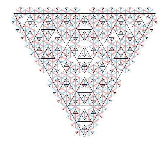
Figure 18. The iCw-L tilings. The triangulation is generic-a but not generic-w. Of course the partial tiling shown is perfectly consistent with generic tilings – in fact all Taylor–Socolar tilings contain this type of patch of tiles. However, if the pattern established in the picture is maintained at all scales, then indeed the result is a not a generic tiling since it fails generic-$w$.

The symmetry belongs to the triangulation, not necessarily to the tilings themselves. The colorings of the three exceptional lines of an iCw-L tiling can be made in an arbitrary way without violating the tiling conditions R1, R2  [19]. Of the $8$ possible colorings the two truly symmetric ones (the ones that give an overall $3$-fold rotational symmetry – including color symmetry – to the actual tiling) are exceptional in the sense that no other tilings in the Taylor–Socolar system have a point $p\in P\backslash Q$ (i.e a tile vertex) with the property that the three hexagon diagonals emanating from it are all of the same color (see Prop. 5.2). These exceptional symmetric iCw-L tilings are called SiCw-L tilings. In [19] these tilings are described as having a ‘defect’ at this point, and indeed they are not LI to any other tilings except other SiCw-L tilings.

Thus there are $2$ exceptional colorings for any iCw-L triangulation. In the other $6$ colorings there are at each hexagon vertex two diameters of the same color and one of the opposite color, and we shall soon prove that they all occur in $X_{Q}$.

Tilings for which there is just one infinite w-line in the triangulation are called iw-L tilings.

6.4. The structure of the hull

In this subsection we describe the hull $X_{Q}$ in more detail. We note that the only symmetries of $X_{Q}$ which we discuss are translational symmetries (not rotational). These translational symmetries are the elements of $Q$. Of course none of the elements of $X_{Q}$ has any non-trivial translational symmetry; it is only the hull itself that has them. When we discuss LI classes below we mean local indistinguishability classes under translational symmetry.

Theorem 6.9.

$X_{Q}$ consists of three LI classes, $X_{Q}^{b}$, $X_{Q}^{r}$, and $X_{Q}^{\dagger}$. Of these $X_{Q}^{b}$ is the countable set of SiCw-L tilings with three blue-red (blue first) diameters emanating from some hexagon vertex $q$, which form a single $Q$-orbit in $X_{Q}$, and $X_{Q}^{r}$ is the companion orbit with red-blue diameters. Both of these orbits are dense in $X_{Q}$.

$X_{Q}^{\dagger}$ is the orbit closure of $X_{Q}^{gen}$ and contains all other tilings, including all the iCw-L tilings that are not color symmetric. Restricted to the minimal hull $X_{Q}^{\dagger}$, the mapping $\xi$ defined in (3) is:

• $1:1$ on $X_{Q}^{gen}$;

• $6:1$ at iCw-L points except SiCw-L points

• $12:1$ at CHT points;

• $2:1$ at all other non-generic points.

Remark 6.10.

The images of $\xi$ of the set of singular points (non-generic points) is dense in $\overline{Q}$. For instance, the triangulations with three concurrent a-lines are parameterized by $Q$ which is a dense subset of $\overline{Q}$, and these tilings produce the CHT tilings (or iCa-L tilings) described above. Both $X_{Q}^{gen}$ and $X_{Q}^{\dagger}$ are of full measure in $X_{Q}$.

Proof: First, we consider generic tilings. Let $\Lambda$, where $\xi(\Lambda)={\bf q}$, be any generic tiling and let $B_{R}$ be the ball of radius $R$ centered on $0$. Let $\mathcal{T}(\Lambda)$ be the triangulation determined by $\Lambda$ (with edges not displaced) and let $\mathcal{T}_{R}(\Lambda)$ be the part of the triangulation that is determined by $B_{R}$.

Because we are in a generic situation, to know how to shift an edge of level $k$ we need only that edge to appear as an inner edge of a triangle of level $k+1$. To determine the coloring of a w-line we need to know its level (which is finite). So to know all this information for $\mathcal{T}_{R}$ we need only choose $r$ large enough so that $B_{r}$ contains all the appropriate triangles.

Now if generic $\Lambda^{\prime}$, where $\xi({\Lambda^{\prime}})={\bf q^{\prime}}$ produces the same pattern of triangles in $B_{r}$ then it is indistinguishable from $\Lambda$ in $B_{R}$. In particular if ${\bf q^{\prime}}$ satisfies ${\bf q^{\prime}}-{\bf q}\in 2^{k}Q$ for large enough $k$ then $\Lambda$ and $\Lambda^{\prime}$ must agree (as tilings) on $B_{R}$. This proves that convergence of ${\bf q^{\prime}}$ to ${\bf q}$ produces corresponding convergence in $X_{Q}$.

With this it is easy to see that any two generic elements of $X$ are LI. Let $\xi(\Lambda)={\bf q}$ and $\xi(\Lambda^{\prime})={\bf q^{\prime}}$ be generic. Let ${\bf q}$ correspond to $q_{1},q_{2},\dots$ and ${\bf q^{\prime}}$ correspond to $q^{\prime}_{1},q^{\prime}_{2},\dots$. Then we can construct the tiling sequence $q^{\prime}_{1}-q_{1}+\Lambda,q^{\prime}_{1}+q^{\prime}_{2}-(q_{1}+q_{2})+\Lambda,\dots$ and it converges to $\Lambda^{\prime}$.

This same argument can be used to show that the orbit closure of any tiling contains all of $X_{Q}^{gen}$. Let $\Lambda$ be any tiling with ${\bf q}=\xi(\Lambda)$ and $\Lambda^{\prime}$ be a generic tiling with ${\bf q^{\prime}}=\xi(\Lambda^{\prime})$. Then one simply forms a sequence of translates of $\Lambda$ that change ${\bf q}$ into ${\bf q}^{\prime}$. The convergence of the triangulation on increasing sized patches forces convergence of the color and we see $\Lambda^{\prime}$ in the orbit closure of $\Lambda$.

Second, we consider the iCw-L cases, where $x:={\bf q}+w_{2}+{\bf s_{1}}+2{\bf s_{2}}\in w_{2}+Q$ or $x:={\bf q}+w_{1}+{\bf s_{2}}+2{\bf s_{1}}\in w_{1}+Q$. In these cases $x$ is a non-orientable point and there exists a nested sequence of triangles of all levels centered on $x$. This sequence begins either with an up triangle of level $0$ or a down triangle of level $0$. In either case everything about the triangulation is known and the entire tiling is determined except for the coloring of the three w-lines through $x$. In fact all of the $8$ potential colorings of these three lines are realizable as tilings, as we shall soon see.

Of these iCw-L triangulations we have the SiCw-L tilings in which the colors of the diagonals of the three hexagons of which $x$ is a vertex start off the same – all red or all blue. This arrangement at a hexagon vertex never arises in a generic tilings, and it is for this reason that these tilings produce different LI classes than the one that the generic tilings lie in: one ‘red’ LI class and one ‘blue’ LI class. As pointed out in [19] these SiCw-L tilings have the amazing property that they are completely determined once the three hexagons around $x$ have been decided. The form of the points $x$ with no orientation shows that there are just two $Q$ orbits of them, one for each of the two non-trivial cosets of $Q$ in $P$.

What about the other $6$ color arrangements around such a point $x$? Here we can argue that they all exist in the following way. Since in any triangulation there are tile centroids of any desired level $k$, we can start with any generic $\Lambda$ and form a sequence of translates of it that have centroids of ever increasing level at $0$. The sequence has at least one limit point and this is an iCw-L tiling. Since each element of the sequence has a unique coloring and coloring in generic tiles is locally determined by local conditions, there must be a subsequence of these tilings that converges to one of some particular coloring. This must produce a coloring of diameters with two diameters of one color and one of the other color since we are using only generic tilings in the sequence. Now the rotational three-fold symmetry and the color symmetry of $X_{Q}$ shows that all $6$ possibilities for the coloring will exist. This also shows that all these tilings are in the orbit closure of $X_{Q}^{gen}$.

Third, the CHT/iCa-L triangulations have the form $\mathcal{T}(q)$ where $q\in Q$. They have three concurrent a-lines and three concurrent w-lines at $q$ and leave the central tile completely undetermined. This tile can be placed in anyway we wish, and this fixes the entire tiling. There are a total of $12$ ways to place this missing tile ($6$ for each parity), whence $\xi$ is $12:1$ over $q$.

Finally, apart from the iCw-L and CHT/iCa-L tilings, the remaining singular values of q correspond to the ia-L and iw-L triangulations where there is either a single infinite level $a$-line or a single infinite level $w$-line, §6.3. Fortunately these two things cannot happen at the same time, see Lemma 6.8. That means that there is only one line open to question and there is only one line on which either the shift or color is not determined. In the ia-L case there is an $a$-line for which edge shifting is un-defined and we wish to show that all the two potentially available shifts lead to valid tilings. Likewise in the iw-L case there is a $w$-line to which no color can be assigned, and we wish to prove that both coloring options are viable.

Suppose one starts with a CHT tiling $\Lambda$ centered at $0$. If one forms a sequence $\{q_{1}+\cdots+q_{k}+\Lambda\}$ of CHT tilings and if $\{q_{1}+\cdots+q_{k}\}$ converges to a point of on the line $\overline{\mathbb{Z}_{2}}a_{1}$ that is not in $Q$ then the point of CHT concurrence has vanished and one is left only with the $x$-axis as an single infinite level a-line, and it will have the shifting induced by the original shifting along the $x$-axis in $\Lambda$ (which can be either of the two potential possibilities). Of course one can do this in any of the $a$ directions. A similar type of procedure works to produce all of the iw-L tilings. This concludes the proof of the theorem. ∎

7. Tilings as model sets

In this section we consider Taylor–Socolar tilings, and in particular the parity sets of such tilings, from the point of view of model sets. There are a number of advantages to establishing that point sets are model sets since there is a very extensive theory for them, including fundamental theorems regarding their intricate relationship to their autocorrelation measures and their pure point diffractiveness [18, 6, 5]. In fact there are various ways in which one can establish that the vertices or the tile centres of a Taylor–Socolar tiling always form a model set. We have already pointed this out in Cor. 6.2. However, the set-up that we have created makes it easy to see the model set construction rather explicitly, and that is the purpose of this section.

The basic pre-requisite for the cut and project formalism is a cut and project scheme. Most often, especially in mathematical physics, the cut and project schemes have real spaces (i.e. spaces of the form $\mathbb{R}\hskip 0.5pt^{n}$) as embedding spaces and internal spaces. But the theory of model sets is really part of the theory of locally compact Abelian groups [14]. In the case of limit-periodic sets, some sort of “adic” space is the natural ingredient for the internal space. In our case the internal space is $\overline{P}$, see [12].

7.1. The cut and project scheme

Form the direct product of $\mathbb{R}\hskip 0.5pt^{2}$ and $\overline{P}$. The subset $\mathcal{P}=\{(x,i(x))\in\mathbb{R}\hskip 0.5pt^{2}\times\overline{P}:x\in P\}$ is a lattice in $\mathbb{R}\hskip 0.5pt^{2}\times\overline{P}$ (that is, $\mathcal{P}$ is discrete and $((\mathbb{R}\hskip 0.5pt^{2}\times\overline{P})/\mathcal{P}$ is compact) with the properties that the projection mappings

(4) $$\begin{array}[]{ccccc}\mathbb{R}\hskip 0.5pt^{2}&\stackrel{{\scriptstyle\pi_{1}}}{{\longleftarrow}}&\mathbb{R}\hskip 0.5pt^{2}\times\overline{P}&\stackrel{{\scriptstyle\pi_{2}}}{{\longrightarrow}}&\overline{P}\\ &&\cup\\ P&\stackrel{{\scriptstyle\simeq}}{{\longleftrightarrow}}&\mathcal{P}\end{array}$$

satisfy $\pi_{1}|_{\mathcal{P}}$ is injective and $\pi_{2}(\mathcal{P})$ is dense in $\overline{P}$. The set up of (4) is called a cut and project scheme.

Then $P=\pi_{1}(\mathcal{P})\subset\mathbb{R}\hskip 0.5pt^{2}$ and the “star mapping” $(\cdot)^{\star}\!:\,P\longrightarrow\overline{P}$ defined by $\pi_{2}\circ(\pi_{1}|_{\mathcal{P}})^{-1}$ is none other than the embedding $i$ defined above.

Let $W\subset\overline{P}$ which satisfies $W^{\circ}\subset W\subset\overline{W^{\circ}}=\overline{W}$ with $\overline{W}$ compact, we define

$$\curlywedge(W):=\{x\in P\,:\,x^{\star}\in W\}\,.$$

This is the model set defined by the window $W$. Most often we wish to have the additional condition that the boundary $\partial W:=\overline{W}\backslash W^{\circ}$ of $W$ has Haar measure $0$ in $\overline{P}$. In this case we call $\curlywedge(W)$ a regular model set.

As an illustration of how the cut and project scheme is used to define the model sets, we give here a model set interpretation for the sets $W^{\uparrow}(\{\bf q\})$ and $W^{\downarrow}(\{\bf q\})$ of Prop. 3.6:

(5) $$\curlywedge^{\uparrow}(\{\bf q\}) := \{x\in P:x^{\star}\in W^{\uparrow}(\{\bf q\})\}$$

$$\curlywedge^{\downarrow}(\{\bf q\}) := \{x\in P:x^{\star}\in W^{\downarrow}(\{\bf q\})\}\,.$$

The windows $W^{\uparrow}({\bf q})$ and $W^{\downarrow}({\bf q})$ are compact and the closures of their interiors, so these two sets are pure point diffractive model sets, and clearly they are basically the points of $P\backslash Q$ which have orientation up and down respectively. In the case of values of ${\bf q}$ treated in Prop. 3.3 there will be one point without orientation. It is on the common boundary of $W^{\uparrow}({\bf q})$ and $W^{\downarrow}({\bf q})$.

However, our intention here is not to interpret features of the triangulation in terms of model sets (which is more or less obvious) but to understand parity, which is a more subtle feature depending on edge-shifting and color, in terms of model sets. In this paper we will need only to deal with model sets lying in $Q$, and for this it is useful to restrict the cut and project scheme above to the lattice $\mathcal{Q}=\{(x,i(x))\in\mathbb{R}\hskip 0.5pt^{2}\times\overline{Q}:x\in Q\}$ in $\mathbb{R}\hskip 0.5pt^{2}\times\overline{Q}$ :

(6) $$\begin{array}[]{ccccc}\mathbb{R}\hskip 0.5pt^{2}&\stackrel{{\scriptstyle\pi_{1}}}{{\longleftarrow}}&\mathbb{R}\hskip 0.5pt^{2}\times\overline{Q}&\stackrel{{\scriptstyle\pi_{2}}}{{\longrightarrow}}&\overline{Q}\\ &&\cup\\ Q&\stackrel{{\scriptstyle\simeq}}{{\longleftrightarrow}}&\mathcal{Q}\,.\end{array}$$

Of course we shall not be looking for just one window and one model set, but rather two windows, one for each of the two choices of parity.

7.2. Parity in terms of model sets: the generic case

Each tiling in $X_{Q}$ is composed of hexagons centered at points of $Q$ that are of one of the two types shown in Fig. 2. We call them white or gray according to the coloring shown in the figure. At the beginning we shall work only with the generic cases, since for them the tiling is completely represented by its value in $\overline{Q}$.

Let $\Lambda$ be a generic tiling for which $\xi(\Lambda)={\bf q}\in\overline{Q}$. We define $Q({\bf q})^{wh}$ (resp. $Q({\bf q})^{gr}$) to be the set of points of $Q$ whose corresponding tiles in $\Lambda$ are white (resp. gray), so we have a partition

$$Q=Q({\bf q})^{wh}\cup Q({\bf q})^{gr}\,.$$

We shall show that each of $Q({\bf q})^{wh}$ and $Q({\bf q})^{gr}$ is a union of a countable number of $2^{k}Q$-cosets (for various $k$) of $Q$. If this is so then since the closure of a coset $x+2^{k}Q$ is $x+2^{k}\overline{Q}$ which is clopen in $\overline{Q}$, we see that $\overline{Q({\bf q})^{wh}}$ contains the open set $U^{wh}$ consisting of the union of all the clopen sets coming from the closures of the cosets of $Q({\bf q})^{wh}$, and $\overline{Q({\bf q})^{wh}}$ is the closure of $U^{wh}$. Similarly $\overline{Q({\bf q})^{gr}}$ contains an open set $U^{gr}$. We note that $U^{wh}$ and $U^{gr}$ are disjoint since they are the unions of disjoint cosets, and their union contains all of $Q$.

We also point out that $U^{wh}$ is the interior of $\overline{Q({\bf q})^{wh}}$ since any open set in $\overline{Q}$ is a union of clopen sets of the form $x+2^{k}\overline{Q}$ with $x\in Q$ (they are a basis for the topology of $\overline{Q}$) and each of these is either in $U^{wh}$ or $U^{gr}$. But no point of $U^{gr}$ is a limit point of $U^{wh}$ and so $U^{gr}\cap\overline{Q({\bf q})^{wh}}=\emptyset$. Similarly $U^{gr}$ is the interior of $\overline{Q({\bf q})^{gr}}$.

Evidently $\overline{Q({\bf q})^{wh}}\cap\overline{Q({\bf q})^{gr}}$ is a closed set with no interior, since $U^{wh}$ and $U^{gr}$ are disjoint. Thus $\overline{Q({\bf q})^{wh}}\cap\overline{Q({\bf q})^{gr}}$ lies in the boundaries of each set and contains no points of $Q$. Each of the sets $\overline{Q({\bf q})^{wh}}$ and $\overline{Q({\bf q})^{gr}}$ is compact and each is the closure of its interior. The boundaries of the two sets are both of measure $0$ since $U^{wh}$ and $U^{gr}$ can account for the full measure of $\overline{Q}$. Finally, $\overline{Q}=\curlywedge(\overline{Q({\bf q})^{wh}})\cup\curlywedge(\overline{Q({\bf q})^{gr}})$.

Theorem 7.1.

Let $\Lambda$ be a generic tiling for which $\xi(\Lambda)={\bf q}\in\overline{Q}$, where ${\bf q}=(q_{1},q_{1}+q_{2},\dots,$ $q_{1}+\cdots+q_{k},\dots)\in\overline{Q}$. We have the model-set decomposition for white and gray points of the hexagon centers of $\Lambda$:

(7) $$Q({\bf q})^{wh} = \curlywedge(\overline{Q({\bf q})^{wh}})\,,$$

$$Q({\bf q})^{gr} = \curlywedge(\overline{Q({\bf q})^{gr}})\,,$$

$$\overline{Q} = \curlywedge(\overline{Q({\bf q})^{wh}})\cup\curlywedge(\overline{Q({\bf q})^{gr}})\,,$$

where $\overline{Q({\bf q})^{wh}}$ is the closure of the union of the clopen sets in $\overline{Q}$. Thus these sets are regular model sets.

Proof: We have to show that $Q({\bf q})^{wh}$ and $Q({\bf q})^{gr}$ are each unions of a countable number of $2^{k}Q$-cosets (for various $k$) of $Q$. There are two components that enter into the white/gray coloring: the diameter coloring of the tiles and the edge shifting. The generic condition guarantees that both coloring and shifting are completely unambiguous. Our argument deals with coloring first, and shifting second. Finally both parts are brought together.

Let $\Omega:=\{\pm w_{1},\pm w_{2},\pm(w_{2}-w_{1})\}$ and $\Omega^{+}:=\{w_{1},w_{2},w_{2}-w_{1}\}$. For $w\in\Omega$ and $k=1,2,\dots$, define

$$U_{k}:=\bigcup_{w\in\Omega}q_{1}+\cdots q_{k}+2^{k}Q+\mathbb{Z}3w\,.$$

Recall that for $w\in\Omega$, $3w\in Q\backslash 2Q$. The points of $q_{1}+\cdots q_{k}+2^{k}Q$ are the vertices of the level $k$ triangles and the sets $U_{k}$ are composed of the points of $Q$ on the w-lines that pass through such vertices. We have $Q=U_{1}\supset U_{2}\supset U_{3}\supset\cdots$.

A point of $Q$ may be a vertex of many levels of triangles, but we wish to look at the highest level vertex that lies on a given w-line. Thus we define $V_{k}:=U_{k}\backslash U_{k+1}$, $k=1,2,\dots$. The sets $V_{k}$ are mutually disjoint. See Fig. 19.

Figure 19. The tiles associated with points of $V_{1},V_{2},V_{3}$ are indicated by increasingly dark shades.

The sets $U_{k}$ are made up of various elements $q_{1}+\cdots q_{k}+2^{k}u+3nw$ where $u\in Q$ and $n\in\mathbb{Z}$. However we can restrict $n$ in the range $0\leq n\leq 2^{k-1}$ since $3\,2^{k}w\in 2^{k}Q$ and

$$q_{1}+\cdots q_{k}+2^{k}u+3\,2^{k-1}w=q_{1}+\cdots q_{k}+2^{k}u+3\,2^{k}w+3\,2^{k-1}(-w)\,,$$

which changes $w$ to $-w$ at the expense of a translation in $2^{k}Q$. To make things unique we shall assume that $w\in\Omega^{+}$ in the extreme cases when $n=0$ or $n=2^{k-1}$.

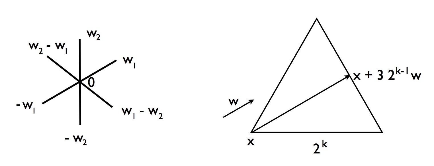
Figure 20. $\Omega$ and a line through a vertex $x$ in the direction $w$ meeting the opposite edge at $3\,2^{k-1}w$.

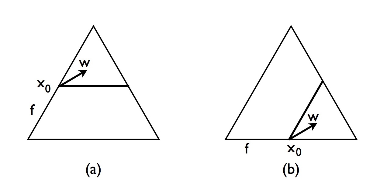
Figure 21. Showing $x_{0}$ as a midpoint of an edge $f$ of a triangle of level $2^{k+1}$ and the direction of $w$ from it.

We claim that under the condition generic-w we have $Q=\bigcup_{k=1}^{\infty}V_{k}$. The only way that $x\in Q$ can fail to be in some $V_{k}$ is that $x\in U_{k}$ for all $k$. Then $x$ is on w-lines through vertices of arbitrarily high level triangles. At least one $w\in\Omega$ occurs infinitely often in this. Fix such a $w$. The vertex of a level $k$ triangle is always the vertex of $6$ such triangles around that vertex. So whenever the w-line passes through a vertex of a level $k$ triangle it also passes into the interior of one of the level $k$ triangles of which this is a vertex and then through the centroid of this level $k$ triangle. Thus the w-line $x+\mathbb{Z}w$ has centroids of arbitrary level on it, violating generic-w.

Let $x=q_{1}+\cdots q_{k}+2^{k}u+3nw=x_{0}+3nw\in V_{k}$ for some $k$, where $n$ satisfies our conventions noted above on the values it may take. Then by the definition of $V_{k}$, $x_{0}$ is not the vertex of any edge of a triangle $T$ of side length $2^{k+1}$ and so $x_{0}$ is the mid-point of an edge $f$ of such a $T$. In particular $x_{0}\notin V_{k}$. Fig. 20 and Fig. 21 indicate, up to orientation, what all this looks like. The edge $f$ is on the highest level line through $x_{0}$ and so determines the stripe of the hexagon at $x_{0}$ and, more importantly, the coloring of the w-line that we are studying. The coloring at $x_{0}$ in the direction $w$ starts red in the case of Fig. 21(a) and blue in the case of Fig. 21(b). The color then alternates along the line in the manner illustrated in Fig. 13.

The color pattern determined here repeats modulo $2^{k+1}Q$ (not $2^{k}Q$), so $V_{k}$ splits into subsets, each of which is a union of cosets of $2^{k+1}Q$ in $Q$,

$$V_{k}=V_{k}^{r}\cup V_{k}^{b}=\bigcup_{w\in\Omega}\bigcup_{n=0}^{2^{k}-1}V^{r}_{k}(w,n)\cup V^{b}_{k}(w,n)\,,$$

corresponding to the red-blue configurations and corresponding also to which $w\in\Omega$ is involved. Here $V^{r}_{k}(w,n)$ is the set of points $q_{1}+\cdots q_{k}+2^{k}u+3nw\in V_{k}$ which start in the direction $w$ with the color red, where $0\leq n<2^{k-1}$ with the boundary conditions on $n$ established as above. The situation with $V^{b}_{k}(w,n)$ is the same except red is replaced by blue. Notice that each $V^{r}_{k}(w,n)$(or $V^{b}_{k}(w,n)$) is a union of $2^{k+1}Q$-cosets for various values of $k$.

Now we need to look at the other aspect to determining the white and gray tiles, namely edge shifting. For this we assume the condition generic-a. Every $x\in Q$ lies on an edge of level $k$ for some $k$. Recall that this means that $x$ is on the edge of a triangle of level $k$ but not one of level $k+1$. The condition generic-a says that such an edge must exist for $x$. Such an edge must then appear as the inner edge $e$ of a corner triangle of a triangle $T$ of level $k+1$. The edge $e$ then shifts towards the centroid of $T$, say in the direction $w\in\Omega$, carrying corresponding diameters in along with it.

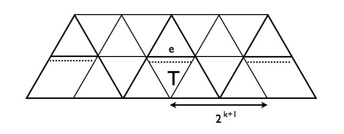
Figure 22. Showing a level $k$ edge inside a triangle $T$ of level $k+1$ and its corresponding shift (dotted line). Note how edge shifting for edges of level $k$ repeats modulo $2^{k+1}$.

Let

$$L_{l}(w):=\{x\in Q\,:\,x\,\mbox{lies on an edge of level $l$ which shifts in the direction $w$ }\}\,.$$

Then $Q=\bigcup_{l=1}^{\infty}\bigcup_{w\in\Omega}L_{l}(w)$. As one sees from Fig. 22, $L_{l}(w)$ is a union of $2^{l+1}Q$-cosets (but not $2^{l}Q$-cosets).

We now put these two types of information together. We display the results in the form of two tables: any $x\in Q$ satisfies

(8) $$x\in V_{k}^{c}(w,n)\cap L_{l}(w^{\prime})$$

for some $c\in\{r,b\}$, $k,l\geq 1$, $w\in\Omega$, $w^{\prime}\in\Omega$.

Notice that $V_{k}^{c}(w,n)\cap L_{l}(w^{\prime})$ is a union of $2^{m}Q$-cosets for $m=\max\{k+1,l+1\}$. So we finally obtain that each of $Q^{wh}$ and $Q^{gr}$ is the union of such cosets. This is what we wanted to show and concludes the proof of the theorem.

7.3. Parity in terms of model sets: the non-generic case

For non-generic sets there are two situations to consider. First of all, let us consider tilings of the minimal hull. Any such tiling $\Lambda^{\prime}$ can be viewed as the limit of translates of a generic tiling, $\Lambda$. Let $\xi(\Lambda)={\bf q}$ and let $W^{wh}$ and $W^{gr}$ denote the two closed windows that define the parity point sets of the tile centers of $\Lambda$. Translation of $t+\Lambda$, $t\in Q$, amounts to translation by $t^{\star}$ of $W^{wh}$ and $W^{gr}$. This is in fact just translation by $t$ but with $t$ seen as an element of $\overline{Q}$. Translation does not affect the type of the tiling (iw-L, iCa-L, etc.).

Convergence of a sequence of translates $t_{1}+\Lambda,t_{1}+t_{2}+\Lambda,\dots$ to $\Lambda^{\prime}$ in the hull topology implies $Q$-adic convergence of $t_{1}+t_{2}+\cdots$, say to ${\bf t}\in\overline{Q}$. The translated sets then also converge to ${\bf t}+W^{c}$, $c=\{wh,gr\}$. However, if ${\bf t}\notin Q$ then we will not necessarily have $\Lambda^{\prime}=\curlywedge({\bf t}+W^{c})$.

Here is what happens. If $u\in\Lambda^{\prime}$ then for large enough $n$, $u\in t_{1}+t_{2}+\dots+t_{n}+\Lambda$ and $u^{\star}\in t_{1}+t_{2}+\dots+t_{n}+W^{c}$. Thus $u^{\star}\in{\bf t}+W^{c}$ and we have that $\Lambda^{\prime}\subset\curlywedge({\bf t}+W^{c})$. On the other hand we have $\Lambda^{\prime}\supset\curlywedge({\bf t}+(W^{c})^{\circ})$. For suppose that $x\in\curlywedge({\bf t}+(W^{c})^{\circ}))$. Then $x^{*}\in({\bf t}+(W^{c})^{\circ})\cap Q^{*}$ and using the convergence $t_{1}+t_{2}+\dots\to{\bf t}$ we see that for large $n$, $x^{*}\in(t_{1}+t_{2}+\dots+t_{n}+(W^{c})^{\circ}))\cap Q^{*}$. Thus for large $n$, $x\in\curlywedge(t_{1}+t_{2}+\dots+t_{n}+W^{c})=t_{1}+t_{2}+\dots+t_{n}+\Lambda$, and so $x\in\Lambda^{\prime}$. We conclude that $\Lambda^{\prime}=\curlywedge(Z)$ for some window $Z$ satisfying ${\bf t}+(W^{c})^{\circ}\subset Z\subset{\bf t}+W^{c}$. This shows that $\Lambda^{\prime}$ is a model set since $Z$ lies between its interior and the (compact) closure of its interior. Also $\partial Z\subset\partial({\bf t}+W^{c})$ has Haar measure $0$ as it was explained in the beginning of Section 7.2.

The remaining cases are the SiCw-L tilings. Let $\Lambda$ be such a tiling, which we may assume to be associated with $\xi(\Lambda)=0\in Q$. Comparing the SiCw-L tiling $\Lambda$ with an iCw-L tiling $\Gamma$ for which $\xi(\Gamma)=0$, we notice that the only difference between $\Lambda$ and $\Gamma$ is on the lines through $0$ in the $w$-directions where $w\in\Omega$. The total index is introduced in [12]. Notice that it is enough to compute that the total index of the set of all points off these $w$-lines is $1$ (see cite[LM1]). Because the set of points off the lines of $w$-directions is the disjoint union of cosets $V_{k}$ (we have seen this earlier), we only need to show that the total index of $\cup_{1}^{\infty}V_{k}$ is $1$, i.e.

$$\sum_{k=1}^{\infty}c(V_{k})=1.$$

Following the construction of $V_{k}$, $k\geq 1$, already discussed above, we compute the coset index of $V_{k}$. Within each $V_{k}$ we need to divide the point set $V_{k}$ into two sets. One is the point set whose points are completely within the $(k+1)$-th level triangles and the other is the point set whose points are lying on the lines of the $(k+1)$-th level triangles. We note that

$$c(V_{1}) = \frac{6}{4\cdot 2^{2}}$$

$$c(V_{2}) = \frac{(2^{1}-1)\cdot 2\cdot 3\cdot 2}{4\cdot 2^{2}\cdot 2^{2}}+\frac{6}{4\cdot 2^{2}\cdot 2^{2}}$$

$$c(V_{3}) = \frac{(2^{2}-1)\cdot 2\cdot 3\cdot 2}{4\cdot 2^{2}\cdot 2^{2}\cdot 2^{2}}+\frac{6}{4\cdot 2^{2}\cdot 2^{2}\cdot 2^{2}}$$

$$\vdots$$

$$c(V_{k}) = \frac{(2^{k-1}-1)\cdot 2\cdot 3\cdot 2}{4\cdot(2^{2})^{k}}+\frac{6}{4\cdot(2^{2})^{k}}.$$

So

$$\sum_{k=1}^{\infty}c(V_{k}) = \frac{6}{4}\left(\frac{1}{2^{2}}+\frac{1}{2^{2}\cdot 2^{2}}+\cdots+\frac{1}{(2^{2})^{k}}\cdots\right)+3\left(\frac{2}{(2^{2})^{2}}+\frac{2^{2}}{(2^{2})^{3}}+\cdots+\frac{2^{k-1}}{(2^{2})^{k}}+\cdots\right)$$

$$~{}~{}~{}~{}~{}-3\left(\frac{1}{(2^{2})^{2}}+\frac{1}{(2^{2})^{3}}+\cdots+\frac{1}{(2^{2})^{k}}+\cdots\right)$$

$$= \frac{6}{4}\left(\frac{1/4}{1-1/4}\right)+3\left(\frac{1/8}{1-1/2}\right)-3\left(\frac{1/16}{1-1/4}\right)$$

$$= 1.$$

8. A formula for the parity

In this section we develop formulae for tilings which determine the parity of each tile of a tiling from the coordinates of the center of that tile. We begin with the formula for parity derived in [19] for the CHT tilings centered at $(0,0)$. These correspond to the triangulation for ${\bf q}=0$. The parity formula for a tile is based on the coordinates of the center of the hexagonal tile. Due to the non-uniqueness of the CHT tilings along the $6$-rays at angles $2\pi k/6$ emanating from the origin, the basic formula is valid only off these rays. Later we show how to adapt this formula to arbitrary ${\bf q}$.

The parity of a tile depends on the relationship of its main stripe to the diameter at right-angles to this stripe. In terms of the triangulation, the parity of a tile depends on two things: the way the triangle edge on which the stripe is located is shifted and the order of the two colors of the color line as it passes through the tile: red-blue or blue-red. Changing the shift or the color order changes the parity, changing them both retains the parity. Thus the parity can be expressed as the modulo $2$ sum of two binary, i.e. $\{0,1\}$, variables representing the shift and the color order. Which parity belongs to which type of tile is an arbitrary decision. In our case we shall make it so that the white tile has parity $1$ and the gray tile has parity $0$.

We introduce here a special coordinate system for the plane (which we really only use for elements of $Q$). We take three axes through $(0,0)$, in the directions of $a_{1},a_{2},-(a_{1}+a_{2})$ with these three vectors as unit vectors along each. For convenience we define $a_{3}:=-(a_{1}+a_{2})$. Each $x\in Q$ is given the coordinates $(x_{1},x_{2},x_{3})$ where $x_{1}$ is the $a_{2}$ coordinate where the line parallel to $a_{1}$ through $x$ meets the $a_{2}$-axis. Similarly $x_{2}$ is the $a_{3}$ coordinate where the line parallel to $a_{2}$ through $x$ meets the $a_{3}$-axis, and $x_{3}$ is the $a_{1}$ coordinate where the line parallel to $a_{3}$ through $x$ meets the $a_{1}$-axis. This is shown in Fig. 23. Notice that $x_{1}+x_{2}+x_{3}=0$. We call these coordinates the triple coordinates.

The redundant three label coordinate system that we use has the advantage that one can just cycle around the coordinates to deal with each of the three $w$-directions. Counterclockwise rotation through $2\pi/3$ amounts to replacing $(x_{1},x_{2},x_{3})$ by $(x_{3},x_{1},x_{2})$.

We note that $x\in Q$ if and only if $x_{1},x_{2},x_{3}\in\mathbb{Z}$. Let $\nu:\mathbb{Z}\longrightarrow\mathbb{Z}$ be the $2$-adic valuation defined by $\nu(z)=k$ if $2^{k}||z$, i.e. if $2^{k}$ divides $z$ but $2^{k+1}$ does not divide $z$. We define $\nu(0)=\infty$. Finally we define $D(z)=2^{\nu(z)}$. Note that $D(-z)=D(z)$. When levels appear, they are related to $\log_{2}(D(z)$.

Now for $x\in Q$ we note that, except for $x=0$, exactly two of $D(x_{1}),D(x_{2}),D(x_{3})$ are equal and the remaining one is larger. This is a consequence of $x_{1}+x_{2}+x_{3}=0$.

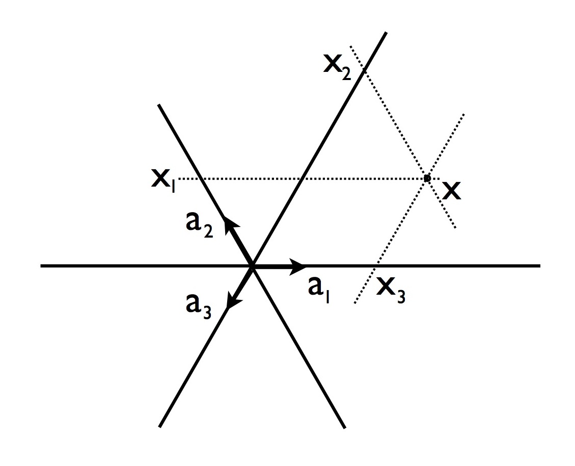
Figure 23. The three coordinate system of labelling points in the plane.

8.1. CHT formula

In this section we derive the formula for parity for the CHT tiling [19]. The CHT tiling has the advantage that all the shifting due to the choice of the triangulation is taken out of the way, and this makes it easier to see what is going on. Our notation and use of coordinates is different from that in [19], but the argument is essentially the same.

Figure 24. Part of the triangulation corresponding to ${\bf q}$ centered at $0$ (indicated by the dot). Triangles of scales $1,2,4$ are shown, as well as part of a triangle of scale $8$.

Fig. 24 shows how the CHT triangulation looks around its center $(0,0)$. The formula for parity is made of two parts each of which corresponds to one the two features which combine to make parity: edge shifting and the color.

First consider the shifting part of the formula. We consider a horizontal line of the CHT triangulation, different from the $a_{1}$-axis. This line meets the $a_{3}$-axis at a point $(n2^{k},-n2^{k},0)$ for some non-negative integer $k$ and some odd integer $n$. This point is the apex of a level $k$ triangle and is the midpoint of an edge from a triangle of level $k+1$ (though the $a_{3}$-axis itself is of infinite level here). As such we see that the horizontal edge to the right from $(n2^{k},-n2^{k},0)$ is shifted downwards. As the edge passes into the next level $k+1$ triangle we see that the shift is upwards. This down-up pattern extends indefinitely both to the right and to the left. In Fig. 25 $n=1$ and $k$ is unspecified, but the underlying idea does not depend on the value of $n$. We now note that the points along the horizontal edge rightwards from $(2^{k},-2^{k},0)$ are $(2^{k},-2^{k}-1,1),(2^{k},-2^{k}-2,2),\dots$, or $x=(2^{k},-2^{k}-x_{3},x_{3})$ in general. Now we note that

(9) $$\left\lfloor\frac{x_{3}}{D(x_{3}+x_{2})}\right\rfloor=\begin{cases}0\quad\mbox{if $x$ corresponds to a shift down edge,}\\ 1\quad\mbox{if $x$ corresponds to a shift up edge\,.}\end{cases}$$

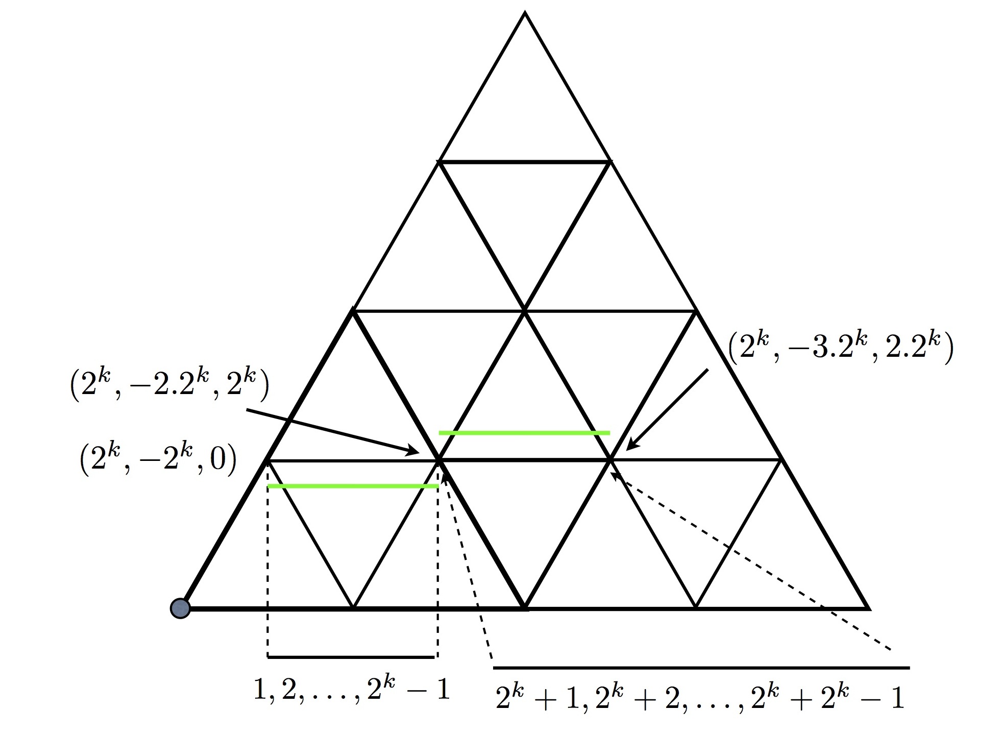
Figure 25. The horizontal line through the point $(2^{k},-2^{k},0)$ is seen as passing through midpoints of consecutive $2^{k+1}$ triangles. The corresponding edges along this line shift downwards and upwards alternately. The points $(2^{k},-2^{k}-m,m)$ with $m=1,2,\dots,2^{k}-1$ are on a shift-down edge. The next set for $m=2^{k}+1,\dots,2^{k}+2^{k}-1$ are on a shift-up edge. The next set, $m=2.2^{k}+1,\dots 2.2^{k}+2^{k}-1$ are on a shift-down edge, etc. The formula $\lfloor\frac{x_{3}}{D(x_{3}+x_{2})}\rfloor=\lfloor m/(2^{k})\rfloor$ accounts for this precisely, varying between $0$ and $1$ according to down and up.

Thus this is the formula for edge downwards ($0$) and edge upwards ($1$). This formula is not valid if $x_{3}\equiv 0\mod 2^{k}$. What distinguishes these bad values is that for these, and these only, $D(x_{2})\neq D(x_{3})$. We see that the fact that we are dealing with a horizontal line (in the direction of the $a_{1}$ axis) is related to the fact that $D(x_{1})$ is the largest of $\{D(x_{1}),D(x_{2}),D(x_{3})\}$, and whenever that condition fails the above formula fails. But then of course we should use the appropriate formula with the indices cycled.

Next we explain the color component of the formula. The underlying idea is much the same, but, as to be expected, the details are a little more complicated. The color lines are the w-lines and are oriented in one of the three $w$ directions. We treat here the case of color lines that are in the vertical direction. The formula utilizes the same three coordinate formulation above. For other w-directions one cycles the three components around appropriately.

Consider the sector of the CHT tiling as indicated in Fig. 26. The figure indicates how the color must be on the $a_{3}$-axis as we proceed in the vertical direction.

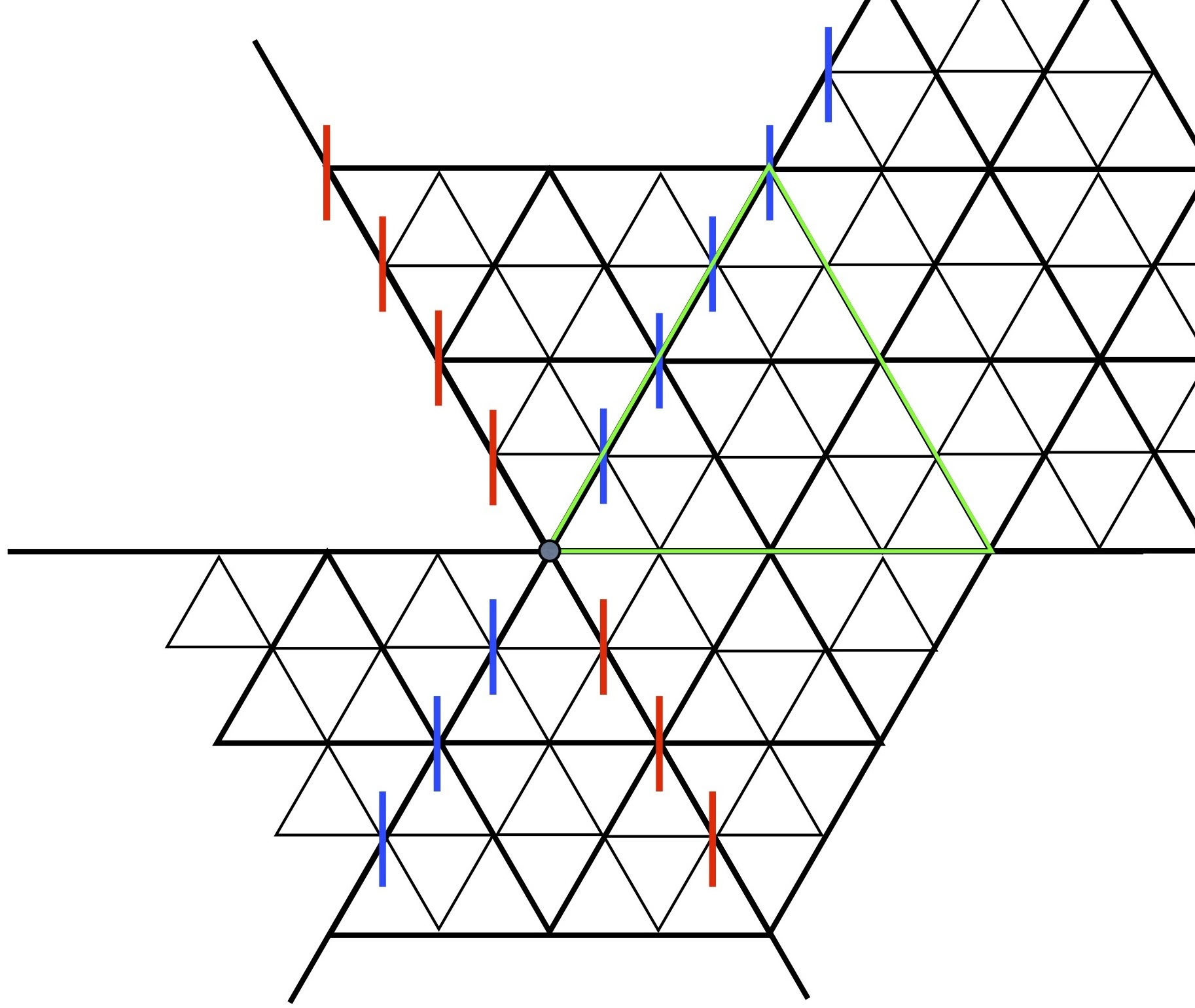
Figure 26. Vertical color lines start with a full blue diameter or full red diameter as shown. The green triangle indicates why the second blue line segment up from the origin is in fact blue. The vertical line is centered at the mid-point of an edge of a level $4$ triangle and passes into one of the level $2$ corner triangles of this level $4$ triangle. The discussion on color shows that it must be blue. All the other blue line segments are explained in the same way. We cannot assign color at the origin itself since the origin is not the mid-point of any edge.

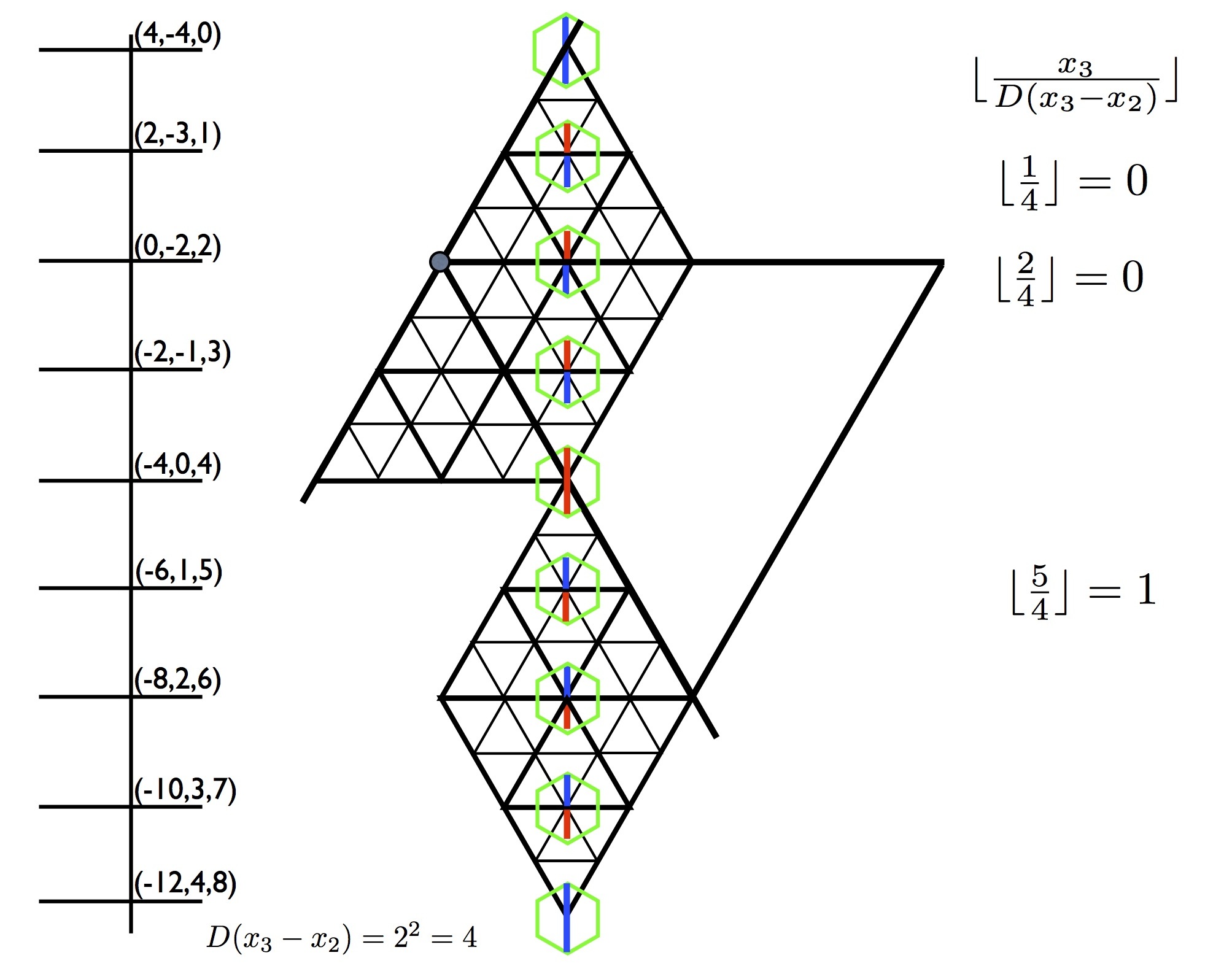
Figure 27. In the figure the small circle indicates $(0,0)$. A vertical color line is shown, which meets the $a_{3}$ axis in the point $p=(4,-4,0)$. The points on this axis are all of the form $(u,-u,0)$, $u\in\mathbb{Z}$. In the CHT tiling set-up, D(u) indicates that the point is a vertex of a level $\log_{2}D(u)$ triangle, in this case $D(4)=4$, so we are on a level $2$ triangle ($2^{2}=4$). We already saw that the color starts with a full blue diagonal at $(4,-4,0)$. Moving down the line to the next point decreases $x_{1}$ by $2$ and increases $x_{2},x_{3}$ by $1$. We note that $x_{3}-x_{2}$ remains constant, and $D(x_{3}-x_{2})=4$. At the second step we cross, at right-angles into another triangle of level $2$, and the color proceeds without interruption. At the $4$th step we are at a vertex that is the midpoint of the side of a triangle of level $3$ and looking up our vertical line we can see that it is passing into a corner triangle of level $4$ – namely where we just came from, and we see a forced full red diagonal. In the first three steps the diameters are all red-blue (top to bottom), whereas after the red-red diagonal the next three steps are blue-red diameters, so the is a switch that affects parity. We can ignore the points with full diameters (they get sorted out in a different w-direction). We note that $\lfloor\frac{x_{3}}{D(x_{3}-x_{2})}\rfloor$ maintains the value $0$ on steps $1,2,3$ and maintains the value $1$ on steps $5,6,7$, showing that the formula notices the change of diameters correctly. If we continue $\lfloor\frac{x_{3}}{D(x_{3}-x_{2})}\rfloor=2$ on the next three step sequence, but modulo $2$ this is the same as $0$.

Most of the explanation for the color part of the formula appears in the caption to Fig. 27. Although that picture seems tied to the point of intersection of the vertical line and the $a_{3}$-axis having the special form $(4,-4,0)$ we note that the same applies whenever $D(x_{3}-x_{2})=4$. It is $D(x_{3}-x_{2})$ that determines the level of the triangle that we are looking at and thus how the stepping sequence will modify the hexagon diameters. In the case where it is $4$ here there are $3$-step sequences of one diagonal type followed by $3$-step sequences of the other type. If $D(x_{3}-x_{2})=2^{k}$ these become $2^{k}-1$ step sequences, and still $\lfloor\frac{x_{3}}{D(x_{3}-x_{2})}\rfloor$ changes by $1$ each time we move from one $2^{k}-1$ step sequence to the next. All sequences start from the full blue diameter with $x_{3}=0$ and $x_{3}$ increases by $1$ at each step.

In putting the two formulas together, we note first of all that although the formulas have been derived along specific $a$ and $w$ axes, the formulas remain unchanged if the same configurations are rotated through an angle of $\pm 2\pi/3$. Likewise the coloring and shifting rules depend on the geometry and not the orientation modulo $\pm 2\pi/3$. The final formula is then effectively just the sum of the two formulas that we have derived, and it is only a question of determining which color of tile belongs to parity $0$.

Theorem 8.1.

[19] In the CHT tilings centered at $(0,0)$, the parity of a hexagonal tile centered on $x=(x_{1},x_{2},x_{3})$ is

$$\mathbb{P}(x)=\left\lfloor\frac{x_{j+2}}{D(x_{j+2}-x_{j+1})}\right\rfloor+\left\lfloor\frac{x_{j+2}}{D(x_{j+2}+x_{j+1})}\right\rfloor\mod 2\,,$$

provided that $D(x_{j})$ is the maximum of $D(x_{j}),D(x_{j+1}),D(x_{j+2})$ and $x_{j+1}\pm x_{j+2}\neq 0$ (subscripts $j$ are taken modulo $3$). ∎

Proof: Referring to Fig. 27, we check the parity of the tile at $(2,-3,1)$. In this case $j$ of the theorem is $1$ and the displayed formula gives the value $0$. On the other hand, the edge shift is down at $(2,-3,1)$ and the shifted edge meets the blue part of the hexagonal diameter, whence the tile is gray. This establishes the parity formula everywhere. ∎

Remark 8.2.

Recall that in the paper we have the convention that white corresponds to $1$ and gray corresponds to $0$.

Remark 8.3.

Notice that in the CHT triangulation centered at $(0,0)$ the hexagon diameters along the three axes defined by $a_{1},a_{2},a_{3}$ have no shift forced upon them and can be shifted independently either way to get legal tilings. These are the hexagons centered on the points excluded by the condition $x_{j+1}+x_{j+2}\neq 0$. Similarly the three w-lines through the origin have no coloring pattern forced upon them and can independently take either. The centers of the hexagons that lie on these lines are excluded by the condition $x_{j+1}-x_{j+2}\neq 0$. In the CHT tiling, the central tile can be taken to be either of the two hexagons and in any of its six orientations. Having chosen one of these $12$ options for the central tile the rest of the missing information for tiles is automatically completed. The parity function $\mathbb{P}$ can be then extended to a function $\mathbb{P}^{e}$ so as to take the appropriate parity values on the $6$ lines that we have just described.

8.2. Parity for other tilings

We can create a formula for arbitrary triangulations $\mathcal{T}({\bf q})$ by the following argument. First of all consider what happens if we shift the center of our triple coordinate system to some new point $c=(c_{1},c_{2},c_{3})_{0}\in Q$ (we are in the triple coordinate system centered at the origin and have indicated this with the subscript $0$). Then relative to the new center $c$, still using axes in the directions $a_{1},a_{2},a_{3}$, the triple coordinates of $x=(x_{1},x_{2},x_{3})_{0}$ are $(y_{1},y_{2},y_{3})_{c}=(x_{1}-c_{1},x_{2}-c_{2},x_{3}-c_{3})$. Thus, if consider ${\bf q}=c$ (or more properly ${\bf q}=(c,c,c,\dots)$) so we are looking at the CHT triangulation now centered at $c$, then the formulae above become

$$\mathbb{P}_{c}(x)=\left\lfloor\frac{x_{j}-c_{j}}{D(x_{j+2}-c_{j+2}-x_{j+1}+c_{j+1})}\right\rfloor+\left\lfloor\frac{x_{j}-c_{j}}{D(x_{j+2}-c_{j+1}+x_{j+1}-c_{j+2})}\right\rfloor\mod 2\,.$$

Consider now an element ${\bf q}=\lim_{k\to\infty}{q_{1}+q_{2}+\dots+q_{k}}$ and the corresponding sequence of triangulations $\{\mathcal{T}(q_{1}+q_{2}+\dots+q_{k})\}$. These converge to $\mathcal{T}({\bf q})$, and with them also we get convergence of edge shifting and color.

It is also true that for any fixed $x=(x_{1},x_{2},x_{3})_{0}$ in the plane the $D$- values of the three triple components of $y=(y_{1},y_{2},y_{3}):=x-(q_{1}+q_{2}+\dots+q_{k})$, as well their various pairwise sums and differences, do not change once $k$ is high enough, since if the $2$-content of a number $n$ is $2^{m}$ then so also is the $2$-content of $n+2^{p}$ for any $p>m$. Thus $\mathbb{P}(x-(q_{1}+q_{2}+\dots+q_{k}))$ is constant once $k$ is large enough, and we can denote this constant value by $\mathbb{P}_{\bf q}(x):=\mathbb{P}(x-{\bf q})$. This defines the parity function $\mathbb{P}_{\bf q}$ for $\mathcal{T}({\bf q})$. Although $\{\mathcal{T}(q_{1}+q_{2}+\dots+q_{k})\}$ is a CHT triangulation, its limit $\mathcal{T}({\bf q})$ need not be. In fact we know that the translation orbit of any of the CHT tilings centered at $(0,0)$ is dense in the minimal hull, and so we can compute a parity function $\mathbb{P}_{\bf q}$ of any tiling of the minimal hull in this way. In the case of generic ${\bf q}$ this results in a complete description of the parity of the tiling. In the case that there is convergence of either a-lines or w-lines (so one is not in a generic case) one can still start with one of the extension functions $\mathbb{P}^{e}$ and arrive at a complete parity description $\mathbb{P}^{e}_{\bf q}$ of any of the possible tilings associated to $\mathcal{T}({\bf q})$.

Corollary 8.4.

The parity function for a generic tiling is $\mathbb{P}_{\bf q}$.

9. The hull of parity tilings

A Taylor–Socolar tiling is a hexagonal tiling with two tiles (if we allow rotations). With the appropriate markings (not the ones we use in this paper), the two tiles can be considered as reflections of each other. If we just consider the tiling as a tiling by two types of hexagons, white and gray, then we get the striking parity tilings, for example, of Fig.  1. We may consider the hull $Y_{Q}$ created by these parity tilings. Evidently $Y_{Q}$ is a factor of $X_{Q}$. In this section we show that in fact the factor mapping is one-to-one – in other words, when we discard all the information of the marked tiles except the colors white and gray – no information is lost, we can recover the fully marked tiles if we know the full parity tiling. The argument uses a tool that is central to the original work of Taylor, but has only played an implicit role in our argument: the Taylor–Socolar tilings have an underlying scaling inflation by a scale factor of $2$. One form of this scaling symmetry is especially obvious from the point of view of the $Q$-adic triangularization.

9.1. Scaling

Suppose that we have a Taylor–Socolar tiling with $\mathcal{T}({\bf q})$, where ${\bf q}=(q_{1},q_{1}+q_{2},$ $\dots,q_{1}+\cdots+q_{k},\dots)$. Then $q_{1}+2Q$ is the set of triangle vertices of all triangles of level at least $1$. To make things quite specific, which we need to do to go on, we choose $q_{1}\in\{0,a_{1},a_{2},a_{1}+a_{2}\}$. In the same way we shall assume $q_{2}\in 2\{0,a_{1},a_{2},a_{1}+a_{2}\}$, and so on. We can view $q_{1}+2Q$ as being a new lattice (even though it may not be centered at $0$) and then we note that ${\bf q}^{\prime}:=(0,q_{2},q_{2}+q_{3},\dots,q_{2}+\cdots+q_{k},\dots)$ is another triangularization (now of this larger scale lattice, and taken relative to an origin located at $q_{1}$) that determines a Taylor–Socolar tiling with hexagonal tiles of twice the size. Each of these new double-sized hexagons is centered on a hexagon of the original tiling which itself is centered at a vertex of a level $1$ triangle.

The new triangularization has its own edge shifting, and since all that has happened is that all the lines of the triangularization that do not pass through a vertex of a level 1 triangle have gone, we can see that the shifting rules mean that the remaining lines still shift exactly as they did before. Also the whole process of coloring the new double-size hexagons goes just as it did before. Fig. 28 shows why the coloring of the new double-size hexagons is the same as the coloring of the original size hexagons on which they are centered.

What happens if the Taylor–Socolar tiling $\mathcal{T}({\bf q})$ is non-generic? A tiling is non-generic if and only if it has an $a$-line or a $w$-line of infinite level. From the definitions, one sees that just rescaling so that the level $0$ triangles vanish and all other triangles are now lowered in level by $1$ still leaves infinite level lines in tact and so we are still in a non-generic case. We can also see this in detail. Non-generic tilings happen if and only if ${\bf q}\in x+\overline{\mathbb{Z}_{2}}\,a$ or ${\bf q}\in x+\overline{\mathbb{Z}_{2}}\,3w$ for some $x\in Q$. Consider ${\bf q}^{\prime}=(0,q_{2},q_{2}+q_{3},\dots,q_{2}+\cdots+q_{k},\dots)\in 2\overline{Q}$. For definiteness, take the second case. Then we can write

$${\bf q^{\prime}}\in-q_{1}+x+\alpha 3w+\overline{\mathbb{Z}_{2}}3(2w)$$

where $\alpha=0$ if $-q_{1}+x\in 2Q$ and $\alpha=1$ if $-q_{1}+x\notin 2Q$. This gives ${\bf q^{\prime}}\in x^{\prime}+\overline{\mathbb{Z}_{2}}3(2w)$ for some $x^{\prime}\in 2Q$, and we are in the non-generic case again. The same thing happens in the other case.

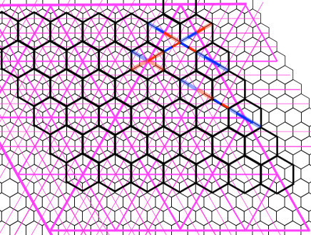
Figure 28. This shows how the scaled up hexagon inherit the colors of the smaller hexagons on which they are centered. The coloring is carried out by the same procedure that was used to color the original sized hexagons, though now the diameter sizes have doubled and only the lines of level at least $1$ are used.

This scaling self-similarity of the Taylor–Socolar tilings is an important part of Taylor’s original construction of the tilings. Here we see self-similarity arise from the simple procedure of ‘left shifting’ the $Q$-adic number ${\bf q}$. Geometrically, shifting means subtracting $q_{1}$ and dividing by $2$. We have restricted $q_{1},q_{2},\dots$ to be specific coset representatives so that this process of subtraction/division is uniquely prescribed.

We can also work this process in the other direction. Given ${\bf q}$ there are four ways in which to choose a coset from $(\frac{1}{2}Q)/Q$ and for each of these choices we get a new element of the $Q$-adic completion of $\frac{1}{2}Q$. Thus reducing the scale by a factor of $2$ we obtain new triangularizations and hexagonal tilings. The original tiling reappears via the scaling up by a factor of $2$, as we have just seen. Also note that the new tilings are non-generic if and only if the original tiling was since infinite $a$ or $w$ lines remain as such in the new tilings. Thus we see that scaling has no effect on the generic or non-generic nature of the tilings in question. It is also clear that CHT tilings, iCw-L tilings, and even SiCw-L tilings all transform into tilings of the same type.

9.2. From parity to Taylor–Socolar tilings

Creating a full Taylor–Socolar tiling from a parity tiling is carried out in two steps: first work out the triangularization, then add the color. For generic tilings the second step is superfluous. Even for non-generic tilings, the fact that the tiling is non-generic is an observable property of the triangularization and then knowing the parity makes it straightforward to recover the colouring along the ambiguous line or lines. The color is not a significant issue and we discuss only the recovery of the triangularization here.

So let us assume that we have a parity tiling $\mathcal{T}_{P}$ that arises from some tiling $\mathcal{T}({\bf q})$ which at this point we do not know. To obtain the triangularization, i.e. ${\bf q}$, we need to work out the translated lattices $q_{1}+2Q,q_{2}+4Q,\dots$. These are the sets of vertices of the triangles of levels $\geq 1$, $\geq 2$, etc. Suppose that we have a method that can recognize the translated lattice $q_{1}+2Q$ (which is a subset of the hexagon centers of the parity tiling). Then, in effect, we know $q_{1}$ (at least modulo $2Q$, which is all we need to know about it). We can now imagine changing our view point to double the scale by redrawing the parity tiling with double sized hexagonal tiles at the points of $q_{1}+2Q$ and while retaining the color. We know that this new tiling will be the parity tiling of the scaled up tiling $q_{1}+\mathcal{T}({\bf q^{\prime}})$ where ${\bf q}^{\prime}=(0,q_{2},q_{2}+q_{3},\dots,q_{2}+\cdots+q_{k},\dots)$.

At this point we can proceed by induction to determine $q_{2}+4Q$, rescale again and get $q_{3}+8Q$, and so on. So what is needed is only to determine the vertices of the level $\geq 1$ triangles, or equivalently determine which hexagons of the parity tiling lie on such vertices.

Let us call a patch of $7$ tiles which consists of a tile in the center and its $6$ surrounding tiles a basic patch of $7$ tiles. The key observation is that in a Taylor–Socolar-tiling it never happens that a basic patch of $7$ tiles whose center tile is a corner tile of a triangle of level $\geq 1$ has $5$ surrounding tiles all of the same color. Thus in the parity tiling the hexagons centered on the (as yet unknown) vertices of the level $\geq 1$ triangles, cannot appear as shown in Fig. 29 or in any of their rotated forms. On the other hand, as we shall see, for all the other cosets of $Q$ modulo $2Q$ there are points around which such patches (up to rotational symmetry) do occur. Furthermore we do not have to look far in any part of the tiling to find such examples. This is the feature that allows us to distinguish the coset $q_{1}+2Q$ from the remaining cosets of $Q\mod 2Q$.

The actual proof goes in three steps. In the first we show the ‘no five hexagons’ rule for hexagons centered on the vertices of triangles of level $1$. Next we do the same for all the vertices of triangles of level $\geq 2$. This deals with all hexagons centered on $q_{1}+2Q$. Finally we show that for each of the other cosets of $Q\mod 2Q$ the ‘no five hexagons’ rule fails at least somewhere.

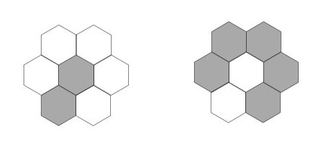
Figure 29. Patches of (parity) tiles in which the central tile has $5$ of its surrounding tiles of the same color.

1. The vertices of $1$-level triangles: We wish to show that around each hexagon centered on a point of $q_{1}+2Q$ there are at least two different pairs of tiles of with mis-matched colors amongst its six surrounding tiles (and hence the no five-hexagons rule is true). This is explained in the text below and in Fig. 30.

   

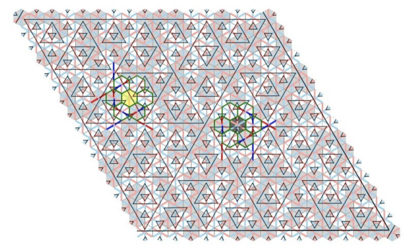
   Figure 30. Examples are shown which demonstrate how we can see that around each hexagon centered on a level $1$ vertex of $q_{1}+2Q$ there are at least two different pairs of tiles with mis-matched colors amongst its six surrounding tiles. The two cases correspond to a level $1$ vertex at the mid-point of a level $2$ triangle and a level $1$ vertex a non-midpoint of a higher level triangle. As explained in the text, one pair is found in a uniform way in both cases. The other pair is found by one method in the first case and another method in the other.

   There are two different situations for a hexagon $H$ centered on the vertex $v$ of a $1$-level triangle. One is the case that $v$ is at the midpoint of a $2$-level triangle. This is indicated on the left side of Fig. 30. The other is the case that $v$ is on the edge of a $n$-level triangle where $n\geq 3$. This is indicated on the right side of Fig. 30. In both cases, we note that the two tiles on opposite sides of $H$ which share the long edge of a triangle of level $\geq 2$ have different colors. The reason is the following. Apart from the red-blue diameters, the long red and blue diameters and black stripes are same for the both the Taylor–Socolar tile and the reflected Taylor–Socolar tile. However the red and blue diameters of the middle tiles of $2$-level triangles determine different red-blue diameters for the two tiles, and so they have different parity.

   Now we wish to find another pair of tiles with opposite colors for each of the cases. Let us look at the first case (see the left side of Fig. 30). Consider the corner of the level $3$ triangle $T$ that is defined by $H$, and consider the two edges of $T$ that bound this corner. The red and blue diameters of the tiles at the mid-points of these two edges of $T$ determine different red-blue diameters for two neighbouring tiles in the surrounding tiles of $H$. This again results in different parities.

   Finally consider the second case (see the right side of Fig. 30). Notice that the long black stripe of $H$ is the part of the long edge of $3$ or higher level triangle. If this long edge is from a level $4$ or higher triangle, we consider just the part of it that is the level $3$ triangle $T$ whose edge coincides with the stripe of $H$. The red and blue diameters of the tile centered on the mid-point of this edge of $T$ determine different red-blue diameters for two of the ring of tiles around $H$, as shown.

2. The vertices of level $\geq 2$ triangles: Next we look at the six tiles surrounding the corner tiles of level $\geq 2$ triangles in a Taylor–Socolar tiling. Notice that the pattern of the colored diameters of six surrounding tiles is same for every corner tile of a level $2$ or higher triangle, Fig. 31.

   

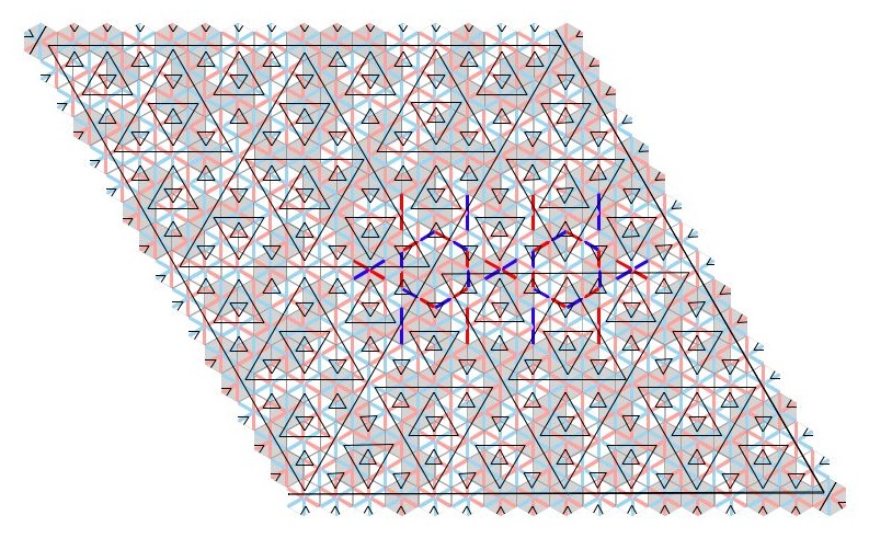
   Figure 31.

   So what determines the basic patches of $7$ tiles around the corner tiles of level $2$ or higher triangles is the pattern of black stripes on it. Furthermore, there is a one-to-one correspondence between these basic patches of $7$ tiles and the basic patches of $7$ tiles of white and gray colors. This is shown in Fig. 32. The key point is that this means that the basic patches of $7$ tiles around the vertices of the level $2$ or higher triangles already determine the coloring.

   

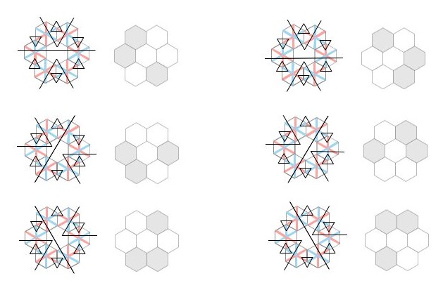
   Figure 32. The edge and color patterns and corresponding parity patterns that can occur in the hexagons surrounding the corners of triangles of level $\geq 2$.

   At this point we know that all the vertices of level $\geq 1$ have at least two tiles of each color in the ring of any basic patch of 7 tiles.

3. Seeing how the other cosets of $Q$ mod $2Q$ violate the ‘two tiles of each color in the ring of any basic patch of $7$ tiles’ rule. From a given parity tiling, there are four choices in determining the $1$-level triangles. One of these is the coset $q_{1}+2Q$, and we know that the $7$ tile patches around each of these points satisfy the ‘no five-hexagon’ rule. However the three choices, corresponding to the other three cosets of $Q\mod 2Q$ all have some $7$ tile patches that violate the rule. We can see violations to the rule for each of the other three cosets in Fig. 33, which is a small piece from the lower right corner of Fig. 1. Since any parity tilings in the hull are repetitive, we observe the patches frequently over the parity tiling. Furthermore, since there is only one way which is allowed to determine $1$-level triangles, it does not depend on where one starts to find the $1$-level triangles. They will all match in the end.

   

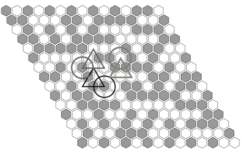
   Figure 33. Here we see three violations to the five-hexagons rule, the rings of hexagons being indicated by the circles. The shaded triangles show how the cosets determined by the center look, and show that the violating hexagons are from three different cosets. The hexagonal pattern comes from the lower right corner of Fig. 1.

This finishes the discussion of how the coset $q_{1}+2Q$ is identified in the parity tiling $\mathcal{T}_{P}$. The scaling argument shows that we can continue the process to identify $q_{2}+4Q,q_{3}+8Q$ and so on. This finally identifies $\bf q$. In fact, even stronger, once we identify $q_{2}+4Q$, we can use the one-to-one correspondence between these basic patches of $7$ tiles and the basic patches of $7$ tiles of white and gray colors as it is shown in Fig. 32 to determine the entire triangularization.

We note two things here: that this argument of this subsection has not required that the tiling be generic, and that the process of reconstruction of the triangularization from a parity tiling is local in character.

We conclude that the parity hull loses no color information, and hence the factor mapping from the Taylor–Socolar hull to the parity hull that simply forgets all information about each tile except for its parity, is in fact an isomorphism. In fact the two hulls are mutually locally derivable (MLD) in the sense that each tiling in one is derivable from a corresponding tiling in the other, using only local information around each tile (see [9]).

Corollary 9.1.

Each Taylor–Socolar tiling and its corresponding parity tiling are mutually locally derivable. ∎

10. Concluding remarks

The paper has developed an algebraic setting for the Taylor–Socolar hexagonal tilings. This approach leads naturally to a cut and project scheme with a compact $Q$-adic internal space $\overline{Q}$. We have determined the structure of the tiling hull and in particular the way in which it lies over compact group $Q$. Each tiling is a model set from this cut and project formalism. The corresponding parity tilings are in fact completely equivalent to the fully decorated tilings. We have also reproved the parity formula of [19].

The tiling is both remarkably simple and remarkably subtle. The parity tilings remain fascinating and inviting of further study.

11. Acknowledgment

We are grateful to Michael Baake and Franz Gähler for their interest and helpful suggestions in the writing of this paper, and to Joan Taylor who provided the idea behind §9.

References

- [1]
- [2] S. Akiyama and J.-Y. Lee, The computation of overlap coincidence in Taylor–Socolar substitution tilings, Preprint (2012).
- [3] M. Baake and F. Gähler, Oral communications.
-
[4]
M. Baake and U. Grimm, A hexagonal monotile for the Euclidean plane,
talk at the KIAS Workshop on The Mathematics of Aperiodic Order (2010).
http://vod.mathnet.or.kr/sub1.php?key_s_titleTheMathematicsofAperiodicOrder - [5] M. Baake, D. Lenz, R. V. Moody, Characterizations of model sets by dynamical systems, Ergodic Theory and Dynamical Systems 27 (2007), 341-382.
- [6] M. Baake and R. V. Moody, Weighted Dirac combs with pure point diffraction, J. reine engew. Math. 573 (2004), 61– 94.
- [7] M. Baake, M. Schlottmann, and P. D. Jarvis, Quasiperiodic tilings with tenfold symmetry and equivalence with respect to local derivability, J. Phys. A, 19 (1991), 4637-4654.
-
[8]
D. Frettlöh, Nichtperiodische Pflasterungen mit ganzzahligem Inflationsfaktor,
Ph.D. thesis, Universität Dortmund, 2002,
http://www.math.uni-bielefeld.de/baake/frettloe/papers/diss.pdf -
[9]
D. Frettlöh and E. Harriss, Tilings Encyclopedia
http://tilings.math.uni-bielefeld.de/ - [10] F. Gähler, A. Julien, J. Savinien, Combinatorics and topology of the Robinson tilings, C. R. Acad. Sci. Paris, Ser. I (2012), in press.
- [11] B. Grünbaum and G.C. Shephard, Tilings and Patterns, W.H. Freeman, 1987.
- [12] J.-Y. Lee and R. V. Moody, Lattice substitution systems and model sets, Discrete and Computational Geometry 25 (2001), 173–201.
- [13] J.-Y. Lee, R. V. Moody, and B. Solomyak, Pure Point Dynamical and Diffraction Spectra, Ann. Henri Poincaré 3 (2002), 1003–1018.
- [14] R. V. Moody, Model sets : a survey, in : From quasicrystals to more complex systems, eds. F. Axel and J. -P. Gazeau, Les Editions de Physique, Springer-Verlag, Berlin (2000), 145-166.
- [15] Roger Penrose, Remarks on a tiling: Details of a -aperiodic set, in The mathematics of long-range aperiodic order, ed. R. V. Moody, NATO ASI Series C:489, Kluwer, 1997.
-
[16]
Roger Penrose, Twistor Newsletter, Reprinted in Roger Penrose: Collected Works, Vol.6: 1997-2003, Oxford University Press, 2010. http://people.maths.ox.ac.uk/lmason/Tn/,
see specifically: http://people.maths.ox.ac.uk/lmason/Tn/41/TN41-08.pdf,
http://people.maths.ox.ac.uk/lmason/Tn/42/TN42-09.pdf,
http://people.maths.ox.ac.uk/lmason/Tn/43/TN43-11.pdf, (1996, 1997). - [17] R. M. Robinson, Undecidability and nonperiodicity for tilings of the plane, Invent. Math. 12 (1971), 177–209.
- [18] M. Schlottmann, Generalized model sets and dynamical systems, in: Directions in mathematical quasicrystals, M. Baake and R. V. Moody, eds., CRM Monograph Ser. 13, AMS, Providence, RI(2000), 143-159.
- [19] J. Socolar and J. Taylor, An aperiodic hexagonal tile, Journal of Combinatorial Theory, Series A 118 (2011), 2207–2231.
-
[20]
J. Taylor, Aperiodicity of a functional monotile,
Preprint (2010),
http://www.math.uni-bielefeld.de/sfb701/files/preprints/sfb10015.pdf